Intelligent Flight Procedure Design: A Reinforcement Learning Approach with Pareto-Based Multi-Objective Optimization

Abstract

Current flight procedure design primarily relies on expert experience, lacking a systematic approach to comprehensively balance safety, route simplification, and environmental impact. To address this challenge, this paper proposes a reinforcement-learning-based method that leverages carefully crafted reward engineering to achieve an optimized flight procedure design, effectively considering safety, route simplicity, and environmental friendliness. To further enhance performance by tackling the low sampling efficiency in the replay buffer, we introduce a multi-objective sampling strategy based on the Pareto frontier, integrated with the soft actor–critic (SAC) algorithm. Experimental results demonstrate that the proposed method generates executable flight procedures in the BlueSky open-source flight simulator, successfully balancing these three conflicting objectives, while achieving a 28.6% increase in convergence speed and a 4% improvement in comprehensive performance across safety, route simplification, and environmental impact compared to the baseline algorithm. This study offers an efficient and validated solution for the intelligent design of flight procedures.

1. Introduction

Flight procedures are defined as the systematic operational steps established for aircraft, outlining the routes, altitudes, and speeds from takeoff to landing. These procedures are a critical component in ensuring flight safety, optimizing operational efficiency, and mitigating environmental impacts. Based on the navigation methods employed, flight procedures are generally classified into two main categories: performance-based navigation (PBN) procedures and conventional navigation procedures. Conventional navigation procedures rely on terrestrial navigation aids, such as very-high-frequency omnidirectional range/distance measuring equipment (VOR/DME). The design of flight routes under these procedures is constrained by the geographical coverage of ground-based stations, which limits flexibility and presents challenges in meeting the demands of complex airspace environments. In contrast, PBN procedures leverage the integration of global navigation satellite systems (GNSS) and onboard navigation technologies to enable precise alignment with aircraft performance capabilities. This allows for the design of more accurate and adaptable flight paths [1,2], offering significant benefits in terms of route simplification and noise pollution reduction [3]. As a result, PBN has become the dominant standard in modern flight procedure design, as endorsed and promoted by the International Civil Aviation Organization (ICAO) [4].

In the design of performance-based navigation (PBN) flight procedures, safety is the primary objective. To meet this requirement, flight procedures must be constructed to effectively avoid terrain obstacles, airspace conflicts, and adverse meteorological conditions. Safe aircraft operations are ensured through the delineation of protection areas and the application of minimum obstacle clearance (MOC) standards [5]. From an economic perspective, the focus shifts to optimizing route length, minimizing unnecessary turns, and strategically planning climb gradients to reduce fuel consumption and operational costs [6,7]. Additionally, environmental sustainability has emerged as a critical supplementary principle in contemporary flight procedure design [8]. This principle emphasizes the mitigation of aircraft noise in residential areas by avoiding noise-sensitive zones and implementing low-noise approach trajectories.

Nevertheless, current methodologies for flight procedure design predominantly rely on manual processes. Designers typically employ tools such as computer-aided design (CAD) in conjunction with established standards, such as ICAO Doc 8168 (PANS-OPS), and leverage engineering expertise. Although this approach ensures adherence to safety regulations, it often falls short in adequately addressing operational efficiency and environmental sustainability considerations [9].

In recent years, researchers have increasingly explored the integration of intelligent optimization algorithms into flight procedure design. However, these methods remain constrained by significant limitations. For instance, methods based on reinforcement learning (RL) explore feasible flight paths by interacting with a simulated environment [10,11]. Nonetheless, most studies focus on a single objective, such as minimizing path length or energy consumption, without integrating safety, convenience, and environmental considerations into a unified reward framework, which undermines their ability to manage the trade-offs inherent in multi-objective optimization. Moreover, existing RL approaches lack refined designs for critical factors such as noise impact modeling and dynamic adjustment of protection areas, which restrict their practical applicability in real-world flight procedures [12]. On the other hand, multi-objective optimization algorithms, such as genetic algorithms, can generate Pareto front solutions but rely on offline computations and fixed weight assignments [13]. These methods struggle to adapt to dynamic environments and real-time decision-making requirements. Additionally, they perform poorly when handling complex constraints, such as obstacle avoidance and noise control [14]. Taken together, these limitations highlight the pressing need for a more systematic, adaptable, and constraint-aware optimization framework capable of addressing the multifaceted requirements of modern flight procedure design [15].

The application of intelligent algorithms in aviation optimization has attracted substantial scholarly interest in recent years. Nevertheless, a significant research gap remains in effectively balancing multiple objectives within flight procedure design. Gardi et al. highlighted the potential of Pareto optimization methods to improve safety, efficiency, and environmental performance in flight trajectory design [16]. By leveraging multi-objective optimization algorithms, this approach reduces fuel consumption while simultaneously enhancing flight efficiency. However, it relies on predefined weight assignments and a static optimization framework, which lacks adaptability to dynamic operational environments. As a result, it cannot adjust design parameters in real time to address complex constraints, such as unexpected obstacles or meteorological variations. Furthermore, the lack of explicit integration of environmental objectives—such as noise pollution—into the optimization framework impairs its ability to achieve comprehensive environmental mitigation.

Similarly, Ribeiro et al. (2022) highlight the effectiveness of reinforcement learning (RL) in optimizing airspace structure under complex constraints [17]. Through dynamic adjustments to airspace configurations, this method significantly enhances airspace utilization and operational efficiency. However, the research is limited to structural adjustments and does not address the inherent multi-objective trade-offs in flight procedure design, especially the simultaneous optimization of safety (e.g., obstacle avoidance), operational efficiency (e.g., fuel consumption), and environmental sustainability (e.g., noise reduction). Furthermore, the reward function design in this study is relatively simplistic, inadequately capturing the conflicts and synergies among multiple objectives, which limits its practical applicability in flight procedure design.

To address the aforementioned challenges, this study proposes a reinforcement learning algorithm that incorporates safety, operational efficiency, and environmental sustainability into a weighted reward function. A dynamic weight allocation mechanism is further introduced to facilitate multi-objective collaborative optimization. By continuously adjusting the coordinates of the waypoints, the final trajectory design for the entire departure flight procedure is achieved. The main contributions of this paper are as follows:

• A multi-objective sampling strategy based on the Pareto front is proposed to enhance algorithm efficiency. To address the low sampling efficiency associated with offline reinforcement learning algorithms, this study introduces a multi-objective sampling strategy rooted in the Pareto front, which is integrated with the soft actor–critic (SAC) algorithm. Experimental results indicate that this approach improves convergence speed by 28.6% and increases the multi-objective composite score by 4%. By optimizing the exploration and exploitation of the state space, the approach significantly improves algorithm efficiency, thereby meeting the rapid convergence and computational demands of flight procedure design.
• A reinforcement learning environment that integrates safety, simplicity, and environmental sustainability for flight procedure design tasks is developed. Within this framework, this research constructs an environment that comprehensively addresses the multi-objective optimization of safety, simplicity, and environmental sustainability. Through careful reward engineering, a suitable set of reward functions is identified, which effectively balances the trade-offs among these conflicting objectives. These reward functions guide the reinforcement learning algorithm in discovering optimal strategies for complex flight tasks.
• The executability and performance of the flight procedures are validated. The designed flight procedures are executed within the BlueSky open-source simulation platform. Experimental results demonstrate that the flight procedures developed using the proposed method are executable and perform as expected.

2. Related Work

2.1. Flight Procedure Design

Currently, flight procedure design methodologies predominantly rely on expert knowledge and standardized guidelines, including ICAO’s PANS-OPS (Procedures for Air Navigation Services—Operations) and the FAA’s TERPS (Terminal Procedures). These approaches prioritize compliance with safety regulations and are widely used in the development of standard instrument departures (SIDs) and approach procedures. For instance, the guidelines outlined in the relevant document [18] emphasize adherence to ICAO Doc 8168, which is designed to ensure obstacle clearance and flight safety. However, the predominant emphasis on safety in these methodologies often comes at the expense of operational efficiency and environmental sustainability.

As shown in

Table 1. Comparison of different methods.

Method	Current Status	Safety	Convenience (Trajectory Shortening)	Environmental Consideration
CAD Tools (Traditional Design)	Relies on expert experience and standard regulations, widely used	Emphasizes safety compliance, lacks dynamic adaptability	Fixed routing, possible extended trajectory	Noise and emissions not fully considered
Heuristic Approach	Balances fuel and time, highly computational, already in use	Safety is treated as a constraint, not directly optimized	Subjective weight assignment, affects efficiency	Noise and fuel optimization, complex trade-off
Reinforcement Learning (RL)	Emerging technology, dynamic strategy adjustment, limited application	Training instability, no guaranteed safety	Potential for shortened trajectory, high data requirement	Theoretically can optimize noise and emissions

, different methods for flight procedure design have their own advantages and limitations in terms of safety, convenience, and environmental considerations. Research has revealed substantial limitations in traditional methods, particularly in their ability to balance safety, convenience, and environmental factors. While safety remains the primary objective, this emphasis often leads to overly complex procedures that increase the workload for both pilots and air traffic controllers, thus reducing convenience. Furthermore, environmental concerns, such as fuel consumption and noise reduction, are often neglected. For instance, relevant studies [19] emphasize the importance of noise abatement procedures during the design process. However, in practice, environmental objectives are often subordinated to operational efficiency. Moreover, a study by E. Israel et al. [20] highlights that although environmental impacts can be assessed, existing methodologies lack a systematic framework capable of simultaneously optimizing all objectives.

Global aviation modernization initiatives, such as the United States’ NextGen and Europe’s SESAR, stress the importance of efficiency and environmental sustainability. However, existing research [21] indicates that progress in incorporating environmental considerations within flight procedure design remains limited. In particular, achieving an effective trade-off among safety, operational efficiency, and environmental sustainability within a unified multi-objective optimization framework continues to pose a substantial challenge. Consequently, there is a pressing need to develop more intelligent and adaptive methodologies capable of addressing the multi-faceted demands of modern flight procedure design.

2.2. Sampling Strategies in Reinforcement Learning

The sampling strategy in reinforcement learning significantly influences the learning efficiency and performance of algorithms. Traditional uniform sampling strategies, while simple and unbiased, have notable limitations. They fail to distinguish the importance of individual experiences, often overlooking critical turning points, which reduces sample utilization [22]. Additionally, in sparse reward scenarios, uniform sampling necessitates extensive data to cover essential areas, leading to slow convergence [23].

To address these challenges, a range of enhanced sampling strategies have been proposed. Notably, prioritized experience replay (PER) has gained attention for its effectiveness [22]. PER employs a priority mechanism based on temporal-difference (TD) error, enhancing the efficiency of critical experience utilization and thereby accelerating convergence. The priority of each experience is defined as illustrated in Equation (1):

$$p_i=\left|{\delta }_i\right|+ϵ$$

(1)

where ${\delta }_i$ is the TD error and $ϵ$ is a small constant to prevent zero sampling probability. Research indicates that PER can enhance sample efficiency by a factor of 3 to 5 [22]. However, PER introduces bias due to non-uniform sampling, which alters the distribution of gradient updates. To mitigate this, importance sampling (IS) weights are used for bias correction, as illustrated in Equation (2):

$${\omega }_i={(N·p_i)}^{-\beta }$$

(2)

where $\beta$ controls the correction strength. With an appropriate decay of $\beta$, PER can converge to the same optimal policy as uniform sampling [24].

In addition to PER, other sampling strategies have been developed. Model-based priority methods utilize a dynamics model to predict future state values. However, their effectiveness is contingent on the accuracy of the model [25]. Hierarchical importance sampling segments experiences by time or features but often relies on prior knowledge, which limits its adaptability [26]. Exploration-driven sampling prioritizes samples from underexplored states, enhancing exploration efficiency, but it necessitates a delicate balance to prevent policy instability [27].

In summary, while uniform sampling is simple to implement, it suffers from low efficiency and slow convergence [22]. PER improves sampling efficiency but introduces bias and complexity [22,24]. Future research may focus on adaptive priority mechanisms, distributed priority architectures [28], and deeper theoretical analyses of PER, aiming to enhance the performance and practicality of reinforcement learning algorithms.

3. Methodology

3.1. Problem Formulation

In this work, models are developed to optimize aircraft departure procedures by focusing on safety through protection zones and obstacle clearance, simplicity via turn angles and path length, and environmental impact with regard to noise pollution.

3.1.1. Safety

Safety serves as the primary objective in the optimization process and is evaluated based on the delineation of protection zones for each segment between consecutive waypoints. The design of these protected areas must adhere to the requirements for straight-out departures, ensuring that aircraft can avoid ground obstacles during the takeoff phase, thereby safeguarding flight safety [29].

The departure protection area is divided into a primary zone and a secondary zone, as illustrated in Figure 1. The primary zone is the area directly above the aircraft’s departure trajectory, while the secondary zone extends to the sides of the primary zone, with dimensions equal to those of the primary zone. This study evaluates the safety of different departure segments by analyzing obstacle data within the protected zones. When obstacles are present within these areas, the aircraft may be required to modify its climb gradient to avoid them. Particular attention is given to the impact of obstacle identification surfaces (OIS), which serve as a critical reference for identifying route obstacles [30].

In accordance with the regulations established by the International Civil Aviation Organization (ICAO), the minimum climb gradient for an aircraft must not be less than 0.033 [31]. When the actual climb gradient of the aircraft exceeds this value, it indicates that the aircraft must undertake a steeper ascent to avoid obstacles, potentially compromising safety. Conversely, if the aircraft maintains a climb gradient of 0.033 within the protected area, with no obstacles in either the primary or secondary zones, it indicates a high level of safety for the departure segment. The obstacle identification surface (OIS) is a distinct sloped area designed for the effective identification and assessment of obstacles within the departure protection area, as illustrated in Figure 2.

Specifically, the safety settings are categorized into three ratings: low, medium, and high. The highest rating indicates that no obstacles are within the protected area of the flight segment, resulting in a high safety level. The medium rating applies when obstacles are present within the protected area; however, due to factors such as the distance and height of the obstacles relative to the flight segment, the OIS surface does not intersect with any obstacles, and the aircraft’s climb gradient remains constant at 0.033. In this case, safety is evaluated based on the projection distance of the obstacles from the flight segment. The lowest safety rating is assigned when obstacles are present within the primary protected area, resulting in an increased climb gradient for the aircraft. In this scenario, the higher the climb gradient, the lower the safety level, indicating that the configuration of the flight segment is unreasonable.

The safety objective function $G_{\mathrm{safe}}$ (3) is defined as follows:

$$G_{\mathrm{safe}}=\left\{\begin{array}{cc}3,\hfill & \mathrm{no}\mathrm{obstacles}\hfill \\ 2,\hfill & \mathrm{obstacles}\mathrm{present},\mathrm{and}\mathrm{the}\mathrm{distance}\mathrm{between}\mathrm{the}\mathrm{aircraft}\mathrm{and}\mathrm{obstacles}\ge d_{\mathrm{threshold}}\hfill \\ 1,\hfill & \mathrm{obstacles}\mathrm{present},\mathrm{and}\mathrm{the}\mathrm{distance}\mathrm{between}\mathrm{the}\mathrm{aircraft}\mathrm{and}\mathrm{obstacles}\le d_{\mathrm{threshold}},\hfill \\ \hfill & \mathrm{climb}\mathrm{gradient}\le 0.033\hfill \\ 0,\hfill & \mathrm{obstacles}\mathrm{present},\mathrm{and}\mathrm{climb}\mathrm{gradient}\ge 0.033\hfill \end{array}\right.$$

(3)

where $d_{\mathrm{threshold}}$ is the threshold value for the distance between obstacles and the flight segment, distinguishing between “far” and “near”.

3.1.2. Simplicity

In the design of aircraft departure procedures, conciseness is crucial for enhancing operational efficiency. By optimizing the process from takeoff to integration into the flight route, the path length can be significantly reduced, effectively decreasing fuel consumption and harmful emissions. During the design phase, careful consideration must be given to the turning angles and the total length of the route to ensure optimal flight paths and time management.

Conciseness is primarily determined by two factors: the total sum of the angles turned throughout the procedure and the overall length of the procedure. A larger total turning angle in the departure procedure not only increases the flight distance but also leads to additional fuel consumption and time delays. The longer the overall length of the procedure, the longer the aircraft remains airborne, resulting in increased fuel consumption and operational costs.

Given the necessity of ensuring safety, a concise departure procedure should minimize unnecessary turns and flight distances. Specifically, when quantifying conciseness, attention should be focused on the total length of the procedure and the variation in turning angles. A longer total length and greater angle variation correspond to lower conciseness. This represents a dynamic range, and during the quantification process, scaling factors and weights for each component should be continuously adjusted through experimentation.

The convenience function, as illustrated in Equation (4), is expressed as follows:

$$G_{\mathrm{convenience}}={\displaystyle \frac{k}{\theta ·L}}$$

(4)

where $\theta$ is the total turning angle, L is the total length of the procedure, and k is a constant. This function effectively reflects the relationship between the turning angle and the length of the procedure, making it applicable for optimizing flight procedures.

3.1.3. Environmental

Environmental sustainability is a critical consideration in air transportation. In this study, it is quantified primarily in terms of its impact on noise pollution. The evaluation of the environmental sustainability of departure procedures is based on the noise impact on surrounding residential areas, which is typically determined by the population density of these areas and the distance from the residential zones to the aircraft flight path.

Higher population density in residential areas correlates with greater noise impact, as more individuals are affected by the noise generated during aircraft takeoff and landing. In the design of departure procedures, avoiding flight paths over densely populated areas is crucial to minimizing noise disturbances for local residents.

The closer the residential area is to the flight path, the greater the impact of noise pollution. Noise generated by aircraft during low-altitude flight directly affects residents on the ground, particularly during the takeoff phase, when noise levels are typically elevated. Therefore, departure procedures should be designed to maintain maximum distance from residential areas to reduce the noise impact on residents.

The noise function, as illustrated in Equation (5), is defined as follows:

$$G_{\mathrm{noise}}=\sum _{i=1}^N\left(\alpha ·p_i·e^{-\beta d_i}\right)$$

(5)

where $p_i$ represents the population density of the i-th residential area (people/km²), and $d_i$ denotes the distance from the i-th residential area to the flight path.

The parameters are defined as follows:

• $d_i$: the horizontal distance (km) from the flight path to the residential area.
• $\alpha$: a coefficient used to control the influence of population density on noise calculations.
• $\beta$: a parameter that determines the rate at which noise decreases with increasing distance from the flight path.
• N: the total number of residential areas affected by the flight path.

3.2. Reinforcement Learning for Flight Procedure Design

In this section, a modeling approach is proposed for the multi-objective flight procedure design problem, considering safety, convenience, and environmental sustainability from the perspective of reinforcement learning. The framework for the reinforcement learning-based flight procedure design is illustrated in Figure 3, and the reinforcement learning algorithm employed in this study is the soft actor–critic (SAC) algorithm.

As illustrated in Figure 3, the entire framework can be divided into two components: training and execution. The training component is responsible for updating the neural network of the reinforcement learning algorithm, while the execution component facilitates interaction with the environment to gather learning samples.

In the training phase, the replay buffer [32] stores experience tuples $(s,a,r,s^{\prime },d)$ collected during the execution phase. In this tuple, s represents the current state information; a denotes the action output by the soft actor–critic (SAC) algorithm; r is the scalar reward calculated by the reward model based on the new state information, which is used to evaluate the quality of the action; $s^{\prime }$ indicates the next state information after executing action a; and d is a termination signal indicating whether the episode has ended. These data support the training of the neural network through random sampling from the replay buffer, facilitating updates to the Q-value estimates of the critic network, optimization of the policy of the actor network, and adjustment of the parameters of the target critic network, thereby enabling continuous learning and improvement of the SAC algorithm.

In the execution phase, the SAC algorithm outputs new waypoint latitude and longitude coordinates based on the state information. The environment computes the new state information of the flight procedure based on the input coordinates, which includes information related to safety, simplicity, and environmental sustainability, such as the relative position of obstacles, procedure gradient, total procedure length, and heading change. The new state information is subsequently processed by the reward model and the SAC algorithm. The reward model outputs a reward value based on the new state information to evaluate the quality of the actions produced by the algorithm, thereby supporting the selection of the next waypoint coordinates in the SAC algorithm.

In this study, a reward engineering approach was employed to determine the reward function. While keeping the hyperparameters of the soft actor–critic (SAC) algorithm unchanged, improvements were made to the reward structure based on safety, economy, simplicity, and noise-related factors to enhance the performance of flight procedure design. Specifically, safety reward design was refined by adjusting the magnitude and feature combinations used for evaluation. The economy reward shifted from a total-distance-based metric to a more direct assessment based on state features. The simplicity reward calculation was enhanced by improving the logic for turning characteristics, more accurately encouraging concise trajectories. The noise reward remained consistent to ensure continued mitigation of noise impact.

3.3. Pareto-Based Multi-Objective Optimization

Pareto optimality, a foundational principle in multi-objective optimization first introduced by economists and mathematicians, describes an ideal state of resource allocation where improving one objective necessarily results in the deterioration of at least one other. Formally, let $\mathbf{v}=(v_1,v_2,\dots ,v_k)$ represent one vector, and $\mathbf{w}=(w_1,w_2,\dots ,w_k)$ represent another. The condition for Pareto optimality is that $\forall i\in \{1,\dots ,k\},v_i\le w_i$ and $\exists j\in \{1,\dots ,k\},v_j<w_j$. The set of Pareto-optimal solutions, P, is defined as the set of solutions that cannot be improved without compromising at least one objective, while the set of solutions that dominate the objective space is referred to as the Pareto front, which delineates the boundary of optimality for multiple objectives.

The evaluation of samples based on the Pareto frontier, dominating solutions, and non-dominated solutions inherently defines distinct characteristics of the samples. Motivated by this, we optimize the sampling strategy in the reinforcement learning algorithm. Compared to the random sampling approach typically employed in reinforcement learning, we propose that differentiating samples and adjusting their sampling frequencies accordingly can enhance the learning process, thereby facilitating more effective updates to the algorithm model.

In the context of flight procedure design, it is essential to simultaneously optimize three competing objectives: safety (obstacle avoidance and climb gradient), simplicity (flight distance and turning angles), and environmental sustainability (noise pollution control). For example, enhancing safety may require increasing flight distance or modifying trajectory complexity, which in turn affects economic efficiency and noise distribution. These objectives exhibit nonlinear conflicts, making it challenging to achieve global optimality using traditional single-objective optimization or fixed-weight methods [33]. Based on Pareto optimality theory, this paper constructs a non-dominated solution set to identify the Pareto front in the objective space, thus enabling the dynamic balancing of trade-offs among multiple objectives without the need for pre-defined weights. This approach provides a rigorous mathematical framework and a sound decision-making basis for the comprehensive optimization of flight procedure design. The Pareto model corresponding to the multi-objective optimization problem in flight procedure design is illustrated in Figure 4.

Enhancements have been made to the buffer of the soft actor–critic (SAC) algorithm by implementing a priority experience replay sampling method based on the Pareto-optimal model [22]. The improved buffer is depicted in Figure 5. All experiences from the Pareto-optimal model for departure procedures are stored in the replay buffer. After data storage, each experience is prioritized based on its state evaluated within the Pareto-optimal model for departure procedures. Subsequently, priority experience replay is employed for sampling based on the established priorities, which is then used for loss calculation, gradient descent updates of the policy network, and policy improvement. This process is iteratively repeated.

This paper introduces a scalar definition of priority, where a higher value indicates a greater priority. Each data sample is initially assigned a priority of 0.01 upon storage in the buffer, ensuring it retains a non-zero probability of being sampled and is not excluded from selection. Moreover, the reward function in this environment is designed using a scalarized multi-objective approach, where higher rewards indicate that the data is closer to the Pareto-optimal frontier of the model. As a result, the priority U is positively correlated with the reward r. The priority U is primarily calculated based on the reward r and the different components of the subsequent state $S^{\prime }$, as outlined by the following weighted sum, Formula (6):

$$U=0.01+0.025r+w_1·\mathrm{noise}+w_2·\mathrm{safety}+w_3·\mathrm{simplicity}$$

(6)

Here, noise represents the noise impact, safety refers to safety performance, and simplicity denotes operational simplicity, with $w_1,w_2,$ and $w_3$ being the corresponding weights for each criterion. These weights are designed to address safety, convenience, and environmental factors differently.

The algorithm of the SAC using the Pareto-based sample method is illustrated in Algorithm 1. The improvement in the proposed algorithm lies in the integration of a Pareto-based priority sampling mechanism, which dynamically adjusts the priority U of experiences in the replay buffer based on a weighted combination of noise, safety, and simplicity scores ($U\leftarrow -0.01+0.025·(w_1·noise+w_2·safety+w_3·simplicity)$), enabling a balanced optimization of multiple objectives tailored to flight procedure design.

Algorithm 1 Improved SAC Algorithm with Pareto-Based Replay Buffer Sampling

1: Initialize: SAC components (Actor, Critic, Target Critic networks, Replay Buffer with priority, entropy parameter $\alpha$) 2: Initialize: Environment, initial state s, weights $w_1,w_2,w_3$ for priority calculation 3: Set maximum episode length $max\_ep\_len$ and maximum training timesteps $max\_training\_timesteps$ 4: $timesteps\leftarrow 0$ 5: while $timesteps<max\_training\_timesteps$ do 6:    Reset environment to get initial state s 7:    $episode\_timesteps\leftarrow 0$ 8:    while $episode\_timesteps<max\_ep\_len$ and episode not done do 9:        Sample action $a\sim \pi \left(s\right)$ using Actor network         {Interaction loop} 10:      Execute action a in environment, receive reward r, next state $s^{\prime }$, and done flag d 11:      Store transition $(s,a,r,s^{\prime },d)$ in Replay Buffer with initial priority $U\leftarrow 0.01$ 12:      Calculate Priority:      {Priority calculation based on Pareto-optimal model} 13:      Compute noise, safety, simplicity scores from $s^{\prime }$ 14:      $U\leftarrow 0.01+0.025r+w_1·\mathrm{noise}+w_2·\mathrm{safety}+w_3·\mathrm{simplicity}$ 15:      Priority Sampling:        {Sample batch using priority experience replay} 16:      Sample batch of transitions $(s,a,r,s^{\prime },d)$ from Replay Buffer based on priority U 17:      Neural Network Parameter Update:                {Update loop} 18:      Compute loss and gradients using sampled batch 19:      Optimize policy and Q-value estimation 20:      $s\leftarrow s^{\prime }$                        {Update current state} 21:      $timesteps\leftarrow timesteps+1$ 22:      $episode\_timesteps\leftarrow episode\_timesteps+1$ 23:    end while 24: end while 25: Output: Trained SAC model

4. Experimental Results

4.1. Experimental Setup

4.1.1. Environment Setting

In this study, a performance-based navigation (PBN) departure procedure for Luzhou Airport was developed to optimize the operational environment. The location, initial heading, and elevation information of Luzhou Airport are provided in

Table 2. Luzhou Airport information.

Airport	Longitude	Latitude	Runway	Heading	Elevation
ZULZ	$105.{46889}^{\circ }$ E	$29.{03056}^{\circ }$ N	07	${75}^{\circ }$	335.6 m

. Obstacle information is presented in

Table A1. Obstacle information.

Obstacle Name	Position	Height (m)
base_station	(29.0342, 105.2909)	361.5
base_station	(29.0323, 105.3057)	401.8
High_voltage_iron_tower	(29.0245, 105.3040)	385.6
base_station	(29.0242, 105.3245)	443.2
base_station	(29.0039, 105.2957)	428.1
base_station	(29.0009, 105.2810)	391.4
Tower	(29.0128, 105.2753)	372.6
base_station	(29.0013, 105.2339)	413.5
mountain	(29.0152, 105.2645)	364.4
mountain	(29.0201, 105.2636)	383.6
pole	(29.0214, 105.2636)	394.7
mountain	(29.0224, 105.2642)	408.9
pole	(29.0227, 105.2650)	412.6
mountain	(29.0236, 105.2656)	423.5
base_station	(29.0249, 105.2713)	467.2
base_station	(29.0251, 105.2722)	474.2
mountain	(29.2315, 105.2755)	686
mountain	(29.1344, 105.2932)	701
mountain	(29.1609, 105.3113)	732
mountain	(29.1748, 105.4132)	768
mountain	(29.2119, 105.4631)	683
mountain	(29.1157, 105.4727)	678
mountain	(29.0936, 105.5725)	695
mountain	(28.4847, 105.4702)	719
mountain	(28.4245, 105.4600)	739
base_station	(28.3944, 105.3948)	826
mountain	(28.4059, 105.3858)	883
mountain	(28.3807, 105.3801)	846
mountain	(28.4230, 105.3507)	829
mountain	(28.3601, 105.3308)	837
mountain	(28.3455, 105.2859)	851
mountain	(28.4930, 105.1815)	648
mountain	(29.2213, 105.2622)	666

, and population density information is shown in

Table A2. Population concentration areas.

Name	Position	Number
yunlongzhen	(29.057965, 105.486752)	1000
deshenzhen	(29.090460, 105.413246)	1000
qifengzhen	(29.131086, 105.521877)	800
zhaoyazhen	(28.989800, 105.577030)	1200
shidongzhen	(28.992571, 105.450110)	2000
shunhexiang	(29.150573, 105.445965)	800
shaungjiazhen	(29.025615, 105.432499)	1000
luxain	(29.150530, 105.359453)	10,000
niutanzhen	(29.081750, 105.338461)	1000
hushizhen	(28.948659, 105.361273)	1000
tianxingzhen	(29.105969, 105.287247)	800
haichaozhen	(28.973991, 105.281161)	500
gufuzhen	(29.140192, 105.228960)	500
huaidezhen	(29.004919, 105.222413)	800
xuanshizhen	(29.004919, 105.222413)	1000
zhaohuazhen	(29.025124, 105.118508)	1000
yinanzhen	(28.914062, 105.143877)	800
pipazhen	(29.098428, 105.071649)	800

.

The procedure update process based on reinforcement learning algorithms is shown in Figure 6. The reinforcement learning training environment is updated when the model outputs an action that alters the current state of the flight procedure. This update process sequentially modifies the following parameters for each flight segment: segment altitude, environmental noise information, segment protection area, segment gradient, and segment heading. Subsequently, a decision is made to determine whether the information for all flight segments has been updated. If incomplete, the process switches to the next flight segment for further updates. Once the information for all flight segments is fully updated, the simplicity, noise level, and total distance of the new procedure are calculated.

As shown in Figure 6, the total horizontal length of the flight segments is computed by updating the coordinates of the start and end points of each segment. The distance is then calculated using the two-point distance formula.

Subsequently, the calculation of flight segment noise information is updated. In this step, N is calculated based on the noise from each group of people and their respective calculations. For each group, the noise is represented as the product of the number of people ($people\_num$) and the distance to the observation point ($dis$). The total noise N is computed as follows (Equations (7) and (8)):

$$\mathrm{noise}={\mathrm{people}}_{\mathrm{num}}\times e^{-\mathrm{dis}}$$

(7)

$$N=\sum _{\mathrm{num}}\mathrm{noise}$$

(8)

The calculation of flight segment protection information is then updated. This step involves calculating the protection width $PW$ based on the navigation performance of the route. The procedure sequence is determined by the SID (standard instrument departure) during the calculation. The method for calculating is $rnp$ multiplied by 1.5, where $rnp$ indicates the required navigation performance, with values such as 0.3, 1.0, etc. The distance is converted to nautical miles (nm) and added to a constant of 3704. The calculation for $PW$ is as follows (Equation (9)):

$$PW=1.5\times rnp\times nmtom+3704$$

(9)

This study also involves calculating and updating the stage height. This process requires the revision of the safety height for each stage based on the preceding stage, followed by the computation of the average height. The stage height determination is contingent upon the presence of obstacles within the primary area. In the absence of obstacles, the stage height is conventionally assumed to be 0.033. The safety height $H_{\mathrm{end}}$ for this stage is calculated as shown in Equation (10):

$$H_{\mathrm{end}}=H_{\mathrm{start}}+\mathrm{dis}\times 0.033$$

(10)

If obstacles are present within the parallel projection of the main protection zone, the first step is to assess whether the obstacle identification surface (OIS) intersects with these obstacles. If the OIS does not intersect with any obstacles, the slope of the flight segment remains at the default value of 0.033, and the safety height at the end of the flight segment is calculated according to Equation (10). Conversely, if the OIS intersects with obstacles, the minimum obstacle clearance (MOC) required above the obstacle is calculated to determine the height necessary to safely clear it. After the obstacle is cleared, the flight segment will ascend to the endpoint at a slope of 0.033. In these cases, the safety height at the end of the flight segment, denoted as $H_{\mathrm{end}}$, is computed as outlined in Equation (11), where $H_o$ represents the height of the obstacle, $D_{\mathrm{oe}}$ denotes the distance from the obstacle to the endpoint of the flight segment, and the MOC calculation is given in Equation (12):

$$H_{\mathrm{end}}=H_0+\mathrm{MOC}+D_{\mathrm{oe}}\times 0.033$$

(11)

$$\mathrm{MOC}=D\times 0.8\%$$

(12)

The gradient is calculated as the difference between $H_{\mathrm{end}}$ and $H_{\mathrm{start}}$ divided by the segment length dis, resulting in the average gradient G.

The flight segment calculation is updated, encompassing not only the aircraft’s trajectory but also the directional changes in its orientation.

When the flight segment information is updated, it necessitates a comprehensive revision of the information, including the trajectory, total errors, and distance updates.

The overall simplicity of the procedure is updated. In this section, the simplicity of the procedure is calculated based on an algorithm related to heading. The initial heading difference $\mathrm{\Delta }{A}_0$ is the heading of the first waypoint to be adjusted minus the turning angle of the starting waypoint. Next, a ratio $r_0$ related to $\mathrm{\Delta }{A}_0$ is calculated based on a threshold of 120 degrees, with special handling for a 0-degree difference (by adding an additional 1 to the ratio), as shown in Equation (13). Then, the heading difference $\mathrm{\Delta }{A}_n$ is calculated for each pair of consecutive waypoints, and a similar procedure is applied to compute the corresponding ratio $r_1$, which is then accumulated, as indicated in Equation (14). Ultimately, the simplicity value is the sum of $r_0$ and the accumulated $r_1$, as expressed in Equation (15).

$$r_0={\displaystyle \frac{120-\mathrm{\Delta }{A}_0}{60}}$$

(13)

$$r_1=\sum _{n=0}^5{\displaystyle \frac{120-\mathrm{\Delta }{A}_n}{60}}$$

(14)

$$S_{\mathrm{simply}}=r_1+r_0$$

(15)

The total noise $N^{\prime }$ of the departure procedure is updated by summing the noise values N of each segment. The total distance of the departure procedure is updated by summing the distances of each segment.

4.1.2. Reinforcement Learning Setting

Observation Space: The observation space for the SAC algorithm in reinforcement learning is defined as follows and summarized in

Table 3. Meanings and Value Ranges of State Observations.

State	Meaning	Value Range
$S_1$	Information about obstacles within the horizontal projection of the main protection zone of the previous segment before the current waypoint	0–1
$S_2$	Information about obstacles within the horizontal projection of the secondary protection zone of the previous segment before the current waypoint	0–1
$S_3$	Information about obstacles within the horizontal projection of the main protection zone of the next segment after the current waypoint	0–1
$S_4$	Information about obstacles within the horizontal projection of the secondary protection zone of the next segment after the current waypoint	0–1
$S_5$	Slope information of the previous segment before the current waypoint	0–1
$S_6$	Slope information of the next segment after the current waypoint	0–1
$S_7$	Noise information of the previous segment before the current waypoint	0–1
$S_8$	Noise information of the next segment after the current waypoint	0–1
$S_9$	Simplicity of the entire procedure	0–1
$S_{10}$	Turning information at the current waypoint	0–1
$S_{11}$	Turning information at the previous waypoint	0–1
$S_{12}$	Turning information at the next waypoint	0–1
$S_{13}$	Relative length information of the segments before and after the current waypoint	0 (nearby)
$S_{14}$	Information representing the total length of the procedure	0–1
$S_{15}$	Information about the selected waypoint	0, 0.33, 0.66, 1
$S_{16}$	Relative latitude coordinate information of the currently selected waypoint	0–1
$S_{17}$	Relative longitude coordinate information of the currently selected waypoint	0–1
$S_{18}$	Out-of-bounds flag	0, 1

.

The system state is characterized by eighteen distinct observations, each designed to capture specific attributes of the navigation environment and the current waypoint configuration. These observations are enumerated as follows:

• $S_1$: This observation encodes information about obstacles within the horizontal projection of the main protection zone for the previous segment relative to the current waypoint. If no obstacles are present, $S_1$ takes the value of 1. If obstacles are present, its value is calculated as the minimum distance $d_{ol}$ from the obstacle to the water projection minus the width of the protection zone. The formula for $S_1$ is given in Equation (16), where $PW$ refers to the width of the protected area:

  $$S={\displaystyle \frac{d_{ol}}{PW}}\times 2$$

  (16)
• $S_2$: This observation represents the impact of the secondary protection zone on the water projection of the obstacle information before the current waypoint. Similar to $S_1$, if there are no obstacles, $S_2$ is set to 1. If obstacles are present, $S_2$ is computed as the minimum distance $d_{ol}$ from the obstacle to the water projection minus half the width of the protection zone. The calculation for $S_2$ follows the same formula as $S_1$, and its value range is from 0 to 1.
• $S_3$: This observation captures the horizontal projection of the obstacle information of the sub-protected area for the previous segment of the current waypoint. If no obstacle is present, $S_3$ is set to 1. If there is an obstacle, its value is calculated by dividing the minimum vertical distance of the obstacle to the horizontal projection of the segment $d_{ol}$ by half the width of the main protected area, yielding a value between 0 and 1, as shown in Equation (16).
• $S_4$: This observation represents the horizontal projection of the obstacle information of the sub-protected area for the next segment after the current waypoint. The calculation for $S_4$ follows the same method as $S_3$, with a value range from 0 to 1.
• $S_5$: This observation captures the difference between the gradient G of the previous segment and the standard climb gradient of 0.033, multiplied by 100. The formula for $S_5$ is given in Equation (17), with values ranging from 0 to 1:

  $$S=(G-0.033)\times 100$$

  (17)
• $S_6$: This observation represents the difference between the gradient G of the segment following the current waypoint and the standard climb gradient of 0.033, amplified by 100. The calculation follows the same formula as $S_5$, with values between 0 and 1.
• $S_7$: This observation represents the noise information of the previous segment before the current waypoint, with values ranging from 0 to 1.
• $S_8$: This observation represents the noise information of the next segment after the current waypoint, with values ranging from 0 to 1.
• $S_9$: This observation captures the simplicity of the entire procedure, calculated by dividing the simplicity value by 8, as shown in Equation (18), with values ranging from 0 to 1:

  $$S={\displaystyle \frac{\mathrm{Simply}}{8}}$$

  (18)
• $S_{10}$: This observation is obtained by dividing the heading turn angle before and after the current waypoint by ${180}^{\circ }$, resulting in a value between 0 and 1.
• $S_{11}$: This observation represents the heading turn angle of the forward leg of the current waypoint, divided by ${180}^{\circ }$ from the previous leg, with values between 0 and 1.
• $S_{12}$: This observation represents the heading turn angle of the aft leg of the current waypoint, divided by ${180}^{\circ }$ to the next leg, with values between 0 and 1. Together, $S_{10}$, $S_{11}$, and $S_{12}$ characterize the changes in heading angles as the current waypoint changes.
• $S_{13}$: This observation represents the relative length of the segments before and after the current waypoint. The formula for $S_{13}$ is given in Equation (19), where $d_{leg1}$ is the length of the segment before the current waypoint, $d_{leg2}$ is the length of the segment after the current waypoint, and $dis$ is the straight-line distance from the current waypoint to the next waypoint:

  $$S_{13}=1-{\displaystyle \frac{d_{leg1}^2+d_{leg2}^2}{dis}}$$

  (19)
• $S_{14}$: This observation represents the total length of the procedure after the procedure update, which is the total length divided by six times the straight-line distance from the procedure’s starting point to its ending point. This is an empirical formula with values ranging from 0 to 1.
• $S_{15}$: This observation represents the currently selected waypoint, taking values of 0, 0.33, 0.66, or 1.
• $S_{16}$: This observation represents the relative latitude coordinate of the currently selected waypoint, with a restricted range from $28.{8059978}^{\circ }$ N to $29.{8059978}^{\circ }$ N. If an action causes the coordinate to go out of bounds, the observation retains the same coordinate as the previous time step, and the out-of-bounds flag $S_{18}$ is set to 1.
• $S_{17}$: This observation represents the relative longitude coordinate of the currently selected waypoint, with a restricted range from $104.{7859778}^{\circ }$ E to $105.{7859778}^{\circ }$ E. If an action causes the coordinate to go out of bounds, the observation retains the same coordinate as the previous time step, and the out-of-bounds flag $S_{18}$ is set to 1.
• $S_{18}$: This observation is the out-of-bounds flag. It is set to 1 when $S_{16}$ and $S_{17}$ exceed their respective boundaries, or when $S_{13}<0$. In all other cases, it is set to 0, indicating no out-of-bounds condition.

Reward Function: The design of the reward function takes into account multiple factors, including safety, angular simplicity, distance simplicity, and environmental protection. A scalarization method for multi-objective optimization is used to assign corresponding weights to each factor, balancing the priorities and impacts among different objectives. Specifically, the safety reward ensures stability and risk avoidance during system operation, while the angular simplicity reward optimizes path smoothness and simplicity. The distance simplicity reward minimizes unnecessary movements and resource consumption, and the environmental protection reward promotes energy conservation and sustainable development. In terms of weight allocation, the importance of each factor is quantified and adjusted based on the differing demands of practical application scenarios to achieve an optimal overall performance solution. Subsequently, the reward function is further determined and optimized through reward engineering, with the specific experimental design and result analysis detailed in the following reward engineering experiment chapter.

Neural Network Parameter Settings: Neural network parameter settings are shown in

Table 4. Neural network parameter settings.

Parameter	Value	Description
Learning Rate	$1\times {10}^{-4}$	Controls the step size of optimization, affecting convergence speed
Discount Factor	0.98	Indicates the importance of future rewards, affecting long-term planning
Soft Update Coefficient	0.05	Controls the smoothness of the target network updates, enhancing training stability
Experience Replay Buffer Size	20,000	Stores sufficient historical experiences to support the experience replay mechanism
Mini-Batch Size	1024	Balances the size of updates, improving gradient estimation accuracy
Network Structure	[256, 256, 256, 256, 256, 512, 512]	Indicates the deep structure of the actor and critic networks
Activation Function	ReLU	Helps alleviate the vanishing gradient problem, enhancing computational efficiency

. The learning rate is set to $1\times {10}^{-4}$, which is a relatively small value that helps ensure the stability of gradient descent and avoids excessive update steps that could lead to oscillation or divergence. The discount factor of 0.98 prioritizes long-term rewards, making the algorithm suitable for tasks requiring extended planning. The soft update coefficient of 0.05 controls the gradual updating of the target network, with a smaller value reducing the gap between the target and online networks, thus enhancing training stability.

The experience replay buffer is set to a size of 20,000, providing sufficient historical experience storage to support the replay mechanism, which breaks the temporal correlation between samples. A mini-batch size of 1024 balances computational efficiency with the accuracy of gradient estimation, making it suitable for medium-scale deep network training. The network structure $[256,256,256,256,256,512,512]$ indicates that both the actor and critic networks adopt a deep structure, with the first five layers containing 256 neurons each and the last two layers expanded to 512 neurons, enhancing the network’s ability to express complex state-action mappings. The choice of the ReLU activation function helps alleviate the vanishing gradient problem while maintaining computational efficiency.

The neural network architecture was optimized through multiple experimental trials. When the number of layers exceeded the current configuration, the network failed to converge. Conversely, increasing the number of layers beyond the current setup led to either slow convergence or non-convergence. Through approximately 15 iterations of architecture adjustments, the current structure was determined to be optimal, balancing convergence speed and performance.

Terminal Condition: During training and testing, a safety assessment is conducted for each generated flight segment to detect hazardous obstacles within the protection zone, as defined in Figure 1 and Figure 2. If an obstacle is identified within the protection zone, the current episode is terminated immediately with a termination flag, halting further segment design. The design process proceeds only when no obstacles are detected, continuing until a complete flight procedure is generated. This termination condition ensures that all generated flight procedures meet absolute safety requirements, thereby enforcing safety as a hard constraint in accordance with civil aviation standards.

4.1.3. Pareto-Based Replay Buffer Sampling Setting

In this section, the specific implementation of Equation (6) is elaborated. According to the formulas presented in the previous sections, the noise score is calculated as shown in Equation (20), derived from the sum of the values of $S_7^{\prime }$ and $S_8^{\prime }$, which represent the noise information from the previous and subsequent flight segments.

$$\mathrm{noise}=S_7^{\prime }+S_8^{\prime }$$

(20)

The safety score is determined based on the values of $S_1^{\prime },S_2^{\prime },S_3^{\prime },$ and $S_4^{\prime }$ from the state $S^{\prime }$ after the action, which represent the obstacle information in the safe zones of the previous and subsequent flight segments. The safety score is set to 1 only when $S_1^{\prime },S_2^{\prime },S_3^{\prime },$ and $S_4^{\prime }$ are all equal to 1. Otherwise, the safety score is set to 0.

The simplicity score is composed of two parts. The first part, $S_9^{\prime }$, represents the simplicity of the procedure. When $S_9^{\prime }$ is greater than 0.1, ten times the value of $S_9^{\prime }$ is added to the simplicity score. The second part is determined by the total length information of the procedure, represented by $S_{14}^{\prime }$. When $S_{14}^{\prime }$ is less than 0.4, twenty times the difference between 0.4 and $S_{14}^{\prime }$ is added to the simplicity score. If any condition is not met, the score for that part is set to 0. The calculation formula for the simplicity score is given in Equation (21):

$$\mathrm{simplicity}=S_9^{\prime }\times 10+(0.4-S_{14}^{\prime })\times 20$$

(21)

After calculating the priority U based on the above, the algorithm samples from the replay buffer. The sampling function computes the probability distribution of all data based on priority and samples data according to this distribution, thereby achieving prioritized experience replay based on the Pareto-optimal model. In this study, the weights $w_1,w_2,$ and $w_3$ are all set to 1.

However, as the algorithm primarily learns from experiences with high rewards that lie on the Pareto front, it may lead to higher variance in rewards when the learned policy is executed in practice. This arises from the algorithm’s insufficient adaptation to low- or medium-reward situations. Consequently, when confronted with previously unexplored low-reward states, the reward curve can fluctuate significantly.

To address this issue, this paper proposes an optimization approach involving dynamic adjustment of the learning rate. The algorithm performs well when encountering previously learned high-reward states, but when the reward is below a certain threshold after an episode—indicating the presence of previously unlearned low-reward states—the learning rate of the actor–critic (AC) network is increased to mitigate the issue of high reward variance [34].

Increasing the learning rate means adjusting the step size of parameter updates in the optimization algorithm. The learning rate is a critical hyperparameter in deep learning and other machine learning models, determining the magnitude of model weight updates during each iteration. By increasing the learning rate, the step size of the model’s weight updates becomes larger, enabling the model to converge more quickly to the minimum of the loss function during training. However, if the learning rate is too high, it may cause the model to oscillate around the optimal value or even fail to converge [35].

4.2. Performance Evaluation

4.2.1. Reward Engineering

In this section, a reward engineering approach is employed to define the reward function. Three key adjustments were made to the reward function, focusing on four crucial aspects of flight procedure design: safety, economy, simplicity, and environmental sustainability.

Reward Function 1:

The objective is to optimize the flight procedure design by balancing multiple objectives: safety, economy, simplicity, and noise reduction. The mathematical expression for the reward function is as follows (Equation (22)):

$$\mathrm{reward}={\mathrm{reward}}_{\mathrm{safe}}+{\mathrm{reward}}_{\mathrm{simply}}+{\mathrm{reward}}_{\mathrm{dis}}+{\mathrm{reward}}_{\mathrm{noise}}$$

(22)

The safety component is defined as follows (Equation (23)):

$${\mathrm{reward}}_{\mathrm{safe}}=-S_5-S_6+S_1+S_2+S_3+S_4$$

(23)

where $S_1,S_2,S_3,S_4,S_5,S_6$ represent state parameters, and $S_6$ indicates the state variable. $S_1$ to $S_4$ contribute positively, while $S_5$ and $S_6$ contribute negatively.

The simplicity component is defined as follows (Equation (24)):

$${\mathrm{reward}}_{\mathrm{simply}}=1-{\displaystyle \frac{S_{\mathrm{simply}}}{8}}$$

(24)

The economic component is represented as (Equation (25)):

$${\mathrm{reward}}_{\mathrm{dis}}=exp\left(-{\displaystyle \frac{L_{\mathrm{total}}-L_{\mathrm{linear}}}{L_{\mathrm{linear}}}}\right)$$

(25)

where $L_{\mathrm{total}}$ is the total length of the flight procedure, and $L_{\mathrm{linear}}$ is the distance from the starting point to the endpoint of the linear flight path.

In the previous definition (Equation (15)), $S_{\mathrm{simply}}$ is clearly defined.

The noise reward component is expressed as (Equation (26)):

$${\mathrm{reward}}_{\mathrm{noise}}=-{\displaystyle \frac{N}{10000}}$$

(26)

where N (Equation (27)) is calculated based on the environmental model in the Problem Formulation section, ensuring that the reward function remains consistent throughout the noise reward.

$$N=\sum _{\mathrm{num}}\left({\mathrm{people}}_{\mathrm{num}}\times e^{-\mathrm{dis}}\right)$$

(27)

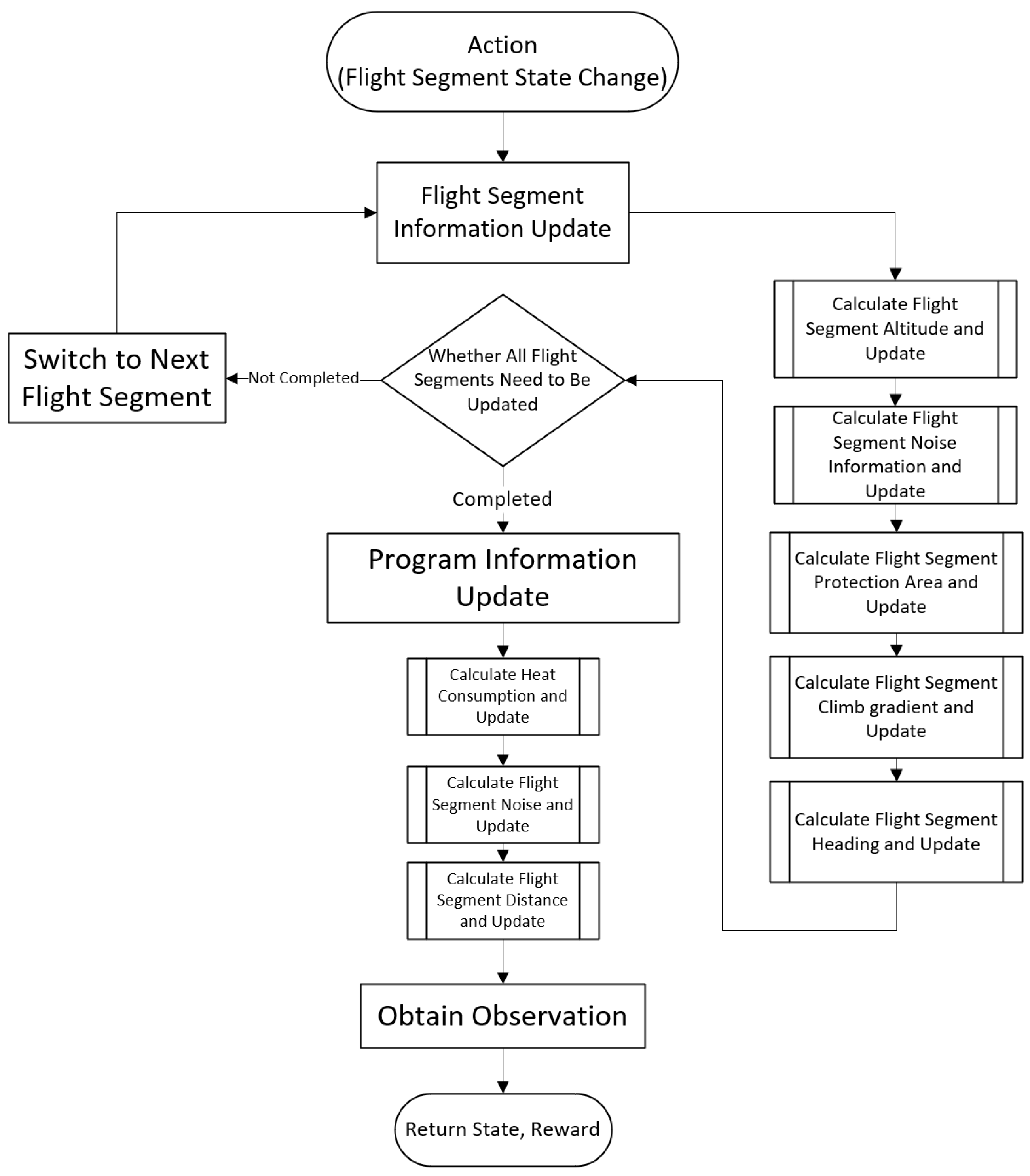
Based on the reward count obtained from the reward curve, as illustrated in Figure 7, it can be observed that the reward function exhibits continuous variation. Furthermore, it has been trained over $3\times {10}^6$ iterations, indicating that the configuration of the reward function is not capable of fully meeting the task requirements.

Reward Function 2:

The optimization objectives of the flight procedure have been further adjusted. Compared to the first version, the design has eliminated the economic objective and focuses on three aspects: safety, simplicity, and noise. Additionally, the safety reward has been normalized, while the normalization setting for the simplicity reward has been removed. The mathematical expression of the reward function is Equation (28):

$$\mathrm{reward}={\mathrm{reward}}_{\mathrm{safe}}+{\mathrm{reward}}_{\mathrm{simply}}+{\mathrm{reward}}_{\mathrm{noise}}$$

(28)

The safety reward in the updated version is expressed as follows (Equation (29)):

$${\mathrm{reward}}_{\mathrm{safe}}={\displaystyle \frac{-S_5-S_6+S_1+S_2+S_3+S_4}{4}}$$

(29)

where $S_1,S_2,S_3,S_4$ represent positive safety factors (such as safety zone distances), and $S_5,S_6$ represent negative risk factors (such as proximity to obstacles). The original version of the equation was $-S_5-S_6+S_1+S_2+S_3+S_4$. In the revised version, a normalization factor of 4 has been introduced to refine the safety components, enabling a more nuanced evaluation of the reward based on minor variations in the parameters.

The simplicity reward is defined as Equation (30), where $S_{\mathrm{simply}}$ can be found in Equation (15).

$${\mathrm{reward}}_{\mathrm{simply}}=S_{\mathrm{simply}}$$

(30)

The noise reward is expressed as Equation (26), which remains unchanged from the previous version.

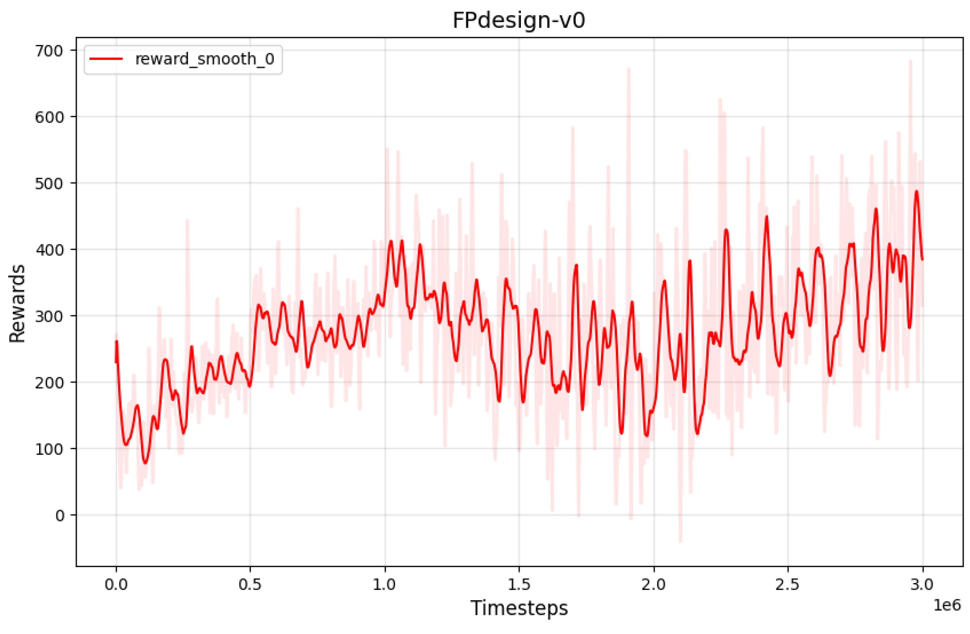
The reward function curve is illustrated in Figure 8. It can be observed that the initial high reward indicates that the strategy is well adapted to the environment, while the mid-stage descent may be related to conflicts among multiple objectives. The late-stage stabilization at a lower level suggests that the strategy has converged, but the desired performance has not been fully achieved.

Reward Function 3:

The third version of the reward function represents a significant improvement and expansion over the second version, aiming to optimize the performance of the flight procedure more comprehensively while enhancing adaptability to complex environmental constraints. The second version of the reward function primarily focused on three aspects: safety, simplicity, and noise control. In this version, the simplicity reward was calculated based on the turning angle, without differentiating between angle and distance simplicity, and it lacked a clear penalty for boundary violations. The third version refines the simplicity objectives by explicitly separating them into angle simplicity and distance simplicity, optimizing both turning angles and segment distances. This refinement significantly enhances the specificity and interpretability of the rewards. The reward function and the definitions of its variables (including their value ranges) are summarized in Equation (31) and

Table 5. Multi-objective optimization reward indicators and their value ranges.

Reward	Definition	Value Range
$r_{\mathrm{safe}}$	Safety reward, determined by the information of obstacles and the distance from the current aircraft to the obstacle.	0–1
$r_{sp\_a}$	Angle efficiency reward, determined by the current route selection and the three turning angles of the aircraft.	0–3
$r_{sp\_l}$	Distance efficiency reward, determined by the distance information and the length of the procedure from the current aircraft to the destination.	0–3
$r_{\mathrm{noise}}$	Environmental noise reward, determined by the negative reward of noise.	0–1

, respectively:

$$reward=\left\{\begin{array}{cc}0\hfill & S_{18}=1\hfill \\ r_{\mathrm{safe}}+r_{s\_l}+r_{sp\_a}+r_{\mathrm{noise}}\hfill & S_{18}=0\hfill \end{array}\right.$$

(31)

The safety reward $r_{\mathrm{safe}}$ is derived from Equation (32), where $r_{\mathrm{safe}}$ takes values between 0 and 1. The previous four states are related to flight disturbance information, with no reward values for obstacles. $S_5$ and $S_6$ represent the changes in the pitch and roll angles of the flight segment. If there are deviations in the pitch and roll angles, a penalty is applied.

$$r_{\mathrm{safe}}={\displaystyle \frac{S_1+S_2+S_3+S_4-S_5-S_6}{4}}$$

(32)

The angle simplicity reward $r_{\mathrm{sp}\_\mathrm{a}}$ is determined by the three angles affected by the current selected flight path, denoted as $S_{10},S_{11},S_{12}$. A turn angle is considered part of a straight departure procedure if it is less than 120 degrees, thus the setting state value must be less than 0.66 to obtain the angle simplicity reward. The calculation method is given by Equation (33), and the formula for the angle simplicity reward is expressed as:

$$\left\{\begin{array}{c}{r}_{\mathrm{sp}\_\mathrm{a}1}=1-S_{10}\hfill \\ r_{\mathrm{sp}\_\mathrm{a}2}=1-S_{11}\hfill \\ r_{\mathrm{sp}\_\mathrm{a}3}=1-S_{12}\hfill \end{array}\right.$$

(33)

$$r_{\mathrm{sp}\_\mathrm{a}}=r_{\mathrm{sp}\_\mathrm{a}1}+r_{\mathrm{sp}\_\mathrm{a}2}+r_{\mathrm{sp}\_\mathrm{a}3}$$

(34)

The distance simplicity reward $r_{\mathrm{sp}\_1}$ is primarily determined by $S_{13}$, $S_{14}$, and $S_{18}$. When the boundary flag $S_{18}$ is set to 1, the total value of the reward function is directly set to 0, representing the maximum negative reward. When the boundary flag $S_{18}$ is 0, and the calculated value of $S_{13}$ is positive, the value for $r_{\mathrm{sp}\_1}$ is computed as twice the value of $S_{13}$. Empirically, this encourages the strategy to explore within a limited distance. Additionally, when the state value $S_{14}$ (representing the total procedure length) is less than 0.3, an additional reward based on $S_{14}$ is added, as shown in Equation (35):

$$r_{\mathrm{sp}\_1}=\left\{\begin{array}{cc}{S}_{13}\times 2\hfill & \mathrm{if}{S}_{14}\ge 0.3\hfill \\ \left(S_{13}\times 2+(0.3-S_{14})\times 10\right)\hfill & \mathrm{if}{S}_{14}<0.3\hfill \end{array}\right.$$

(35)

The environmental reward $r_{\mathrm{noise}}$ is derived from the negative reward of noise. It remains an empirical formula, calculated by dividing the total noise N, updated by the procedure, by 10,000, as shown in Equation (36):

$$r_{\mathrm{noise}}=-{\displaystyle \frac{N}{10000}}$$

(36)

where N is calculated as shown in Equation (27), based on the environmental model detailed in the Problem Formulation section.

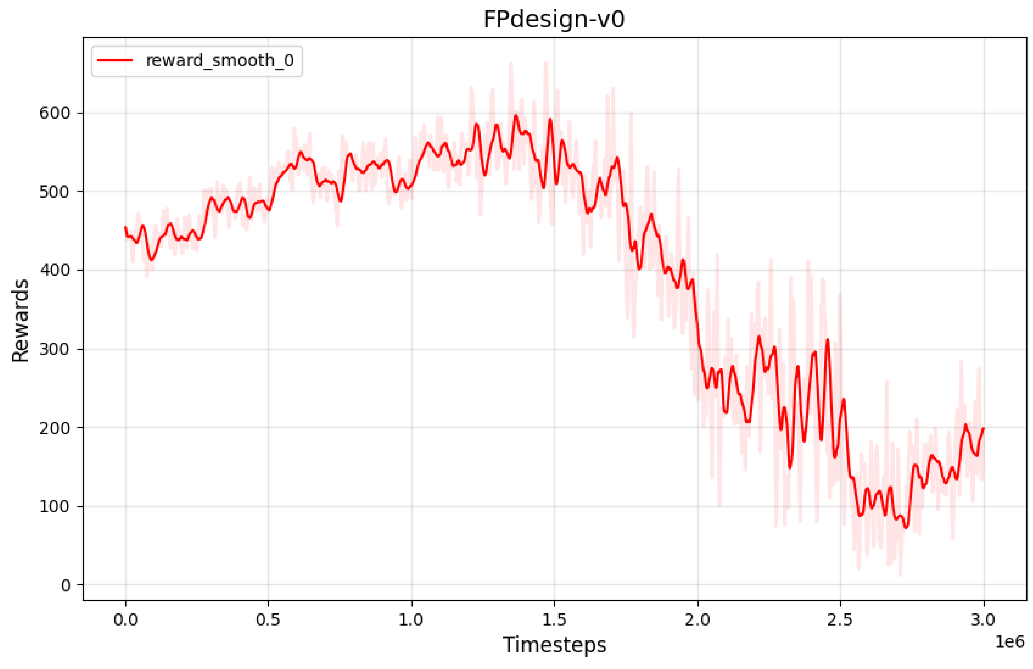
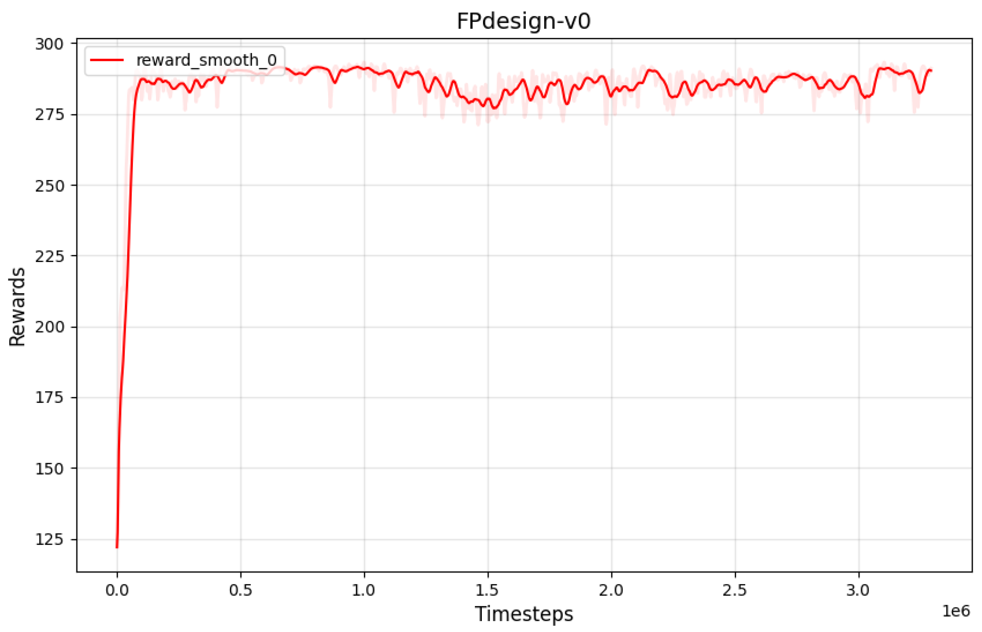
The reward function curve is shown below. As seen from Figure 9, the curve converges around 50,000 iterations. The reward curve demonstrates an overall upward trend with oscillations close to a peak value, indicating that the model has learned an effective strategy. The algorithm and environmental adjustments can be considered complete.

The results of the three reward functions:

The models trained with the three aforementioned reward functions were each used to sample 50 independent trajectories, and the proportion of fully safe flight procedures among these 50 trajectories was statistically analyzed. Subsequently, the fully safe flight procedures were subjected to flight simulation tests using the BlueSky simulation platform, where the average fuel consumption and flight time were recorded. The experimental results are presented in

Table 6. The experimental results of three different reward functions.

	Safety Procedure Ratio	Average Fuel Consumption (kg)	Average Flight Time (s)
Reward 1	8%	295.7	1087
Reward 2	16%	235.7	823
Reward 3	46%	150.3	523

. In BlueSky, the aircraft type employed was the A320, with a speed setting of 200 kt, which falls within the permissible departure procedure speed range for Category C aircraft.

BlueSky is an open-source air traffic management simulation platform that provides a flexible and extensible environment, supporting the integration of OpenAP and BADA aerodynamic data packages for flight simulation validation. The platform offers statistical functionalities for fuel consumption and flight time [36].

Table 6 demonstrates that reward function 3, which was carefully designed, achieves the best performance, with a safe procedure ratio of 46%, an average fuel consumption of 150.3 kg, and an average flight time of 523 seconds. The proportion of safe procedures is significantly higher than those obtained with the other two reward functions. This improvement is attributed to the stable state achieved by the model trained with reward function 3 during the later training phase, as illustrated in Figure 9. In contrast, the models trained with reward functions 1 and 2 did not converge, resulting in unstable outputs and lower safe procedure ratios. Additionally, it was observed that even with the model using reward function 3, approximately half of the sampled flight procedures failed to meet safety standards, highlighting a direction for future improvement.

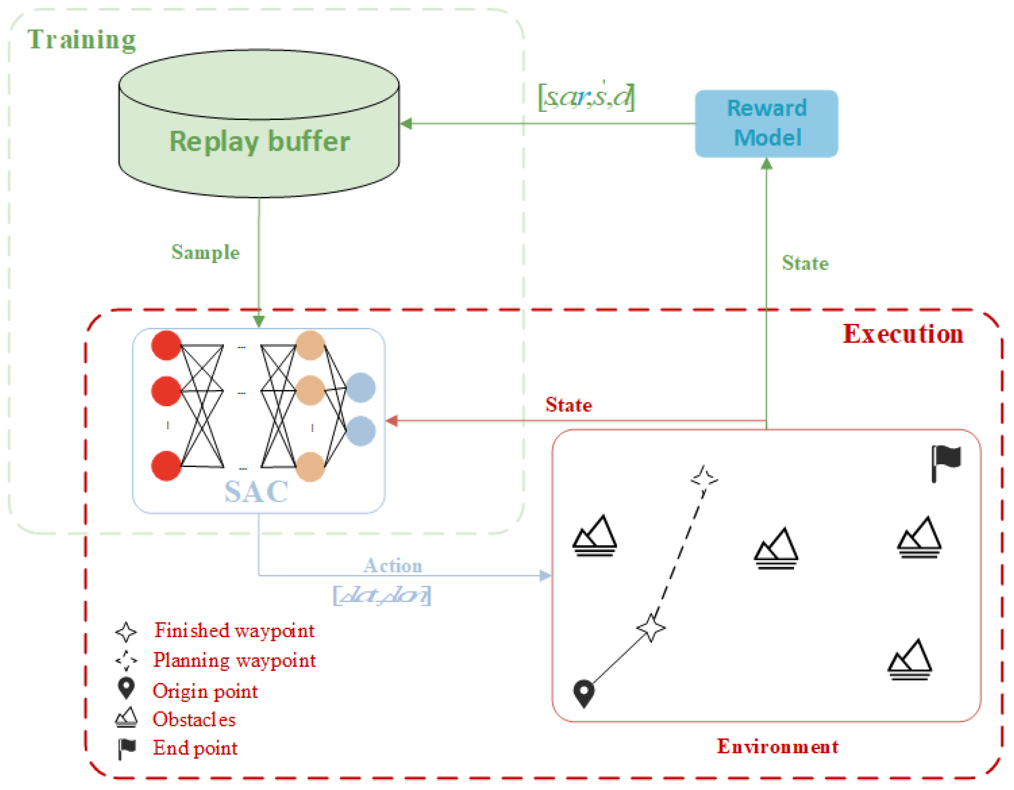
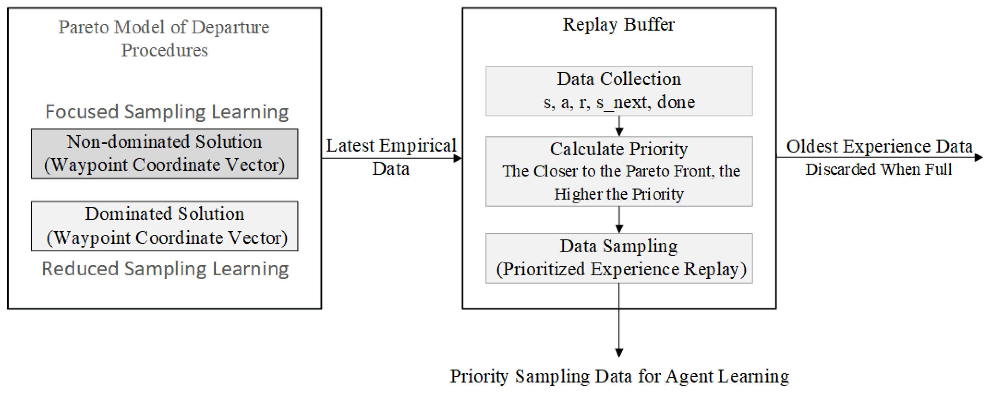
4.2.2. Pareto-Based Replay Buffer Sampling

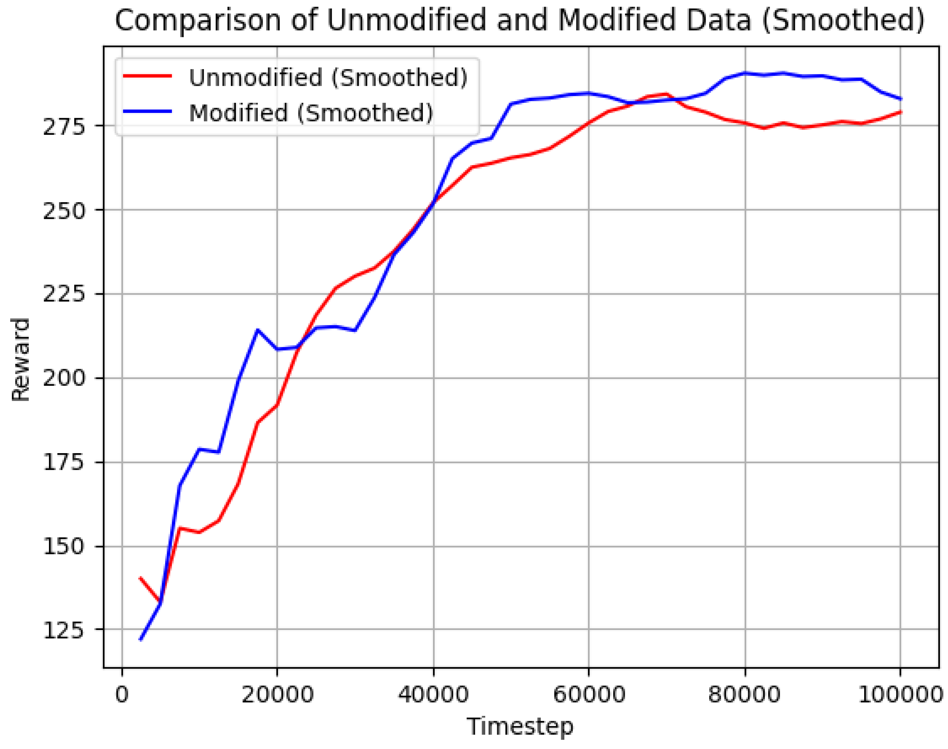
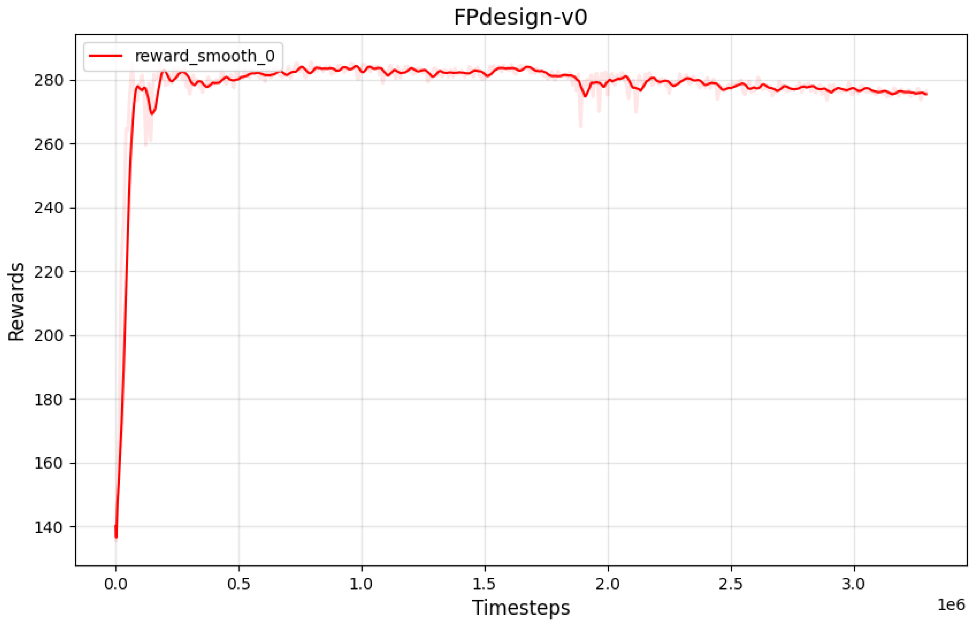
The experiment includes two comparison groups: one group applies the soft actor–critic (SAC) algorithm with an unmodified sampling mechanism, while the other employs an improved replay buffer within the SAC algorithm [37]. The convergence curve of the original SAC reward is shown in Figure 9, while the reward curve of SAC with the improved replay buffer and dynamic learning rate adjustment is shown in Figure 10. The reward curve of the improved SAC converges in a significantly shorter number of time steps and does not exhibit the slight decline in peak values observed in the later stages of training with the original SAC algorithm. Furthermore, dynamic learning rate adjustment helps maintain the variance of the reward curve within a reasonable range.

By comparing the convergence curves of the reward functions for both algorithms, as illustrated in Figure 11, it is observed that the convergence speeds are comparable. However, the reward curve obtained from the improved algorithm reaches peak values closer to the theoretically optimal strategy during convergence. While this method results in an increase in the variance of the reward curve, the dynamic learning rate adjustment strategy effectively keeps it within an acceptable range.

Through experimental evaluation, the average score of the improved SAC reward shows a 4% increase compared to the original SAC reward, as illustrated in

Table 7. Comparison of original and improved SAC reward scores.

Method	Original SAC Average Reward	Improved SAC Average Reward	Comparison
Score	275.3	285.5	+4%

below. Moreover, the optimization speed of the improved method is 28.6% faster than the original approach, as shown in Figure 12.

From the visualization results in Figure 13, it can be observed that the improved SAC algorithm demonstrates more significant effects in terms of optimization speed and results. This indicates the effectiveness of scalarizing the reward function in multi-objective optimization and demonstrates the efficacy of the Pareto-optimal prioritized experience replay sampling strategy in enhancing algorithm performance.

Furthermore, we conducted 50 independent samplings using the SAC algorithm with the improved sampling strategy and calculated the proportion of absolutely safe flight procedures. These procedures were then subjected to flight simulation tests using the BlueSky simulation platform, where the average fuel consumption and flight time were recorded. The experimental results are presented in

Table 8. Comparison of original and improved SAC algorithm performance.

Algorithm	Safety Procedure Ratio	Average Fuel Consumption (kg)	Average Flight Time (s)
Original SAC	46%	150.3	523
Improved SAC	56%	137.2	500

. The improved SAC algorithm demonstrates significant enhancements in the safety procedure ratio, average fuel consumption, and average flight time. Specifically, the safety procedure ratio increased from 46% to 56%, the average fuel consumption decreased from 150.3 kg to 137.2 kg, and the average flight time was reduced from 523 s to 500 s. These findings indicate that the improved SAC algorithm exhibits superior performance in multi-objective optimization.

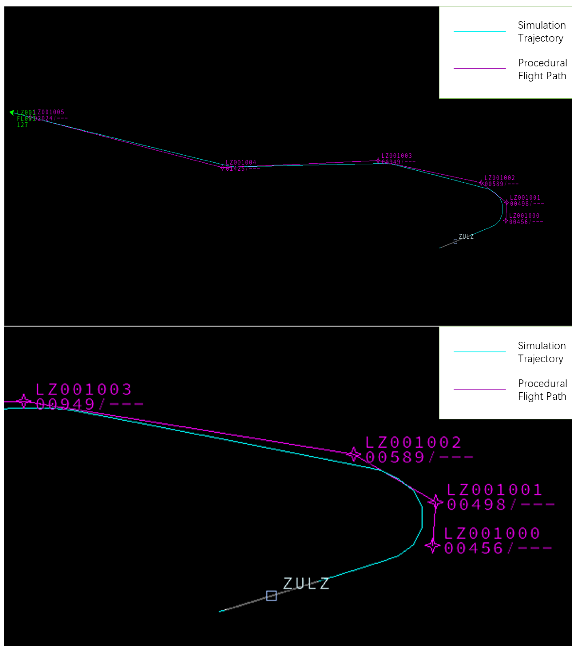
The visualization results of the improved SAC algorithm in BlueSky are presented in Figure 13, with a detailed comparison shown in Figure 14. The figures demonstrate that the procedures designed by the proposed method can be accurately executed by the flight simulator, highlighting the practical value of the approach presented in this study.

5. Conclusions and Future Work

5.1. Conclusions

This study introduces a novel reinforcement learning (RL) framework for intelligent flight procedure design, incorporating multi-objective optimization to concurrently address safety, simplicity, and environmental sustainability. By leveraging the soft actor–critic (SAC) algorithm, enhanced with a Pareto-based prioritized experience replay sampling strategy, the framework successfully trained an intelligent agent capable of autonomously optimizing performance-based navigation (PBN) departure procedures. The proposed approach was validated through the design and optimization of a departure procedure for Luzhou Airport, demonstrating its feasibility and effectiveness using the BlueSky open-source flight simulation platform. Experimental results indicate that the optimized procedures effectively balance the conflicting objectives of safety (e.g., obstacle avoidance), simplicity (e.g., reduced path length and turning angles), and environmental impact (e.g., noise reduction). Compared to the baseline SAC algorithm, the improved method achieves a 28.6% increase in convergence speed and a 4% improvement in overall performance across the multi-objective metrics, highlighting the effectiveness of the Pareto-optimal sampling strategy and dynamic learning rate adjustments.

The primary innovation of this work lies in the integration of RL with Pareto-based multi-objective optimization, addressing the limitations of traditional flight procedure design methods that heavily rely on expert experience and static guidelines. Through meticulous reward engineering, we developed a comprehensive reward function that quantifies and balances safety, simplicity, and noise impact, thereby guiding the agent toward optimal solutions. Incorporating a multi-objective sampling strategy substantially enhances sampling efficiency, addressing inherent limitations of uniform sampling in traditional reinforcement learning frameworks. The optimized procedures, validated through successful execution in the BlueSky simulation platform, demonstrate strong practical applicability. This study provides a robust foundation for advancing the automation and optimization of flight procedure design, with potential implications for improving airspace efficiency and sustainability in modern aviation.

Despite these advancements, several limitations persist. The validation of procedure rationality primarily relies on simulated flight trajectories, focusing on safety, simplicity, and environmental impact, while other critical factors, such as pilot workload and air traffic control constraints, remain underexplored. Furthermore, the reliance on BlueSky’s simplified kinematic models constrains the fidelity of real-world force dynamics, underscoring the need for validation using more advanced simulators. Additionally, for complex scenarios, rapid simulations alone may be insufficient to ensure robust validation, suggesting that flight trials with real aircraft could be necessary to confirm the procedures’ practical applicability. The algorithm’s optimization is currently tailored to PBN departure procedures, and its adaptability to approach or missed approach procedures has yet to be validated, given the distinct environmental complexities involved. Lastly, while dynamic learning rate adjustment enhances the algorithm’s performance, it may not fully mitigate reward variance across all scenarios, indicating a need for further refinement.

5.2. Future Work

Building on the findings and limitations of this study, several avenues for future research are proposed to enhance the proposed framework and its practical utility:

Future work should incorporate high-fidelity flight simulators that account for real-world aerodynamic forces and operational constraints. This would improve the credibility and robustness of validation results, going beyond the capabilities of BlueSky. By simulating more complex dynamics, we can better assess the effectiveness of the flight procedure design in various real-world conditions.

The Pareto-optimal prioritized experience replay strategy, while effective, increases reward variance in certain scenarios. Although dynamic learning rate adjustments help mitigate this issue, alternative approaches—such as adaptive priority mechanisms or hybrid sampling strategies—could be explored to achieve more stable and optimal performance. Further refinement of the reward function and learning dynamics will also contribute to a more resilient algorithm.

The current framework is tailored to PBN departure procedures. Extending the multi-objective optimization environment and RL algorithm to accommodate approach and missed approach procedures would broaden its applicability. Leveraging the experience gained from this study, a more versatile design tool could be developed, applicable to a wider range of flight procedures.

The present modeling of departure procedures may not encompass all relevant factors (e.g., weather variations, airspace capacity) or be fully adaptable to other procedure types. Future efforts should aim to develop a more holistic optimization framework, potentially culminating in an autonomous flight procedure design system capable of replacing human designers. Incorporating more variables, such as operational disruptions and real-time adjustments, will enhance the robustness of the framework.

In summary, this research represents a significant step toward intelligent flight procedure design by demonstrating the potential of RL and multi-objective optimization. Addressing the identified shortcomings through these future directions will further advance the field, paving the way for fully autonomous and sustainable aviation solutions.

References

1. Pamplona, D.A.; de Barros, A.G.; Alves, C.J. Performance-based navigation flight path analysis using fast-time simulation. Energies 2021, 14, 7800. [Google Scholar] [CrossRef]
2. Salgueiro, S.; Hansman, R.J. Potential Safety Benefits of RNP Approach Procedures. In Proceedings of the 17th AIAA Aviation Technology, Integration, and Operations Conference, Denver, CO, USA, 5–9 June 2017; p. 3597. [Google Scholar]
3. Muller, D.; Uday, P.; Marais, K. Evaluation of the potential environmental benefits of RNAV/RNP arrival procedures. In Proceedings of the 11th AIAA Aviation Technology, Integration, and Operations (ATIO) Conference, Including the AIAA Balloon Systems Conference and 19th AIAA Lighter-Than, Virginia Beach, VA, USA, 20–22 September 2011; p. 6932. [Google Scholar]
4. López-Lago, M.; Serna, J.; Casado, R.; Bermúdez, A. Present and future of air navigation: PBN operations and supporting technologies. Int. J. Aeronaut. Space Sci. 2020, 21, 451–468. [Google Scholar] [CrossRef]
5. Tian, Y.; Wan, L.; Chen, C.h.; Yang, Y. Safety assessment method of performance-based navigation airspace planning. J. Traffic Transp. Eng. (Engl. Ed.) 2015, 2, 338–345. [Google Scholar] [CrossRef]
6. Zhu, L.; Wang, J.; Wang, Y.; Ji, Y.; Ren, J. DRL-RNP: Deep reinforcement learning-based optimized RNP flight procedure execution. Sensors 2022, 22, 6475. [Google Scholar] [CrossRef]
7. Misra, S. Simulation analysis of the effects of performance-based navigation on fuel and block time efficiency. Int. J. Aviat. Aeronaut. Aerosp. 2020, 7, 7. [Google Scholar] [CrossRef]
8. Otero, E.; Tengzelius, U.; Moberg, B. Flight Procedure Analysis for a Combined Environmental Impact Reduction: An Optimal Trade-Off Strategy. Aerospace 2022, 9, 683. [Google Scholar] [CrossRef]
9. Guo, D.; Huang, D. PBN operation advantage analysis over conventional navigation. Aerosp. Syst. 2021, 4, 335–343. [Google Scholar] [CrossRef]
10. Zu, W.; Yang, H.; Liu, R.; Ji, Y. A multi-dimensional goal aircraft guidance approach based on reinforcement learning with a reward shaping algorithm. Sensors 2021, 21, 5643. [Google Scholar] [CrossRef]
11. Razzaghi, P.; Tabrizian, A.; Guo, W.; Chen, S.; Taye, A.; Thompson, E.; Bregeon, A.; Baheri, A.; Wei, P. A survey on reinforcement learning in aviation applications. Eng. Appl. Artif. Intell. 2024, 136, 108911. [Google Scholar] [CrossRef]
12. Quadt, T.; Lindelauf, R.; Voskuijl, M.; Monsuur, H.; Čule, B. Dealing with Multiple Optimization Objectives for UAV Path Planning in Hostile Environments: A Literature Review. Drones 2024, 8, 769. [Google Scholar] [CrossRef]
13. Yang, F.; Huang, H.; Shi, W.; Ma, Y.; Feng, Y.; Cheng, G.; Liu, Z. PMDRL: Pareto-front-based multi-objective deep reinforcement learning. J. Ambient Intell. Humaniz. Comput. 2023, 14, 12663–12672. [Google Scholar] [CrossRef]
14. Zhang, Y.; Zhao, W.; Wang, J.; Yuan, Y. Recent progress, challenges and future prospects of applied deep reinforcement learning: A practical perspective in path planning. Neurocomputing 2024, 608, 128423. [Google Scholar] [CrossRef]
15. Xia, Q.; Ye, Z.; Zhang, Z.; Lu, T. Multi-objective optimization of aircraft landing within predetermined time window. SN Appl. Sci. 2022, 4, 198. [Google Scholar] [CrossRef]
16. Gardi, A.; Sabatini, R.; Ramasamy, S. Multi-objective optimisation of aircraft flight trajectories in the ATM and avionics context. Prog. Aerosp. Sci. 2016, 83, 1–36. [Google Scholar] [CrossRef]
17. Ribeiro, M.; Ellerbroek, J.; Hoekstra, J. Using reinforcement learning to improve airspace structuring in an urban environment. Aerospace 2022, 9, 420. [Google Scholar] [CrossRef]
18. To70. Flight Procedure Design. Available online: https://to70.com/flight-procedure-design/ (accessed on 17 March 2025).
19. SKYbrary. Airspace and Procedure Design. Available online: https://skybrary.aero/articles/airspace-and-procedure-design (accessed on 17 March 2025).
20. Israel, E.; Barnes, W.J.; Smith, L. Automating the design of instrument flight procedures. In Proceedings of the 2020 Integrated Communications Navigation and Surveillance Conference (ICNS), Herndon, VA, USA, 8–10 September 2020; p. 3D2-1. [Google Scholar]
21. Lai, Y.Y.; Christley, E.; Kulanovic, A.; Teng, C.C.; Björklund, A.; Nordensvärd, J.; Karakaya, E.; Urban, F. Analysing the opportunities and challenges for mitigating the climate impact of aviation: A narrative review. Renew. Sustain. Energy Rev. 2022, 156, 111972. [Google Scholar] [CrossRef]
22. Schaul, T.; Quan, J.; Antonoglou, I.; Silver, D. Prioritized experience replay. arXiv 2015, arXiv:1511.05952. [Google Scholar]
23. Hessel, M.; Modayil, J.; Van Hasselt, H.; Schaul, T.; Ostrovski, G.; Dabney, W.; Horgan, D.; Piot, B.; Azar, M.; Silver, D. Rainbow: Combining Improvements in Deep Reinforcement Learning. In Proceedings of the AAAI Conference on Artificial Intelligence, New Orleans, LA, USA, 2–7 February 2018; Volume 32. [Google Scholar]
24. Zhang, S.; Sutton, R.S. A deeper look at experience replay. arXiv 2017, arXiv:1712.01275. [Google Scholar]
25. Clavera, I.; Rothfuss, J.; Schulman, J.; Fujita, Y.; Asfour, T.; Abbeel, P. Model-based reinforcement learning via meta-policy optimization.
26. Yin, H.; Pan, S. Knowledge transfer for deep reinforcement learning with hierarchical experience replay. In Proceedings of the AAAI Conference on Artificial Intelligence, San Francisco, CA, USA, 4–9 February 2017; Volume 31. [Google Scholar]
27. Pathak, D.; Agrawal, P.; Efros, A.A.; Darrell, T. Curiosity-driven exploration by self-supervised prediction. In Proceedings of the International Conference on Machine Learning, PMLR, Sydney, Australia, 6–11 August 2017; pp. 2778–2787. [Google Scholar]
28. Kapturowski, S.; Ostrovski, G.; Dabney, W.; Quan, J.; Munos, R. Recurrent Experience Replay in Distributed Reinforcement Learning. In Proceedings of the International Conference on Learning Representations, New Orleans, LA, USA, 6–9 May 2019. [Google Scholar]
29. Yang, J.; Sun, Y.; Chen, H. Differences Between Traditional Navigation and PBN Departure Procedures and Automation of Protected Area Drawing Using AutoLISP. Mod. Comput. 2015, 56–59. [Google Scholar]
30. Dai, F. Flight Procedure Design; Tsinghua University Press: Beijing, China; Beijing Jiaotong University Press: Beijing, China, 2017. [Google Scholar]
31. Abeyratne, R. Article 38 Departures from International Standards and Procedures. In Proceedings of the Convention on International Civil Aviation: A Commentary; Springer: Cham, Switzerland, 2014; pp. 417–464. [Google Scholar] [CrossRef]
32. Dao, G.; Lee, M. Relevant experiences in replay buffer. In Proceedings of the 2019 IEEE Symposium Series on Computational Intelligence (SSCI), Xiamen, China, 6–9 December 2019; pp. 94–101. [Google Scholar]
33. Lampariello, L.; Sagratella, S.; Sasso, V.G.; Shikhman, V. Scalarization via utility functions in multi-objective optimization. arXiv 2024, arXiv:2401.13831. [Google Scholar]
34. Yuping, H.; Weixuan, L.; Zuhuan, X. Comparative analysis of deep learning framework based on TensorFlow and PyTorch. Mod. Inf. Technol. 2020, 4, 80–82. [Google Scholar]
35. Goodfellow, I.; Bengio, Y.; Courville, A.; Bengio, Y. Deep Learning; MIT Press: Cambridge, MA, USA, 2016; Volume 1. [Google Scholar]
36. Hoekstra, J.M.; Ellerbroek, J. Bluesky ATC simulator project: An open data and open source approach. In Proceedings of the 7th International Conference on Research in Air Transportation, Philadelphia, PA, USA, 20–24 June 2016; Volume 131, p. 132. [Google Scholar]
37. Liu, J.; Liu, Y.; Luo, X. Research Progress in Deep Learning. Appl. Res. Comput. 2014, 31. [Google Scholar]
Figure 1. Straight-out departure protected area.
Aerospace 12 00451 g001
Figure 2. Obstacle identification surface.
Aerospace 12 00451 g002
Figure 3. Framework for reinforcement-learning-based flight procedure design.
Aerospace 12 00451 g003
Figure 4. The Pareto model of multi-objective optimization problem in flight procedure design.
Aerospace 12 00451 g004
Figure 5. Schematic diagram of the replay buffer structure.
Aerospace 12 00451 g005
Figure 6. The process of procedure information update.
Aerospace 12 00451 g006
Figure 7. The model reward curve of reward function 1.
Aerospace 12 00451 g007
Figure 8. The model reward curve of reward function 2.
Aerospace 12 00451 g008
Figure 9. The model reward curve of reward function 3.
Aerospace 12 00451 g009
Figure 10. The reward curve of the improved SAC.
Aerospace 12 00451 g010
Figure 11. Reward curve comparison chart.
Aerospace 12 00451 g011
Figure 12. Comparison of convergence speed before and after improvement.
Aerospace 12 00451 g012
Figure 13. Visualization results of the improved SAC algorithm.
Aerospace 12 00451 g013
Figure 14. Procedure and flight path render in BlueSky.
Aerospace 12 00451 g014