Design and Cushioning Performance Analysis of Spherical Tensegrity Structures

Abstract

This study aims to design a novel combined spherical tensegrity structure and evaluate its cushioning performance to offer a new option for a planetary exploration landing mechanism. Initially, based on the circumferential assembling method, a “class II” spherical tensegrity structure was constructed using the square frustum tensegrity unit as the basic element. Then, the equilibrium equations for the structure were formulated in accordance with the principle of virtual work to confirm the self-equilibrium of the tensegrity configuration, and the stability of the designed structure was assessed by determining the type of the tensegrity structure according to the Maxwell criterion and the character of the stiffness matrix. Subsequently, the simulation and analysis of the compressive stiffness of the structure under different parameters were carried out based on the finite element analysis method. The landing collision was simulated by using dynamic software to analyze the influence of the structure parameters on the cushioning performance. Finally, an experimental model was built to verify the above analysis, which demonstrates that the designed spherical tensegrity structure offered a large loading space and great cushioning performance.

1. Introduction

Tensegrity structure is a type of cable-bar tensile structure consisting of discontinuous compressed bars and continuous tensioned cables [1]. As a kind of spatial structure with a simple structure, lightweight, beautiful appearance, and strong expansibility, it has been widely used in architecture, aerospace, mechanical engineering, art, and biology since the middle of the 20th century [2,3,4]. Tensegrity structures combine lightweight design, flexibility, robustness, and safety in a unique way [5,6,7], which are particularly suitable for constructing collaborative robots and soft robots [8,9]. Moreover, tensegrity structures exhibit excellent mobility and impact resistance, which has led to extensive research on and applications of tensegrity robots in fields such as planetary exploration and bionics [2,3,10,11,12,13,14].

Spherical tensegrity does not mean that the structure has a smooth spherical external structure, but rather that its overall shape approximates a sphere [15,16,17,18]. NASA initiated the “Super Ball” project to develop spherical robots based on the classic six-bar tensegrity structure and conducted research on their structural and motion performance [19,20,21]. Bohm et al. [22,23] replaced the bar units in traditional tensegrity with two rigid and unconnected curved surface units to increase the internal space of the spherical tensegrity structure. Kim et al. [24] designed a twelve-bar spherical tensegrity robot “T12-R” based on a rhombic octahedron. The geometric shape makes it more suitable for high-speed rolling, and it can move in a straight line. Zhang et al. [25,26] constructed spherical tensegrity structures based on truncated regular polyhedral and analyzed the self-equilibrium and self-stability of truncated regular tetrahedron, hexahedron, and octahedron structures. However, current spherical tensegrity structures have drawbacks such as a single configuration and limited flexibility in altering the internal load-bearing space of the devices.

In planetary exploration missions, spherical tensegrity structures can enable soft landings on the surface of planets, effectively reducing impact forces on internal components. Therefore, the cushioning ability of tensegrity structures plays a critical role in ensuring safe landings. Lee-Huang Chen et al. [27,28] conducted collision dynamics analysis on six-bar spherical tensegrity robots and utilized simulation software to simulate the collision between the tensegrity robots and the ground, considering two mass distribution conditions. Schroeder [29] designed a truncated icosahedron tensegrity structure and discussed collision modeling methods, which are validated through rigorous calculations and simulations. Gebara et al. [30] designed an ocean lander based on a truncated octahedron tensegrity structure, which demonstrates the capability to overcome liquid surface tension while sustaining high-altitude impact loads. Zhao et al. [31] investigated the impact of various factors, including topological structures, bar mass, cable mass, and payload mass, on the maximum acceleration of the payload during collision. Spherical tensegrity structures have received significant attention in recent years. However, they still face challenges such as limited structural forms, restricted loading space, and inadequate cushioning performance.

This paper constructs a novel spherical tensegrity structure utilizing a small oblique square half-truncated prism as the assembling shape. The structure is assembled using six four-bar frustum basic units, designed for “class II” [32,33] circumferential assembling. The equilibrium equations of the structure are derived using the principle of virtual work. This approach can be used to determine the internal forces of the elements within the structure and assess its self-equilibrium. Then, the stability of the structure is assessed by analyzing the self-stress modes, displacement modes, and the positive definiteness of the tangent stiffness matrix of the structure. Simulation is conducted to study the impact of different structural parameters on the compressive stiffness and cushioning performance of the structure. The simulation results are validated through experiments with physical models.

2. Design and Self-Equilibrium Analysis of Spherical Tensegrity Structures

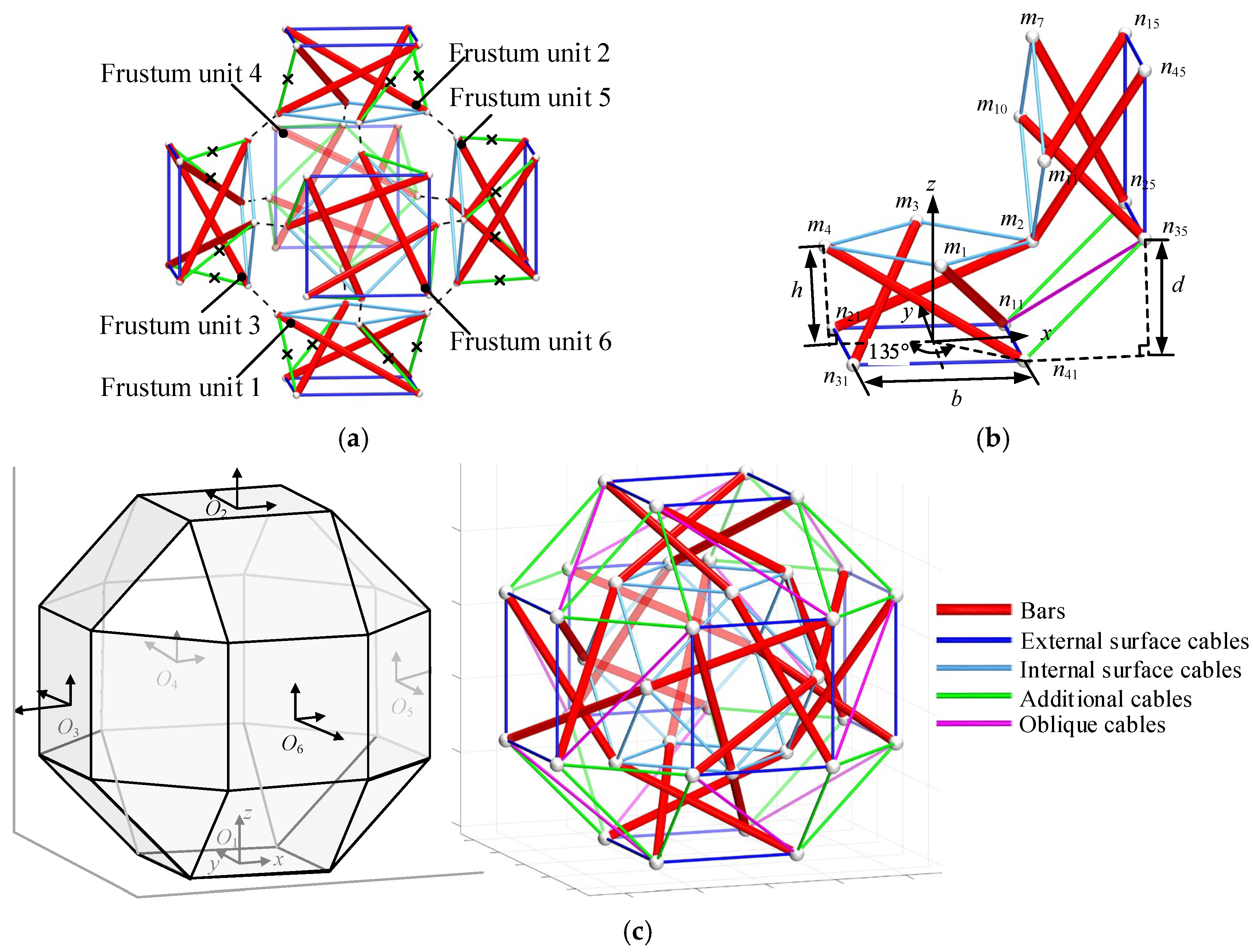
2.1. Design of the Spherical Tensegrity Structure

In order to ensure the stiffness and loading capacity of the tensegrity structure, the type of structure is classified as a “class II”, characterized by two bars fixed at each node. The assembling process is illustrated in Figure 1a. Six identical four-bar frustum tensegrity units are arranged circumferentially, the external nodes align with the vertices of a small oblique square half-truncated prism, while the internal nodes align with the vertices of a half-truncated cube. The original diagonal cables of the four-bar unit are replaced with alternative cables.

The local connection between two four-bar units is depicted in Figure 1b. The internal rotation angle of the unit, defined as the angle between the projections of the nodes at both ends of the bars onto the base and the lines connecting the centroid of the base, is 135°. Additionally, the upper and lower surfaces of each unit are square, with their diagonals perpendicular to each other. The external surface nodes are connected by additional cables and oblique cables, while the internal surface nodes are connected by bars.

The components of the structure can be divided into five categories, bar, external surface cables, additional cables, internal surface cables, and oblique cables, the number of each component is shown in

Table 1. Number of components.

Components	Number of Components
bars	24
external surface cables	24
internal surface cables	24
additional cables	24
oblique cables	12
external surface nodes	24
internal surface nodes	12

. The external surfaces of the six units coincide with the six square surfaces of the small oblique square half-truncated prism. A spherical tensegrity structure consisting of 24 bars and 84 cable components is obtained, as shown in Figure 1c. The nodes on the external and the internal surface of the unit are denoted by n_ij and m_k, respectively, where i (i = 1, 2, 3, 4) indicates the node number within one unit, j (j = 1, 2, …, 6) indicates the unit number, and k (k = 1, 2, …, 12) represents the node number on the internal surface of the unit.

All components are connected at both ends of the nodes. The topology diagram of the cable component connections is shown in Figure 2, where the circles represent the nodes in the structure, while the lines of different colors and types represent the cable components connecting these nodes.

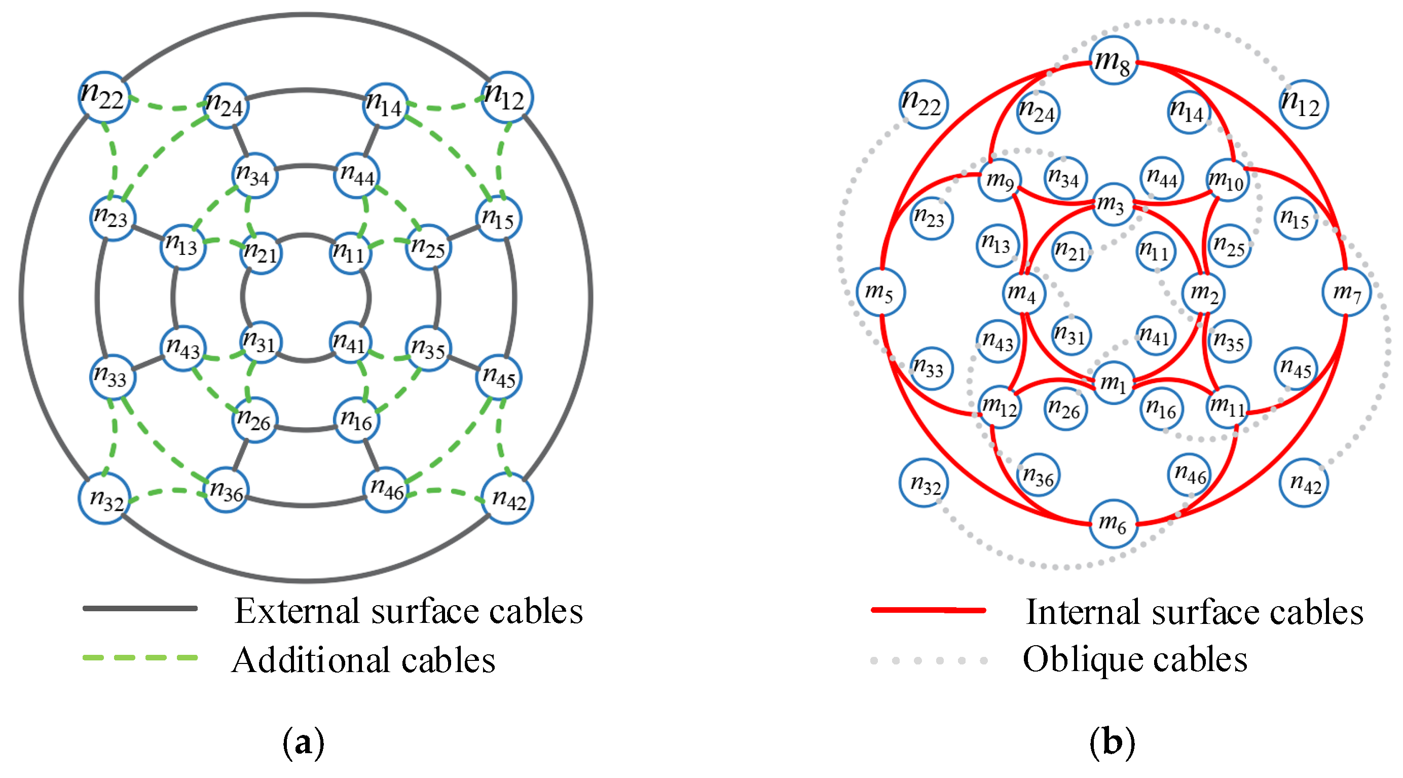
2.2. Establishment of the Geometric Model

As shown in Figure 1b, the length of the external square side of the unit is denoted by b, and the vertical distance between units is expressed as d. The range of the unit height $h\in \left(d/2,d/2+b/2\right)$. An inertial coordinate system O₁ is introduced, which is located at the origin of coordinate system. Using C, the three-dimensional rotation matrix around the z-axis, the coordinates of nodes n_i1 and m_k of basic unit 1 in Figure 1 with respect to the inertial coordinate system can be expressed as:

$${\mathit{n}}_{i1}={\mathit{C}}^{i-1}{\left[\begin{array}{ccc}b/2& b/2& 0\end{array}\right]}^T, i=1, 2, 3, 4$$

(1)

$${\mathit{m}}_k={\mathit{C}}^{k-1}{\left[\begin{array}{ccc}0& -b/2-d+h& h\end{array}\right]}^T, k=1, 2, 3, 4$$

(2)

Here, the vertical distance between units, $d=\sqrt{2}b/2$, is derived from the geometric relationship of the small oblique square half-truncated prism, C represents the rotation matrix fora π/2 counterclockwise rotation around the z-axis, and its expression is:

$$C=\left[\begin{array}{ccc}\cos {\displaystyle \frac{\pi }{2}}& -\sin {\displaystyle \frac{\pi }{2}}& 0\\ \sin {\displaystyle \frac{\pi }{2}}& \cos {\displaystyle \frac{\pi }{2}}& 0\\ 0& 0& 1\end{array}\right]$$

(3)

Then, the local coordinate systems O_j (j = 2, 3, …, 6), located at the geometric centers of the other five external surface squares as shown in Figure 1c, are established. The displacement and the rotational angle of the local coordinate systems O_j with respect to the inertial coordinate system O₁ are expressed as ${\mathit{t}}_j=[\begin{array}{ccc}{x}_j& y_j& z_j\end{array}{]}^T$ and ${\mathit{r}}_j=[\begin{array}{ccc}{\phi }_j& {\gamma }_j& {\theta }_j\end{array}{]}^T$, respectively [34]. The displacement matrix and the rotation matrix of the local coordinate system relative to the inertial coordinate system are expressed as $\mathit{T}=\left[\begin{array}{ccccc}{\mathit{t}}_1& \dots & {\mathit{t}}_j& \dots & {\mathit{t}}_6\end{array}\right]$, and $\mathit{R}=\left[\begin{array}{ccccc}{\mathit{r}}_1& \dots & {\mathit{r}}_j& \dots & {\mathit{r}}_6\end{array}\right]$, respectively. Since the external nodes of the circumferentially spliced spherical tensegrity structure coincide with the vertices of the small oblique truncated cube, T and R can be expressed as:

$$\mathit{T}=\left[\begin{array}{cccccc}0& 0& -(b/2+d)& 0& b/2+d& 0\\ 0& 0& 0& b/2+d& 0& -(b/2+d)\\ 0& b+2d& b/2+d& b/2+d& b/2+d& b/2+d\end{array}\right]$$

(4)

$$\mathit{R}=\left[\begin{array}{cccccc}0& 0& 0& 0& 0& 0\\ 0& 0& 0& \pi /2& 0& 3\pi /2\\ 0& 0& \pi /2& 0& 3\pi /2& 0\end{array}\right]$$

(5)

According to the coordinates of the first frustum unit, the coordinates of the nodes n_ij (i = 1, 2, 3, 4; j = 2, 3, 4, 5, 6) and m_k (k = 5, 6, 7, 8) of the other five basic units, with respect to the inertial coordinate system, can be expressed as:

$${\mathit{n}}_{ij}={\mathit{t}}_j+{\mathit{R}}_j^{zxy}{\mathit{n}}_{i1}$$

(6)

$${\mathit{m}}_k={\mathit{t}}_j+{\mathit{R}}_j^{zxy}{\mathit{m}}_{k-4}$$

(7)

where ${{\mathit{R}}_j}^{zxy}$ is the transformation matrix between the inertial coordinate system and the local coordinate system.

$${\mathit{R}}_j^{zxy}={\mathit{R}}_z\left({\phi }_j\right){\mathit{R}}_x\left({\gamma }_j\right){\mathit{R}}_y\left({\theta }_j\right)$$

(8)

where ${\mathit{R}}_z\left({\phi }_j\right)$ denotes the rotation matrix for a counterclockwise rotation by an angle φ_j around the coordinate axis z, ${\mathit{R}}_x\left({\gamma }_j\right)$ denotes the rotation matrix for a counterclockwise rotation by an angle γ_j around the coordinate axis x, and ${\mathit{R}}_y\left({\theta }_j\right)$ denotes the rotation matrix for a counterclockwise rotation by an angle θ_j around the coordinate axis y.

The coordinates of the internal nodes m_k (k = 9, 10, 11, 12) can be expressed as:

$${\mathit{m}}_k={\mathit{C}}^{12-k}\left({\mathit{t}}_3+{\mathit{F}}_3^{zxy}{m}_1\right)$$

(9)

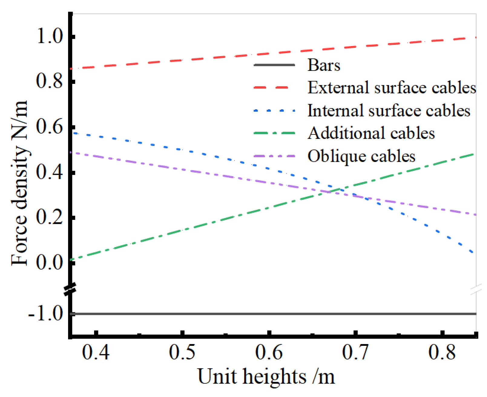
2.3. Self-Equilibrium Analyssssis and Parametric Design of Structure

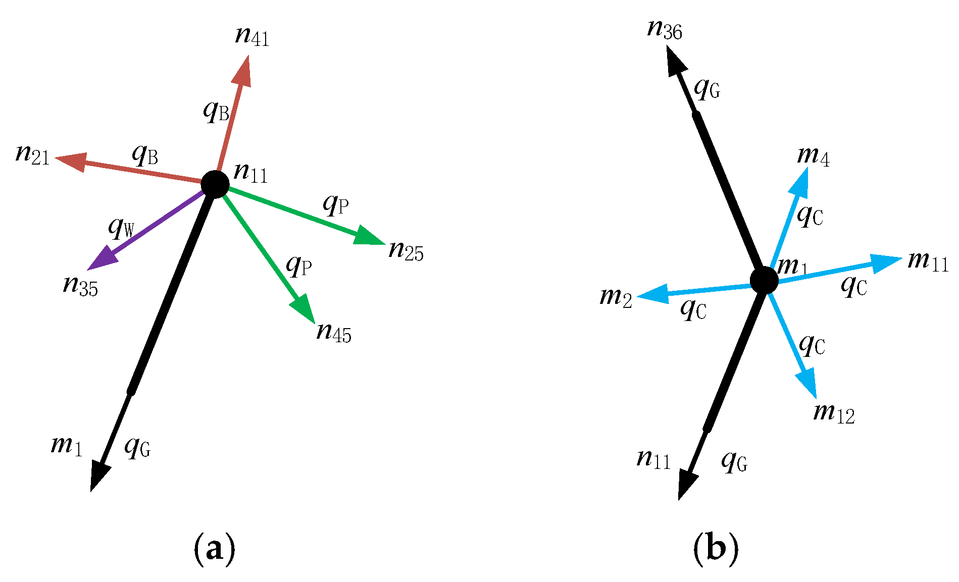
2.3.1. Establishment of Equilibrium Equations

The equilibrium equations of the structure are established to calculate the internal forces of the components and verify the self-equilibrium of the structure. The connections between bar components and cable components within the structure can be represented using a connection matrix denoted as $\mathit{C}\in {\mathbb{R}}^{f\times g}$. Each row of the matrix contains only two non-zero elements, 1 and −1, corresponding to the two nodes connected by a component, while all other elements of the matrix are zero. The connection matrix can be expressed as:

$$C_{\left(f, g\right)}=\left\{\begin{array}{l}1, \mathrm{n}\mathrm{o}\mathrm{d}\mathrm{e} g \mathrm{i}\mathrm{s} \mathrm{t}\mathrm{h}\mathrm{e} \mathrm{s}\mathrm{t}\mathrm{a}\mathrm{r}\mathrm{t}\mathrm{i}\mathrm{n}\mathrm{g} \mathrm{p}\mathrm{o}\mathrm{i}\mathrm{n}\mathrm{t} \mathrm{o}\mathrm{f} \mathrm{c}\mathrm{o}\mathrm{m}\mathrm{p}\mathrm{o}\mathrm{e}\mathrm{n}\mathrm{t} f\\ -1, \mathrm{n}\mathrm{o}\mathrm{d}\mathrm{e} g \mathrm{i}\mathrm{s} \mathrm{t}\mathrm{h}\mathrm{e} \mathrm{s}\mathrm{t}\mathrm{a}\mathrm{r}\mathrm{t}\mathrm{i}\mathrm{n}\mathrm{g} \mathrm{p}\mathrm{o}\mathrm{i}\mathrm{n}\mathrm{t} \mathrm{o}\mathrm{f} \mathrm{c}\mathrm{o}\mathrm{m}\mathrm{p}\mathrm{o}\mathrm{e}\mathrm{n}\mathrm{t} f\\ 0, \mathrm{o}\mathrm{t}\mathrm{h}\mathrm{e}\mathrm{r}\mathrm{w}\mathrm{i}\mathrm{s}\mathrm{e}\end{array}\right.$$

(10)

where f (f = 1, 2, …, 108) represents component number, and g (g = 1, 2, …, 36) represents the node number.

The coordinate vectors of nodes n_ij and m_k are be defined as x, y, z ($\in {\mathbb{R}}^g$). The vectors of the coordinate differences u_g, v_g, w_g between the two end nodes of each component are defined as u, v, w ($\in {\mathbb{R}}^f$).

$$\left\{\begin{array}{c}\mathit{u}=\mathit{C}\mathit{x}\\ \mathit{v}=\mathit{C}\mathit{y}\\ \mathit{w}=\mathit{C}\mathit{z}\end{array}\right.$$

(11)

Vector I ($\in {\mathbb{R}}^f$) is the collection of length vectors for each component. Diagonalizing the elements in the component vectors u, v, w and l yields the matrix form $\mathit{U},\mathit{V},\mathit{W},\mathit{L}\left(\in {\mathbb{R}}^{f\times f}\right)$ as shown below.

$$\left\{\begin{array}{c}\mathit{U}=diag\left(\mathit{u}\right)\\ \mathit{V}=diag\left(\mathit{v}\right)\\ \mathit{W}=diag\left(\mathit{w}\right)\\ \mathit{L}=diag\left(\mathit{l}\right)\end{array}\right.$$

(12)

According to the principle of virtual work, the necessary and sufficient condition for the structure to be in equilibrium is that the equilibrium equation of the structure, in the absence of external forces [33], can be expressed as:

$$\left\{\begin{array}{c}{\mathit{C}}^T\mathit{U}{\mathit{L}}^{-1}\mathit{s}={\mathit{D}}^x\mathit{s}=0\\ {\mathit{C}}^T\mathit{V}{\mathit{L}}^{-1}\mathit{s}={\mathit{D}}^y\mathit{s}=0\\ {\mathit{C}}^T\mathit{W}{\mathit{L}}^{-1}\mathit{s}={\mathit{D}}^z\mathit{s}=0\end{array}\right.$$

(13)

where $\mathit{s}(\in {\mathbb{R}}^f)$ is the vector of internal forces in the components of the structure.

Thus, when the structure is not subjected to external force, the matrix form of the equilibrium equation can be obtained:

$$\mathit{D}\mathit{s}=0$$

(14)

where the equilibrium matrix is $\mathit{D}\left(\in {\mathbb{R}}^{3g\times f}\right)=\left[\begin{array}{c}{\mathit{D}}^x\\ {\mathit{D}}^y\\ {\mathit{D}}^z\end{array}\right]$.

For the structure to have a non-zero solution for s in Equation (13) without external forces, the equilibrium matrix D must satisfy $\det \left(\mathit{D}\right)=0$. By solving the equilibrium Equation (13), the internal force vector s of the structural members can be obtained by:

$$\mathit{s}=k{\mathit{S}}_0$$

(15)

where k is a positive real number, and the basic solution system for member internal forces is ${\mathit{S}}_0=\left[\begin{array}{cccc}{s}_1& s_2& \dots & s_f\end{array}\right]$ (where f = 1, 2, …, 108).

The concept of force density is introduced: $q_f=s_f/l_f,q_f$ represents the force density, that is, the tension of the internal member per unit length; $s_f$ is the component tension, $l_f$ is the component length.

2.3.2. Self-Equilibrium Analysis

When verifying the self-equilibrium of the spherical tensegrity, the equilibrium of reference nodes is deduced based on the structure’s symmetry. The reference nodes n₁₁ and m₁ are as shown in Figure 3. The tension per unit length of the member, also referred to as the force density, q_f, which is introduced as:

$$q_f=s_f/l_f$$

(16)

where s_f is the member tension and l_f is the member length.

Let the force density of the six-bar members be q_G, the outer surface cables be q_B, the inner surface cables be q_C, the additional cables be q_P, and the diagonal cables be q_W. In the absence of external loads, the force density relationships at nodes n₁₁ and m₁ are as follows:

$$\begin{array}{c}{q}_B\left({\mathit{n}}_{21}-{\mathit{n}}_{11}\right)+q_B\left({\mathit{n}}_{41}-{\mathit{n}}_{11}\right)+q_P\left({\mathit{n}}_{25}-{\mathit{n}}_{11}\right)+\\ q_P\left({\mathit{n}}_{44}-{\mathit{n}}_{11}\right)+q_W\left({\mathit{n}}_{35}-{\mathit{n}}_{11}\right)-q_G\left({\mathit{m}}_1-{\mathit{n}}_{11}\right)=0\end{array}$$

(17)

$$\begin{array}{c}{q}_C\left({\mathit{m}}_2-{\mathit{m}}_1\right)+q_C\left({\mathit{m}}_4-{\mathit{m}}_1\right)+q_C\left({\mathit{m}}_{11}-{\mathit{m}}_1\right)+\\ q_C\left({\mathit{m}}_{12}-{\mathit{m}}_1\right)-q_G\left({n\mathit{n}}_{11}-{m\mathit{m}}_1\right)-q_G\left({\mathit{n}}_{36}-{\mathit{m}}_1\right)=0\end{array}$$

(18)

2.3.3. Self-Equilibrium Verification

In this structure, the external surface edge length b is set as 1 m, the unit spacing d is set as 0.7 m, and the range of unit heights is set as $h\in \left(0.35,0.85\right)$. The geometric model of the structure is first established. The nodal coordinates n₁₁ and m₁ are then calculated. These coordinates are subsequently substituted into Equation (12) to obtain the equilibrium matrix D of the structure. Finally, the internal force matrix s is solved using Equation (13), a feasible prestress mode is obtained. Due to the structure’s symmetry, the internal forces of the same type of components are equal. This applies to the outer surface cables, additional cables, inner surface cables, and diagonal cables. We set the force density of the bar members to −1 N/m whose positive and negative signs indicate tension and compression, respectively. The force density curves for various components at different unit heights are obtained by Equation (15), as shown in Figure 4.

2.4. Stability Determination of the Structure

Structural stability implies a state of self-equilibrium. However, a system in self-equilibrium is not necessarily stable. Therefore, an analysis on the stability of the given structure should be conducted. Initially, it is essential to classify its static and kinematic systems and solve for the independent mechanism displacement modes of the structure. Subsequently, the stability of the structure can be determined by examining the positive definiteness of its tangent stiffness matrix.

2.4.1. System Determination Based on Maxwell’s Criterion

According to Maxwell’s criterion, the structural system is determined by the relationship between the number of members, the number of nodes and the number of constraints in the hinged link system [35]. The number of self-stress modes ds and displacement modes dm of the structure can be calculated by:

$$\left\{\begin{array}{c}ds=f-r\\ dm=3\left(n_f-n_f^k\right)-r\end{array}\right.$$

(19)

where $n_f$ is the number of free nodes, $n_f^k$ is the number of constrained nodes, and r is the rank of the equilibrium matrix.

After calculation, for the spherical tensegrity structure, ds > 0 and dm > 0. The structure simultaneously possesses both mechanism displacement modes and self-stress modes. It belongs to type IV, a statically and kinematically indeterminate structure, as described in literature [36]. This structure can achieve a self-equilibrium state by introducing appropriate prestress.

2.4.2. Structural Stability Assessment

The stability of the structure is determined by assessing the positive definiteness of the tangent stiffness matrix. The structural stiffness matrix K is expressed as:

$$\mathit{K}={\mathit{K}}_E+{\mathit{K}}_G$$

(20)

where K_E is the elastic stiffness matrix, and K_G is the geometric stiffness matrix.

Assuming the elastic modulus of the structural components, the cross-sectional area, and the component length, the stiffness coefficient can be expressed and be used to establish the diagonal matrix ${\mathit{K}}_t\left(\in {\mathbb{R}}^{3g\times 3g}\right)$. The elastic stiffness matrix K_E can be calculated by:

$${\mathit{K}}_E=\mathit{D}{\mathit{K}}_t{\mathit{D}}^T$$

(21)

The geometric stiffness matrix represents the influence of prestress on overall stiffness and can be obtained by:

$${\mathit{K}}_G={\mathit{I}}_3\otimes \mathit{E}$$

(22)

where ${\mathit{I}}_3\left(\in {\mathbb{R}}^{3\times 3}\right)$ represents a third-order identity matrix, $\otimes$ denotes the tensor product, E is the force density matrix of components, $\mathit{E}={\mathit{C}}^T\mathit{Q}\mathit{C}$, and Q is the diagonal matrix for the component force densities.

The independent displacement modes of tensegrity structures can be directly deduced by the equilibrium matrix and the number of displacement modes dm [37], and an augmented matrix $\left.\mathit{D}\right|\mathit{I}$ is established. Multiple row transformations are performed on this matrix by Gaussian elimination, resulting in the matrix $\left.\bar{\mathit{D}}\right|\bar{\mathit{I}}$. The matrix corresponding to the bottom dm rows of $\bar{\mathit{I}}$ represents the independent mechanism displacement modes ${\mathit{d}}_{in}$ of the tensegrity structure. For tensegrity structures in self-equilibrium, stability can be assessed using the following sufficient condition [38]: When the structure type is kinematically indeterminate (i.e., $mm>0$), if the geometric stiffness matrix K_G is positive semi-definite and the matrix ${\mathit{d}}_{in}{\mathit{K}}_G{\mathit{d}}_{in}\in {\mathbb{R}}^{\left(3g-r-6\right)\times \left(3g-r-6\right)}$ is positive definite, the structure is stable. This condition allows for stability assessment without calculating specific values of the elastic stiffness matrix K_E, making it more applicable in practical engineering.

Taking the structural parameters in Section 2.3.3 as an example, MATLAB 2018 is employed to solve for the independent mechanism displacement modes ${\mathit{d}}_{in}$ and the matrix K_G from Equation (21). The specific eigenvalues of the geometric stiffness matrix K_G and ${\mathit{d}}_{in}{\mathit{K}}_G{\mathit{d}}_{in}$ are further calculated, as shown in Appendix A. From Appendix A, it can be observed that the minimum eigenvalue of matrix K_G is approximately zero (setting the eigenvalue threshold below 10⁻⁵ can be considered as zero), satisfying the positive semi-definiteness of the geometric stiffness matrix K_G. The minimum eigenvalues of matrix ${\mathit{d}}_{in}{\mathit{K}}_G{\mathit{d}}_{in}$ are all greater than zero, satisfying the positive definiteness of the matrix. Therefore, the structure achieves a stable state.

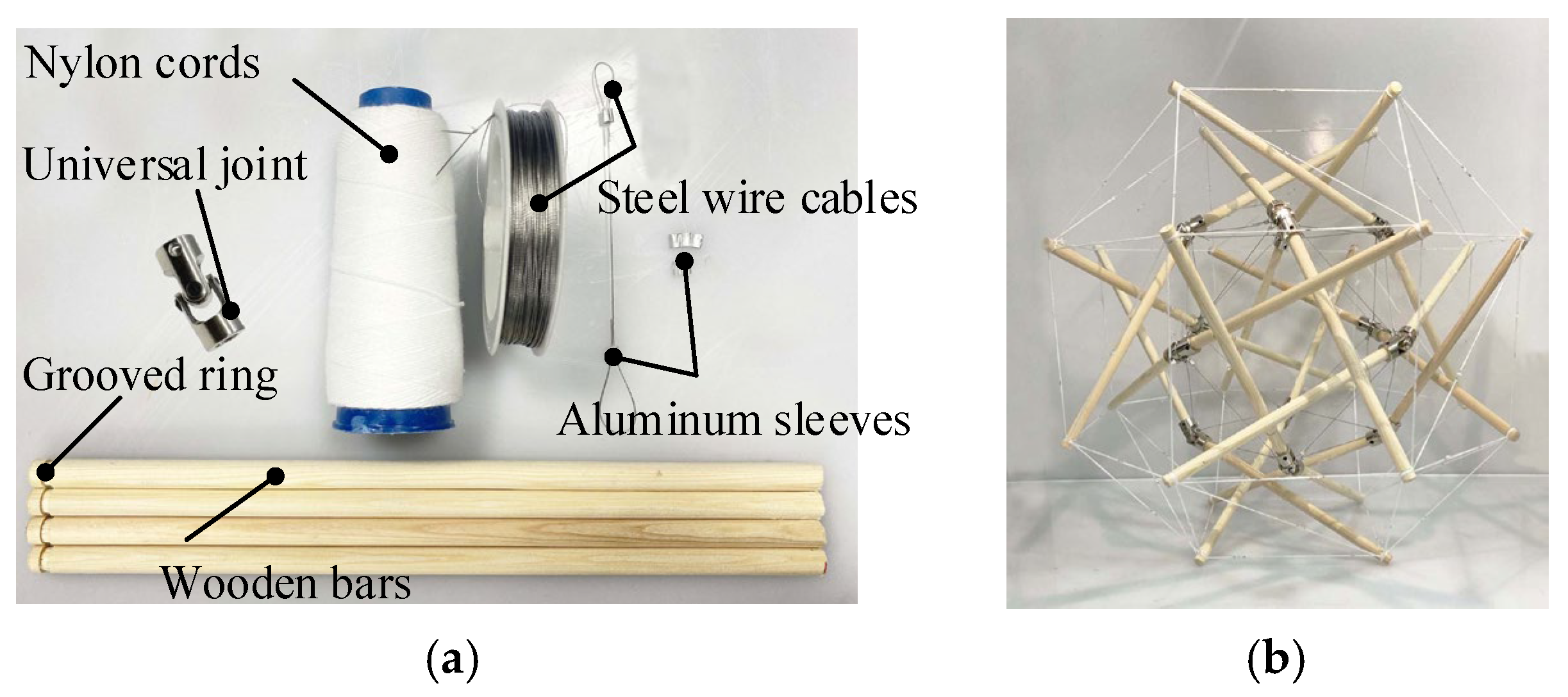
2.5. Construction of Physical Model

A physical model of the structure is constructed to verify its feasibility. When building the experimental model, a proportional scaling principle can be adopted. This ensures that internal forces are proportionally reduced while maintaining the positional relationships of the components, preserving the verification of self-equilibrium and stability of the original structure. Specifically, the geometric model from Section 2.3.3 is scaled down to one-eighth of its original size. This approach not only reduces material and time costs but also improves construction precision, providing a reference for future large-scale structure fabrication.

The bar components in the structure are replaced with 10 mm diameter wooden bars. One side of each bar features a grooved ring to facilitate cable connection, while the other side is fitted with a universal joint for class II assembly. The outer cable components are fixed to the wooden bars using 0.2 mm diameter white nylon cords tied in knots. For inner cable components, where knotting is impractical, 0.2 mm diameter soft steel wire cables are secured at the universal joint positions using aluminum sleeves. The experimental materials are shown in Figure 5a. Taking the parameters in Section 2.3.3 as an example, the physical model is established with a unit height of h = 0.5 m, the prestress of each component is the product of its length and force density. Components are connected according to the methods described in Section 2.1, resulting in the structural model. As illustrated in Figure 5b, the construction of this experimental model verifies the self-equilibrium and stability of the spherical tensegrity structure proposed in this paper, the shape error between the experimental model and the theoretical model mainly arises from the fact that the length of the same type of cable cannot be completely consistent.

3. Static Characteristic Analysis

Tensegrity belongs to the space truss structure with small strain and large deformation. Considering the complicated connection of cable-strut unit and its geometric nonlinear characteristics, the finite element model is established by programming in APDL of ANSYS 19.2, and the influencing factors of compressive stiffness of the structure are analyzed in the category of statics.

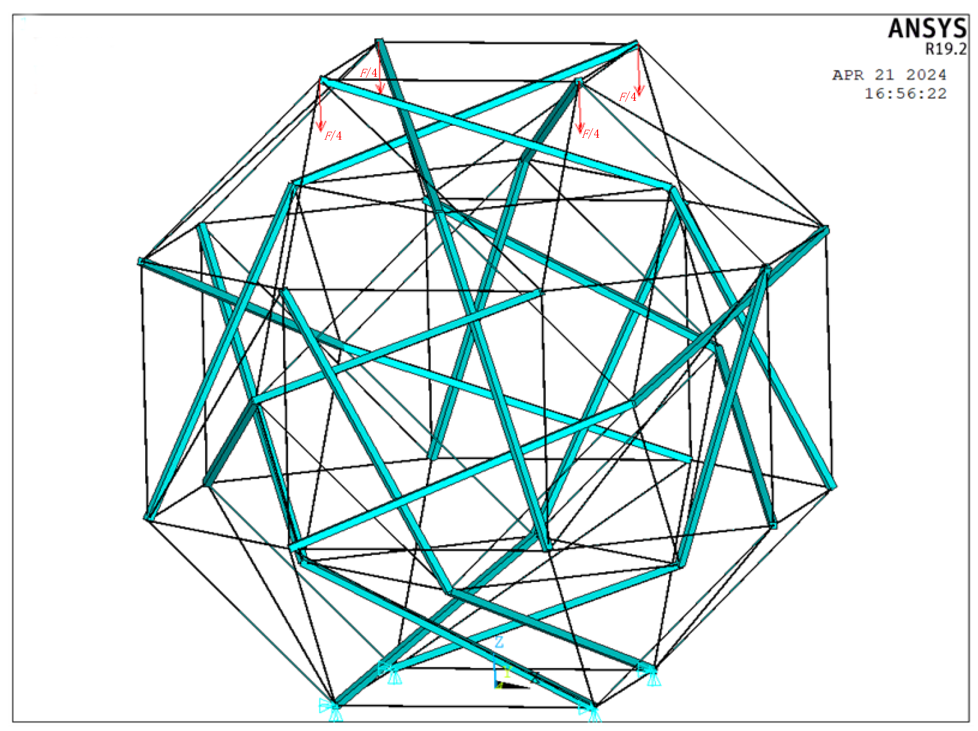
3.1. Establishment of Finite Element Model

In ANSYS APDL, Link180 elements were selected to model both the compressive bars and tensile cables, with initial pre-strain applied to simulate the prestressed state. Accounting for geometric nonlinearity under external loading conditions, the large deformation option was enabled to systematically analyze the effects of member cross-sectional area and cable prestress on the structural compressive stiffness.

Taking the structural parameters in Section 2.3.3 as an example, a simulation model is established with a unit height of h = 0.5 m. The parameters of the structure are detailed in

Table 2. Finite element simulation parameters.

Component Class	Bars	Cables
Element type	Link180	Link180
Element attribute	Compression-only	Tension-only
Cross-sectional area/mm2	706.86	40.72
Elasticity modulus/Gpa	206	185
Poisson’s ratio	0.3	0.3
Density/kg·m−3	7850	7850
Thermal expansivity/K−1	10−5	10−5

. The model contains 36 nodes and 108 elements. The bottom node n₁₁ is constrained in the x, y, z directions, other nodes n₂₁, n₃₁, and n₄₁ are constrained in the z direction. External loads $F/4$ are applied to the top nodes n₁₂, n₂₂, n₃₂, and n₄₂ along the negative z-axis direction. The finite element model of the designed spherical structures is shown in Figure 6. The displacement of the top nodes along negative z-direction is denoted by $U$. The compressive stiffness of the structure can be calculated by:

$$K_U=F/U$$

(23)

3.2. Finite Element Simulation Analysis

Through the study of the stiffness matrix, it is found that after the configuration of the tensegrity is determined, the length and position relationship of the components are also limited, but the elastic stiffness and geometric stiffness can be changed by adjusting the cross-sectional area of the components and the prestress of the components, so as to further adjust the stiffness of the structure. Therefore, this section will analyze the influence of cross-sectional area of different bar members and different prestress levels on structural stiffness through finite element simulation software.

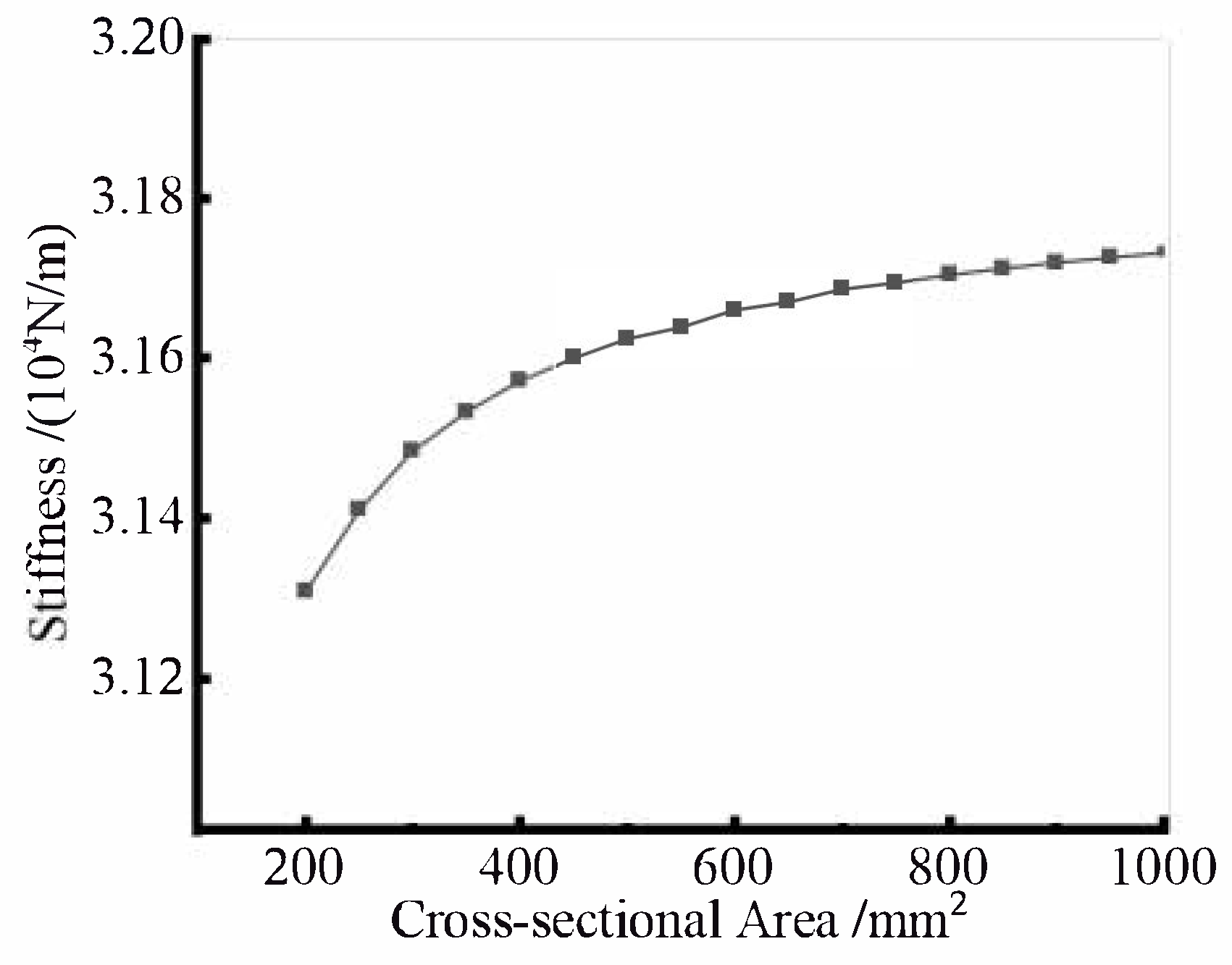
3.2.1. Analysis of the Influence of Cross-Sectional Area of Bar Members on Stiffness

When k = 400, the set of $\epsilon \in {\mathbb{R}}^f$ for all components in the structure is obtained from Equation (14). A prestress of the structure 1.25ε, and an external load of 1000 N are applied to the spherical structure.

As shown in Figure 7, it is observed that the compressive stiffness of the spherical structure increases with the cross-sectional area of bar components. The structure exhibits a rapid increase in compressive stiffness when the cross-sectional area is between 200–600 mm². However, when the cross-sectional area exceeds 600 mm², the rate of increase in compressive stiffness begins to slow down. The compressive stiffness of the spherical structure is 7.118 × 10⁴ N/m.

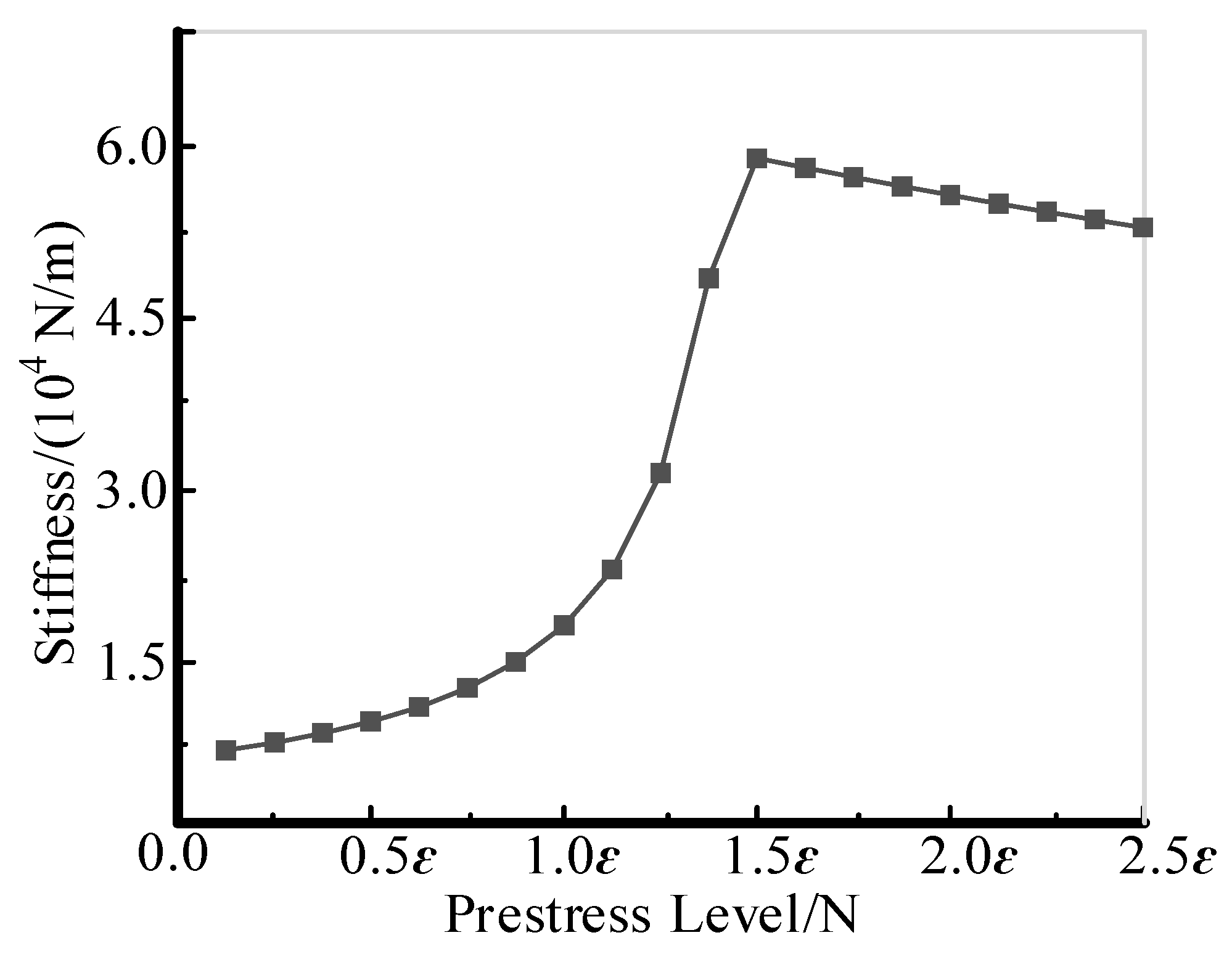
3.2.2. Analysis of the Influence of Prestress on Stiffness

Based on the above analysis results, when the component cross-sectional area is set to 300 mm² and a 1000 N external load is applied, the relationship between compressive stiffness and prestress level for the spherical structure is shown in Figure 8. It indicates that, as the prestress level increases, with the premise of keeping the size of each component unchanged, the compressive stiffness of the spherical structure first increases and then decreases. The increase in compressive stiffness is gradual when the prestress level is in the range of 0–1.0ε. The rate of increase reaches its maximum between 1.0ε and 1.5ε. The compressive stiffness peaks at 5.897 × 10⁴ N/m near a prestress level of 1.5ε. Beyond 1.5ε, the compressive stiffness begins to decrease steadily, as the axial force at both ends of the compression bar exceeds its critical load. This phenomenon indicates that the compressive stiffness of the spherical structure is sensitive to prestress. Therefore, the prestress level is crucial in structural design and performance optimization.

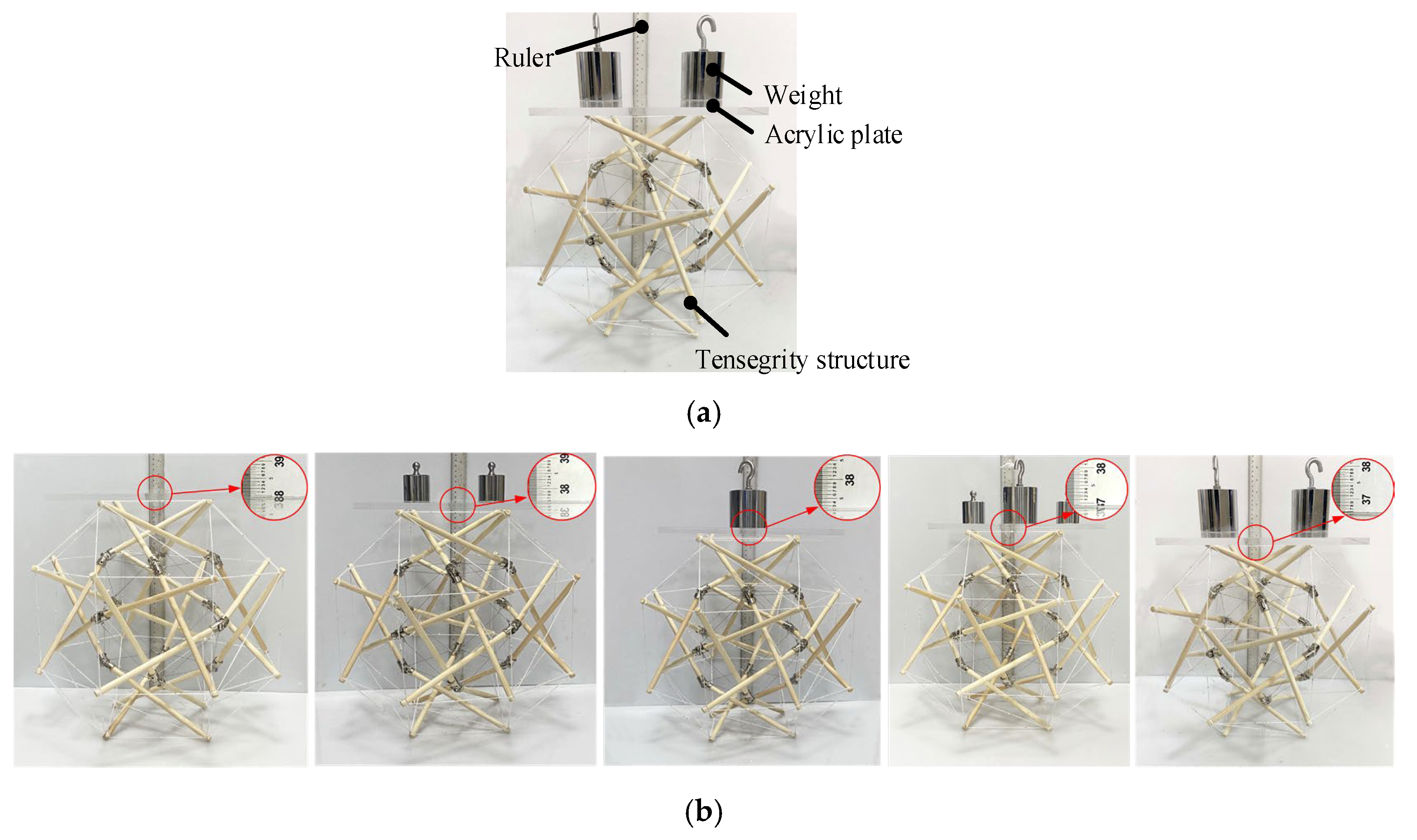
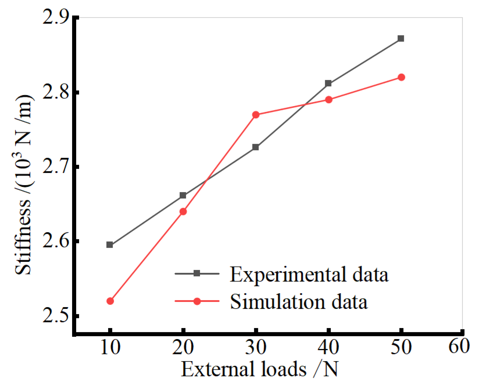
3.3. Stiffness Experiment

Based on the parameters in Table 2, a scaled prototype model, whose size is one-tenth of the geometric model, is conducted to verify the accuracy of the finite element simulation results. The physical model is placed on the ground, and a vertical downward load is applied through weights and an acrylic plate on top of the structure. A ruler is used to measure the height changes of the nodes on the top surface of the structure. The experimental setup is shown in Figure 9a. Stiffness experiments are conducted by applying external loads of 10 N, 20 N, 30 N, 40 N, and 50 N on top of the structure, as shown in Figure 9b.

The height changes of the nodes are recorded both when the structure is under compression from different external loads and after the loads are removed. The experimental stiffness data is calculated by Equation (23). Simultaneously, referring to the simulation process in Section 3.2, a stiffness simulation is performed again using the material and dimensional parameters of the physical model in this section. The simulation stiffness data for the physical model is obtained. A comparison between the experimental data and simulation data is shown in Figure 10. The maximum discrepancy between simulation and experimental results is merely 2.778%, with consistent variation trends observed in both cases, demonstrating the stiffness variation under external loading conditions.

4. Analysis of Cushioning Performance Based on Collision Simulation

The spherical tensegrity structure is often used as a cushioning mechanism for space exploration landing devices due to its excellent cushioning performance. Based on spatial limitation, only the most ideal scenario where the four bottom nodes collide with the plane simultaneously is studied here. ADAMS 2018 software is employed to conduct collision simulations on the two structures, and the factors affecting their cushioning performance are be analyzed. Subsequently, the cushioning performance of the structure are verified through a physical prototype testing.

4.1. Dynamic Collision Simulation

In the collision simulation, rigid bodies are used to model the bar components based on the inertial coordinate system O₁ introduced in Section 2.2 and the connection relationships between nodes, while springs are used to simulate cable components. By setting the spring tension and compression stiffness coefficients, damping coefficients, and spring preload forces, the structure achieves a self-balanced stable state in the absence of external forces. The collision forces between two components are calculated by the IMPACT function in ADAMS software, which equivalently models the contact between the structure and the ground as a spring-damper model. The specific collision simulation parameters are shown in

Table 3. Collision simulation parameters.

Simulation Parameters	Parameter Values
Gravity/N·kg−1	9.8
Landing height/m	8
Elastic modulus of the bar/Gpa	206
Density of the bar/kg·m−3	7850
Cross-sectional area of the bar/mm2	706.86
Poisson’s ratio of the bar	0.3
Elasticity modulus of the cable/Gpa	185
Density of the cable/kg·m−3	7850
Cross-sectional area of the cable/mm2	40.72
Poisson’s ratio of the cable	0.3
Stiffness of the contact surface/N·m−1	104
Damping coefficient of the contact surface/N·s·m−1	10
Invasion depth/mm	0.1

.

Set the gravitational acceleration to the -y direction, the spherical structure is dropped from 0 to −8 m with an initial velocity of zero and undergoes free motion. The collision process between the structure and the ground is simulated and illustrated in Figure 11, where blue components represent spring cables, internal red rigid bodies represent bar components, and the gray bottom layer represents the ground. During the collision with the ground, the maximum height of centroid of the structure reflects its cushioning capacity, while changes in kinetic energy and spring potential energy reveal its energy absorption characteristics. The influence of different structural parameters on the cushioning performance during the landing process is be analyzed.

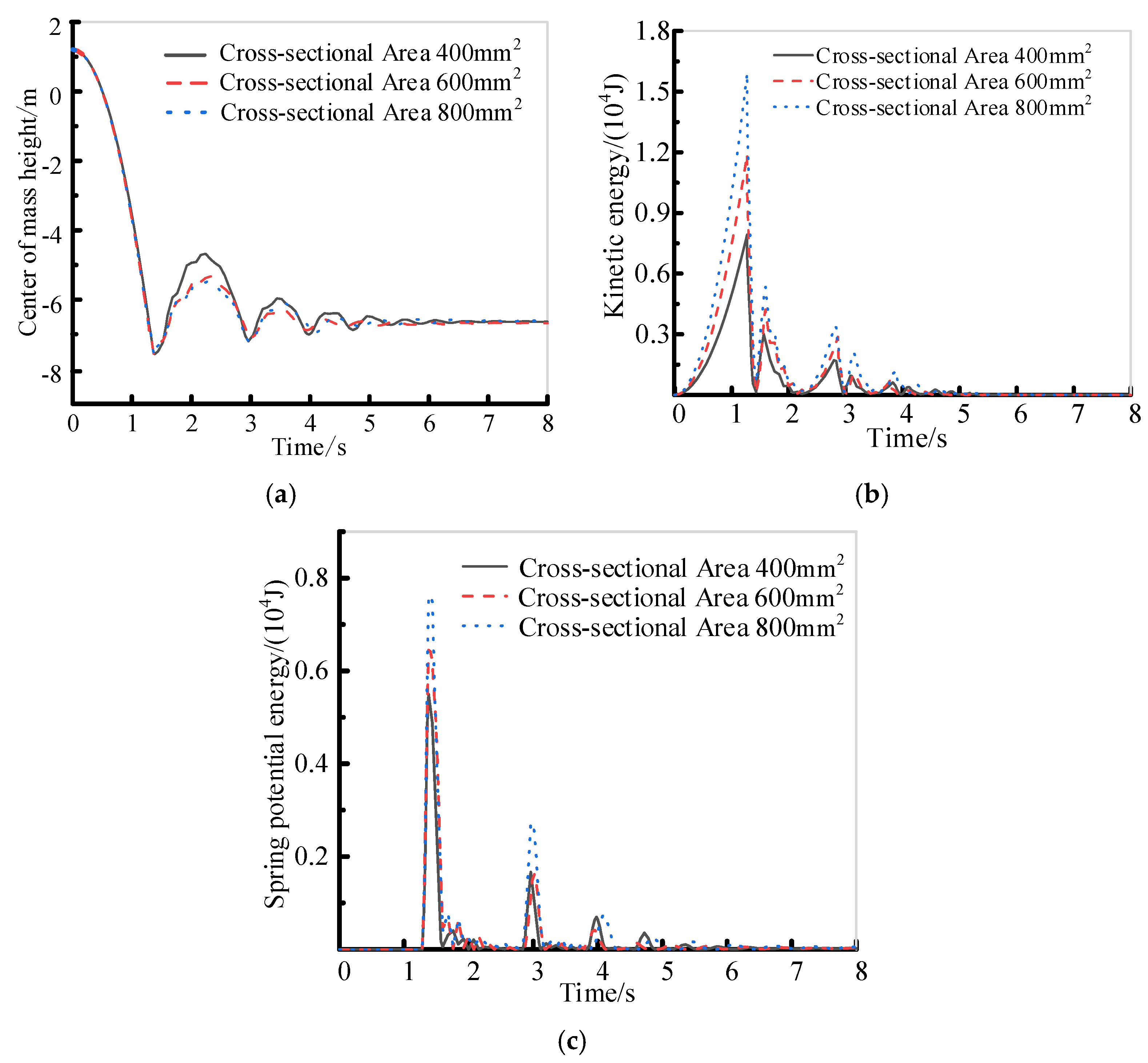
4.2. Analysis of the Impact of Bar Component Cross-Sectional Area on Cushioning Performance

To investigate the influence of the cross-sectional area of bar components on the cushioning performance of the spherical tensegrity structure, a selected structure with a prestress of 1.5ε, spring tension and compression stiffness coefficient of 10⁴ N/m, and spring damping coefficient of 100 N·s/m is studied. Collision simulations are conducted with bar component cross-sectional areas of 400 mm², 600 mm², and 800 mm². The resulting curves of the height of the centroid of the structure and energy changes over time are shown in Figure 12.

In Figure 12, it can be observed that both structures initially contact with the ground at 1.28 s. Subsequently they reach their highest position at 2.3 s, after which a second collision with the ground occurs at around 3 s. Figure 12a demonstrates that when the bar component’s cross−sectional area is increased from 400 mm² to 600 mm², the maximum rebound height of the structure’s center of mass decreases. However, when the cross−sectional area is further increased to 800 mm², the maximum rebound height remains almost unchanged. This phenomenon occurs because a moderate increase in the bar component’s cross−sectional area enhances the structure’s cushioning performance, resulting in a lower rebound height. However, when the increase in cross−sectional area exceeds a certain threshold, the additional cushioning effect is offset by the increased weight of the structure, leading to limited changes in the rebound height. Figure 12b,c show that the structure’s mass also increases with the bar component’s cross−sectional area, resulting in higher maximum kinetic energy and spring potential energy. The structure reaches its maximum kinetic energy at 1.28 s, while the spring potential energy peaks at 1.41 s. Based on these observations, it can be concluded that moderately increasing the cross−sectional area of the bar components can improve the structure’s cushioning capacity.

4.3. Analysis of the Impact of Spring Prestress on Cushioning Performance

To investigate the influence of spring prestress on the cushioning performance of the spherical tensegrity structure, a spherical structure with bar component cross−sectional area of 800 mm², a spring tension and compression stiffness coefficient of 10⁴ N/m, and a spring damping coefficient of 100 N·s/m is established. Collision simulations are conducted with cable prestress values of 1.0ε, 1.25ε, and 1.5ε, the performance of the structures are shown in Figure 13.

Figure 13a shows that the height of the centroid of the structure is around −4.3 m with a prestress of 1.0ε. When the prestress is increased to 1.25ε and 1.5ε, the structure exhibit maximum center of mass heights of approximately −4.8 m. This indicates that as the prestress level in the structure increases, the maximum rebound height of the spherical structure first decreases and then stabilizes. Therefore, increasing the prestress level improves cushioning performance, but the improvement is limited.

Figure 13b,c show that after collision, the potential energy stored in the springs of structures with prestress values of 1.0ε and 1.25ε is significantly lower than that of the structure with 2.0ε prestress. This indicates that while maintaining relatively constant spring potential energy changes, moderately increasing prestress can enhance the structure’s cushioning performance. However, excessive prestress may cause collision energy to be converted into spring potential energy, preventing the structure from dissipating kinetic energy through its inherent cushioning characteristics.

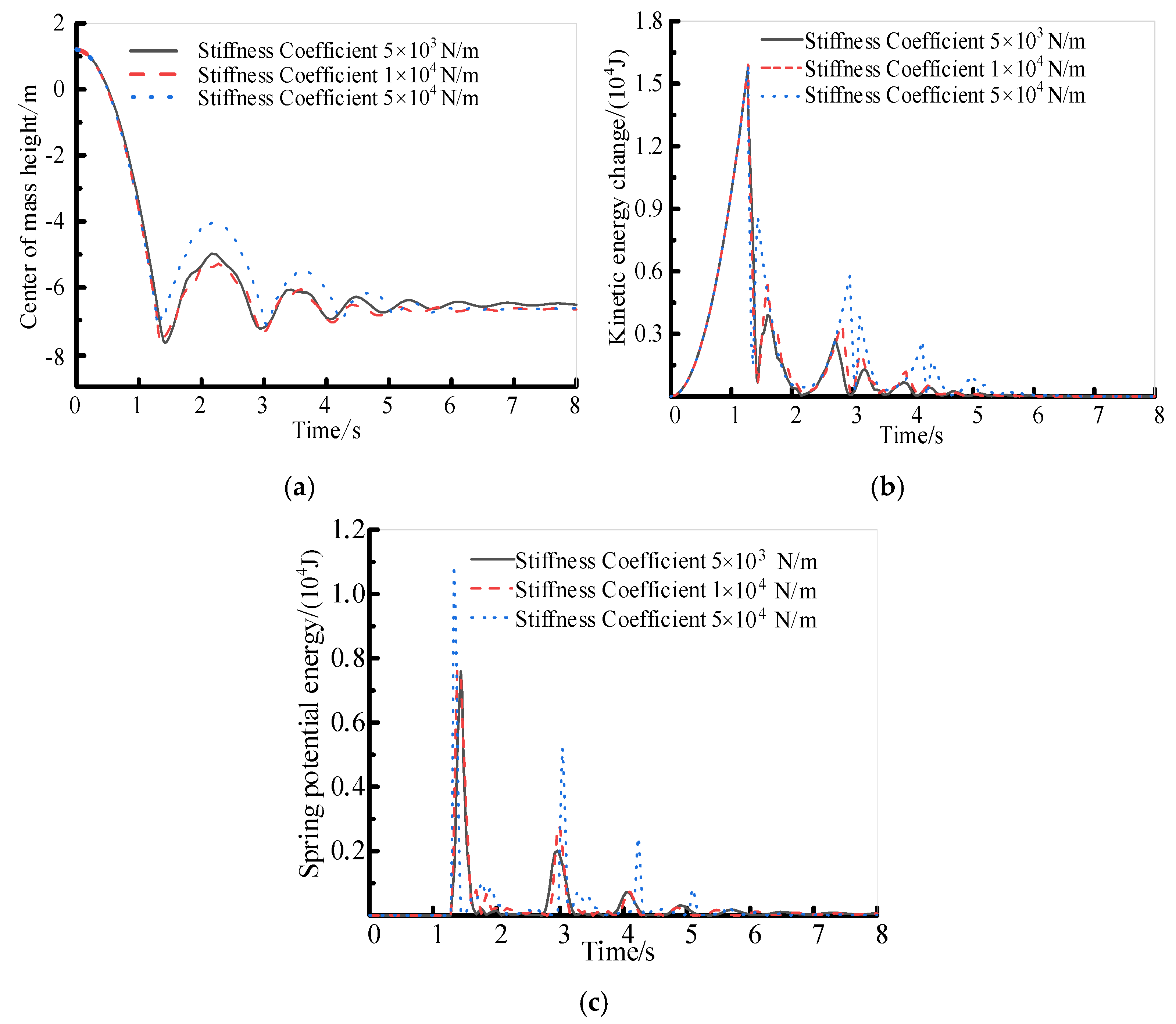
4.4. Analysis of the Impact of Spring Tension and Compression Stiffness Coefficient on Cushioning Performance

To investigate the influence of the spring tension and compression stiffness coefficient on the cushioning performance of the spherical tensegrity structure, a spherical structure with a bar component cross−sectional area of 800 mm², a prestress of 1.5ε, and a spring damping coefficient of 100 N·s/m is studied. Collision simulations were conducted with spring tension and compression stiffness coefficients of 5 × 10³ N/m, 10⁴ N/m, and 5 × 10⁴ N/m, the resulting curves of the structure’s center of mass height and energy changes over time are shown in Figure 14.

In Figure 14, When the stiffness coefficient is 5 × 10³ N/m, the maximum bounce height is −5 m, and the maximum spring potential energy is 0.75 × 10⁴ J. When the stiffness coefficient is 10⁴ N/m, the maximum bounce height is −4.8 m, and the maximum spring potential energy is 0.76 × 10⁴ J. When the stiffness coefficient is 5 × 10⁴ N/m, the maximum bounce height is −3.8 m, and the maximum spring potential energy is 1.08 × 10⁴ J. It can be observed that as the spring stiffness increases, both the structure’s maximum rebound height and maximum spring potential energy increase significantly. The structure “harder” occurs the increase in spring stiffness, resulting in a larger proportion of kinetic energy being converted into elastic potential energy of the springs rather than being dissipated through deformation or other forms. This energy conversion mechanism reduces the possibility of energy dissipation through the structure’s inherent cushioning characteristics, thereby relatively weakening its cushioning capacity. Therefore, precise control of the spring stiffness in the spherical structure is necessary. This ensures that while improving energy absorption efficiency, the overall cushioning performance is not reduced due to excessive structural rigidity.

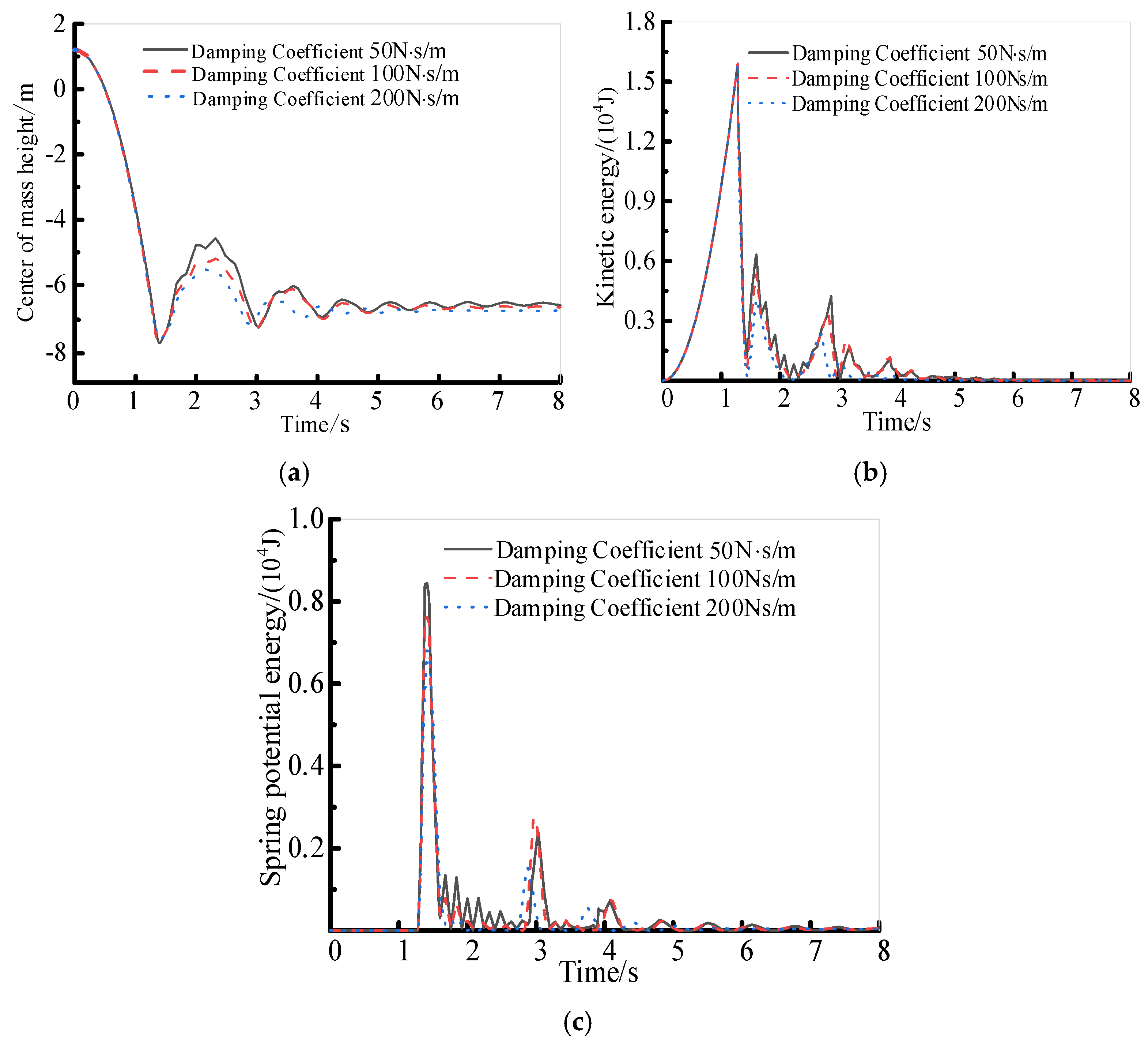
4.5. Analysis of the Impact of Spring Damping Coefficient on Cushioning Performance

To investigate the influence of the spring damping coefficient on the cushioning performance of the spherical tensegrity structure, a spherical structure with bar component cross−sectional area of 800 mm², prestress of 1.5ε, and spring stiffness coefficient of 10⁴ N/m is studied. Collision simulations are conducted with spring damping coefficients of 50 N·s/m, 100 N·s/m, and 200 N·s/m. The resulting curves of the structure’s center of mass height and energy changes over time are shown in Figure 15.

In Figure 15, it can be observed that as the spring damping coefficient gradually increases, the maximum rebound height of the structure after collision consistently decreases. The lowest heights for the three structures decrease to −4.2 m, −6.0 m, and −5.8 m respectively. Simultaneously, the spring potential energy in the structure also shows a slight decline during this process. At a damping coefficient of 200 N·s/m, the maximum rebound height is −5.3 m, and the maximum spring potential energy is 0.68 × 10⁴ J. This phenomenon occurs because the increase in damping coefficient significantly enhances the vibration suppression performance of the structure. This leads to more rapid and effective energy dissipation during the collision process, thereby substantially improving the overall cushioning performance of the structure. In conclusion, reasonable adjustment of the spring damping coefficient in the structure can effectively optimize the energy management and dispersion mechanism after collision. This not only reduces the maximum rebound height of the structure but also decreases the potential energy stored in the springs, thereby improving the safety and reliability of the structure during the collision process.

4.6. Collision Experiment

This section describes a landing collision experiment designed to evaluate the cushioning performance of the spherical structure proposed in this study. To provide a clear and intuitive assessment of the cushioning effects of structure, common and fragile chicken eggs are used as the protected payload in experiment. The integrity of the eggs after landing will serve as an indicator of effective payload protection.

The experimental model with parameters identical to those in Section 2.5 is utilized for the collision experiment. One end of the cable is connected to the structure’s nodes, while the other end is attached to the protected payload, securing it at the center of the structure, as depicted in Figure 16a. After ensuring the experimental area is clear of personnel, this structure is released to undergo free−fall motion with zero initial velocity, as illustrated in Figure 16b.

During the experiment, the landing height of the structure is incrementally increased until failure occurs, defined as either internal payload breakage or structural damage. Experimental data is collected on the maximum rebound height after the first collision at various landing heights, as well as whether the structure fails at each height. Additionally, following the collision simulation process in Section 4.1, simulation data is obtained for the maximum rebound height and the maximum internal spring force at different heights. The experimental and simulation data are compared in

Table 4. Collision experiment data for spherical structures.

HL/m	Experimental		Simulation		The Error of HMR
	Whether Failed	HMR/m	FMS/N	HMR/m
2	No	0.07	13.31	0.10	30.00%
3	No	0.17	17.07	0.25	32.00%
4	No	0.21	23.57	0.34	38.24%
5	No	0.40	36.05	0.49	18.37%
6	Yes	——	50.24	——	——

, where HL represents landing height, HMR is the maximum rebound height, FMS is the maximum spring internal force. Table 4 demonstrates that the maximum rebound height increasing as the landing height rises, and the structures fail at heights of 6 m, this spherical tensegrity structures exhibit great cushioning effect.

5. Conclusions

(1)

Based on the concept of circumferential assembling in tensegrity structures, a spherical tensegrity structure was designed by connecting six four−bar truncated pyramid units using type II assembly. Based on the established geometric model of the structure, the internal forces of the components were calculated, which verify the self−balance of the structure. The stability of the structure was confirmed through analysis of the positive definiteness of its tangent stiffness matrix. Finally, the feasibility of the structure was validated through a physical experiment.

(2)

The finite element model was established in ANSYS APDL, and key factors affecting structural compressive stiffness were analyzed through finite element simulation. Results indicate that the structure’s compressive stiffness increases with larger bar cross−sectional areas, though the rate of increase diminishes when the area exceeds 600 mm². Additionally, cable prestress significantly influences compressive stiffness. As prestress level increases, compressive stiffness initially rises, then declines, peaking at a prestress level of 1.5ε.

(3)

The collision simulations demonstrated that the structure’s cushioning performance is related to multiple structural parameters. A moderate increase in the bar component’s cross−sectional area can enhance the structure’s cushioning performance. Then the effect will be weakened by the offsetting effect of the increase in structural mass. Increasing the cable component prestress can improve the structure’s cushioning performance, but excessive prestress will lead to the instability of the bars. In addition, selecting an appropriate spring stiffness can improve the structure’s energy absorption efficiency without making it overly rigid, which would reduce its overall cushioning performance. Adjusting the spring damping coefficient in the structure can effectively optimize the energy management and dispersion mechanism after collision, enhancing the safety and reliability of the structure during the collision process.

References

1. Lu, J.; Dong, X.; Zhao, X.; Wu, X.; Shu, G. Form−finding analysis for a new type of cable–strut tensile structures generated by semi−regular tensegrity. Adv. Struct. Eng. 2017, 20, 772–783. [Google Scholar] [CrossRef]
2. Wang, X.; Ling, Z.; Qiu, C.; Song, Z.; Kang, R. A four−prism tensegrity robot using a rolling gait for locomotion. Mech. Mach. Theory 2022, 172, 104828. [Google Scholar] [CrossRef]
3. Gómez-Jauregui, V.; Carrillo-Rodríguez, Á.; Manchado, C.; Lastra-González, P. Tensegrity Applications to Architecture, Engineering and Robotics: A Review. Appl. Sci. 2023, 13, 8669. [Google Scholar] [CrossRef]
4. Da Silva, A.R.; de Souza, L.C.G.; Schäfer, B. Joint dynamics modeling and parameter identification for space robot applications. Math. Probl. Eng. 2007, 2007, 012361. [Google Scholar] [CrossRef]
5. Agogino, A.K.; SunSpiral, V.; Atkinson, D. Super Ball Bot−Structures for Planetary Landing and Exploration; Technical Report; NASA: Washington, DC, USA, 2018.
6. Zhang, P.; Zhou, J.; Chen, J. Form−finding of complex tensegrity structures using constrained optimization method. Compos. Struct. 2021, 268, 113971. [Google Scholar] [CrossRef]
7. Liu, Y.; Bi, Q.; Yue, X.; Wu, J.; Yang, B.; Li, Y. A review on tensegrity structures−based robots. Mech. Mach. Theory 2022, 168, 104571. [Google Scholar] [CrossRef]
8. Friesen, J.M.; Glick, P.; Fanton, M.; Manovi, P.; Xydes, A.; Bewley, T.; Sunspiral, V. The second generation prototype of a Duct Climbing Tensegrity robot, DuCTTv2. In Proceedings of the 2016 IEEE International Conference on Robotics and Automation (ICRA), Stockholm, Sweden, 16–21 May 2016; IEEE: Piscataway, NJ, USA, 2016; pp. 2123–2128. [Google Scholar]
9. Booth, J.W.; Cyr-Choiniere, O.; Case, J.C.; Shah, D.; Yuen, M.C.; Kramer-Bottiglio, R. Surface actuation and sensing of a tensegrity structure using robotic skins. Soft Robot. 2021, 8, 531–541. [Google Scholar] [CrossRef] [PubMed]
10. He, Z.; Han, L.; Zhang, X.; Zhang, L. Study on Folding and Rolling Performance of a Six−strut Spherical Tensegrity. Aerosp. Shanghai 2022, 39, 59–65. [Google Scholar]
11. Ma, S.; Chen, M.; Skelton, R.E. Tensegrity system dynamics based on finite element method. Compos. Struct. 2022, 280, 114838. [Google Scholar] [CrossRef]
12. Goyal, R.; Peraza Hernandez, E.A.; Majji, M.; Skelton, R.E. Design of Tensegrity Structures with Static and Dynamic Modal Requirements. In Earth and Space 2021; American Society of Civil Engineers: Reston, VA, USA, 2021. [Google Scholar]
13. Chen, M.; Goyal, R.; Majji, M.; Skelton, R.E. Deployable Tensegrity Lunar Tower. In Earth and Space; American Society of Civil Engineers: Reston, VA, USA, 2021; pp. 1079–1092. [Google Scholar]
14. Saha, D.; Goyal, R.; Skelton, R.E. Tensegrity Lander Architectures for Planetary Explorations. In Earth and Space; American Society of Civil Engineers: Reston, VA, USA, 2021; pp. 1251–1262. [Google Scholar]
15. Shibata, M.; Saijyo, F.; Hirai, S. Crawling by body deformation of tensegrity structure robots. In Proceedings of the 2009 IEEE International Conference on Robotics and Automation, Kobe, Japan, 12–17 May 2009; IEEE: Piscataway, NJ, USA, 2009; pp. 4375–4380. [Google Scholar]
16. Koizumi, Y.; Shibata, M.; Hirai, S. Rolling tensegrity driven by pneumatic soft actuators. In Proceedings of the 2012 IEEE International Conference on Robotics and Automation, Saint Paul, MN, USA, 14–18 May 2012; IEEE: Piscataway, NJ, USA, 2012; pp. 1988–1993. [Google Scholar]
17. Iscen, A.; Agogino, A.; SunSpiral, V.; Tumer, K. Learning to control complex tensegrity robots. In Proceedings of the 2013 International Conference on Autonomous Agents and Multi−Agent Systems, Saint Paul, MN, USA, 6–10 May 2013; pp. 1193–1194. [Google Scholar]
18. Hirai, S.; Imuta, R. Dynamic simulation of six−strut tensegrity robot rolling. In Proceedings of the 2012 IEEE International Conference on Robotics and Biomimetics (ROBIO), Guangzhou, China, 11–14 December 2012; IEEE: Piscataway, NJ, USA, 2012; pp. 198–204. [Google Scholar]
19. Sabelhaus, A.P.; Bruce, J.; Caluwaerts, K.; Manovi, P.; Firoozi, R.F.; Dobi, S.; Agogino, A.M.; SunSpiral, V. System design and locomotion of SUPERball, an untethered tensegrity robot. In Proceedings of the 2015 IEEE International Conference on Robotics and Automation (ICRA), Seattle, WA, USA, 26–30 May 2015; IEEE: Piscataway, NJ, USA, 2015; pp. 2867–2873. [Google Scholar]
20. Burms, J.; Caluwaerts, K.; Dambre, J. Online unsupervised terrain classification for a compliant tensegrity robot using a mixture of echo state networks. In Proceedings of the 2015 IEEE International Conference on Robotics and Automation (ICRA), Seattle, WA, USA, 26–30 May 2015; IEEE: Piscataway, NJ, USA, 2015; pp. 4252–4257. [Google Scholar]
21. Vespignani, M.; Friesen, J.M.; SunSpiral, V.; Bruce, J. Design of SUPERball v2, a compliant tensegrity robot for absorbing large impacts. In Proceedings of the 2018 IEEE/RSJ International Conference on Intelligent Robots and Systems (IROS), Madrid, Spain, 1–5 October 2018; IEEE: Piscataway, NJ, USA, 2018; pp. 2865–2871. [Google Scholar]
22. Bohm, V.; Kaufhold, T.; Schale, F.; Zimmermann, K. Spherical Mobile Robot Based on a Tensegrity Structure with Curved Compressed Members. In Proceedings of the 2016 IEEE International Conference on Advanced Intelligent Mechatronics (AIM), Banff, AB, Canada, 12–15 July 2016; pp. 1509–1514. [Google Scholar]
23. Bohm, V.; Kaufhold, T.; Zeidis, I.; Zimmermann, K. Dynamic analysis of a spherical mobile robot based on a tensegrity structure with two curved compressed members. Arch. Appl. Mech. 2017, 87, 853–864. [Google Scholar] [CrossRef]
24. Kim, K.; Moon, D.; Bin, J.Y.; Agogino, A.M. Design of a spherical tensegrity robot for dynamic locomotion. In Proceedings of the 2017 IEEE/RSJ International Conference on Intelligent Robots and Systems (IROS), Vancouver, BC, Canada, 24–28 September 2017; IEEE: Piscataway, NJ, USA, 2017; pp. 450–455. [Google Scholar]
25. Zhang, J.; Ohsaki, M. Self−equilibrium and stability of regular truncated tetrahedral tensegrity structures. J. Mech. Phys. Solids 2012, 60, 1757–1770. [Google Scholar] [CrossRef]
26. Zhang, J.; Ohsaki, M.; Tsuura, F. Self−equilibrium and super−stability of truncated hexahedral and octahedral tensegrity structures. Int. J. Solids Struct. 2019, 161, 182–192. [Google Scholar] [CrossRef]
27. Kim, K.; Chen, L.H.; Cera, B.; Daly, M.; Zhu, E.; Despois, J.; Agogino, A.K.; SunSpiral, V.; Agogino, A.M. Hopping and rolling locomotion with spherical tensegrity robots. In Proceedings of the 2016 IEEE/RSJ International Conference on Intelligent Robots and Systems (IROS), Daejeon, Republic of Korea, 9–14 October 2016; IEEE: Piscataway, NJ, USA, 2016; pp. 4369–4376. [Google Scholar]
28. Chen, L.H.; Kim, K.; Tang, E.; Li, K.; House, R.; Zhu, E.L.; Fountain, K.; Agogino, A.M.; Agogino, A.; Sunspiral, V.; et al. Soft spherical tensegrity robot design using rod−centered actuation and control. J. Mech. Robot. 2017, 9, 025001. [Google Scholar] [CrossRef]
29. Schroeder, K.K. A Comprehensive Entry, Descent, Landing, and Locomotion (EDLL) Vehicle for Planetary Exploration. Ph.D. Thesis, Virginia Tech, Blacksburg, VA, USA, 2017. [Google Scholar]
30. Gebara, C.A.; Carpenter, K.C.; Woodmansee, A. Tensegrity Ocean world landers. In Proceedings of the AIAA Scitech 2019 Forum, San Diego, CA, USA, 7–11 January 2019; p. 0868. [Google Scholar]
31. Zhao, L.; Peraza Hernandez, E.A. Tensegrity structures for impact energy absorption and dissipation in planetary landers. In Earth and Space 2021; American Society of Civil Engineers: Reston, VA, USA, 2021; pp. 908–919. [Google Scholar]
32. Wu, L.; de Andrade, M.J.; Brahme, T.; Tadesse, Y.; Baughman, R.H. A reconfigurable robot with tensegrity structure using nylon artificial muscle. Act. Passiv. Smart Struct. Integr. Syst. 2016, 2016, 9799. [Google Scholar]
33. Zhang, J.Y.; Ohsaki, M. Tensegrity Structures: Form, Stability, and Symmetry; Springer: Tokyo, Japan, 2015. [Google Scholar]
34. Mark, W. Spong. In Robot Dynamics and Control; China Machine Press: Beijing, China, 2016; pp. 27–31. [Google Scholar]
35. Chen, W.F. Steel Beam−to−Column Building Connections; Elsevier Science Publishing Co., Inc.: New York, NY, USA, 1988. [Google Scholar]
36. Luo, A.; Wang, L.; Liu, H.; Wang, Y.; Li, Q.; Cao, P. Analysis of configuration and structural stability of 3−bar tensegrity prism. Harbin Gongye Daxue Xuebao J. Harbin Inst. Technol. 2016, 48, 82. [Google Scholar]
37. Pellegrino, S. Structural computations with the singular value decomposition of the equilibrium matrix. Int. J. Solids Structures. 1993, 30, 3025–3035. [Google Scholar] [CrossRef]
38. Zhang, P.; Feng, J. Stability criterion and stiffness analysis of tensegrity structures. China Civ. Eng. J. 2013, 46, 48–57. [Google Scholar]
Figure 1. Spherical tensegrity structure assembling process: (a) Circumferential assembling process. (b) Local connection method. (c) Spherical tensegrity structure.
Aerospace 12 00453 g001
Figure 2. Topology diagram of spherical tensegrity structure: (a) External surface cables and additional cable. (b) Internal surface cables and oblique cables.
Aerospace 12 00453 g002
Figure 3. Reference nodes: (a) External node n11. (b) Internal node m1.
Aerospace 12 00453 g003
Figure 4. Force density curves.
Aerospace 12 00453 g004
Figure 5. The construction of experimental model: (a) Experimental materials. (b) Structural model.
Aerospace 12 00453 g005
Figure 6. Finite element models of the designed structures.
Aerospace 12 00453 g006
Figure 7. Compressive stiffness vs. cross-sectional area curve.
Aerospace 12 00453 g007
Figure 8. Compressive stiffness vs. prestress level curve.
Aerospace 12 00453 g008
Figure 9. Stiffness experiment: (a) Experimental setup. (b) Stiffness experiment process under different external loads.
Aerospace 12 00453 g009
Figure 10. Comparison of experimental and simulation data.
Aerospace 12 00453 g010
Figure 11. Collision process of the spherical structure: (a) Before landing. (b) Collision and compression. (c) Upspring.
Aerospace 12 00453 g011
Figure 12. Simulation curves for different bar component cross−sectional areas: (a) Center of mass height change curve. (b) Structure kinetic energy change curve. (c) Spring potential energy change curve.
Aerospace 12 00453 g012
Figure 13. Simulation curves for different spring prestress values: (a) Center of mass height change curve. (b) Structure kinetic energy change curve. (c) Spring potential energy change curve.
Aerospace 12 00453 g013
Figure 14. Simulation curves for different spring tension and compression stiffness coefficients: (a) Center of mass height change curve. (b) Structure kinetic energy change curve. (c) Spring potential energy change curve.
Aerospace 12 00453 g014
Figure 15. Simulation curves for different spring damping coefficients: (a) Center of mass height change curve. (b) Structure kinetic energy change curve. (c) Spring potential energy change curve.
Aerospace 12 00453 g015
Figure 16. Collision experiment: (a) Experimental facility. (b) Collision process.
Aerospace 12 00453 g016