Abstract
Numerical simulations of an 80-degree delta wing in free-to-roll motion are performed by applying the dynamic fluid–body interaction (DFBI) model and the overlap/chimera method using the URANS equations. The capabilities of modern computational fluid dynamics methods for predicting wing-rock phenomena over a wide range of angles of attack at low Mach numbers and strong wing–vortex interaction, including the vortex breakdown phenomenon, were investigated by comparing simulation results with wind tunnel test data. At low angles of attack, delays in the strength and position of the leading-edge vortices above the wing have a destabilizing effect on it, leading to the emergence of self-sustained limit-cycle oscillations. At high angles of attack, where vortex breakdown occurs, the available wind tunnel data show that there are two modes of wing self-oscillations in free-to-roll motion, namely, regular large-amplitude oscillations and irregular small-amplitude oscillations, where the excitation of the latter mode depends on the angle of attack and the initial roll angle of the wing motion. The performed numerical simulation also shows the existence of these two self-oscillatory modes in roll, qualitatively and quantitatively matching the experimental data.
1. Introduction
The aerodynamic characteristics of an aircraft at high angles of attack are significantly dependent on the effects of flow separation and developed vortex structures of the flow, which lead to various regimes of unstable aircraft motion in the stall region [1]. In particular, self-sustained oscillations in the longitudinal and lateral-directional modes of motion, which are quite typical of many aircraft configurations at high angles of attack, are an important class of motions that limit the boundary of the flight envelope. To better understand such stall regimes, significant parts of the experimental and computational research efforts have been focused on the study of aerodynamic phenomena and the dynamics of thin delta-shaped wings in their free-to-roll motion [2,3,4,5,6,7,8,9,10,11,12,13,14,15,16,17]. Key aspects of delta-wing aerodynamics and the physics of delta-wing vortical flow are given in [18,19].
Experimental studies have made it possible to identify major aerodynamic sources of self-sustained oscillations during rolling movements of slender delta wings. To a large extent, these oscillations, called wing rock, are caused by leading edge vortices that, during motion, are delayed in time relative to their position and intensity of circulation in the static state, causing destabilizing effects on motion [2,3,4,5,8,9]. As the angle of attack increases, the breakdown of vortices shedding from the leading edge introduces additional non-stationary and non-linear effects, making two self-oscillation modes possible. For example, the experimental data for an 80-degree delta wing presented in [10] demonstrate the existence of regular large-amplitude oscillations and chaotic small-amplitude oscillations, which have different attraction regions in the space of wing motion parameters. Since the existence of two self-oscillation modes has not received due attention in the past, the present paper attempts to fill this gap.
Over the past three decades, computational studies of free-to-roll motion of delta wings have ranged from the use of low-order models to the application of computational fluid dynamics approaches [6,11,12,13,15]. A simplified model based on the Brown–Michael formulation [20] for leading-edge vortices clearly revealed a mechanism of sustainable limit-cycle wing oscillations due to the change from a negative damping effect at low oscillation amplitudes to stabilizing damping at large amplitudes, giving a balance of energy during one cycle of oscillation [6,21]. Unsteady Euler equations for modeling conical vortices shedding from leading edges without vortex breakdown were used to predict the distributed flow field parameters underlying the wing self-oscillations [11]. Numerical simulations of free oscillations of a 65-degree delta wing performed using the URANS equations at M = 0.27 [13] and M = 0.85 [15] allowed us to observe the vortex breakdown phenomenon. A discretized model of the URANS equations in ODE form for the flow parameters on a grid coupled to rigid-body motion variables was used in [12,22] to predict the onset of self-sustained wing oscillations. Validation of CFD simulations for a canard aircraft configuration, which is strongly affected by vortical flow, is presented in [23].
The position and intensity of vortices on a thin delta wing with an 80-degree sweep angle and a central conical body were investigated in [14] using the Brown–Michael model as well as a discretized distributed vortex sheet at different angles of attack and sideslips under static conditions. The obtained results showed that there is a critical angle of attack at zero sideslip, above which the symmetric solutions of the vortices become unstable and the vortices diverge to stable asymmetric solutions, with one vortex rising above the wing and the other approaching the wing, and there are two opposite asymmetric solutions. The obtained solutions for the rolling moment acting on the wing at different angles of attack and sideslips correspond to the solutions of the cusp catastrophe model [24]. The predicted critical angle of attack in [14] turned out to be close to the angle of attack experimentally obtained in a water tunnel when asymmetric breakdown of only one vortex occurred.
In this paper, free-to-roll simulations of an 80-degree swept delta wing with a rounded leading edge are performed with the URANS equations using Siemens CFD STAR-CCM+ software (2022.1) [25]. For mesh generation, an overset mesh approach was implemented, which has previously demonstrated robust performance for a variety of complex aerodynamic flows [26].
Numerical simulation of free-to-roll wing oscillations under strong wing–vortex interaction requires extensive computational resources; therefore, to minimize time costs, simulation of forced oscillation tests were first carried out, similar to an experiment in a wind tunnel. The obtained out-of-phase aerodynamic derivative in roll provides information about the onset of self-oscillations of the wing when the derivative changes sign from negative to positive. This point indicates the so-called Hopf bifurcation. The vortex breakdown point is determined by the change in sign of the static aerodynamic derivative from negative to positive at zero sideslip and the simultaneous appearance of two non-zero equilibrium positions of the wing. This point is mathematically described by the so-called pitchfork bifurcation [1,24].
The presented numerical simulation results are novel in demonstrating that (a) modern computational fluid dynamics methods are able to predict wing-rock phenomena in free-to-roll motion over a wide range of angles of attack with strong wing–vortex interaction including the vortex breakdown phenomena, (b) the obtained predictions are qualitatively and quantitatively similar to the wind tunnel test results, (c) specific mesh refinement studies are required at high angles of attack where large-amplitude wing-rock oscillations or small-amplitude chaotic oscillations may occur, and (d) CFD simulation of forced wing oscillations for extraction of the aerodynamic stability derivatives can be used for the prediction of wing-rock onset.
The paper is organized as follows. Section 2 presents the computational framework for CFD simulations using the URANS equations. The evaluation of wing-rock onset and prediction of the vortex breakdown along with its flow visualization at high angles of attack are given in Section 3. Results for the coupled fluid–rigid body simulations of the oscillatory wing motion at several angles of attack are presented in Section 4. Concluding remarks are given in Section 5.
2. Computational Framework
In this section, the adopted computational framework including the geometry of the wing and the virtual wind tunnel, along with insights on the overset grid generation techniques and numerical solver setup adopted for the simulations in this paper, are discussed. Additionally, the Dynamic Fluid Body Interaction (DFBI) framework is briefly outlined.
2.1. Geometry and Grid Generation
A schematic setup for a free-to-roll experiment on a delta wing with a sweep angle of 80 degrees is shown in Figure 1, which is commonly used in experimental studies. A similar approach has been set up for the numerical simulations in this paper. The geometric parameters of the considered 80-degree delta wing were as follows: root chord m, wing span m, and wing thickness mm. The free stream flow speed in the wind tunnel was m/s. Furthermore, the leading edges were rounded and the trailing edge was beveled [10].
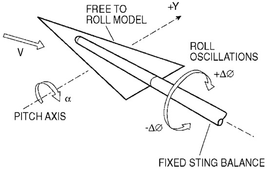
Figure 1.
Schematic view of the delta-wing free-to-roll experiment [5].
Siemens Star-CCM+ mesh generation procedure is robust and quick from simple to complex geometries as shown in [27]. The considered plan for the numerical simulations involves both static and dynamic tests of the delta wing, which requires a body-fitted grid to be rotating around a prescribed center of rotation. Therefore, all simulations were conducted using an overset/chimera method that is robustly implemented in Star-CCM+ CFD code [25]. This, in turn, means that the computational grid consisted of two domains; the first domain was for the overset mesh region consisting of the delta wing placed in a rectangular box, hereafter named the “overblock zone”. The second domain consisted of the wind tunnel, hereafter named the “background zone”. The overblock zone’s dimensions were carefully chosen as away in each direction from the center of rotation and away in the downstream direction. This allowed us to refine the near wake region in a more efficient way. One requirement for the adopted meshing approach with the overset method is that overset interface between the two zones should have similar spacing. This is to allow smooth data interpolation of the flow variables between the two cell zones.
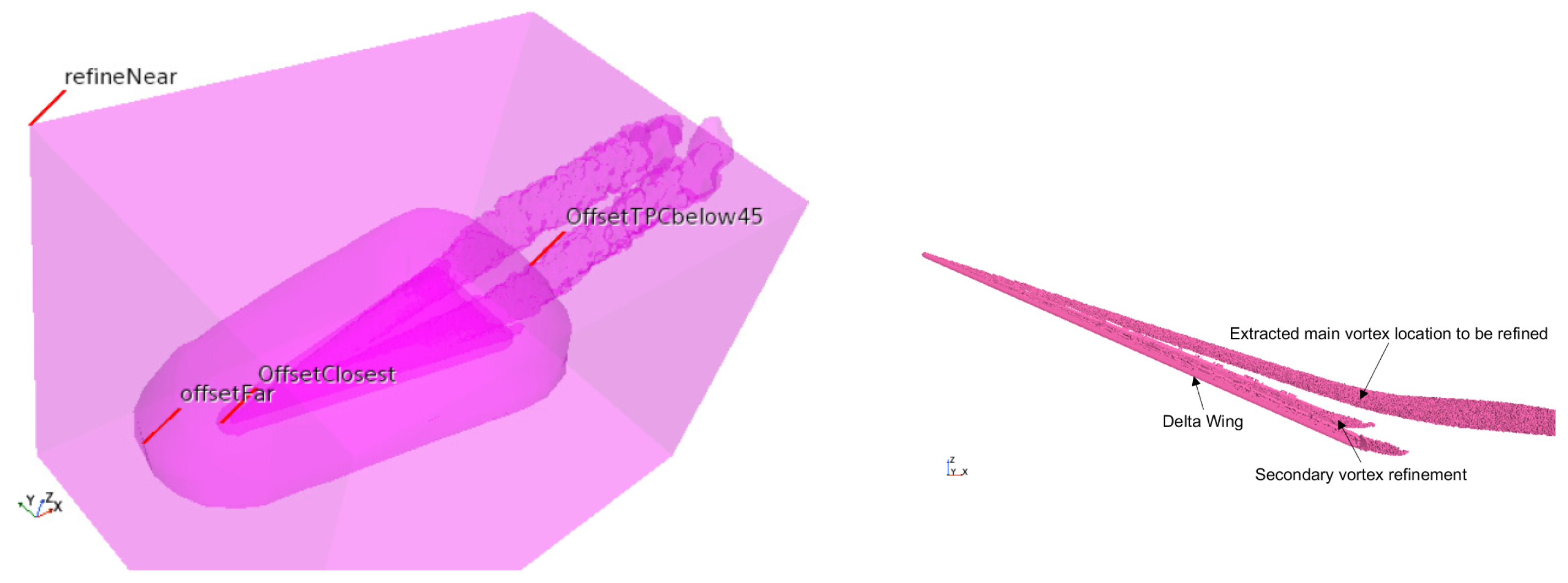
Several refinement strategies were considered in the initial mesh build-up phase in order to make sure that the vortex dynamics, along with the strength and vortex pair interaction, was accurately captured. Some of these strategies, including the extraction of an iso-surface of the vortex based on total pressure coefficient from a coarse grid simulation along with volume offsets of the delta wing, are shown in Figure 2. An isometric view of the grid generated for and a section plane mesh view through the symmetry of the delta wing are shown in Figure 3.
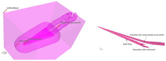
Figure 2.
Refinement strategies including extraction of the vortex location using an iso-surface of the total pressure coefficient for the 80-degree delta wing at .
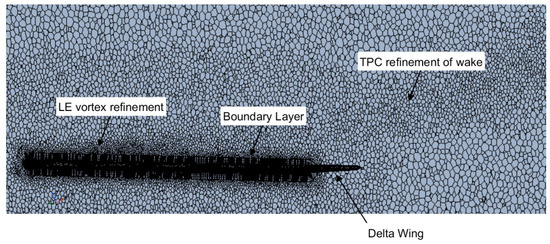
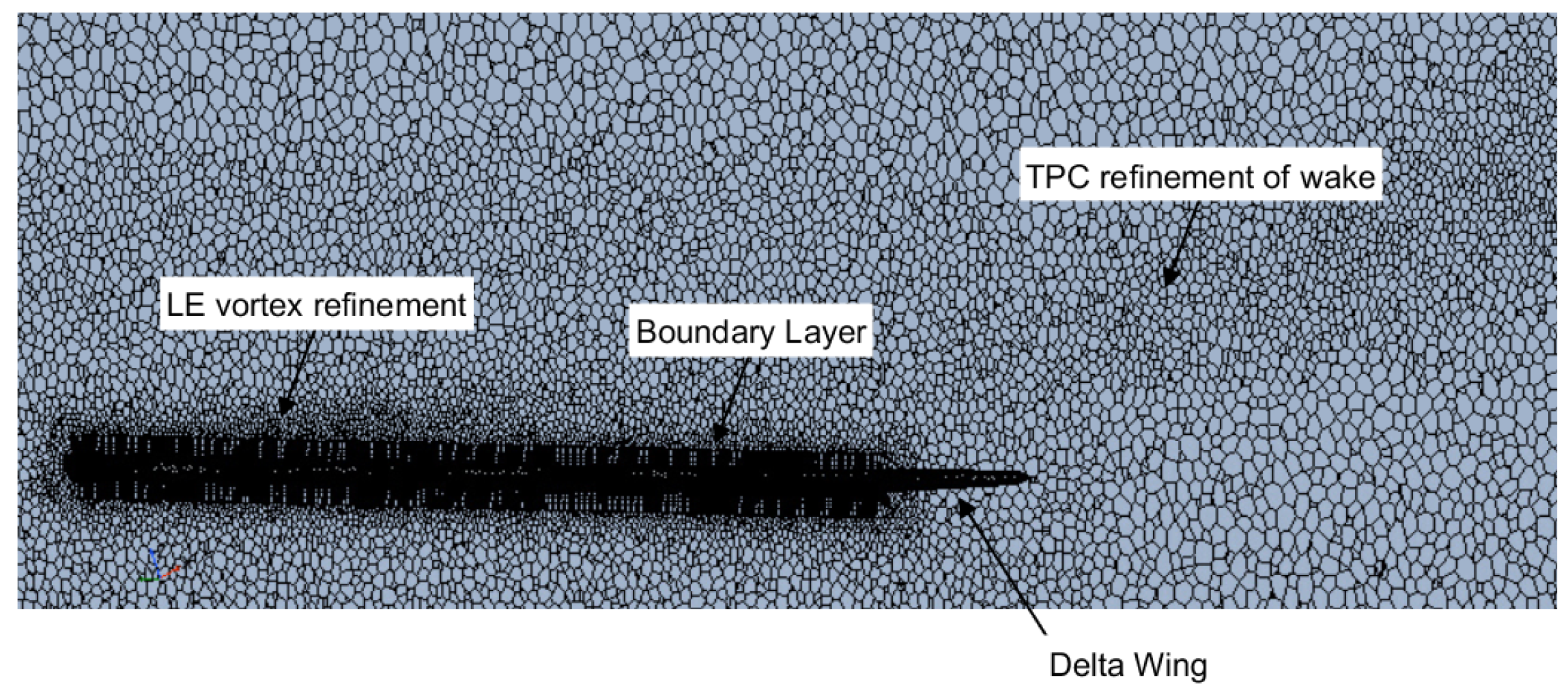
Figure 3.
Adopted grid for the 80-degree delta wing at .
2.2. Numerical Solver Setup
The continuity, momentum, and turbulence equations were solved in a segregated manner using the Algebraic Multi-Grid (AMG) solver with an inner tolerance of , solving the matrix holding the discretized finite volume coefficients to an order of at least 3 decades. The V and F cycle approach was employed with 2 pre- and post-sweeps in order to maximize convergence. For the multi-grid method, the restriction tolerance was kept at and the prolongation tolerance was kept at . It was also necessary to employ some extent of under-relaxation of flow variables, especially for the high-angle-of-attack flows with the vortex breakdown phenomenon and the wing-rock simulations.
Although the grids were intentionally constructed using a low wall approach, i.e., , Star-CCM+ recommends using “All treatment”. With this wall treatment method, boundary layers that meets the low criterion are resolved using the low approach, and boundary layers that violate the low criterion are resolved using the high wall treatment method. The gradients of conservative flow parameters are solved with the second order of accuracy along with the Venkatakrishnan method [28], which limits spurious oscillations in the flow field.
2.3. Mesh Independence Study at
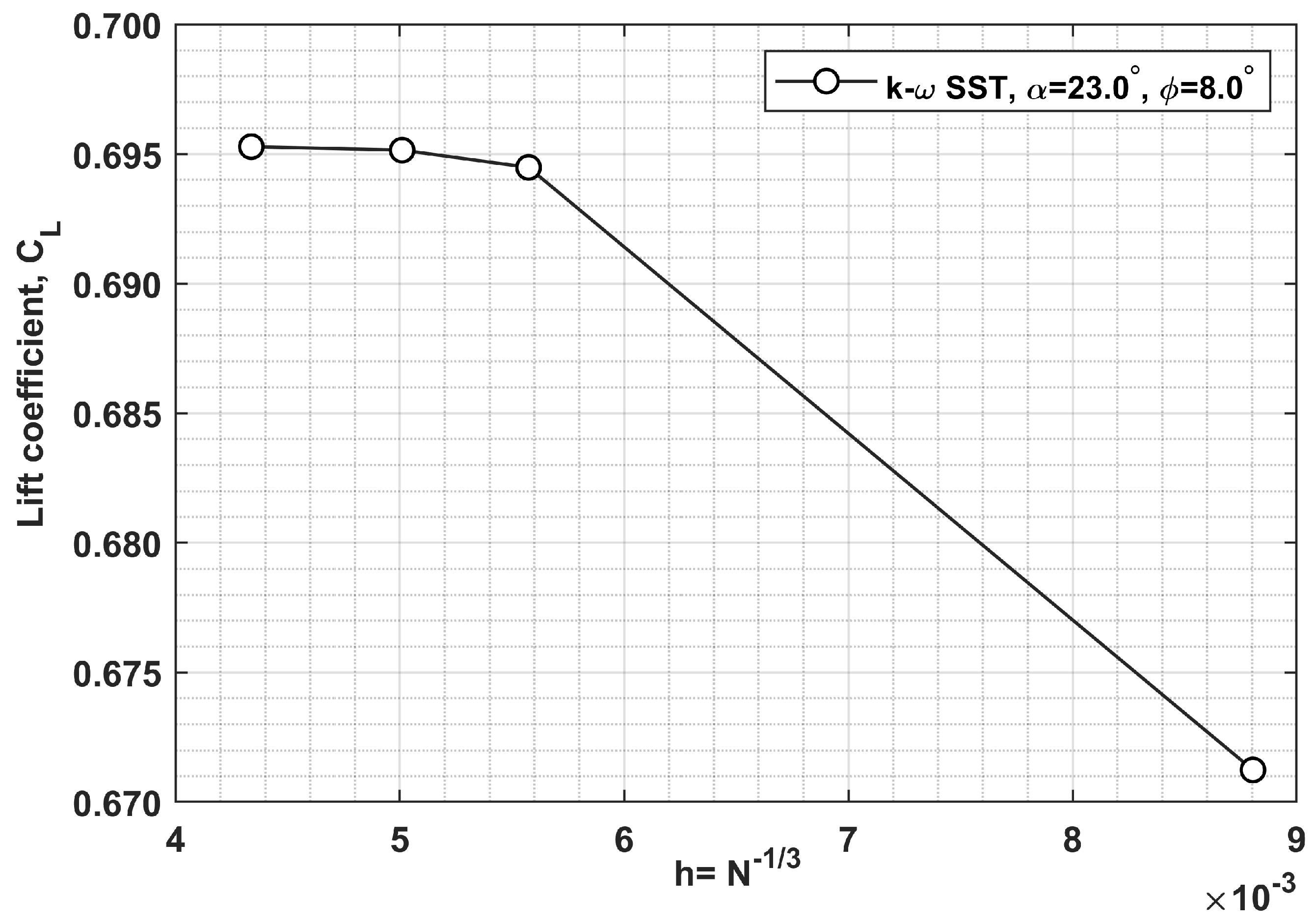
A mesh independence study was conducted to determine the level of refinement required to obtain a grid-independent solution. The computations were carried out at and . The obtained results for the lift coefficient depending on the number of elements in the grid are shown in Figure 4. The computational results obtained from URANS simulations in conjunction with the Shear Stress Transport (SST) turbulence model [29] carried out at and demonstrated that the obtained solution was independent of the grid beyond approximately million elements. Note that for higher-angle-of-attack simulations, a comparison between SST and SST Delayed Detached Eddy Simulations (SST-DDES) is provided in this paper.

Figure 4.
Variation of the lift coefficient with the grid refinement parameter h where N equals the no. of grid elements at and .
2.4. Dynamic Fluid–Body Interaction Framework
The Dynamic Fluid–Body Interaction (DFBI) framework allows a rigid body to undergo free or constrained motion depending on fluid forces acting on the body and/or external forces applied on the fluid and body [25]. In this subsection, the theory of the DFBI motion framework, along with the setup used to for the free-to-roll motion of the 80-degree delta wing, is briefly discussed.
The free motion of a body with a fixed mass and the resultant forces acting in a local coordinate system can be expressed as follows:
where M in Equation (1) is the tensor of the moments of inertia, is the angular velocity of the body, and n is the resultant moment acting on the body [25].
More precisely, herein, we are focused on the 1-DOF rotation that allows a free-to-roll motion around the body x-axis of the wing. This type of motion can be described as follows:
A coupled system of equations for the free-to-roll wing motion under aerodynamic loads arising from this motion and predicted by the Unsteady Reynolds-Averaged-Navier–Stokes (URANS) equations is used to simulate the wing rock of an 80-degree delta wing at various given angles of attack. The obtained results of these simulations and their analysis are presented in Section 4. It should be noted that the friction moment in the wing bearings was considered negligible.
In Equations (4) and (5), is the specified angular damping length. For this particular case study, and other tensor components are dependent on the moment of inertia, and they were obtained through the Star-CCM+ CFD code using the inbuilt functions. The obtained moments of inertia were based on a density of 1 kg/m3 and therefore were corrected to reflect the actual density of the delta wing in the experimental data presented in [10]. The 80-degree delta wing in the experiment was made up of duralumin material. A summary of the wing dimensions and moment of inertia is presented in Table 1.

Table 1.
Reference data for the 80-degree delta wing.
3. Predicting the Onset of Self-Oscillations of a Delta Wing
As the angle of attack increases, the vortices that shed from a delta wing’s leading edge move vertically away from the wing surface and become more intense. In free-to-roll wing motion, the conical vortices lag behind in position and intensity compared to their state under static conditions. At some angle of attack, the time delay in the vortices’ position and strength produces a destabilizing effect on the wing motion, leading to the onset of oscillatory instability and the development of self-sustained oscillations, known as the wing-rock phenomenon.
The amplitude of the wing-rock oscillations reaches a maximum at a certain angle of attack and begins to decrease due to flow transformation influenced by the onset of vortex breakdown [21]. The experimental results in [10] show the existence of two modes of self-oscillation of the 80-degree delta wing, namely, large-amplitude regular oscillations and small-amplitude irregular or chaotic oscillations at . The co-existence of these two modes of wing self-oscillations requires a deeper understanding of the wing–vortex interaction during small-amplitude and large-amplitude self-oscillations. For this purpose, in this section we implement numerical simulation of static tests, forced oscillation tests, and rotary balance tests commonly used in a wind tunnel, which will provide information on the wing’s oscillatory instability and the cause of chaotic self-oscillations during free-to-roll motion.
3.1. Computational Analysis of the Stability of Free-to-Roll Wing Motion
Free-to-roll wing motion is described by the following second-order differential equation for one degree of freedom:
where is the wing’s moment of inertia, is the air density, V is the free stream velocity, S is the wing area, and b is the wing span. Traditionally, the rolling moment coefficient depends on the wing motion parameters, on the roll angle (in fact, on the sideslip angle ), and on the angular velocity . To analyze wing motion stability in this section, we use the standard representation of the rolling moment coefficient , considering its dependencies on angle of attack , sideslip angle , conical rotation rate , and its aerodynamic derivative . A modified phenomenological lag and relaxation model for wing–vortex interaction and its effect on free-rolling oscillations was given in [30].
3.2. Static Tests
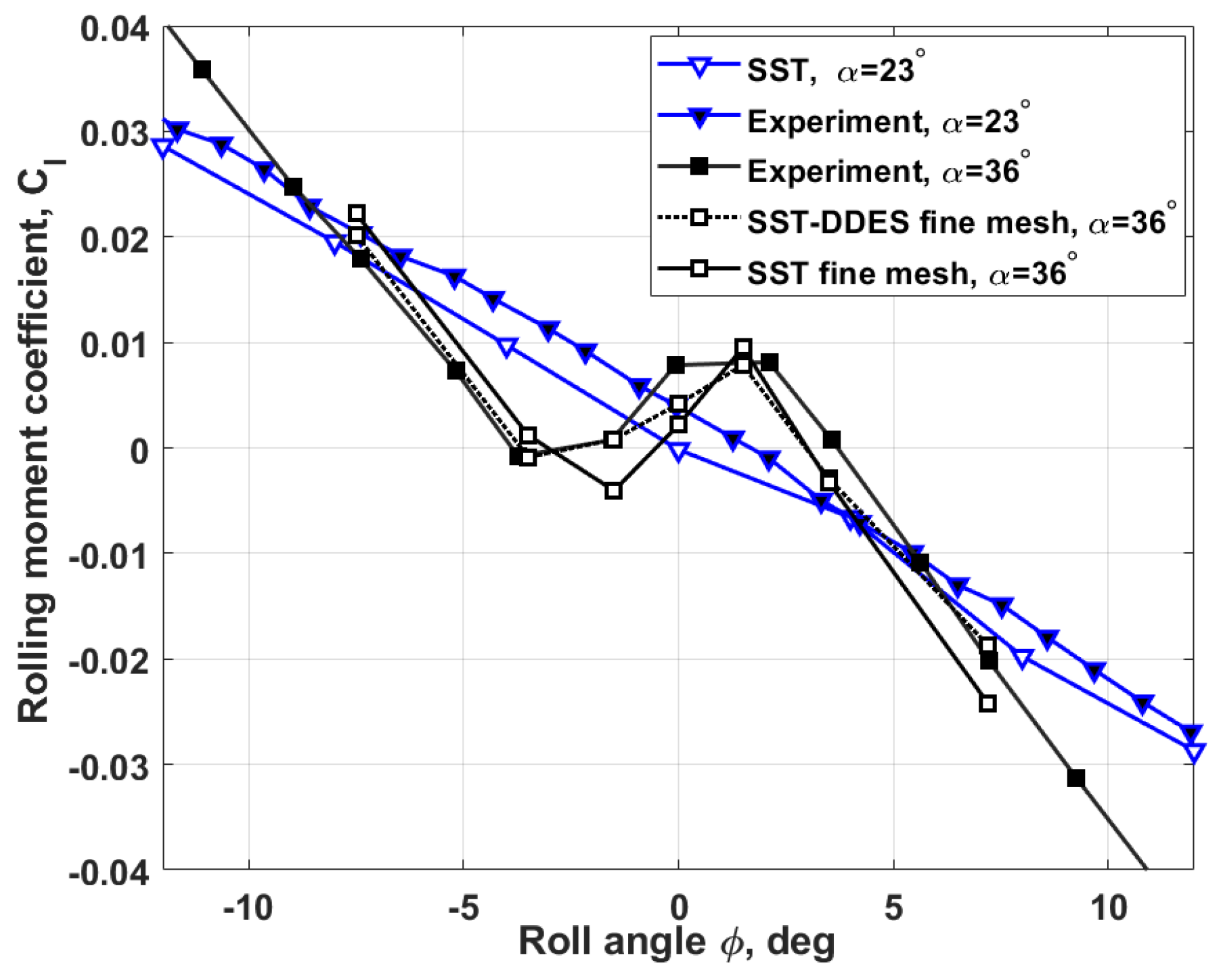
The computed rolling moment coefficients in the static state are compared in Figure 5 with the experimental results from [10] for two angles of attack: and (note that the sideslip angle is proportional to the rolling angle ). Numerical simulation of static states was carried out using the URANS equations with a very slow change in the rolling angle, at a rate of °/s, and showed good qualitative and quantitative agreement with the experimental data.
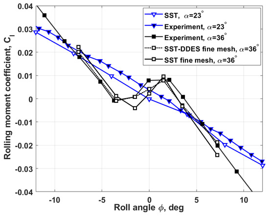
Figure 5.
Dependencies of the rolling moment coefficient for and : results of the simulation and experiment from [10].
At low angles of attack, the rolling moment derivative shows that the wing in free-to-roll motion is statically stable. Its magnitude increases with the angle of attack , showing practically linear dependence of the rolling moment on the sideslip angle (blue lines with triangle markers at ). With an increasing angle of attack, the interaction of the wing with the vortex leads to oscillatory instability in free-to-roll motion. The occurrence of oscillatory instability can be determined by the change in sign from negative to positive in the rolling moment derivative , where p is the angular velocity of the roll and is the rate of change of the sideslip angle (see Figure 6).
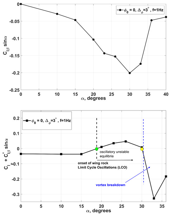
Figure 6.
Predicted in-phase and out-of-phase aerodynamic derivatives from CFD simulations (the upper and lower graphs, respectively) vs. angle of attack.
At some angle of attack, the onset of vortex breakdown changes the sign of the static aerodynamic derivative from negative to positive at zero sideslip and generates two non-zero equilibrium positions of the wing with a negative slope of the rolling moment, . The vortex breakdown makes the symmetric position of the wing in free-to-roll motion statically unstable and creates two asymmetric equilibrium states that are statically stable (see black lines with square markers in Figure 5 for ). This transformation of the rolling moment coefficient is described by the so-called pitchfork bifurcation [1,24].
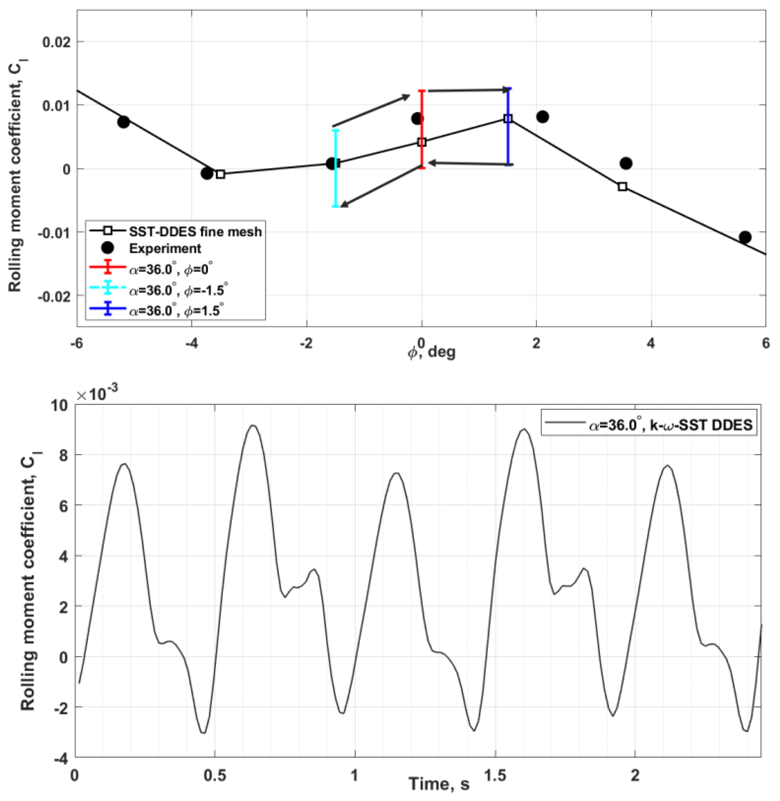
The static dependence at , obtained in the numerical simulation by averaging over time, is somewhat asymmetric, as in the experiment, in both cases having three equilibrium points determined by the zero points of the rolling moment coefficient (Figure 5). The rolling moment coefficient of an 80-degree delta wing at and zero sideslip, obtained using the URANS equations, oscillates at a frequency of Hz, indicating the existence of aerodynamic buffet (see the time history of in Figure 7, lower graph). The shown aerodynamic buffet regime exists in a narrow range of sideslip angles, , and has a non-zero positive mean amplitude, which means that another buffet regime with a mean value of the opposite sign will also exist, leading to a static hysteresis dependence (see the dependence in Figure 7, upper graph).
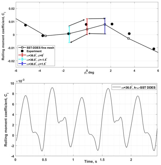
Figure 7.
Hysteresis of aerodynamic buffet due to vortex breakdown. Simulated and experimental results for the rolling moment coefficient at .
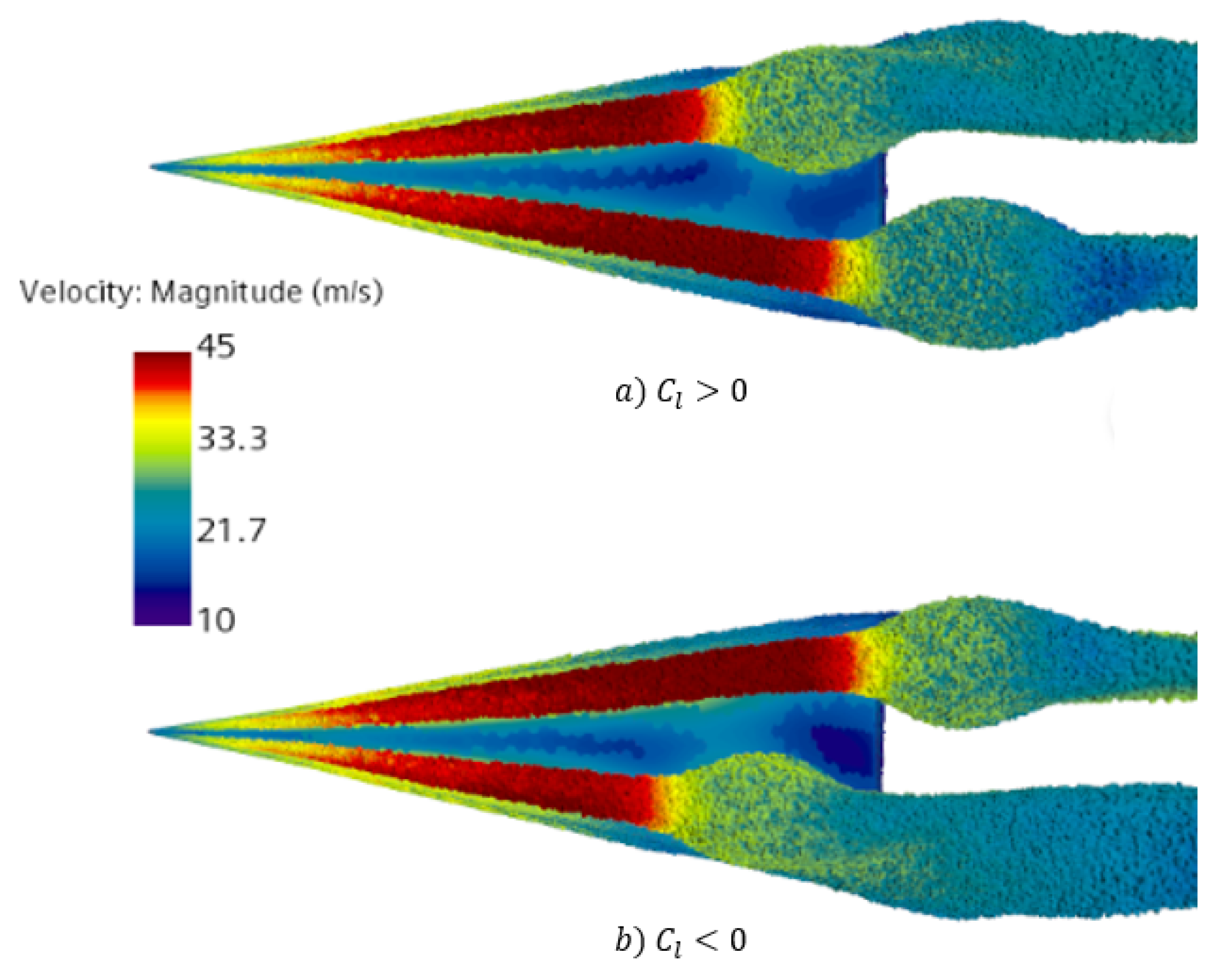
Flow visualization of the computed flow field with leading-edge vortices is presented in Figure 8, Figure 9 and Supplementary Materials, respectively, for the pressure and velocity contours. Figure 8 shows the distribution of the pressure coefficient on the wing surface and the leading-edge vortices at and bank angle in static conditions. One can see that there is very low pressure in the vortex cores, which are slightly asymmetric at zero sideslip angle . Figure 9 shows a top view of the vortex breakdown above the wing at two time points with the maximum and minimum magnitudes of on the buffet time history presented in Figure 7.
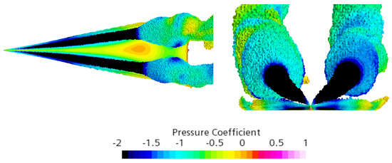
Figure 8.
Contours of the distribution of the pressure coefficient on the vortices and the wing surface at and bank angle in static conditions (top and front views).

Figure 9.
Top-view flow visualization of wing vortices at and bank angle (velocity magnitude for the vortices and contours of the pressure coefficient on the wing surface).
3.3. Forced Oscillation and Conical Rotation Tests
To predict the occurrence of oscillatory instability of the wing, the variation of the rolling moment coefficient acting on the moving wing was simulated using the URANS equations for harmonic oscillations with a given mean value , amplitude , and frequency f. This modeling is identical to forced oscillation tests in a wind tunnel, and we used the same procedure to extract the in-phase and out-of-phase aerodynamic derivatives.
With a periodic change in the roll angle , the rolling moment coefficient after a transient process also becomes periodic in time , where . After convergence to a periodic process, the rolling moment coefficient is approximated by the first terms of the Fourier series, which makes it possible to obtain in-phase and out-of-phase aerodynamic derivatives:
Comparing (7) with the usual representation of the rolling moment coefficient in the form of aerodynamic derivatives,
the in-phase and out-of-phase aerodynamic derivatives can be linked with the first terms of the Fourier series, and :
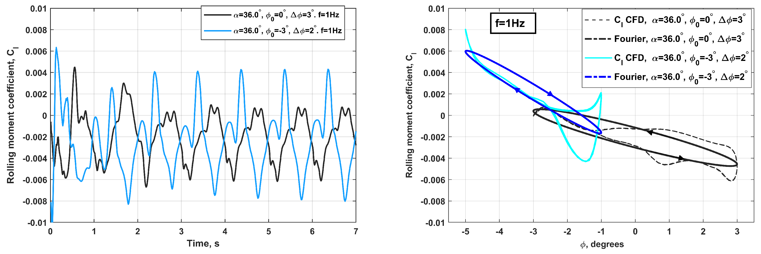
Numerically simulated processes for the rolling moment coefficient during forced oscillations in roll at with , and , at a frequency Hz are shown in Figure 10 (left graph). The Fourier series for the rolling moment coefficient (7) is applied after the convergence to a periodic process at s, which also includes high-frequency oscillations produced by the buffet of vortex breakdown.
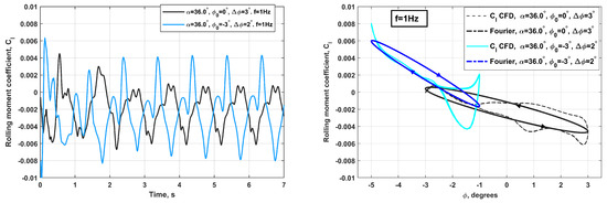
Figure 10.
Numerical simulation of the rolling moment coefficient as a function of time for small-amplitude wing oscillations in roll at with , and , (left graph). Elliptic approximation of the cycle by only the first harmonic of the Fourier expansion (right graph).
The simulated rolling moment coefficient processes shown in Figure 10 (right graph) are plotted against the roll angle variation . The first two terms of the Fourier series (7) approximate these processes as harmonically equivalent ellipses. The slope of an ellipse’s major axis defines the in-phase aerodynamic derivative , while the size of the minor axis and the direction of rotation define the out-of-phase aerodynamic derivative . Clockwise rotation means that the out-of-phase derivative is negative, and counterclockwise rotation means that the out-of-phase derivative is positive. The two Fourier ellipses shown in Figure 10 (right graph) for have rotations in opposite directions, which means that the asymmetric equilibrium state of the wing at has oscillatory instability, since , and at the out-of-phase derivative is negative ().
The aerodynamic derivatives obtained in phase and out of phase for are shown in Figure 6 for a range of angles of attack. The out-of-phase aerodynamic derivative in Figure 6 (lower graph) can be used to predict the oscillatory stability of the wing in its free-to-roll motion. At a low angle of attack, , the out-of-phase aerodynamic derivative for an 80-degree delta wing remains negative (). This means that the wing is dynamically stable and will converge to its zero-roll position after being given initial disturbances. The onset of oscillatory instability occurs at when the out-of-phase derivatives become positive (green circle). Generally, steady self-oscillations start at , and the amplitude grows with the absolute magnitude of the out-of-phase aerodynamic derivative, characterizing the intensity of the oscillatory instability of the wing. This type of transformation of the stable zero equilibrium of the wing in its free-to-roll motion is described by the so-called supercritical Hopf bifurcation [1]. This bifurcation indicates the onset of oscillatory instability of the equilibrium point with the simultaneous onset of a stable limit cycle characterizing the self-oscillations of the wing.
The change in the sign of from positive to negative occurs at an angle of attack of , just before the start of the vortex breakdown when the zero equilibrium becomes aperiodically unstable. This type of transformation of the equilibrium of the wing during its free motion is described by the subcritical Hopf bifurcation [1], which generates a saddle-type limit cycle, the role of which is to separate two different attractors that characterize the dynamics of the wing with a vortex breakdown.
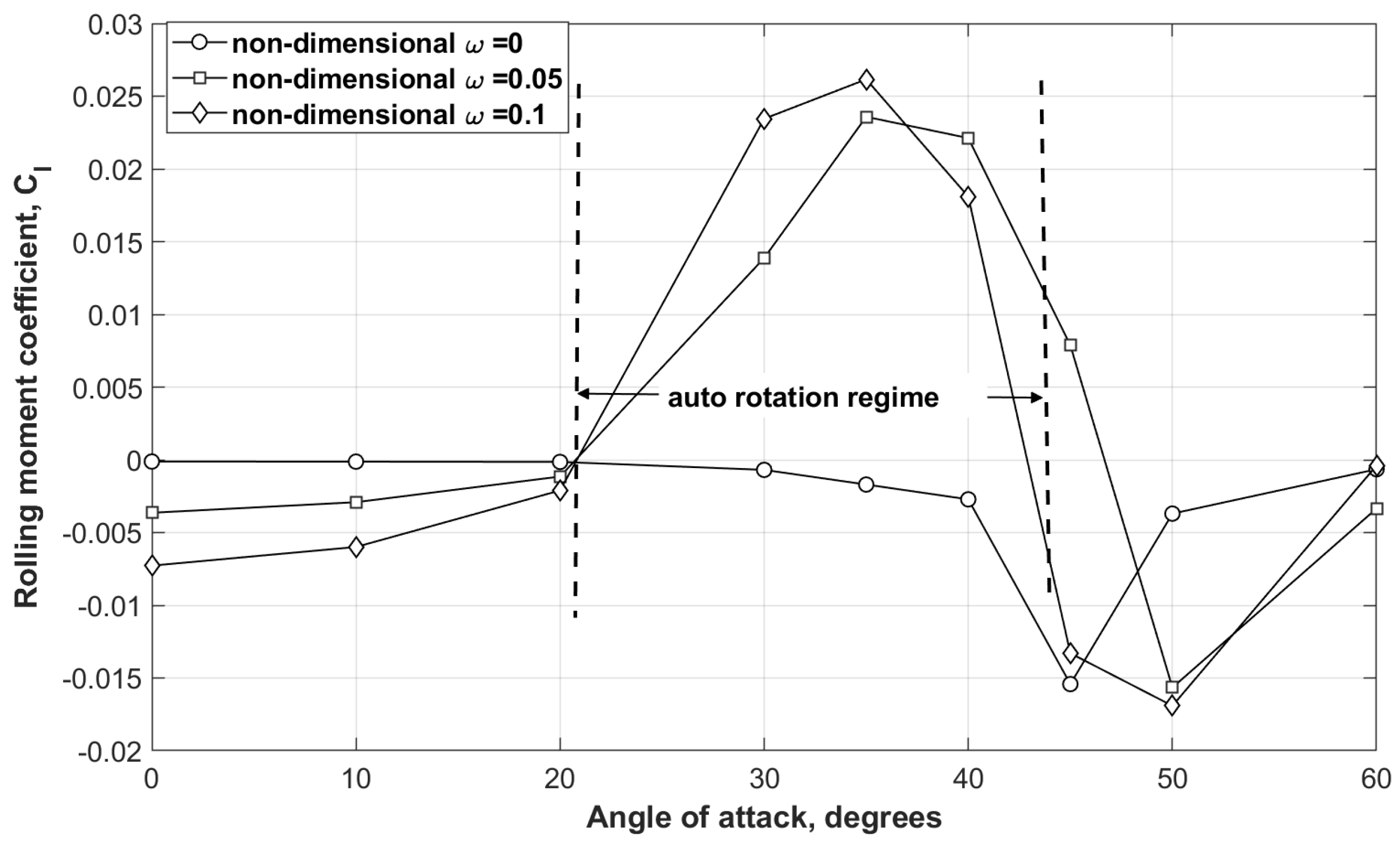
The effect of aerodynamic autorotation in a wind tunnel was investigated in rotary balance tests by analyzing the dependence of the rolling moment on the speed of conical rotation around the velocity vector. The results of numerical simulations for different angles of attack, similar to the rotary balance tests in a wind tunnel, are presented in Figure 11. For zero rotation (), the simulation results show asymmetric rolling moments at high angles of attack, , due to asymmetric vortex breakdown, which reaches its maximum value at . The effect of aerodynamic autorotation occurs at , when the derivative of the rolling moment changes sign from negative to positive. This occurs at an angle of attack three degrees greater than that at which oscillatory instability occurs in the free-to-roll motion of the wing.
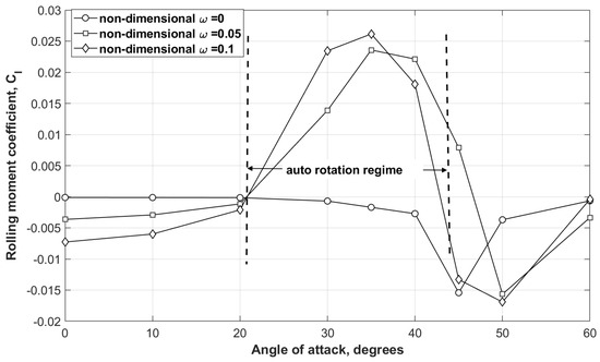
Figure 11.
Rolling moment coefficient vs. angle of attack for different reduced rotation rates with conical motion around the velocity vector from CFD simulations: , and .
For adequate simulation of a vortex flow with intense concentrated vortices, which are typical of small and medium angles of attack and the breakdown of vortices at high angles of attack, it is important to use a correctly created grid that covers vortex cores and breakdown regions. A sufficiently fine grid ensures realistic simulation of flow parameters with intense concentrated vortices and gives dependencies of aerodynamic coefficients that are very close to the experimental results. The simulation results with a medium mesh containing about 5.5 million elements, which was found to be sufficient in the mesh independence study at , failed to predict a nonlinear relationship for the rolling moment coefficient at , as shown in Figure 5. To improve the computational fluid dynamics predictions in this case, refined meshes with approximately 8–9 million elements were constructed, with particular attention paid to refining the vortex cores using a threshold value for the total pressure coefficient. This improvement allowed us to capture the same nonlinear trends in the rolling moment coefficient as in the experiment using both the SST URANS approach and the SST Delayed Detached Eddy Simulation (DDES) approach.
4. Coupled Fluid–Rigid Body Simulation of Wing-Rock Motion
Simulation of the free-to-roll motion of the wing was carried out using a coupled system of equations describing the movement of the wing under the action of aerodynamic loads, predicted by simultaneously solving the Unsteady Reynolds-Averaged-Navier–Stokes (URANS) equations. The results of the simulation and an analysis of these results are presented in this section. The aerodynamic loads, including distributed pressure and viscous forces, were evaluated at each time step and used to transform the body-fixed grid in the overset region according to the moment of inertia tensor. The friction moment in the wing bearings was considered negligible.
Wing-Rock Simulations at Various Angles of Attack
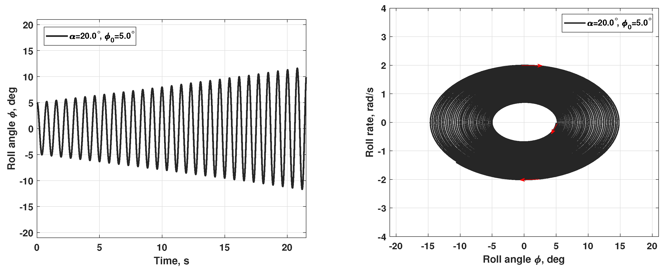
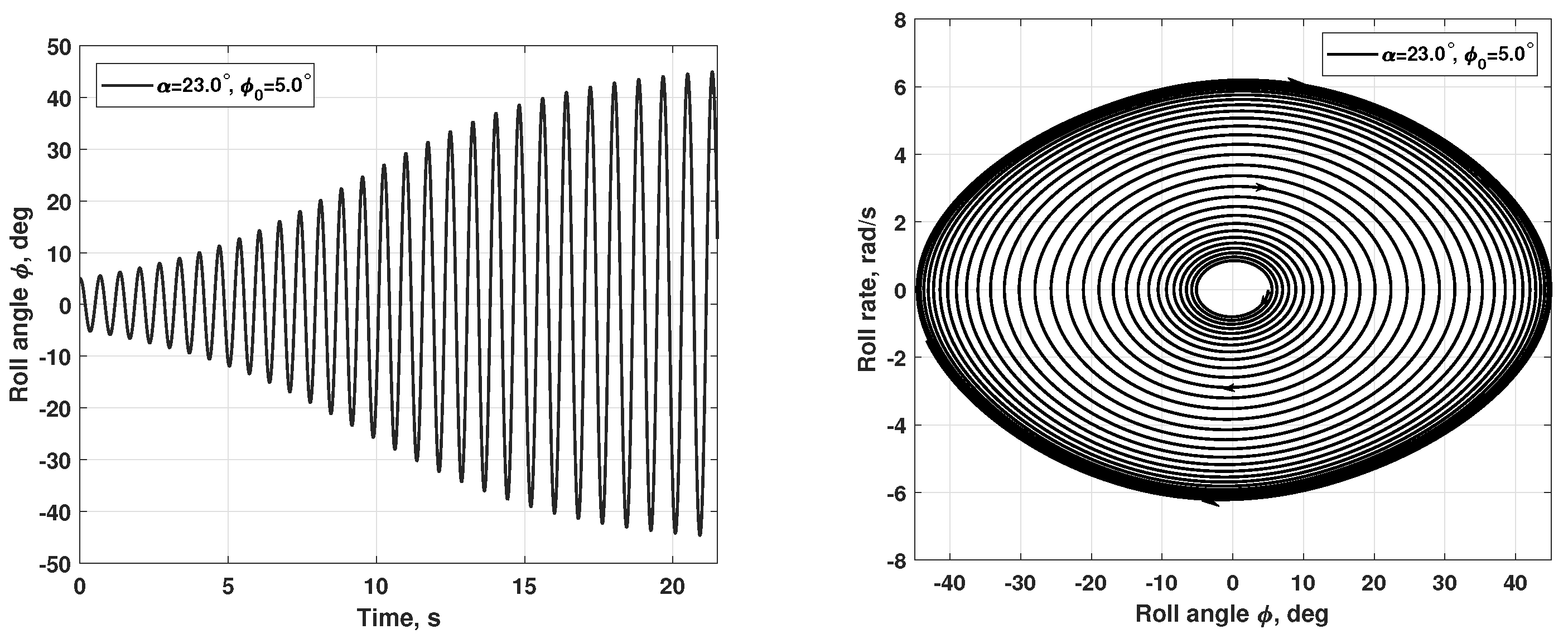
Simulation of wing-rock motion was performed for a number of angle-of-attack settings (, and ) to illustrate different types of wing behavior predicted based on the out-of-phase derivative (Figure 6). The simulation process for in the form of the time history and the phase portrait vs. is shown in Figure 12. The motion of the wing is stable; rather fast damping of the oscillation amplitude and convergence to the neutral equilibrium state are observed. This type of behavior correlates well with the predicted value of the aerodynamic derivative for . At an angle of attack of , the wing motion shows oscillatory instability due to the sign change of the aerodynamic derivative to positive. The process for this case, shown in Figure 13, has a very slow increase in oscillation amplitude without convergence to a steady wing motion over a given time interval. At a larger angle of attack (), the intensity of oscillatory instability () is more than three times higher than at . The simulated time history and phase portrait for this angle of attack are shown in Figure 14. The increase in amplitude occurs more intensively with saturation in steady-state oscillations over a time interval of 20 s. The amplitude of the steady oscillations of the wing is approximately 40 degrees.
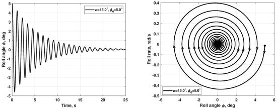
Figure 12.
Simulated time history (left graph) and phase portrait (right graph) of the 80-degree delta wing in free-to-roll rotation at angle of attack with initial roll angle .
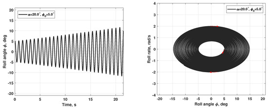
Figure 13.
Simulated time history (left graph) and phase portrait (right graph) of the 80-degree delta wing in free-to-roll rotation at angle of attack with initial roll angle .
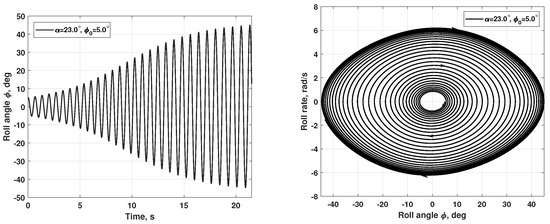
Figure 14.
Simulated time history (left graph) and phase portrait (right graph) of the 80-degree delta wing in free-to-roll rotation at angle of attack with initial roll angle .
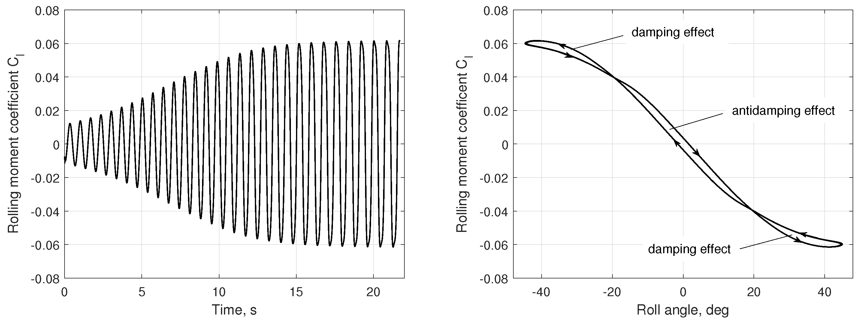
The time history of the rolling moment coefficient and the twisted loop showing the dependence between the rolling moment coefficient and the roll angle for are presented in Figure 15. Variation of the rolling moment coefficient in the form of a twisted loop in Figure 15 (on the right) corresponds to the end of the oscillatory process with practically maximal amplitude of a saturated wing-rock motion. The section in the middle of the loop showing the passage of time in a clockwise direction (energy extraction from the flow) is compensated by two sections at the ends of the loop with a counterclockwise course of time (energy is dissipated from the wing), which indicates the balance of energy for the interval of one oscillation cycle.

Figure 15.
The rolling moment coefficient vs. time (left graph) and the rolling moment coefficient vs. roll angle (right graph) of the 80-degree delta wing in free-to-roll rotation at angle of attack with initial roll angle .
The free roll oscillations of the wing change significantly at due to the onset of the vortex breakdown. Regular oscillations of large amplitude remain, but small-amplitude oscillations also appear; the latter have an irregular or “chaotic” character. The excitation of one of these types of motion depends on the initial roll angle.
Chaotic oscillations are generated between two equilibrium states of the wing that are opposite in sign, arising after the breakdown of the vortices. These two equilibria (see Figure 5) show oscillatory instability, but after the increase in oscillation amplitude around an equilibrium point, the wing jumps to an opposite equilibrium point that also shows oscillatory instability, and this process is continuously repeated in time, having a chaotic character. A more detailed analysis of this mechanism can be found in [30].
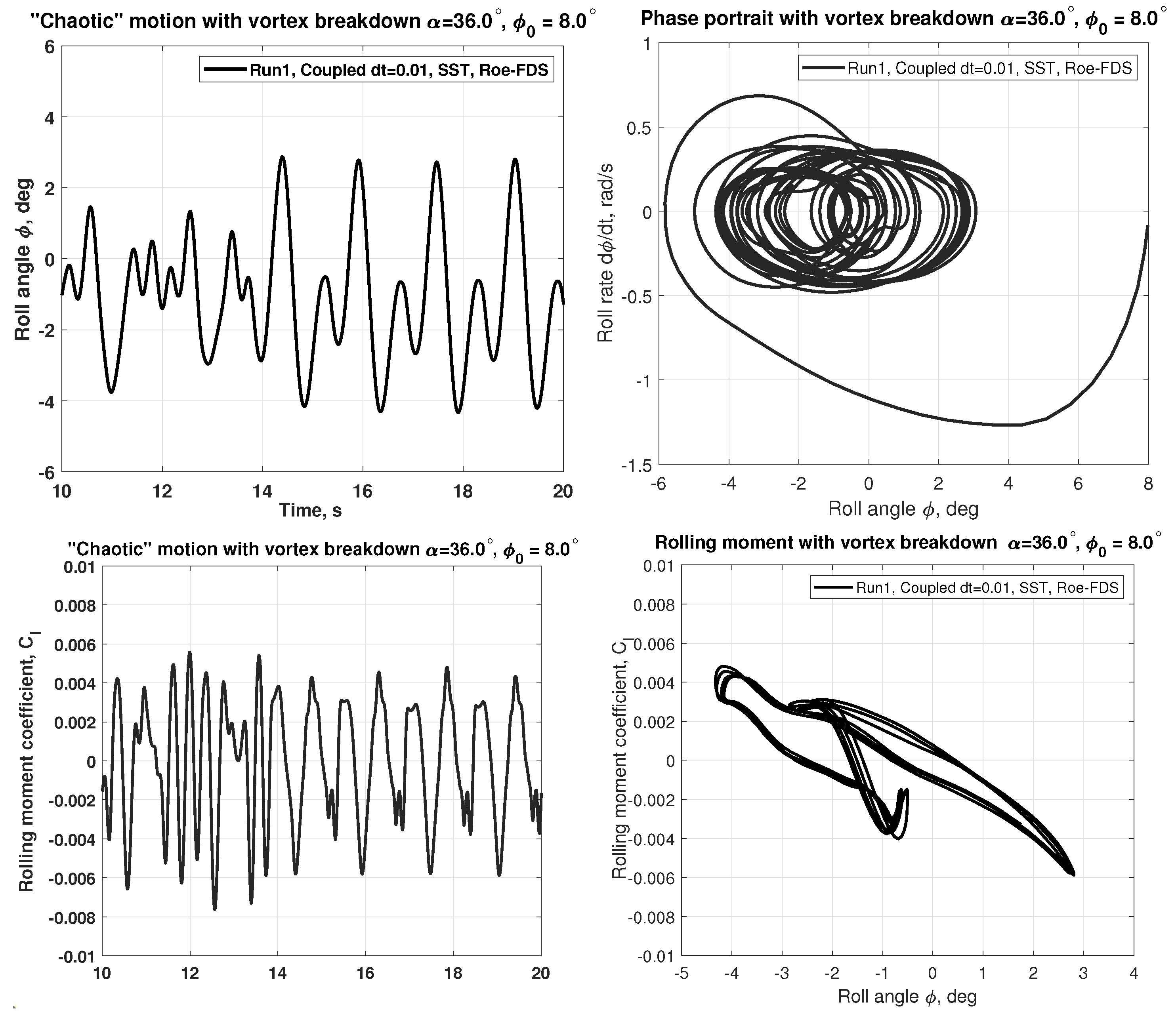
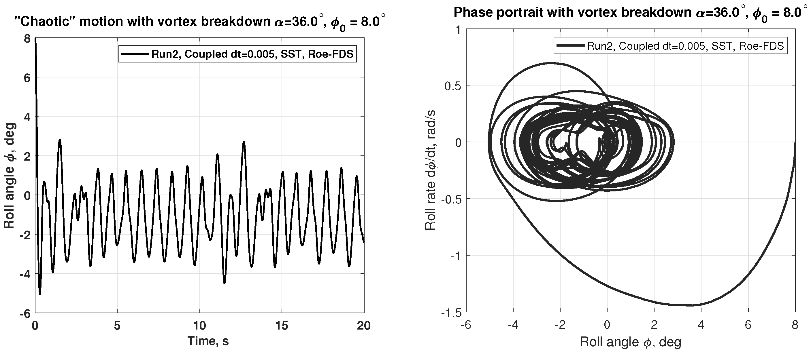
These chaotic oscillations of the wing are very sensitive to any numerical changes introduced into the system, for example, to the integration time step, initial conditions, etc. Simulation of “chaotic” oscillations of the wing, initiated at the same initial roll angle but with different time integration steps and , are shown in Figure 16 and Figure 17, respectively. A coupled flow solver with inviscid flux approximated by Roe Flux-Difference Splitting (Roe FDS) was used in both simulations. It is clearly seen that the temporal characteristics of the roll angle and the phase portrait in these two simulations are somewhat different but retain their chaotic nature and the magnitude of their amplitudes.

Figure 16.
Simulation results for “chaotic” free-to-roll oscillations of the 80-degree delta wing at with initial roll angle : roll angle time history (upper left plot), phase portrait (upper right plot), rolling moment coefficient time history (lower left plot), and vs. roll angle (lower right plot). Time step used in simulation s.
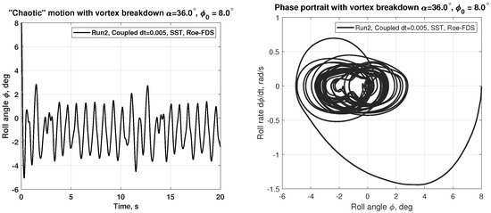
Figure 17.
Simulation results for “chaotic” free-to-roll oscillations of the 80-degree delta wing at with initial roll angle : roll angle time history (left plot) and phase portrait (right plot). Time step used in simulation s.
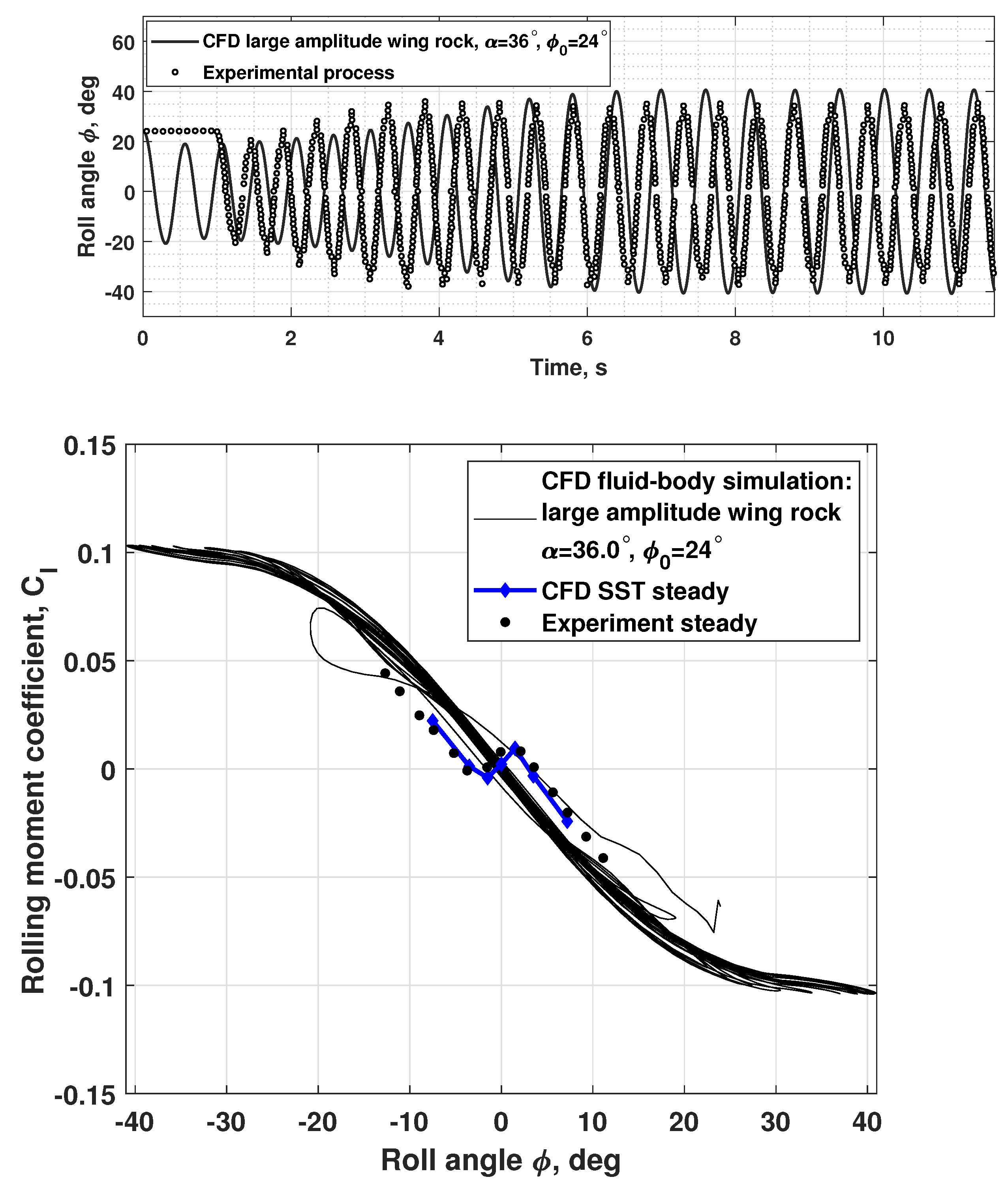
When the initial bank angle increases to , the delta wing goes into a large-amplitude oscillation mode with a maximum bank angle of , which is similar to what occurs at . Figure 18 shows the simulation results in comparison with experimental data from [10]. The time history of the bank angle (upper graph) from numerical simulation is very close to the experimental data, shown by empty circles, in terms of amplitude and period length. The change in the rolling moment coefficient during these oscillations in comparison with its static dependence versus the roll angle, shown earlier in Figure 5, indicates that vortex breakdown does not occur during large-amplitude oscillations Figure 18 (lower graph). This may be due to changes in flow conditions at high angular velocities, which might prevent the occurrence of vortex breakdown phenomena.
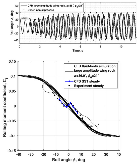
Figure 18.
Computational and experimental results showing the rolling moment coefficient versus roll angle (lower graph) and the roll angle time history (upper graph) of large-amplitude oscillations of an 80-degree delta wing at , .
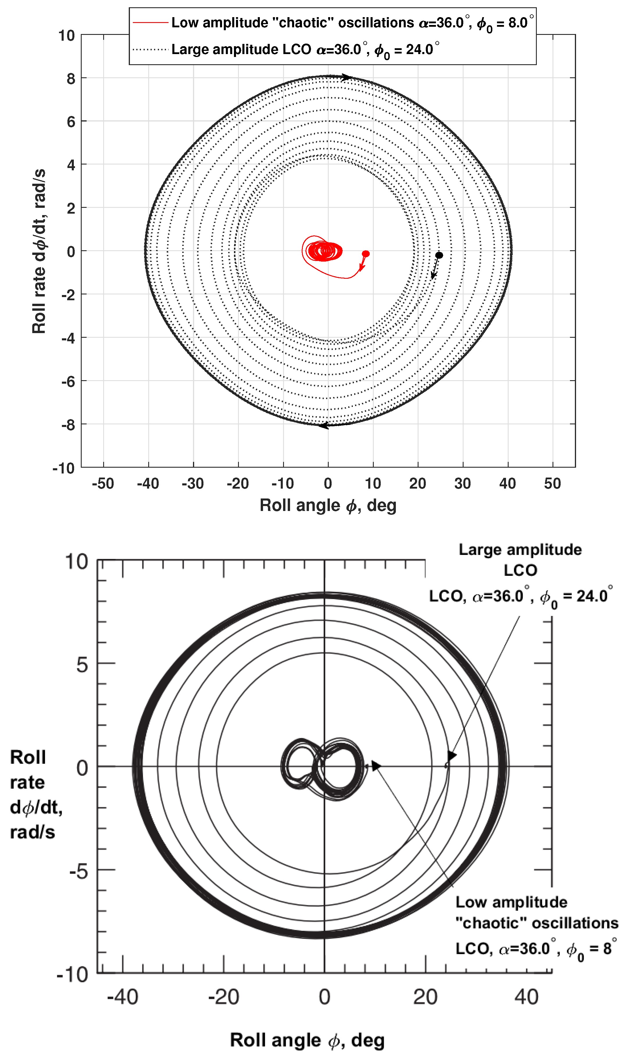
Figure 19 (upper graph) shows a phase portrait combining trajectories for large-amplitude oscillations and “chaotic” small-amplitude oscillations, obtained in numerical simulations using two different initial conditions for the bank angle. Figure 19 (lower graph) shows a similar phase portrait composed of experimental data [10]. Good qualitative and quantitative agreement are seen between the free-to-roll wing oscillations predicted by CFD and those obtained in the experiment, with both clearly demonstrating two stable delta wing oscillation modes at . The boundary between the basins of attraction for these two modes separates the wing dynamics influenced by the vortex breakdown in the inner region and the wing dynamics influenced by the unbroken vortices in the outer region of the phase portrait. The trajectory that starts at a bank angle of is self-intersecting in the planar phase portrait in both the experiment and the computational fluid dynamics simulation, indicating the presence of additional dynamics due to flow delays during the wing motion. This observation confirms that a common representation of the rolling moment coefficient in Equation (6) based on aerodynamic derivatives should be modified, for example, as presented in [30].
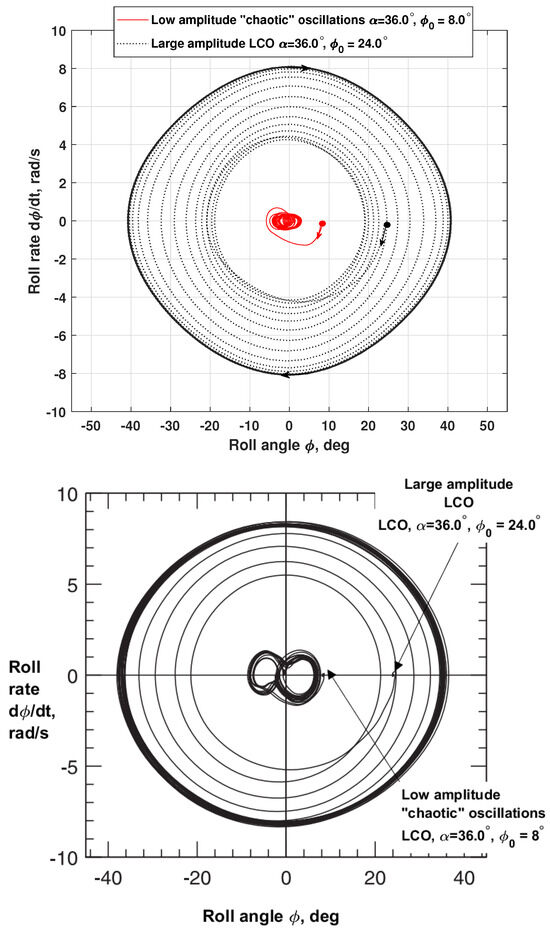
Figure 19.
Numerically simulated and experimental phase portraits for (upper and lower plots, respectively), showing two trajectories with initial conditions and converging to different attractors.
5. Conclusions
Numerical simulations of the free-to-roll motion of an 80-degree delta wing under strong wing–vortex interaction were performed with the URANS equations closed by the SST turbulence model using Siemens CFD STAR-CCM+ software. A chimera/displaced mesh method was used in combination with dynamic fluid–body interaction (DFBI).The obtained simulation results allow us to draw the following conclusions:
- To accurately predict the unsteady and nonlinear aerodynamic loads acting on the wing during free-rolling oscillations, a higher-resolution mesh is required due to the existence of intense conical vortices at low and medium angles of attack and due to vortex breakdown at high angles of attack. Mesh refinement is especially needed for vortex cores and vortex breakdown regions.
- Numerical static tests and tests with forced oscillations, similar to those used in a wind tunnel, made it possible to minimize the computer time costs for simulation of coupled wing–vortex oscillations and revealed the nature of the observed chaotic self-oscillations. The obtained aerodynamic derivative with respect to the roll rate, , indicates the onset of self-oscillations of the wing in roll through a change in sign from negative to positive. The vortex breakdown is reflected in a change in the sign of the static aerodynamic derivative from negative to positive and the simultaneous occurrence of two non-zero equilibrium points of the wing.
- The experimental and numerical simulation results, which are in good qualitative and quantitative agreement, both show that the observed two modes of wing self-oscillations in roll at have separate regions of attraction in the space of the wing motion parameters [10]. The chaotic small-amplitude self-oscillations of the wing are closely related to the non-stationary nature of flow due to the lags in vortex breakdown leading to oscillatory instability of two non-zero equilibrium states so that the origin of these self-oscillations is similar to the onset of the strange attractor in the Lorenz system [24]. Along with this, regular oscillations of large amplitude continue to exist at due to the rapid transition through the region with small sideslip angles, which blocks the phenomenon of vortex breakdown.
- The results obtained allow us to conclude that the adopted computational framework of fluid dynamics using the URANS equations and overset mesh generation is capable of adequately modeling complex wing self-oscillations in roll caused by strong wing–vortex interaction.
Supplementary Materials
The following supporting information can be downloaded at: https://www.mdpi.com/article/10.3390/aerospace12030197/s1.
Author Contributions
Conceptualization, M.G. and N.A.; Methodology, M.S. and C.L.; Software, M.S.; Validation, M.S., M.G. and C.L.; Investigation, M.G. and N.A.; Writing—original draft, M.S. and N.A.; Writing—review & editing, M.G. and C.L. All authors have read and agreed to the published version of the manuscript.
Funding
This research received no external funding.
Data Availability Statement
The original contributions presented in this study are included in the article. Further inquiries can be directed to the corresponding author.
Conflicts of Interest
The authors declare no conflicts of interest.
References
- Goman, M.; Zagainov, G.I.; Khramtsovsky, A.V. Application of bifurcation methods to nonlinear flight dynamics problems. Prog. Aerosp. Sci. 1997, 33, 539–586. [Google Scholar] [CrossRef]
- Nguyen, L.; Yip, L.; Chambers, J. Self-Induced Wing Rock of Slender Delta Wings. In Proceedings of the AIAA Atmospheric Flight Mechanics Conference, Albuquerque, NM, USA, 19–21 August 1981. AIAA Paper 81-1883. [Google Scholar]
- Ericsson, L. Wing rock analysis of slender delta wings, review and extension. J. Aircr. 1995, 32, 1221–1226. [Google Scholar] [CrossRef]
- Levin, D.; Katz, J. Self-induced roll oscillations of low-aspect-ratio rectangular wings. J. Aircr. 1992, 29, 698–702. [Google Scholar] [CrossRef]
- Katz, J. Wing/vortex interactions and wing rock. Prog. Aerosp. Sci. 1999, 35, 727–750. [Google Scholar] [CrossRef]
- Arena, A. An Experimental and Computational Investigation of Slender Wings Undergoing Wing Rock. Ph.D. Thesis, University of Notre Dame, Notre Dame, IN, USA, 1992. [Google Scholar]
- Arena, A.; Nelson, R. Experimental investigations on limit cycle wing rock of slender wings. J. Aircr. 1994, 31, 1148–1155. [Google Scholar] [CrossRef]
- Gursul, I. Unsteady flow phenomena over delta wings at high angle of attack. AIAA 1994, 32, 225–231. [Google Scholar] [CrossRef]
- Lambert, C.; Gursul, I. Characteristics of fin buffeting over delta wings. J. Fluids Struct. 2004, 19, 307–319. [Google Scholar] [CrossRef]
- Khrabrov, A.N.; Stoljarov, G.I.; Zhuk, A.N. Various regimes of wing rock oscillations for slender delta wing. TsAGI Sci. Notes 1993, 24, 4. (In Russian) [Google Scholar]
- Lee-Rausch, E.M.; Batina, J.T. Conical Euler Analysis and Active Roll Suppression for Unsteady Vortical Flows About Rolling Delta Wings; NASA Technical Paper 3259; NASA: Washington, DC, USA, 1993. [Google Scholar]
- Badcock, K.; Allan, M. Fast Prediction of Wing Rock Onset Based on Computational Fluid Dynamics. In Proceedings of the International Forum on Aeroelasticity and Structural Dynamics, Munich, Germany, 28 June–1 July 2005; pp. 1–19. Available online: http://www.cfd4aircraft.com/pub_files/IFASD-2005-KB.pdf (accessed on 5 December 2024).
- Chaderjian, N.M.; Schiff, L.B. Numercial Simulation of Forced and Free-to-Roll Delta-Wing Motions. J. Aircr. 1996, 33, 93–99. [Google Scholar] [CrossRef]
- Goman, M.; Zakharov, S.; Khrabrov, A. Aerodynamic hysteresis at stationary separated flow past slender bodies. Dokl. Akad. Nauk SSSR 1985, 282, 28–31. [Google Scholar]
- Arthur, M.; Allan, M.; Ceresola, N.; Kompenhans, J.; Fritz, W.; Boelens, O.; Prananta, B. Exploration of the Free Rolling Motion of a Delta Wing Configuration in Vortical Flow; Paper MP-AVT-123-14, NATO RTO; QinetiQ Ltd.: Farnborough, UK, 2004; pp. 1–16. [Google Scholar]
- Sereez, M.; Lambert, C.; Abramov, N.; Goman, M. Wing Rock Prediction in Free-to-Roll Motion Using CFD Simulations. In Proceedings of the 10th Aerospace Europe Conference: Joint 10th EUCASS–9th CEAS Conference, Lausanne, Switzerland, 9–13 July 2023. [Google Scholar]
- Da Ronch, A. Computation and Evaluation of Dynamic Derivatives using CFD. In Proceedings of the 28th AIAA Applied Aerodynamics Conference, Chicago, IL, USA, 28 June–1 July 2010. [Google Scholar]
- Ma, B.; Wang, Z.; Gursul, I. Symmetry breaking and instabilities of conical vortex pairs over slender delta wings. J. Fluid Mech. 2017, 832, 41–72. [Google Scholar] [CrossRef]
- Gursul, I. Recent developments in delta wing aerodynamics. Aeronaut. J. 2004, 108, 437–452. [Google Scholar] [CrossRef]
- Brown, C.; Michael, W. On Slender Delta Wings with Leading-Edge Separation; TN 3430; NACA, 1955. Available online: https://ntrs.nasa.gov/citations/19930084288 (accessed on 5 December 2024).
- Nelson, R.C.; Pelletier, A. The unsteady aerodynamics of slender wings and aircraft undergoing large amplitude maneuvers. Prog. Aerosp. Sci. 2003, 39, 185–248. [Google Scholar] [CrossRef]
- Hirano, M.; Miyaji, K. Numerical analysis of the free-to-roll wing rock motion by the fluid dynamics-flight dynamics coupling. In Proceedings of the 24th Internation Congress of the Aeronautical Sciences, Yokohama, Japan, 29 August–3 September 2004. [Google Scholar]
- Ghoreyshi, M.; Kim, A.D.H.; Jirasek, A.; Lofthouse, A.J.; Cummings, R.M. Validation of CFD simulations for X-31 wind-tunnel models. Aeronaut. J. 2015, 119, 479–500. [Google Scholar] [CrossRef]
- Arnold, V.I. Catastrophe Theory, 3rd ed.; Springer: Berlin/Heidelberg, Germany, 1992. [Google Scholar]
- Siemens Digital Industries Software. Simcenter STAR-CCM+, version 2021.1; Siemens Digital Industries Software: Plano, TX, USA, 2021.
- Sereez, M.; Abramov, N.; Goman, M. Investigation of Aerodynamic Characteristics of a Generic Transport Aircraft in Ground Effect Using URANS Simulations. In Proceedings of the RAeS Applied Aerodynamics Conference, London, UK, 13–15 September 2022. [Google Scholar]
- Sereez, M.; Goman, M.; Lambert, C. RANS Prediction of Aerodynamic Characteristics of CRM-HL Configuration Using OpenFOAM for the HLPW-5. In Proceedings of the AIAA SCITECH 2025 Forum, Orlando, FL, USA, 6–10 January 2025. [Google Scholar]
- Venkatakrishnan, V. On the Accuracy of Limiters and Convergence to Steady-State Solutions. In Proceedings of the 31st Aerospace Sciences Meeting, AIAA, Reno, NV, USA, 11–14 January 1993. [Google Scholar] [CrossRef]
- Menter, F.R. Two-equation eddy-viscosity turbulence models for engineering applications. AIAA J. 1994, 32, 1598–1605. [Google Scholar] [CrossRef]
- Goman, M.; Khrabrov, A.; Khramtsovsky, A. Chaotic Dynamics in a Simple Aeromechanical System. In Fractal Geometry. Mathematical Methods, Algorithms, Applications; Horwood Publishing Ltd.: Chichester, UK, 2002. [Google Scholar]


Disclaimer/Publisher’s Note: The statements, opinions and data contained in all publications are solely those of the individual author(s) and contributor(s) and not of MDPI and/or the editor(s). MDPI and/or the editor(s) disclaim responsibility for any injury to people or property resulting from any ideas, methods, instructions or products referred to in the content. |
© 2025 by the authors. Licensee MDPI, Basel, Switzerland. This article is an open access article distributed under the terms and conditions of the Creative Commons Attribution (CC BY) license (https://creativecommons.org/licenses/by/4.0/).