End-to-End GNC Solution for Reusable Launch Vehicles

Abstract

This paper presents an autonomous end-to-end guidance, navigation, and control (GNC) solution for a reusable launcher, addressing the challenges of precision pinpoint landing and reusability. The proposed GNC system integrates advanced onboard trajectory optimization and $H_{\infty }$ control to ensure robust performance across re-entry, aerodynamics, and landing phases. This work discusses the GNC design and definition and introduces the strategies adopted both for the guidance and the control design to handle rapidly varying dynamic environments and strict landing requirements. Particular attention is given to design choices in the guidance optimization problem and the control definition for each phase, which were made to enhance the harmonization of the guidance and control (G&C) system. The proposed GNC is integrated in a high-fidelity Functional Engineering Simulator (FES) and its robustness is assessed in a real-world scenario, considering a downrange landing mission of the RETALT1 (RETro propulsion Assisted Landing Technologies Two-Stage-To-Orbit vehicle) rocket.

1. Introduction

1.1. Background and State of the Art

Currently, launch vehicle reusability is the most effective method for reducing the cost of space access, a crucial factor in the commercialization of space [1]. However, it remains a significant technical challenge, with only two U.S. companies—SpaceX and Blue Origin—successfully developing the technology for routine launcher recovery missions. Both employ retro-propulsive vertical landing as their recovery strategy and report substantial cost savings from reusability. In this context, the reuSable strAtegic space Launcher Technologies & Operations (SALTO) project, funded by the European Union (grant agreement No. 101082007), aims to raise the maturity level of the first European reusable rocket technology. Within SALTO, Deimos’ contribution includes the flight dynamic analysis and the design and development of control laws for reusable launchers. This development leverages on the work carried out in RETALT (see, e.g., ref. [2] for an overview) and includes the improvement and consolidation of the overall GNC solution, targeting a Technology Readiness Level (TRL) of 5 for the most critical components by the end of the study. The applicability of the solutions identified will be evaluated for the future full-scale launcher concept (Future Launcher, representative of a Vertical Takeoff, Vertical Landing (VTVL) Two-Stage-To-Orbit (TSTO) reusable launcher) and for T3 suborbital test configuration [3]. Both configurations use retro-propulsion in combination with aerodynamic control surfaces, a design currently leading the global market. The goal of the GNC development within SALTO is to establish key guidance, navigation, and control (GNC) concepts that enable the recovery of the TSTO launcher’s first stage.

The recovery of a reusable launch vehicle presents a complex set of challenges due to harsh aerodynamic, thermal, and structural conditions experienced during descent. One of the primary challenges is dealing with aerodynamic forces and stability [4]. During descent, the first stage encounters rapidly changing dynamic pressure, buffeting effects, and strong aerodynamic loads. Controlling the vehicle’s attitude and descent trajectory requires precise actuation of the aerodynamic surfaces and the engine gimbaling to fulfill strict landing requirements. This requires the development of a highly robust, efficient, and autonomous GNC system. One of the crucial aspects is the design of an advanced guidance algorithm that must be capable of generating onboard a reference trajectory in real time to cope with off-nominal conditions and to fulfil precise pinpoint requirements. For this aim, an enabler technology is convex optimization. Advanced methods such as the sequential convex optimization (SCP) and successive convex optimization algorithms (SCvx) are promising solutions, since they handle the definition of the nonlinear fuel-optimal trajectory problem in a convex fashion that can be efficiently solved in real time (see, e.g., [5,6,7,8,9,10,11]). One of the key points is the formulation of the optimization problem used onboard to obtain the reference trajectory, since it can affect the performance both in terms of accuracy of the obtained solution and computational time needed to obtain the solution [7,8,12]. During the recovery, the launch vehicle goes through several phases, each of them characterized by different challenges. For this reason, one valuable solution is to consider a different problem formulation for each phase instead of having a unique multi-phase representation of the optimization problem [13]. On the other hand, robust control strategies able to track the generated reference trajectory while coping with disturbances and uncertainties have a crucial role. In the literature, different methods are considered to deal with the control problem of a reusable launch vehicle. They span from traditional techniques like PID (proportional–integral–derivative [14]) control and LQR (linear quadratic regulator [15]) to more advanced strategies such as MPC (model predictive control [16,17,18]), robust control ($H_{\infty }$ and μ-synthesis), nonlinear control, and adaptive control. The MPC techniques are especially interesting technologies since they can handle complex nonlinear dynamics and can adapt to real-time changing conditions. However, their real-time application is challenging due to the complexity in verifying the control stability requirements [5,19]. Recent studies have proven that $H_{\infty }$ synthesis methods are valid candidates to tackle this problem, since they allow for incorporating frequency domain requirements in the design process. Moreover, $H_{\infty }$ methodologies allow for directly imposing a specific control structure, like PID, enabling efficient gain-scheduling techniques (see, e.g., [20,21]). Concerning navigation, sensor fusion techniques, integrating data from IMUs (inertial measurement units) and GNSS are necessary to achieve the required precision [21,22].

This paper presents the end-to-end GNC solution for the complete recovery and pinpoint landing mission developed in SALTO. This work reports the critical algorithms developed especially for the guidance and control in the different phases of the mission, from the ballistic arc after separation to touchdown. Navigation is not discussed herein, but the main details can be found in [21]. Concerning the guidance, the adopted solution is a SCP algorithm, which solves the non-convex formulation of the fuel-optimal control problem for the re-entry and the landing phase in real-time while minimizing the attitude control effort for the aerodynamic phase. The main design choices are presented and discussed. Firstly, the benefits of the 5DoF scheme in problem formulation are highlighted [23], particularly in improving the harmonization of guidance and control (G&C) by ensuring attitude continuity across different mission phases and enabling the consideration of real control actuation limits in guidance. Secondly, the integration of wind effects in the landing problem formulation is addressed to enhance landing accuracy. Moreover, a guidance strategy based on adaptive altitude scheme is proposed to cope with the large dispersion accumulated along the ballistic arc (see, e.g., [23]). Additionally, some details regarding the real-time implementation and the integration on an onboard computer are introduced. For the controller, an $H_{\infty }$ approach is used to synthesize structured controllers that can reject environmental perturbations and track the reference trajectory while considering the specific characteristics of each flight phase.

As the FL configuration and the T3 configuration were not consolidated yet, the proposed GNC solution was tested for the recovery of the RETALT1 configuration in a downrange landing scenario [4], both in nominal and off-nominal conditions, to assess its robustness. The results presented in this paper refer to this preliminary test, which are nonetheless representative of the recovery of a TSTO launcher’s first stage.

This paper is organized as follows: Section 2 illustrates the reference mission scenario and the RETALT1 features. Section 3 reports the GNC architecture with the main methodologies exploited for the design of the guidance and control. Moreover, some considerations regarding the real-time implementation and the PIL integration are highlighted. Section 4 is the core of this paper and presents the guidance strategies and the control synthesis for each phase of the mission, underlying similarities and differences. Particular attention is given to the problem formulation and the design choices for both the guidance and the control. In Section 4.4.4, the results are reported and discussed, while Section 6 summarizes the conclusion and gives an overview of the future developments foreseen within the SALTO project.

1.2. Notation

Hereafter, the following notation is employed, if not differently specified: vectors are denoted with boldface italic letters; $\mathit{a}\left(i\right)$ denotes the component $i_{th}$ of vector $\mathit{a}$. Italic uppercase letters are used for matrices. The subscript $k$ refers to the discrete time instant. $\varphi , \theta ,$ and $\psi$ denote the Euler attitude angles, while $p, q,$ and $r$ are the body angular velocity components.

2. Reference Mission and Configuration Overview

The present work applies the proposed end-to-end GNC solution on a downrange landing (DRL) recovery scenario. In this case, the GNC of the vehicle targets a floating barge in the sea. Figure 1 shows the concept of operations (ConOps) of the reference mission, which consists of four main phases. After the MECO and separation of the second stage of the space launcher, the first stage enters in the first phase of the recovery: the ballistic phase. In the first part of this phase, the vehicle performs a flip-over maneuver to orient the thrusters upwind and to target the initial desired attitude for the re-entry burn. Once the target attitude is acquired, the phase foresees a pure ballistic flight where the attitude is kept fixed until the re-entry burn is scheduled. The second mission phase is, indeed, the re-entry burn (first red arc in Figure 1). In this part, three engines of the vehicle are powered on both to reduce the velocity while entering in the denser layers of the atmosphere and to cope with the position dispersion accumulated along the ballistic phase. The end of the re-entry burn is followed by an aerodynamic descent (third phase), in which the vehicle is controlled by means of aerodynamic surfaces. The fourth and final phase foresees the landing burn (second red arc in Figure 1), during which a single engine of the vehicle is switched on to further reduce the velocity and to perform a precise pinpoint landing. The mission phases are used to develop the GNC modes; thus, further details are given in Section 3.2.

The GNC solution and the results reported in this paper consider the first stage of RETALT1 as the reference vehicle. RETALT1 is a partially reusable, two-stage-to-orbit, medium lift launch vehicle. The first stage is 71.2 m long, and the body diameter measures 6 m. It is propelled with liquid oxygen and hydrogen (LOX/LH2), characterized by a specific impulse of 372.2 s at sea level. The first stage is equipped with nine steerable engines; each of them can deliver 1179 kN of thrust. The nine-engine configuration is used during the ascent phase, while during the re-entry and the landing burns, only three and one are used, respectively. At MECO, the gross mass of the first stage is 116 tons, of which 57 tons is propellant. The vehicle is provided by planar fins used during the aerodynamic and landing phases [2].

Table 1. Nominal initial condition at MECO.

Initial Conditions	Nominal Value	Std. Dev.
Geodetic altitude	93,057 m	540
Longitude	−51.97°	-
Geodetic latitude	5.21°	-
Airspeed	2217 m/s	18
Flight path angle	31.77°	0.29°
Heading angle	94.64°	0.22°
Angle of attack	0°	-
Sideslip angle	0°	-
Bank angle	0°	-

reports the nominal initial at the MECO with the associated standard deviation considered for the Monte-Carlo campaign, while

Table 2. Reference waypoints of the recovery mission in ENU frame centered at the landing point.

Waypoint	Reference Position [m]	Reference Velocity [m/s]	Reference Pitch [°]
Re-entry burn start	[−88,960; 6730; 76,350]	[1901; −177; −1254]	33.4°
Aerodynamic descent start	[−25,701; 2404; 30,110]	[790; −74; −757]	43.2°
Landing burn start	[−2386; 223; 6038]	[199; −18; −251]	51.5°
Touchdown	[0; 0; 0]	[0; 0; 0]	90°

defines the reference waypoints of the reference trajectory in ENU frame with respect to landing site. The reference waypoints are specific conditions that the vehicle must target for the phase change, defined from mission analysis. These points are used online by the guidance to generate the reference trajectory that the control must track.

3. Guidance, Navigation, and Control Architecture

This section presents an overview of the developed GNC solution for a reusable rocket, starting from its functional architecture to the methodologies employed for the development of the guidance strategy and the control synthesis.

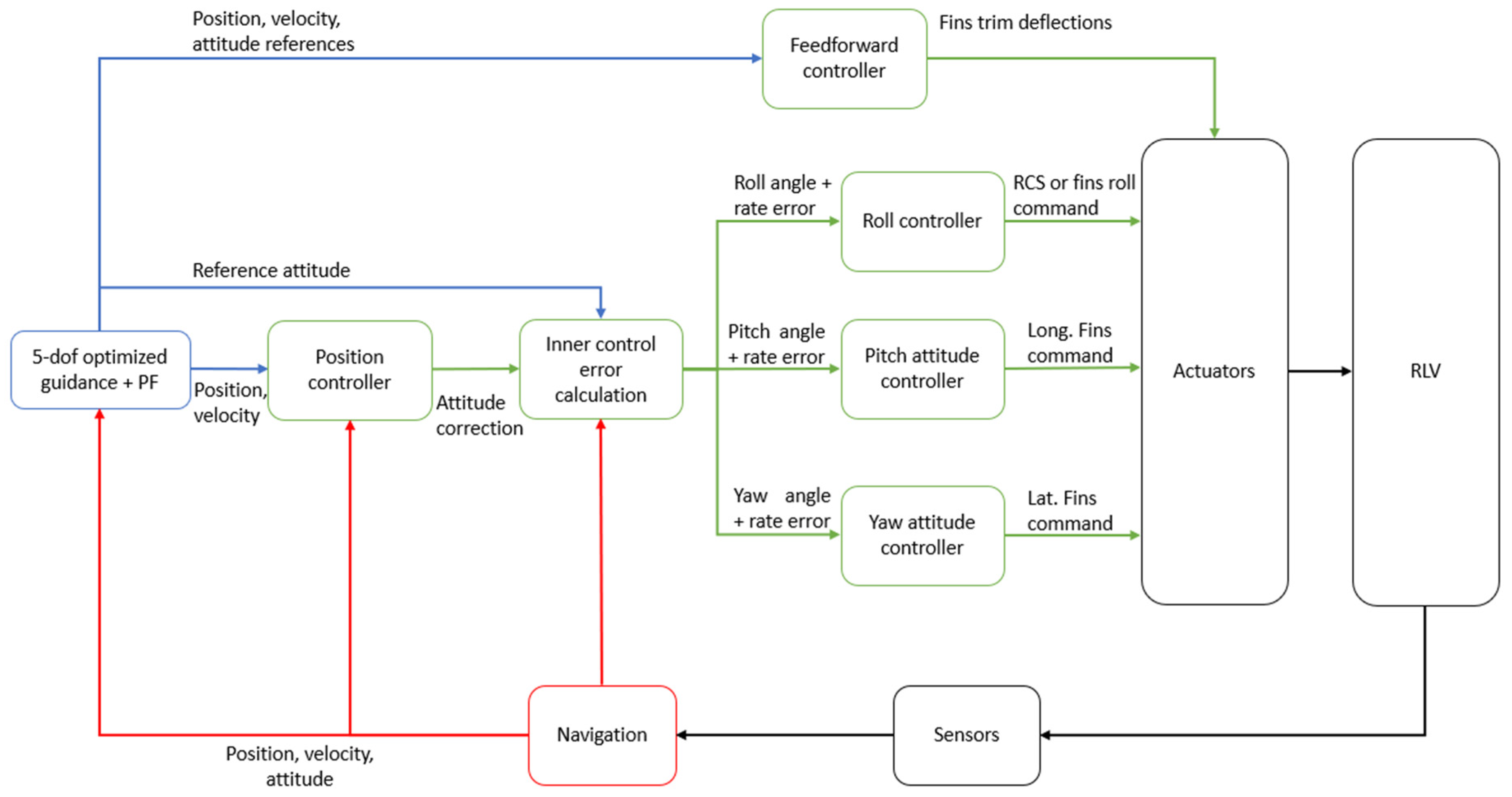
3.1. GNC Functional Architecture

Figure 2 shows the functional architecture of the GNC solution proposed for the return mission of first stage of a launcher.

The GNC solution comprises the following algorithms:

• Flight Management (FM): The FM oversees both the internal status and data from all the other functions and defines the functional modes of each of them depending on the phase and the conditions of flight. The FM interacts with the Mission Vehicle Management (MVM), which manages the interaction of the GNC with other vehicles subsystems.
• Guidance: The objective of the guidance algorithm is to define the reference trajectory and the control actions required to track it. This shall be designed so as to allow for the vehicle to arrive at the designated target site, satisfying the mission and flight path constraints.
• Navigation: The navigation function estimates the current state of the system. The navigation solution is served primarily by the inertial measurement unit (IMU or INS (inertial navigation system)), which is hybridized with a (D)GNSS receiver. Navigation could also make use of other sensors (e.g., FADS (Flush Airdata Sensing), altimeter), if available, depending on the mission phase, even if they are not strictly required.
• Control: The control function task is to ensure a correct tracking of the reference states generated by the guidance using the GNC’s available actuators.

The control and navigation functions interact with the actuators and sensors. The FM function collects status information and data from each of the GNC system main functions and further sends them to the MVM, which, based on the information received from the ground function and from the other vehicle subsystems, sends back updated information to the FM function. As mentioned above, the FM function uses the updated data to define the appropriate functional mode for each of the guidance, navigation, and control functions.

3.2. GNC Modes

This section describes the modes of operation for the GNC solution developed in the framework of SALTO for the DRL presented in Section 2. They are defined by the mission phase, and are the following:

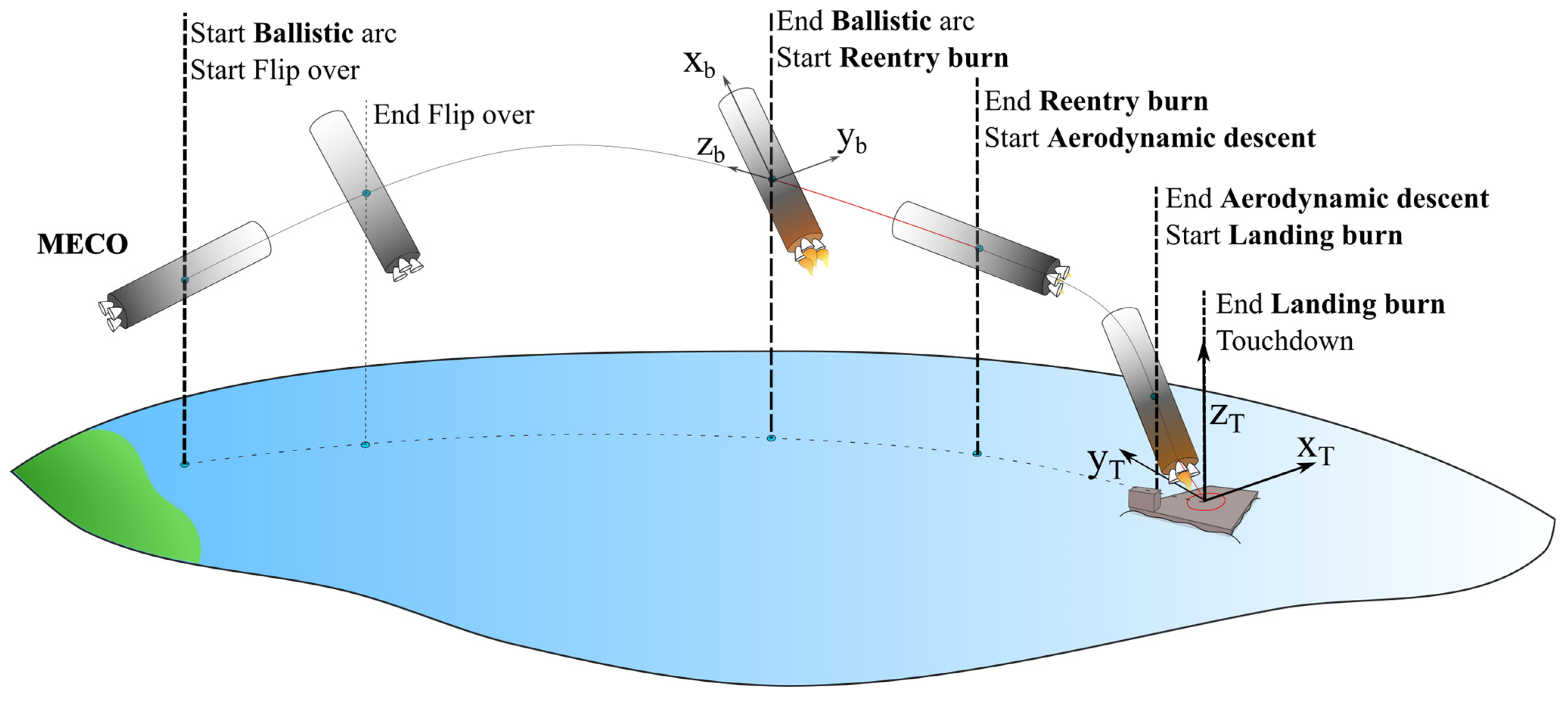
• High-altitude ballistic flight: During this phase, neither thrust nor aerodynamic forces are available to perform trajectory control. The control function actuates the RCS to perform a flip-over and aligns the vehicle to the reference attitude for the re-entry burn. During this phase, the aerodynamic control surfaces (ACSs) are deployed. The navigation function continues estimating the position, velocity, and attitude, making use of inertial measurements fused with (D)GNSS updates.
• Re-entry burn: During the re-entry burn, the vehicle carries out a retro-propulsion braking maneuver to reduce the velocity of the booster and limit the aerodynamic load. When this mode is triggered, the guidance function generates a trajectory (position, velocity, attitude, and throttle profile) accounting for the vehicle’s initial conditions and operational constraints, and the control function takes care of orienting and steering the vehicle using the TVC, RCS, and throttle modulation (the effectiveness of the ACS is too low during this phase). The navigation function continues estimating the position, velocity, and attitude, making use of inertial measurements fused with (D)GNSS updates.
• Aerodynamic phase: During the aerodynamic phase, the guidance function outputs a reference trajectory to target the correct location at the start of the landing burn by modulating the attitude. The control function uses fins and RCS to correct the vehicle drift with respect to the guidance reference. The navigation function continues estimating the position, velocity, and attitude, making use of inertial measurements fused with (D)GNSS updates and with (F)ADS measurements, if available.
• Landing burn: During the landing phase, the guidance function commands the nominal throttle profile and thrust orientation required to perform a safe approach to the recovery barge and achieve pinpoint landing. The control function uses the TVC, ACS, RCS, and throttle modulation to perform the required maneuvers and track the desired path. The navigation function could use an altimeter and (F)ADS, if available, to further improve the accuracy of the estimation approaching the landing site.

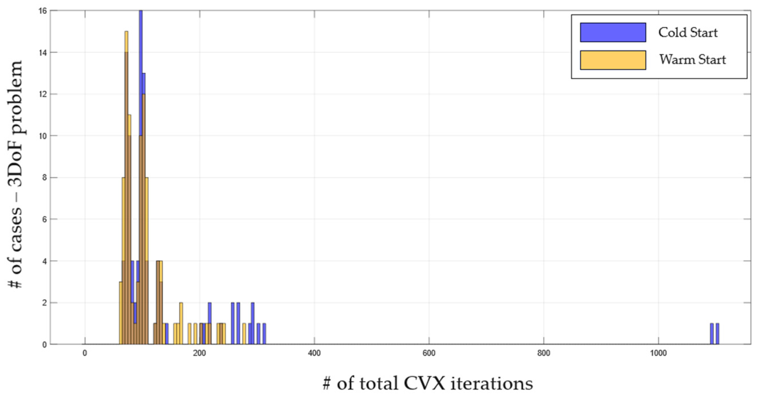
3.3. Sequential Convex Programming (SCP) Onboard Guidance

The guidance strategy presented in this work adopts a real-time implementation of the SCP algorithm. In recent years, this algorithm has been widely used to solve generic non-convex optimal control problems of the following form:

$$\begin{array}{cc}\underset{x, u,p}{\mathrm{m}\mathrm{i}\mathrm{n}\mathrm{i}\mathrm{m}\mathrm{i}\mathrm{z}\mathrm{e}}& J(\mathit{x}\left(t\right),\mathit{u}\left(t\right),\mathit{p})\\ & \\ \mathrm{s}\mathrm{u}\mathrm{b}\mathrm{j}\mathrm{e}\mathrm{c}\mathrm{t} \mathrm{t}\mathrm{o}:& \dot{\mathit{x}}\left(t\right)=\mathit{f}(\mathit{x}\left(t\right),\mathit{u}\left(t\right),\mathit{p})\\ & A_0\mathit{x}\left(t_0\right)={\mathit{x}}_0\\ & A_f\mathit{x}\left(t_f\right)={\mathit{x}}_{\mathit{f}}\\ & \mathit{g}\left(\mathit{x}\left(t\right),\mathit{u}\left(t\right),\mathit{p}\right)\le 0\end{array}$$

(1)

where $\mathit{x}\left(t\right)\in {\mathbb{R}}^{n_x}$ is the state vector, $\mathit{u}\left(t\right)\in {\mathbb{R}}^{n_u}$ is the control input vector, and $\mathit{p}\in {\mathbb{R}}^{n_p}$ is the parameters vector. Note that if the optimal control problem is a free final time problem, it can be formulated in the form of (1) by exploiting the parameter vector $\mathit{p}$. The system of functions $\mathit{f} :{\mathbb{R}}^{n_x}\times {\mathbb{R}}^{n_u}\times {\mathbb{R}}^{n_p}\to {\mathbb{R}}^{n_x}$ represents the set of dynamics constraints, while $A_0$ and $A_f$ are used to impose the boundary conditions by defining the subset of the state vector constrained at the initial and final time. The function $\mathit{g} :{\mathbb{R}}^{n_x}\times {\mathbb{R}}^{n_u}\times {\mathbb{R}}^{n_p}\to {\mathbb{R}}^{n_c}$ describes the set of equality and inequality path constraints. $\mathit{g}$ also includes the bounds on the optimization variables if needed. Lastly, $J :{\mathbb{R}}^{n_x}\times {\mathbb{R}}^{n_u}\times {\mathbb{R}}^{n_p}\to \mathbb{R}$ is the cost function, such that it can be constituted by both the Mayer and Lagrange terms.

The SCP algorithm iteratively solves the problem in (1) after transforming it into a Second-Order Cone Programming (SOCP) problem. To obtain the SOCP, the original problem is convexified with a First-Order Taylor expansion of the non-convex terms about the current reference solution (starting from an initial guess) and by involving virtual controls, dynamics relaxations, and trust regions to avoid artificial infeasibility and artificial unboundedness [7]. These terms drive the convergence, so they are monitored along the solving routine and define the stopping criteria of the algorithm. The convex approximation is used to formulate an SOCP in the following standard conic form:

$$\begin{array}{cc}\underset{z}{\mathrm{m}\mathrm{i}\mathrm{n}\mathrm{i}\mathrm{m}\mathrm{i}\mathrm{z}\mathrm{e}}& {\mathit{c}}^T\mathit{z}\\ & \\ \mathrm{s}\mathrm{u}\mathrm{b}\mathrm{j}\mathrm{e}\mathrm{c}\mathrm{t} \mathrm{t}\mathrm{o}:& A\mathit{z}=\mathit{b}\\ & G\mathit{z}+\mathit{s}=\mathit{h}, \mathit{s}\in \mathcal{K}\\ & \end{array}$$

(2)

where $\mathit{z}\in {\mathbb{R}}^{n_z}$ are the primal variables, $\mathit{s}$ denotes slack variables, while $\mathit{c}\in {\mathbb{R}}^z$, $A\in {\mathbb{R}}^{n_{ceq}\times n_z}$, $\mathit{b}\in {\mathbb{R}}^{n_{ceq}},$ $G\in {\mathbb{R}}^{n_{cineq}\times n_z}$, and $\mathit{h}\in {\mathbb{R}}^{n_{cineq}}$ are the problem data. $\mathcal{K}=C_L\times C_{Q_1}\times \dots \times C_{Q_m}$ is the cone such that the first $l\ge 0$ cones correspond to the positive orthant $C_L=\left\{\mathit{w}\in {\mathbb{R}}^l\right|\mathit{w}\ge 0\}$, and each $C_{Q_i}=\left\{({\mathit{w}}_0,\mathit{w})\in {\mathbb{R}}^{q_i}\right|{\left|\left|\mathit{w}\right|\right|}_2\le {\mathit{w}}_0\}$. Once the problem defined in (2) is solved, a new reference trajectory is available to convexify (1) and move to the next SCP iteration; this process is repeated until the convergence criteria are met.

In this work, the SCP algorithm is applied to three different optimal control problem formulations to obtain onboard an optimal reference trajectory at the beginning of the powered re-entry, the aerodynamic descent, and the powered landing phases. This strategy aims at coping with the accumulated tracking errors along the descent and fulfilling the strict pinpoint landing requirements. The guidance is fed by a set of waypoints (one for each phase) obtained within mission analysis; each waypoint defines the conditions at which the phase change should happen. As waypoints cannot be exactly matched by the GNC, the flight manager commands the mode change when the target altitude is reached. A different and adaptive logic is used to move from ballistic mode to re-entry, as detailed in Section 4.1.1.

3.4. Real-Time Implementation and PIL Integration

Typically, successive convexification and sequential convex programming approaches have relied on modeling interfaces, often referred to as parsers, to automate the conversion of the optimization process in the SOCP structure (2). While these parsers simplify problem formulation, they introduce several drawbacks, including computation overhead, redundant constraints, and dynamically allocated memory. These limitations are particularly problematic for real-time spaceflight applications, where efficiency and reliability are critical [24].

In the next subsection, the methodology followed in this work is presented. It relies on an “Offline pre-parser” and an “Online parser”. The offline pre-parser builds the structure of the problem depending on the original problem formulation and the user design choices, while the online parser exploits the obtained problem structure and only manipulates those elements that depend on the flight conditions and on the sequential convex iteration without modifying the problem structure. The objective is to reduce at the minimum the operations performed by the online module.

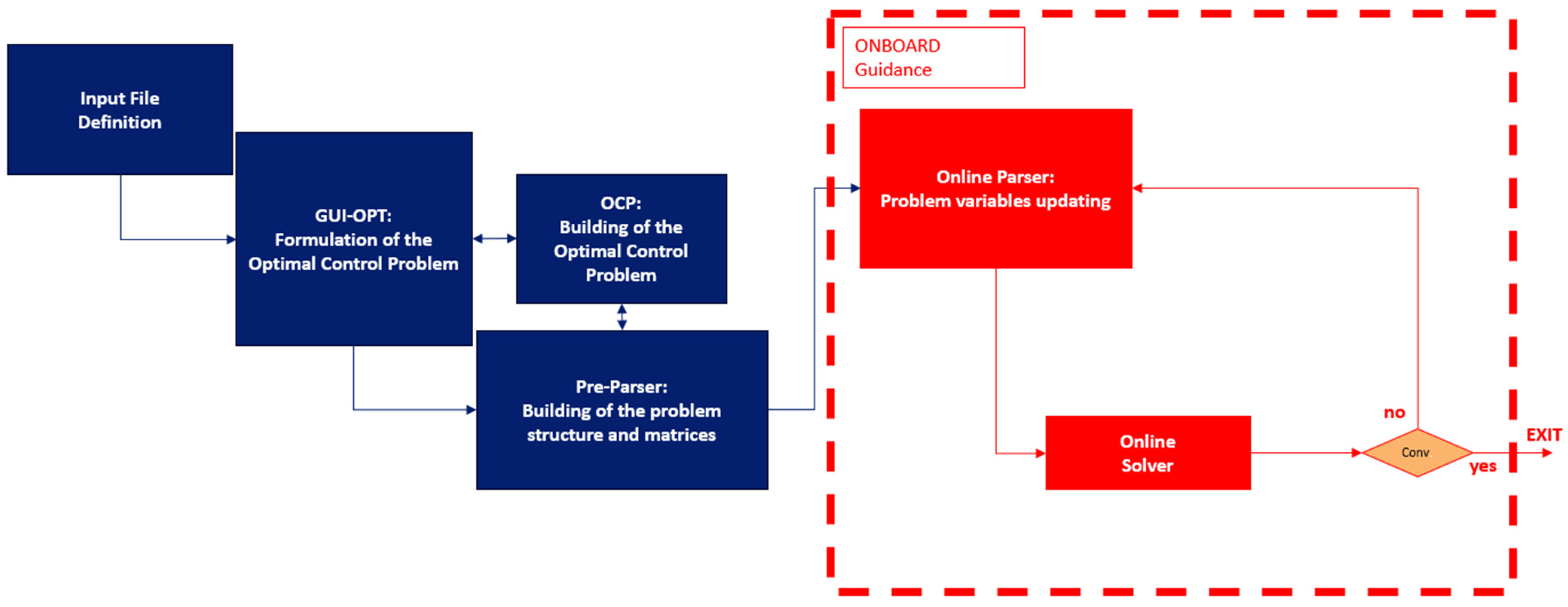
3.4.1. Offline Pre-Parsing

The pre-parsing consists of initializing the matrices A, b, G, and h used in (2). To achieve this operation, the pre-parser interfaces with Deimos proprietary tools (Gui-opt and OCP blocks in Figure 3) that can be used to define the problem depending on its formulation and the user assumptions. Figure 3 shows a block diagram with the operation performed by the offline pre-parser, the interfacing tool, and an emulator of the onboard software. Once the problem is built, the formulation and structure of the problem can be considered fixed, and it does not change along the SCP iterations. A paramount action performed by the pre-parser is the identification of both the non-zero entries and the non-zero entries that must be updated during the sequential convexification and during the flight. In other words, the pre-parse must compute the sparsity pattern of A, b, G, and h. Concerning the constant non-zero elements, the pre-parser simply populates the matrices with the problem-dependent constants, while for the non-constant non-zero elements, the pre-parser initializes the values by exploiting the provided initial guess and identifies their positions in the matrices such that the online parser can update them.

To accomplish this process, an enumeration of the variables and constraints must be defined. In this paper, the enumeration for each phase is reported in the dedicated section.

3.4.2. Online Parsing and Solving

The onboard software is constituted by the online parser and the solver. The online parser exploits all the information computed by the offline parser to update the non-constant elements; it replaces the updated variables into the right positions of the matrices, thanks to the problem structure information computed offline. This allows for avoiding computational overheads, redundant operations that can be performed only once, and dynamically allocated memory.

The updating of the non-constant elements depends on the variables themselves. The terms that change due to the convexification of the problem are the most critical ones, since the re-evaluation of the linearized model must be carried out around the new updated solution computed by the solver. This operation is performed by evaluating a set of functions that have been calculated offline through CasADi [25]. These functions define the Jacobians of the nonlinear constraints with respect to the state, the control, and the final time. Other elements, such as the flight conditions and the trust region radius, are simply replaced without further operations. This machinery allows for updating the non-constant values of the sparsity pattern without performing a complete parsing at each iteration of the SCP. The updated problem is then provided to the solver, which solves it till the convergence criteria of the SCP are met. The obtained solution constitutes the reference commands that must be tracked by the controller. In this context, an in-house solver for conic optimization has been developed with similar features to ECOS [26].

The computational efficiency of such guidance strategy is a crucial aspect; for this reason, future works foresee dedicated analysis on the computational burden of GNC solutions. This work does not report any results in terms of computational efficiency, as the results presented were obtained with MIL (model-in-the-loop) simulations. The computational performance observed in MIL, which are very promising, may not accurately reflect real-world performance, particularly when considering the execution of these algorithms onboard a reusable rocket. Onboard execution, indeed, involves additional complexities, as it requires comprehensive integration and optimization of both software and hardware systems. These developments and analysis in PIL (processor-in-the-loop) are currently under investigation and are foreseen for future steps of the project.

3.5. Control Methods Overview

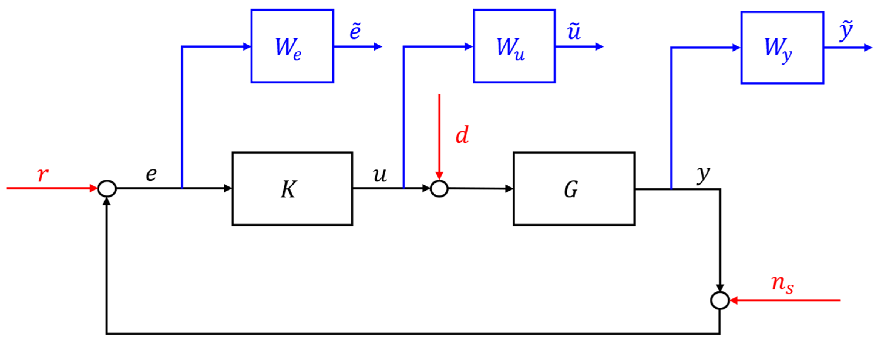
3.5.1. Control Problem Formulation

The control logic makes use of linear controllers synthesized with structured H-infinity robust control methods [27]. The control synthesis problem setup is shown in Figure 4, where black components highlight the linearized plant dynamics (see Section 3.5.2) to be controlled and the controller to be synthesized; in blue, the dynamic weights shaping the closed loop response are represented. These weighs are used to specify the desired closed-loop performance according to the H-infinity formalism. Red arrows represent the exogenous input signals, i.e., reference, disturbance, and noise. A description of the components can be found in

Table 3. List of elements for loop shaping.

Elements	Description
$\mathit{r}$	Reference signal to be tracked when closing the loop
$\mathit{e}$	Control error
$\tilde{\mathit{e}}$	Filtered control error
$\mathit{u}$	Controller output (plant input)
$\tilde{\mathit{u}}$	Filtered control output
$\mathit{d}$	Plant disturbance
$\mathit{y}$	Measurement (or estimate) available for control
$\tilde{\mathit{y}}$	Filtered measurement
${\mathit{n}}_{\mathit{s}}$	Measurement noise
$\mathit{K}$	Controller
$\mathit{G}$	Plant (linearized)
${\mathit{W}}_{\mathit{e}}$	Weight on control error
${\mathit{W}}_{\mathit{u}}$	Weight on control signal
${\mathit{W}}_{\mathit{y}}$	Weight on measurement
$\mathit{K}$	Controller

.

The synthesis problem is formulated as a structured multi-objective optimization problem of the following form [28]:

$$\begin{array}{cc}\mathrm{m}\mathrm{i}\mathrm{n}\mathrm{i}\mathrm{m}\mathrm{i}\mathrm{z}\mathrm{e}& \max (Re{q}_1, \dots , Re{q}_n)\\ K& \\ \mathrm{s}\mathrm{u}\mathrm{b}\mathrm{j}\mathrm{e}\mathrm{c}\mathrm{t} \mathrm{t}\mathrm{o}:& K\in K_{set}\\ & K stabilizing\end{array}$$

(3)

where the requirements are in general expressed as the H-infinity norm of some specified closed-loop input–output channels; the controller $K$ must stabilize the closed loop and it is constrained to the set of controllers with a predefined structure; in the context of this project, the controller structures are explained in Section 4.

By denoting $T_{ij}$ as the closed loop transfer function from input $i$ to output $j$, it is common to formulate a requirement as

$$Re{q}_h={‖W_h{T}_{ij}‖}_{\infty }$$

(4)

where $W_h$ denotes a suitable proper filter. It is worth noting that for a SISO system, the H-infinity norm is given by the peak of the magnitude of the frequency response function. This stated, it is common to select the filter $W_h$ such that it shapes the desired response of the selected input–output pair.

A list of control objectives for the controller synthesis is summarized in Table 4. In the left column, the high-level objective is specified; in the right column, the corresponding synthesis requirement can be found. In this sense, we consider the following high-level control objectives:

• Setpoint tracking: Of paramount importance to ensure good accuracy in terms of either position or attitude reference profile tracking.
• Disturbance attenuation: The control system must be capable of rejecting external perturbations.
• Control effort moderation: The control system actuators present a physical limitation. This limitation must be accounted for during the tuning process.
• Stability margins: It is of paramount importance that the closed loop is stable in presence of unmodelled effects and parametric uncertainties. Robustness can be quantified via classical gain and phase margins or disk margins.

Table 4. List of control objectives used in multi-objective tuning approach.

High Level Objective	Synthesis Objective
Setpoint tracking	$\mathrm{Optimization} \mathrm{of} \mathrm{transfer} \mathrm{function} T_{r\tilde{e}}$
Disturbance attenuation	$\mathrm{Optimization} \mathrm{of} \mathrm{transfer} \mathrm{function} T_{d\tilde{y}}$
Control effort moderation	$\mathrm{Optimization} \mathrm{of} \mathrm{transfer} \mathrm{function} T_{r\tilde{u}}$
Stability margins at input	$\mathrm{Ensuring} \mathrm{disk} \mathrm{margin} \mathrm{at} \mathrm{loop} \mathrm{break} \mathrm{pair} d,u$
Stability margins at output	$\mathrm{Ensuring} \mathrm{disk} \mathrm{margin} \mathrm{at} \mathrm{loop} \mathrm{break} \mathrm{pair} y,n$
Setpoint tracking	$\mathrm{Optimization} \mathrm{of} \mathrm{transfer} \mathrm{function} T_{r\tilde{e}}$

Table 4. List of control objectives used in multi-objective tuning approach.

High Level Objective	Synthesis Objective
Setpoint tracking	$\mathrm{Optimization} \mathrm{of} \mathrm{transfer} \mathrm{function} T_{r\tilde{e}}$
Disturbance attenuation	$\mathrm{Optimization} \mathrm{of} \mathrm{transfer} \mathrm{function} T_{d\tilde{y}}$
Control effort moderation	$\mathrm{Optimization} \mathrm{of} \mathrm{transfer} \mathrm{function} T_{r\tilde{u}}$
Stability margins at input	$\mathrm{Ensuring} \mathrm{disk} \mathrm{margin} \mathrm{at} \mathrm{loop} \mathrm{break} \mathrm{pair} d,u$
Stability margins at output	$\mathrm{Ensuring} \mathrm{disk} \mathrm{margin} \mathrm{at} \mathrm{loop} \mathrm{break} \mathrm{pair} y,n$
Setpoint tracking	$\mathrm{Optimization} \mathrm{of} \mathrm{transfer} \mathrm{function} T_{r\tilde{e}}$

As the controller is structured, the $H_{\infty }$ problem in (3) is non-convex and convergence to a global minimum cannot be ensured [28]. The problem can be efficiently solved through optimization algorithms available in the MATLAB 2022a robust control toolbox.

Moreover, as the open-loop properties of the plant vary along the trajectory, the controller gains are scheduled with the airspeed. Smoothness of the global controller is ensured by appropriately starting the optimization of each local controller with a suitable guess (i.e., the solution at the previous scheduling point).

Linear analysis tools can be used then to assess the robustness properties of the designed controller along the trajectory as shown in, e.g., [20,21,29]. The specific results are omitted in the scope of this paper but can be found in [21,30].

3.5.2. Control-Oriented Modelling

The purpose of this section is to describe the control-oriented models needed to define and tune the control logic. Linear models are used, as they provide a very good description of the fundamental effects and critical aspects of involved in the dynamics of a launch vehicle. As is common in the launcher control community, a decoupled design is considered for pitch/yaw, and it exploits the vehicle’s axial symmetric properties. The roll channel is analyzed independently of those two. Special care is also taken for the axial dynamics; this is something that is not usually considered during the ascent phase, but it is of paramount importance for the descent, as appropriate control of the vehicle’s speed is needed. Engine throttling is used for this purpose.

Concerning the pitch (the equivalent consideration applies for yaw) channel, the following linearized time invariant control-oriented model is considered:

$$\left[\begin{array}{c}\dot{\theta }\\ \dot{q}\\ \dot{w}\end{array}\right]=\left[\begin{array}{ccc}0& 1& 0\\ 0& 0& {\displaystyle \frac{{\mu }_{\alpha }^{\prime }}{u_0}}\\ -a_0& u_0& -{\displaystyle \frac{N_{\alpha }^{\prime }}{m{u}_0}}\end{array}\right]\left[\begin{array}{c}\theta \\ q\\ w\end{array}\right]+\left[\begin{array}{ccc}0& 0& 0\\ -{\mu }_c& {\mu }_f& -{\displaystyle \frac{l_f}{J}}\\ -{\displaystyle \frac{T}{m}}& -{\displaystyle \frac{N_f}{m}}& {\displaystyle \frac{1}{m}}\end{array}\right]\left[\begin{array}{c}{\beta }_{\theta }\\ {\delta }_{f,\theta }\\ F_Z\end{array}\right],$$

(5)

where the terms in (5) can be found in [31]. It is worth noting that this model is completely generic, and it is used for the different mission phases. The linear kinematics for the control of the lateral drift with respect to the reference trajectory yields are as follows:

$$\left[\begin{array}{c}\dot{x}\\ \dot{y}\\ \dot{z}\end{array}\right]=\left[\begin{array}{c}u\\ v+\psi u_0\\ w-\theta u_0\end{array}\right].$$

(6)

with $u, v,$ and $w$ denoting the components of the velocity in body frame. Concerning the roll channel, the following approximation of the rigid roll mode is considered:

$$\left[\begin{array}{c}\dot{\varphi }\\ \dot{p}\end{array}\right]=\left[\begin{array}{cc}0& 1\\ 0& 0\end{array}\right]\left[\begin{array}{c}\varphi \\ p\end{array}\right]+\left[\begin{array}{c}0\\ {\displaystyle \frac{1}{J_{xx}}}\end{array}\right]M_x,$$

(7)

with $M_x$ defining the roll control torque and $J_{xx}$ the roll inertia moment.

For the axial dynamics, assuming that the vehicle is flying close to a zero-lift condition, we get

$$\dot{V}\approx {\displaystyle \frac{2D_0}{m{V}_0}}V+{\displaystyle \frac{T}{m}}{T}_h,$$

(8)

where $D_0, { T}_0$ are the reference drag and thrust, respectively, $V$ is the flight speed, and $T_h$ denotes the throttle variation.

4. Guidance and Control Design

This section presents the G&C strategies and methodologies developed in each mission phase of the recovery of the first stage.

4.1. Flip-Over and Ballistic Phase

The goal of the G&C for this phase is to reorient the vehicle to an attitude which enables a correct firing of the engine at the beginning of the re-entry phase. This operation is done by following two steps: firstly, the final attitude to be reached is computed online through the aid of Lookup Tables (LUTs) according to the scheduling logic obtained offline, then a smooth guidance law is generated to orient the vehicle from the initial attitude at MECO to the final target attitude during the flip-over. Once the final attitude is achieved, it is kept constant till the re-entry burn phase starts. The LUTs, used to schedule the final attitude, also provide the ignition height to start the re-entry burn, which is exploited within the FM for the phase management. The scheduling LUTs were developed by following a similar methodology reported in [23], and it is briefly explained hereafter.

4.1.1. Scheduling LUT

Considering nominal MECO conditions, a specific ignition height and attitude optimize fuel consumption during the re-entry burn to target the desired aerodynamic descent initial conditions. However, dispersed MECO conditions determine errors in downrange and crossrange for which nominal ignition height and attitude may lead to unfeasible powered trajectories. Therefore, an adaptation of the ignition height and attitude to MECO conditions is required to target the initial condition of the aerodynamic phase. To address this problem, a set of LUTs are computed offline by optimizing the ignition height and attitude given a discrete number of MECO conditions. The LUTs are then used online by the onboard software. In particular, these are built by considering $\pm 3\sigma$ dispersed values in groundspeed $v_{MECO}$, heading angle ${\chi }_{MECO}$, and combined cases. The dispersions on these variables, indeed, generate the largest errors at the re-entry burn interface. The computation of the optimal ignition height and attitude is performed by following the procedure illustrated in Figure 5. Firstly, for each MECO condition, a ballistic trajectory is obtained. Then, a family of pure 3DoF free final time Powered Descent Guidance (PDG) problems is solved by means of direct optimization methods by varying the initial height. IPOPT is used as the NLP solver for this step [32]. While an indirect method is used in [23] to privilege optimality, here, a direct method is used, as it allows for an easier generalization of the problem to different types of dynamics and constraints. The computation starts from the highest altitude, and then it is reduced till infeasibility is detected. The optimization problems are initialized with a warm guess exploiting a continuation method. Such continuation heuristic, common to indirect optimization [33], and has recently proven useful for direct methods as well [34]. In this way, a feasible ignition height vector is obtained for each MECO condition. From this vector, the optimal ignition altitude is selected, and a 5DoF Angle-of-Attack constrained free final time PDG problem [13] is solved by exploiting the SCP approach (Section 3.3), letting the initial attitude be unconstrained and considering it as an optimization variable. For this last step, the same SCP algorithm run by the guidance is used to refine the values of the LUTs; this helps in reducing the difference between the predicted offline values and the ones generated onboard in presence of dispersions in the initial states of the vehicle. If such an optimization problem does not converge by considering the optimal ignition height, a suboptimal higher altitude is used as the initial condition for the optimization since a feasible solution is found. This procedure yields to a set of feasible fuel-optimal ignition height and altitude, which depends on the MECO conditions, that can be exploited online.

4.1.2. Slew Maneuver Design

Concerning the commanded attitude logic to perform the flip-over, it is assumed that the time necessary for the maneuver is fixed. An optimal time for the maneuver can be found offline when the RCSs are sized; for a downrange landing scenario the flip-over time is not a relevant issue. The rotation law for the flip-over is defined as

$$R_g\left(t\right)=\Delta R\left(t\right)R_0$$

(9)

with boundary conditions given by $\Delta R\left(t_f\right)=R_f{R}_0^T$ and $\Delta R\left(t_0\right)=I_3$.

The definition of $\Delta R\left(t\right)$ exploits the axis-angle parametrization, which can be expressed as follows [35] (pp. 17–65):

$$\Theta =\mathrm{acos}\left({\displaystyle \frac{1}{2}}\left(tr\left(R\right)-1\right)\right),$$

(10)

$$\widehat{\mathit{n}}={\displaystyle \frac{1}{2sin\Theta }}\left[\begin{array}{c}{R}_{32}^T-R_{23}^T\\ R_{13}^T-R_{31}^T\\ R_{21}^T-R_{12}^T\end{array}\right],$$

(11)

with the corresponding description for the rotation matrix:

$$R^T=\left[\begin{array}{ccc}{\widehat{\mathit{n}}}^2\left(1\right)(1-\cos \Theta )+\cos \Theta & \widehat{\mathit{n}}\left(1\right)\widehat{\mathit{n}}\left(2\right)(1-\cos \Theta )-\widehat{\mathit{n}}(3)\sin \Theta & \widehat{\mathit{n}}\left(1\right)\widehat{\mathit{n}}\left(3\right)(1-\cos \Theta )+\widehat{\mathit{n}}(2)\sin \Theta \\ \widehat{\mathit{n}}\left(1\right)\widehat{\mathit{n}}\left(2\right)(1-\cos \Theta )+\widehat{\mathit{n}}(3)\sin \Theta & {\widehat{\mathit{n}}}^2\left(2\right)(1-\cos \Theta )+\cos \Theta & \widehat{\mathit{n}}\left(2\right)\widehat{\mathit{n}}\left(3\right)(1-\cos \Theta )-\widehat{\mathit{n}}(2)\sin \Theta \\ \widehat{\mathit{n}}\left(1\right)\widehat{\mathit{n}}\left(3\right)(1-\cos \Theta )-\widehat{\mathit{n}}(2)\sin \Theta & \widehat{\mathit{n}}\left(2\right)\widehat{\mathit{n}}\left(3\right)(1-\cos \Theta )+\widehat{\mathit{n}}(2)\sin \Theta & {\widehat{\mathit{n}}}^2\left(3\right)(1-\cos \Theta )+\cos \Theta \end{array}\right].$$

(12)

The idea is to define an attitude law for $\Delta R\left(t\right)$ exploiting the axis-angle parametrization. In particular, the rotation vector is known by (11) and $\Delta R\left(t_f\right).$ The law for the angle parameter $\Theta$ is defined using a trapezoidal profile for its time derivative and considering the known boundary conditions for (9).

4.1.3. Flip-Over Control Design

At such high altitudes, the contribution of the aerodynamic forces is negligible, and the control design neglects the effect of these perturbations; RCSs are used for the generation of the necessary torque to keep the vehicle orientation. For this phase, only the rotational equation is considered. The effect of the RCS controls on the translational equation is negligible with respect to the gravitational pull of the Earth. The Euler rotational equation is given by

$$J\dot{\mathit{\omega }}+\mathit{\omega }\times J\mathit{\omega }={\mathit{M}}_{RCS}$$

(13)

and given the axial symmetric properties of the vehicle, the different channels and axes are decoupled. The control action makes use of a feedforward and a feedback part. The former is given by

$${\mathit{M}}_{ff}=\widehat{J}{\dot{\mathit{\omega }}}_g+{\mathit{\omega }}_g\times \widehat{J}{\mathit{\omega }}_g$$

(14)

where $\widehat{J}\in {\mathbb{R}}^{3\times 3}$ is the nominal value of the inertia tensor and ${\mathit{\omega }}_g\in {\mathbb{R}}^3$ is the velocity generated by the flip-over guidance; the latter is given by a PD control law, which yields

$$F_Z=k_{p,\theta }{\theta }_e+k_{d,\theta }{q}_e$$

(15)

$$F_Y=k_{p,\psi }{\psi }_e+k_{d,\psi }{r}_e$$

(16)

$$M_X=k_{p,\varphi }{\varphi }_e+k_{d,\varphi }{p}_e$$

(17)

for pitch, yaw, and roll channels, respectively. Please note that pitch and yaw controllers directly command the total force demanded to the RCS cluster. A control allocation function manages the thrusters firing according to their disposition on the vehicle. The rotation error is defined as the Euler angle sequence parametrizing the rotation error in matrix form $R_e$ as

$$R_e=R_n{R}_g^T,$$

(18)

where $R_n, R_g$ denote the estimated attitude by the navigation function and the commanded attitude, respectively. The angular rate error ${\mathit{\omega }}_e\in {\mathbb{R}}^3$ is defined as

$${\mathit{\omega }}_e={\mathit{\omega }}_n-{\mathit{\omega }}_g.$$

(19)

The controllers are tuned using a structured H-infinity approach as discussed in Section 4.1.3.

4.2. Re-Entry Burn Phase

The aims of the G&C during the re-entry phase are to reduce the velocity of the rocket while targeting the desired initial conditions of the aerodynamic descent. This phase is crucial, since most of the position error accumulated during the ballistic phase is compensated here. This goal is achieved by performing a retro-propulsive maneuver.

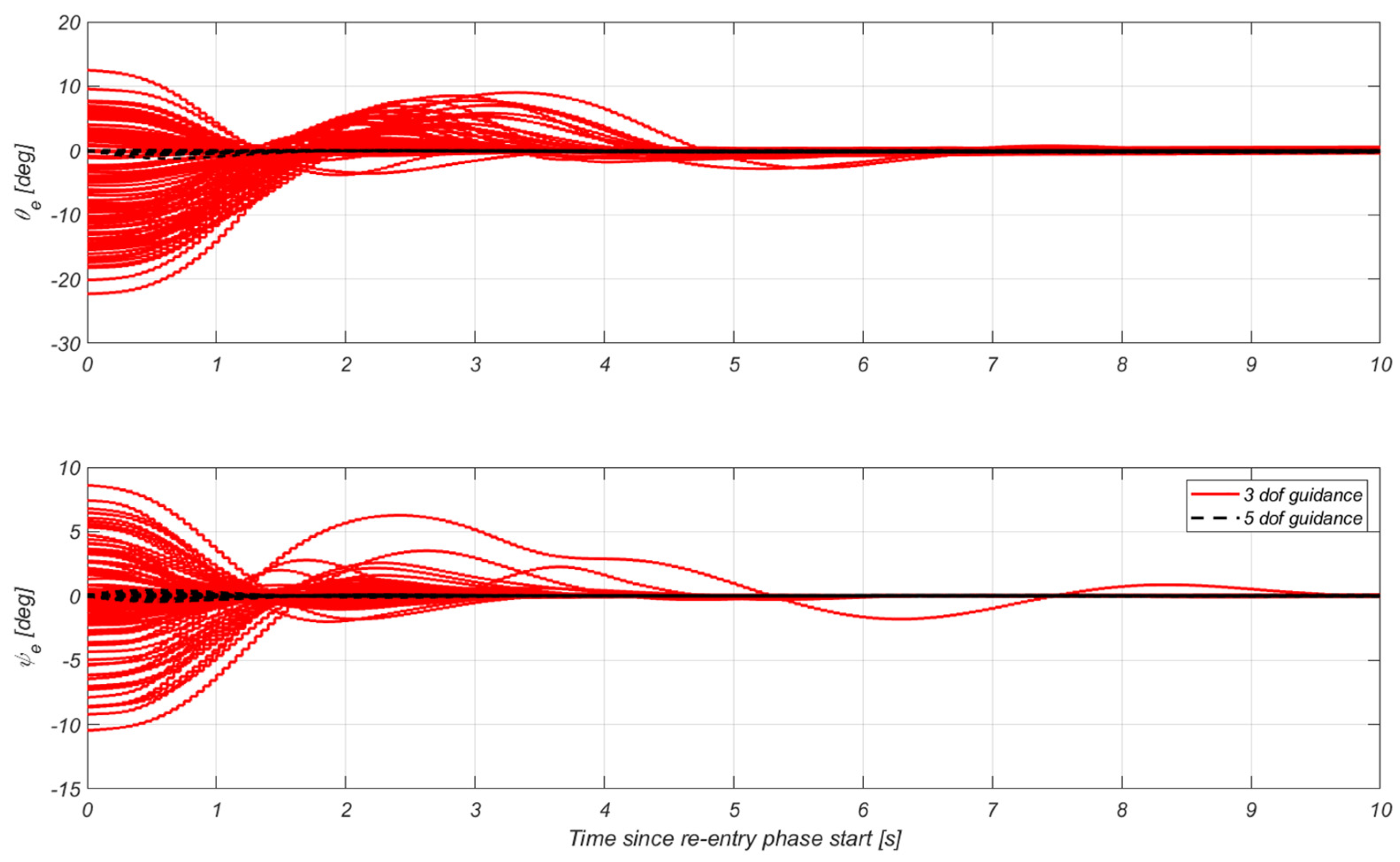
4.2.1. Powered Re-Entry Guidance Design

The guidance solves the 5DoF free final time fuel-optimal powered pinpoint re-entry problem to generate a reference trajectory that the control must track. The problem is formulated in an East–North–Up (ENU) reference frame centered at the landing point. In this phase, the optimization problem is formulated as follows:

$$\begin{array}{cc}\underset{\mathit{u}, t_f}{\mathrm{m}\mathrm{i}\mathrm{n}\mathrm{i}\mathrm{m}\mathrm{i}\mathrm{z}\mathrm{e}}& J_{rnt}=w_T{{\displaystyle \int }}_0^{t_f}Tdt+w_u{{\displaystyle \int }}_0^{t_f}\left(u_{\psi }^2+u_{\theta }^2\right)dt\\ & \\ \mathrm{s}\mathrm{u}\mathrm{b}\mathrm{j}\mathrm{e}\mathrm{c}\mathrm{t} \mathrm{t}\mathrm{o}:& \dot{\mathit{x}}\left(t\right)={\mathit{f}}_{\mathit{r}\mathit{n}\mathit{t}}(\mathit{x}\left(t\right),\mathit{u}\left(t\right))\\ & {\mathit{r}}_0={\overline{\mathit{r}}}_0, {\mathit{v}}_0={\overline{\mathit{v}}}_0,m_0={\overline{m}}_0, {\psi }_0={\overline{\psi }}_0, {\theta }_0={\overline{\theta }}_0 \\ & {\mathit{r}}_f=\overline{{\mathit{r}}_f}, {\mathit{v}}_f={\overline{\mathit{v}}}_f, {\psi }_f={\overline{\psi }}_f, {\theta }_f={\overline{\theta }}_f\\ & T_{min }\le T\le T_{max} \\ & \left|u_{\psi }\right|\le u_{ \psi ,max}, \left|u_{\theta }\right|\le u_{ \theta ,max}, \left|u_T\right|\le u_{ T,max}\\ & \left|{\dot{u}}_{\psi }\right|\le {\dot{u}}_{ \psi ,max}, \left|{\dot{u}}_{\theta }\right|\le {\dot{u}}_{ \theta ,max}\end{array}$$

(Problem 1)

where the state $\mathit{x}={\left[{\mathit{r}}^T,{\mathit{v}}^T,m,\psi ,\theta ,T\right]}^T\in {\mathbb{R}}^{10}$ includes the position, velocity, mass, yaw and pitch angles, and thrust magnitude, respectively. The control vector $\mathit{u}={\left[u_{\psi }, u_{\theta }, u_T\right]}^T\in {\mathbb{R}}^3$ gathers the commanded yaw rate, pitch rate, and thrust rate. The problem accounts for the boundary conditions and the bounds on both inputs and control variables. These last ones provide surrogate limitations on the attitude dynamics. The dynamics constraint ${\mathit{f}}_{\mathit{r}\mathit{n}\mathit{t}}\in {\mathbb{R}}^{10}$ represents the flat-Earth 5DoF powered-rocket dynamics, according to

$${\mathit{f}}_{\mathit{r}\mathit{n}\mathit{t}}\left(\mathit{x},\mathit{u}\right)=\left[\begin{array}{c}\mathit{v}\\ {\displaystyle \frac{T}{m}}{\mathit{i}}_T\left(\psi ,\theta \right)+\mathit{g}+{\mathit{a}}_{rot}\\ -{\displaystyle \frac{1}{I_{sp}{g}_0}}T\\ u_{\psi }\\ u_{\theta }\\ u_T\end{array}\right],$$

(20)

where ${\mathit{i}}_T={\left[\cos \psi \cos \theta , \sin \psi \cos \theta ,-\sin \theta \right]}^T$ and ${\mathit{a}}_{\mathit{r}\mathit{o}\mathit{t}}$ is the acceleration due to the Earth rotation. For this particular phase, the aerodynamic forces are neglected in the dynamical model since the re-entry phase occurs at a relatively high altitude (>65 km) and dynamic pressure is still relatively low despite the high velocity. Moreover, since the engines are switched on, the drag coefficient is further reduced [36,37]. This assumption simplifies the problem formulation and allows for speeding up the solving and convergence. The cost function $J\in \mathbb{R}$ defines the thrust magnitude integral along the burning arc; moreover, an additional term was added to the cost to minimize the commanded attitude rates. This term, indeed, allows for obtaining smoother trajectories that the controller can track more easily, and it does not have a significant impact on the convergence of the problem. $w_T$ and $w_u$ are scalar tunable parameters to trade the two components of the cost off.

The problem described in (Problem 1) is then transformed into an SOCP through the convexification step. In this context, the elements that must be convexified are the dynamics constraints and the cost function. Starting from the dynamics constraints, a ZOH parametrization of the control profiles is assumed, and the discrete-time version of the constraints is obtained with a forward Euler integration scheme; this has the form

$${\mathit{x}}_{\mathit{k}+1}={\mathit{F}}_{rnt}\left({\mathit{x}}_{\mathit{k}},{\mathit{u}}_{\mathit{k}},\Delta t\right),$$

(21)

with

$${\mathit{F}}_{rnt}\left({\mathit{x}}_{\mathit{k}},{\mathit{u}}_{\mathit{k}},\Delta t\right)=\left[\begin{array}{c}{\mathit{x}}_{\mathit{k}}+{\mathit{v}}_{\mathit{k}}\Delta t+{\displaystyle \frac{1}{2}}\left({\displaystyle \frac{T_k}{m_k}}{\mathit{i}}_T\left({\psi }_k,{\theta }_k\right)+{\mathit{g}}_{\mathit{k}}+{\mathit{a}}_{\mathit{r}\mathit{o}\mathit{t},\mathit{k}}\right)\Delta t^2\\ {\mathit{v}}_{\mathit{k}}+\left({\displaystyle \frac{T_k}{m_k}}{\mathit{i}}_T\left({\psi }_k,{\theta }_k\right)+{\mathit{g}}_{\mathit{k}}+{\mathit{a}}_{\mathit{r}\mathit{o}\mathit{t},\mathit{k}}\right)\Delta t\\ m_k-{\displaystyle \frac{1}{I_{sp}{g}_0}}{T}_k-{\displaystyle \frac{1}{2}}{\displaystyle \frac{1}{I_{sp}{g}_0}}{u}_{T,k}\Delta t^2\\ {\psi }_k+u_{\psi ,k}\Delta t\\ {{\theta }_k+u}_{\theta ,k}\Delta t\\ {T_k+u}_{T,k}\Delta t\end{array}\right],$$

(22)

where $\Delta t={\displaystyle \frac{t_f}{N-1}}$, with $t_f$ being the free final time and $N$ the number of discretization points. Then, the convexification step is executed by performing a First-Order Taylor expansion in this way:

$$\begin{array}{c}{\mathit{x}}_{\mathit{k}+1}\approx {\mathit{F}}_{rnt}\left({\widehat{\mathit{x}}}_{\mathit{k}},{\widehat{\mathit{u}}}_{\mathit{k}},\widehat{\Delta t}\right)+{\displaystyle \frac{\mathbf{\partial }{\mathit{F}}_{rnt}}{\mathbf{\partial }\mathit{x}}}\left({\mathit{x}}_{\mathit{k}}-{\widehat{\mathit{x}}}_{\mathit{k}}\right)+{\displaystyle \frac{\mathbf{\partial }{\mathit{F}}_{rnt}}{\mathbf{\partial }\mathit{u}}}\left({\mathit{u}}_{\mathit{k}}-{\widehat{\mathit{u}}}_{\mathit{k}}\right)\\ \hspace{1em}\hspace{1em}\hspace{1em}\hspace{1em} +{\displaystyle \frac{\mathbf{\partial }{\mathit{F}}_{rnt}}{\mathbf{\partial }\Delta t}}\left(\Delta t-\widehat{\Delta t}\right),\end{array}$$

(23)

where ${\displaystyle \frac{\mathbf{\partial }{\mathit{F}}_{\mathit{r}\mathit{n}\mathit{t}}}{\mathbf{\partial }(.)}}$ is evaluated in $\widehat{\mathit{x}},\widehat{\mathit{u}}, \mathrm{a}\mathrm{n}\mathrm{d} \widehat{\Delta t} (\widehat{\Delta t}={\displaystyle \frac{{\widehat{t}}_f}{N-1}})$, being the current solution. Equation (23) can be rearranged as

$$\begin{array}{c}{\mathit{x}}_{\mathit{k}+1}={\mathit{F}}_{rnt}\left({\widehat{\mathit{x}}}_{\mathit{k}},{\widehat{\mathit{u}}}_{\mathit{k}},\widehat{\Delta t}\right)-{\displaystyle \frac{\mathbf{\partial }{\mathit{F}}_{rnt}}{\mathbf{\partial }\mathit{x}}}{\widehat{\mathit{x}}}_{\mathit{k}}-{\displaystyle \frac{\mathbf{\partial }{\mathit{F}}_{rnt}}{\mathbf{\partial }\mathit{u}}}{\widehat{\mathit{u}}}_{\mathit{k}}-{\displaystyle \frac{\mathbf{\partial }{\mathit{F}}_{rnt}}{\mathbf{\partial }\Delta t}}\widehat{\Delta t}+{\displaystyle \frac{\mathbf{\partial }{\mathit{F}}_{rnt}}{\mathbf{\partial }\mathit{x}}}{\mathit{x}}_{\mathit{k}}+{\displaystyle \frac{\mathbf{\partial }{\mathit{F}}_{rnt}}{\mathbf{\partial }\mathit{u}}}{\mathit{u}}_{\mathit{k}}\\ \hspace{1em}\hspace{1em}\hspace{1em}\hspace{1em} +{\displaystyle \frac{\mathbf{\partial }{\mathit{F}}_{rnt}}{\mathbf{\partial }\Delta t}}\Delta t.\end{array}$$

(24)

This constraint can be written in SOCP form with the definition of the following matrices:

$$A={\left.{\displaystyle \frac{\mathbf{\partial }{\mathit{F}}_{rnt}}{\mathbf{\partial }\mathit{x}}}\right|}_{\widehat{\mathit{x}},\widehat{\mathit{u}},\widehat{\Delta t}},$$

(25)

$$B={\left.{\displaystyle \frac{\mathbf{\partial }{\mathit{F}}_{rnt}}{\mathbf{\partial }\mathit{u}}}\right|}_{\widehat{\mathit{x}},\widehat{\mathit{u}},\widehat{\Delta t}},$$

(26)

$$C={\left.{\displaystyle \frac{\mathbf{\partial }{\mathit{F}}_{rnt}}{\mathbf{\partial }\Delta \mathrm{t}}}\right|}_{\widehat{\mathit{x}},\widehat{\mathit{u}},\widehat{\Delta t}}={\displaystyle \frac{1}{N-1}}{\left.{\displaystyle \frac{\mathbf{\partial }{\mathit{F}}_{rnt}}{\mathbf{\partial }{t}_f}}\right|}_{\widehat{\mathit{x}},\widehat{\mathit{u}},\widehat{\Delta t}},$$

(27)

$$E={\mathit{F}}_{\mathit{r}\mathit{n}\mathit{t}}\left(\widehat{\mathit{x}},\widehat{\mathit{u}},{\widehat{t}}_f\right)-A\widehat{\mathit{x}}-B\widehat{\mathit{u}}-C{\widehat{t}}_{\mathit{f}}.$$

(28)

Considering the generic time interval $k$, the optimization vector is ${\mathit{x}}_{opt,k}=[{\mathit{x}}_k,{\mathit{x}}_{k+1},{\mathit{u}}_k,t_f]$, such that the dynamics constraints is

$$A_{dyn}{\mathit{x}}_{opt,k}={\mathit{b}}_{dyn}$$

(29)

with

$$\begin{gathered} A_{dyn}=\left[\begin{array}{cccc}-A& I& -B& -C\end{array}\right], \\ {\mathit{b}}_{dyn}=\mathit{E}. \end{gathered}$$

(30)

This is valid for the transcription of the dynamics in the $k_{th}$ time interval. The matrices above are computed through the automatic differentiation method available within CasADi [25].

It worth mentioning that if a more complex control parametrization than ZOH is employed, it is more convenient performing the linearization first, and then the discretization of the dynamics using the numerical integration of the state transition matrix [24]. In future works, different discretization schemes will be analyzed [12].

As mentioned in Section 3.3, the convexification step can induce artificial unboundedness and artificial infeasibility in the solution domain, especially at the beginning of the solving process if a rough guess is used. For this reason, virtual controls and trust region are added to the problem [7].

Virtual controls are introduced to avoid artificial infeasibility and work as dynamics relaxation that can be applied to states, controls, or specific parts of these. Along the convergence, they must become numerically negligible such that the relaxed problem output results are dynamically feasible and compliant with the constraints of (Problem 1). These are additional optimization variables that impact the convergence and the computational effort needed to solve the program; for this reason, a specific analysis is required to understand which variables need to be relaxed. In this problem, they have been only applied to the Up and East velocity components, such that the relaxed dynamics for the $k_{th}$ time interval is

$$A_{\mathit{d}\mathit{y}\mathit{n}}{\mathit{x}}_{\mathit{o}\mathit{p}\mathit{t},\mathit{k}}+A_{\nu }{\mathit{\nu }}_{\mathit{k}}={\mathit{b}}_{\mathit{d}\mathit{y}\mathit{n}},$$

(31)

$$\mathrm{with} A_{\nu }={\left[\begin{array}{cccccccccc}0& 0& 0& -1& 0& 0& 0& 0& 0& 0\\ 0& 0& 0& 0& -1& 0& 0& 0& 0& 0\end{array}\right]}^T$$

(32)

and ${\mathit{\nu }}_{\mathit{k}}={\left[{\nu }_{East}, {\nu }_{vNorth}\right]}_k$. The norm of the virtual controls is, then, penalized in the cost function by means of the additional slack variable $S_{\nu }$. To be complaint with the SOCP representation, two additional constraints are added to the problem:

$${\left|\left|{\mathit{\nu }}_{\mathit{k}}\right|\right|}_{\mathbf{2}}\le {\mathit{\eta }}_{\mathit{k}} \mathrm{for} k = 1\dots N - 1,$$

(33)

$${\left|\left|{\mathit{\eta }}_{\mathit{k}}\right|\right|}_{\mathbf{2}}\le S_{\nu }.$$

(34)

Equations (33) and (34) can easily be written in the form $G_{\nu }{\mathit{z}}_{\mathit{\nu }}+\mathit{s}={\mathit{h}}_{\mathit{\nu }}$.

For what concerns artificial unboundedness, trust region constraints are added to limit the variation in optimization variables between two successive iterations of the SCP. As virtual controls, trust regions can be applied to states, controls, or both, and they affect both the convergence and the computational effort needed to solve the problem. In this case, the trust regions only involve the controls variables and final time, and they are formulated in a soft way, so by means of slack variables, $S_{\xi }$ and ${\xi }_{t_f}$, that are penalized in the cost function. The trust regions constraints related to the controls are expressed as follows:

$${\mathit{u}}_{\mathit{k}}-{\widehat{\mathit{u}}}_{\mathit{k}}={\mathit{\xi }}_{\mathit{k}} \mathrm{for} k = 1\dots N,$$

(35)

$${\left|\left|{\mathit{\xi }}_{\mathit{k}}\right|\right|}_{\mathbf{2}}\le {\mathbf{\Delta }}_{\mathit{k}},$$

(36)

$$\sum _{\mathit{k}}{\mathbf{\Delta }}_k=S_{\xi },$$

(37)

while the one concerning the final time is

$${\left|\left|t_f-{\widehat{t}}_{\mathit{f}}\right|\right|}_{\mathbf{2}}={\xi }_{{\mathit{t}}_{\mathit{f}}}.$$

(38)

Regarding the cost function $J$, it is discretized such that

$$J_{rnt}=w_T\sum _k{T}_k{\displaystyle \frac{t_f}{N-1}}+w_u\sum _k(u_{\psi ,k}^2+u_{\theta ,k}^2){\displaystyle \frac{t_f}{N-1}}$$

(39)

and the quadratic term relative to the control effort is transformed into SOCP form by using a slack variable, $S_u$, and the following constraint

$$J_{rnt,u}=w_u\sum _k{S}_{u,k}{\displaystyle \frac{t_f}{N-1}},$$

(40)

$$u_{\psi ,k}^2+u_{\theta ,k}^2\le S_{u,k}.$$

(41)

Then, the cost is linearized, yielding to the following equation:

$$J_{rnt,CVX} \approx {\displaystyle \frac{w_T{\widehat{t}}_{\mathit{f}}}{N-1}} \sum _k{T}_k+{\displaystyle \frac{w_u{\widehat{t}}_{\mathit{f}}}{N-1}} \sum _k{S_u,}_k+{\displaystyle \frac{1}{N-1}}\left(w_T\sum _k{\widehat{T}}_k+w_u\sum _k{\widehat{S}}_{u,k}\right)t_f.$$

(42)

As final step, the cost function is augmented with terms relative to virtual controls and trust regions:

$$\begin{array}{c}{J}_{rnt,CVX}={\displaystyle \frac{w_T{\widehat{t}}_f}{N-1}} {\sum }_k{T}_k+{\displaystyle \frac{w_u{\widehat{t}}_f}{N-1}} {\sum }_k{S_u,}_k+{\displaystyle \frac{1}{N-1}}\left(w_T{\sum }_k{\widehat{T}}_k+w_u{\sum }_k{\widehat{ S}}_{u,k}\right)t_f+w_{\nu }{S}_{\nu }+\\ w_{\xi }{S}_{\xi }+w_{\xi ,t_f}{\xi }_{t_f},\end{array}$$

(43)

where $w_{(.)}$ are tuning weights, crucial for the convergence of the problem. Summarizing, the convexified formulation of (Problem 1) is the following:

$$\begin{array}{cc}\underset{{\mathit{x}}_{opt,aug}}{\mathrm{m}\mathrm{i}\mathrm{n}\mathrm{i}\mathrm{m}\mathrm{i}\mathrm{z}\mathrm{e}}& J_{rnt,CVX}={\displaystyle \frac{w_T{\widehat{t}}_f}{N-1}} {\displaystyle \sum _k}{T}_k+{\displaystyle \frac{w_u{\widehat{t}}_f}{N-1}} {\displaystyle \sum _k}{S_u,}_k+{\displaystyle \frac{1}{N-1}}\left(w_T{\displaystyle \sum _k}{\widehat{T}}_k+w_u{\displaystyle \sum _k}{\widehat{S}}_{u,k}\right)t_f+w_{\nu }{S}_{\nu }+w_{\xi }{S}_{\xi }+w_{\xi ,t_f}{\xi }_{t_f}\\ & \\ \mathrm{s}\mathrm{u}\mathrm{b}\mathrm{j}\mathrm{e}\mathrm{c}\mathrm{t} \mathrm{t}\mathrm{o}:& \left[A_{dyn,k} A_{\nu ,k}\right]\left[\begin{array}{c}{\mathit{x}}_{\mathit{o}\mathit{p}\mathit{t},\mathit{k}}\\ {\mathit{\nu }}_{\mathit{k}}\end{array}\right]={\mathit{b}}_{dyn,k} \mathrm{f}\mathrm{o}\mathrm{r} k=1,\dots ,N-1\\ & A_0\mathit{x}={\mathit{b}}_{\mathbf{0}} \\ & A_f\mathit{x}={\mathit{b}}_f\\ & { T}_{min }\le T_k\le T_{max} \mathrm{f}\mathrm{o}\mathrm{r} k=1,\dots ,N\\ & \left|u_{\psi ,k}\right|\le u_{ \psi ,max}, \left|u_{\theta ,k}\right|\le u_{ \theta ,max}, \left|u_{T,k}\right|\le u_{ T,max}\\ & \left|{(u}_{\psi ,k+1}-u_{\psi ,k})\right|\le {\dot{u}}_{ \psi ,max}\Delta t, \left|{(u}_{\theta ,k+1}-u_{\theta ,k})\right|\le {\dot{u}}_{ \theta ,max}\Delta t\\ & {\left|\left|{\mathit{\nu }}_{\mathit{k}}\right|\right|}_{\mathbf{2}}\le {\mathit{\eta }}_{\mathit{k}} \mathrm{f}\mathrm{o}\mathrm{r} k=1,\dots ,N-1\\ & {\left|\left|{\mathit{\eta }}_{\mathit{k}}\right|\right|}_{\mathbf{2}}\le S_{\nu }\\ & {\mathit{u}}_{\mathit{k}}-{\widehat{\mathit{u}}}_{\mathit{k}}={\mathit{\xi }}_{\mathit{k}} \mathrm{f}\mathrm{o}\mathrm{r} k=1,\dots ,N\\ & {\left|\left|{\mathit{\xi }}_{\mathit{k}}\right|\right|}_{\mathbf{2}}\le {\mathbf{\Delta }}_{\mathit{k}}\\ & {\displaystyle \sum _{\mathit{k}}}{\mathbf{\Delta }}_k=S_{\xi }\\ & {\left|\left|t_f-{\widehat{t}}_f\right|\right|}_{\mathbf{2}}={\xi }_{{\mathit{t}}_{\mathit{f}}}\\ & u_{\psi ,k}^2+u_{\theta ,k}^2\le S_{u,k}.\end{array}$$

(Problem 2)

The equations in (Problem 2) can be manipulated to obtain the SOCP canonical form as in (2). The procedure is not reported here; however, all equality constraints can be included in an augmented matrix $A_{aug}$ with the right-hand side vector ${\mathit{b}}_{aug}$; all inequality constraints can be stacked in an augmented matrix $G_{aug}$ with right-hand side vector ${\mathit{h}}_{aug}$. The optimization vector is a 1D stacked vector containing the state and controls in each node, final time, all the additional variables used for the convexification, and the SOCP formulation:

$${\mathit{x}}_{opt,aug}:={\left[\begin{array}{ccccccccccc}{\mathit{x}}_{1\times 10\ast N}& {\mathit{u}}_{1\times 3\ast N}& t_f& {\mathit{\nu }}_{1\times 2\ast \left(N-1\right)}& {\mathit{\eta }}_{1\times \left(N-1\right)}& S_{\nu }& {\mathit{\xi }}_{1\times 3\ast N}& {\mathbf{\Delta }}_{1\times N}& S_{\xi }& S_{\xi ,tf}& S_{u,1\times N}\end{array}\right]}^T.$$

(44)

As reported in Section 3.4, the obtained matrices are initialized offline, and then they are updated by the online parser with the solution computed by the solver until convergence is achieved. This procedure is followed for each problem formulation in the different phases.

4.2.2. 3DoF vs. 5DoF Guidance Problem Formulation

During the design of the onboard guidance problem of the re-entry phase, two problem formulations were tested and traded off. The first one is based on the 3DoF free final time PDG [7], in which the control variables are the thrust direction and the thrust magnitude. The second formulation is the 5DoF free final time fuel-optimal re-entry problem presented above (Section 4.2.1), where a surrogate attitude kinematics is considered.

From a pure guidance point of view, the 3DoF problem presents some advantages from the convergence and computational effort viewpoints: its simpler formulation, indeed, allows for an easier convexification step by exploiting lossless convexification techniques (see, e.g., [7] and references therein), which translates into an improved convergence behavior. Moreover, the 3DoF requires less decision variables than the 5DoF for the same number of discretization nodes, resulting in a less computationally intensive problem. These aspects are presented in Figure 6, which shows the smaller number of internal iterations needed by the solver to obtain a solution for the 3DoF with respect to the 5DoF. It is worth mentioning that the CVX iterations are not the iterations used by the SCP routine, but the internal iterations used by the interior point solver in each SCP call. A sensitivity analysis was performed through a Monte-Carlo campaign of 100 shots by varying the initial conditions. Both cold start and warm start initialization of the SCP are considered: the former uses a simple linear guess, while the latter is initialized with the solution obtained for the nominal case. On average, a warm start turns out to be the best strategy to reduce the number of iterations.

However, the 5DoF formulation facilitates the inclusion of additional constraints related to the attitude and attitude rate, which are used to prevent the generation of aggressive maneuvers and obtain smoother reference attitude profiles. This approach results in a less demanding control effort required to track the reference trajectory, leading to improved performance from the overall GNC perspective. This behavior can be seen in Figure 7, where the attitude tracking error is significantly smaller for the 5DoF guidance formulation.

4.2.3. Re-Entry Powered Control Design

As described in Section 4.2.1, the guidance provides the control function with linear and angular reference variables. The main goal of the vehicle is to track the desired trajectory to land with a given accuracy. This stated control logic is designed so as to perform position tracking. The velocity and position errors are resolved in the guidance frame as

$${\mathit{v}}_e=R_g({\mathit{v}}_n-{\mathit{v}}_g),$$

(45)

and

$${\mathit{r}}_e=R_g({\mathit{r}}_n-{\mathit{r}}_g),$$

(46)

respectively.

As is common for launcher control, a decoupled pitch/yaw/roll control design is considered. Concerning the pitch/yaw channels, the basic feedback logic is like that presented in [38] (pp. 42–63) and extended to the use of RCS to enhance the controllability properties of the vehicle. The control law reads:

$$\left[\begin{array}{c}{\beta }_{\theta }\\ F_Z\end{array}\right]=\left[\begin{array}{cccc}{K}_{\theta }& K_z& K_q& K_{\dot{z}}\\ H_{\theta }& H_z& H_q& H_{\dot{z}}\end{array}\right]\left[\begin{array}{c}{\theta }_e\\ {\mathit{r}}_e\left(3\right)\\ q_e\\ {\mathit{v}}_e\left(3\right)\end{array}\right],$$

(47)

where $K_{\star },H_{\star }, \star =\theta , z, q, \dot{z}$ denote the proportional gains of the controller. ${\beta }_{\theta }, F_Z$ denote the pitch equivalent TVC command and the total RCS total force in the z direction, respectively. A similar control law is used for the yaw channel, namely:

$$\left[\begin{array}{c}{\beta }_{\psi }\\ F_Y\end{array}\right]=\left[\begin{array}{cccc}{K}_{\psi }& K_y& K_r& K_{\dot{y}}\\ H_{\psi }& H_y& H_r& H_{\dot{y}}\end{array}\right]\left[\begin{array}{c}{\psi }_e\\ {\mathit{r}}_e\left(2\right)\\ r_e\\ {\mathit{v}}_e\left(2\right)\end{array}\right].$$

(48)

Concerning the roll controller, simple PD logic is used:

$$M_x=K_p{\varphi }_e+K_d{p}_e,$$

(49)

where $M_x=Td\Delta \beta$ defines the torque generated by the differential deflection of the external engines of the TVC cluster ($\Delta \beta$), with $T$ being the engine thrust and $d$ the distance of their pivot points. For this phase, the use of fins is scheduled with the dynamic pressure, and they provide a feedforward control action equal to the nominal trim value (see the discussion in Section 4.3.3).

Concerning the velocity controller, as the contribution of the drag is minor for the re-entry phase, a simple proportional controller can be used to control (8) with no steady state error:

$$T_{h, cmd}=K_V{\mathit{v}}_e\left(1\right).$$

(50)

The functional architecture for the re-entry controller is shown in Figure 8.

It is worth noting that the control structure in (50) does not actively control the component of the position error ${\mathit{r}}_e\left(1\right)$. Indeed, as the purpose of the GNC is to track the desired path, for that, component position control can be replaced by velocity control as shown in [39]. This implementation is discussed in the next section.

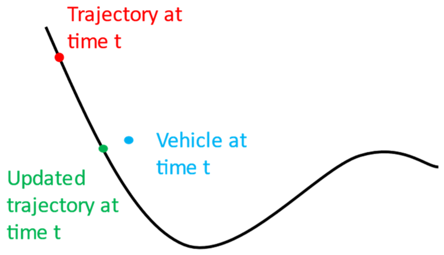
4.2.4. Path-Following Logic

The trajectory provided by guidance consists of a vector of variables to be tracked (i.e., position, velocity, and attitude) and the corresponding time. Referring to Figure 9, a common approach for trajectory tracking consists in targeting the reference variable at a given time instant (red point), no matter the current state of the vehicle (blue point). This strategy may not be optimal in presence of tracking errors of the GNC. An improvement to this approach is given by the path-following: here, the closest point to the vehicle on the trajectory is selected as the current setpoint and tracked (green point). Once this point is defined, and the corresponding control errors are computed with (45) and (46), the control of components ${\mathit{r}}_e\left(2\right), {\mathit{r}}_e\left(3\right)$ ensures reduction of the drift with respect to the desired path, while the control of the velocity ensures following the desired path (see [39] for the formal details and proofs of the method).

The main difficulty from an algorithmic standpoint is to estimate the closest point on the trajectory; it is also worth noting that the guidance only generates a discrete number of points corresponding to the nodes. The shape of the function between the nodes depends on the collocation method used; the use of the exact shape for the definition of the closest point can be very inefficient to implement onboard.

A simple way of approximating the trajectory between two nodes is to use a linear interpolation. On one hand, this approximation also introduces errors from a conceptual point of view, since a linear interpolation is only valid in the case of impulsive accelerations. On the other hand, its computational complexity is low.

A valid alternative, which improves the accuracy without excessively worsening the computational complexity, is given by the parabolic approximation. A common approach, indeed, is to consider the analytical solution of the linear kinematics when a zero-order hold on the control variables is used. In this case, the total forces acting on the vehicle are constant. This yields a constant acceleration ${\mathit{a}}_k$ in the trajectory time interval $t\in [t_k, t_{k+1}]$; so, the following relationships hold:

$${\mathit{v}}_g\left(t\right)={\mathit{v}}_k+{\mathit{a}}_k\left(t-t_k\right), t\in \left[t_k, t_{k+1}\right],$$

(51)

$${\mathit{r}}_g\left(t\right)={\mathit{r}}_k+{\mathit{v}}_k\left(t-t_k\right)+{\displaystyle \frac{1}{2}}{\mathit{a}}_k{\left(t-t_k\right)}^2.$$

(52)

As such, the trajectory is piecewise parabolic. The heuristic search of the closest point is then split into two parts:

Find the node at minimum distance from the actual position and define the interval in which the minimum is located (see Figure 10). The search is performed by finding the minimum of the elements in an array; this is quite efficient, as the array size provided by the guidance is small. By denoting with $s_k$ the closest trajectory node, it can be assumed that the closest point is either in the interval $\left[s_{k-1}, s_k\right]$ or $\left[s_k, s_{k+1}\right]$. Indeed, this is not necessarily true, but it is likely to happen in a re-entry trajectory.

Find the closest point on the considered arcs. This problem can be stated as an optimization problem in the following way: The trajectory $\gamma$ can be parametrized as a function of the Frenet–Serret parameter $s$ in the interval $\left[s_k, s_{k+1}\right]$ (equivalently in $\left[s_{k-1}, s_k\right]$), and it is possible to express the distance from the vehicle position ${\mathit{r}}_n$ to a generic point on the arc as

$$d^2\left(s\right)=\sum _{i=\mathrm{1,2},3}{\left({\displaystyle \frac{1}{2}}{\mathit{a}}_k\left(i\right)s^2+{\mathit{v}}_k\left(i\right)s+{\mathit{r}}_k\left(i\right)-{\mathit{r}}_n\left(i\right)\right)}^2.$$

(53)

Its derivatives with respect to the Frenet–Serret parameter $s$ can be derived analytically as

$${d^2}^{\prime }=\sum _{i=\mathrm{1,2},3}2\left({\displaystyle \frac{1}{2}}{\mathit{a}}_k\left(i\right)s^2+{\mathit{v}}_k\left(i\right)s+{\mathit{r}}_k\left(i\right)-{\mathit{r}}_n\left(i\right)\right)\left({\mathit{a}}_k\left(i\right)s+{\mathit{v}}_k\left(i\right)\right),$$

(54)

$${d^2}^{″}=\sum _{i=\mathrm{1,2},3}2\left({\left({\mathit{a}}_k\left(i\right)s+{\mathit{v}}_k\left(i\right)\right)}^2+{\mathit{a}}_k\left(i\right)\left({\displaystyle \frac{1}{2}}{\mathit{a}}_k\left(i\right)s^2+{\mathit{v}}_k\left(i\right)s+{\mathit{r}}_k\left(i\right)-{\mathit{r}}_n\left(i\right)\right)\right).$$

(55)

This stated, the closed point can be retrieved as the solution of the following constrained NLP:

$$\underset{s\in [s_k, s_{k+1}]}{\mathrm{m}\mathrm{i}\mathrm{n}\mathrm{i}\mathrm{m}\mathrm{i}\mathrm{z}\mathrm{e}} d^2(s).$$

(56)

This can be either solved analytically by using the Ferri–Cardano–Tartaglia Formulas [40] on the first-order optimality conditions or numerically through a Newton–Rapson procedure, such that

$$s_{opt}^{(j+1)}=s_{opt}^{\left(j\right)}-{\displaystyle \frac{{d^2}^{\prime }}{{d^2}^{″}}}.$$

(57)

where the superscript $j$ identifies the iterative solution. The same subproblem is solved in the interval $\left[s_{k-1}, s_k\right]$ and the minimum of the two minima is set as the closest point.

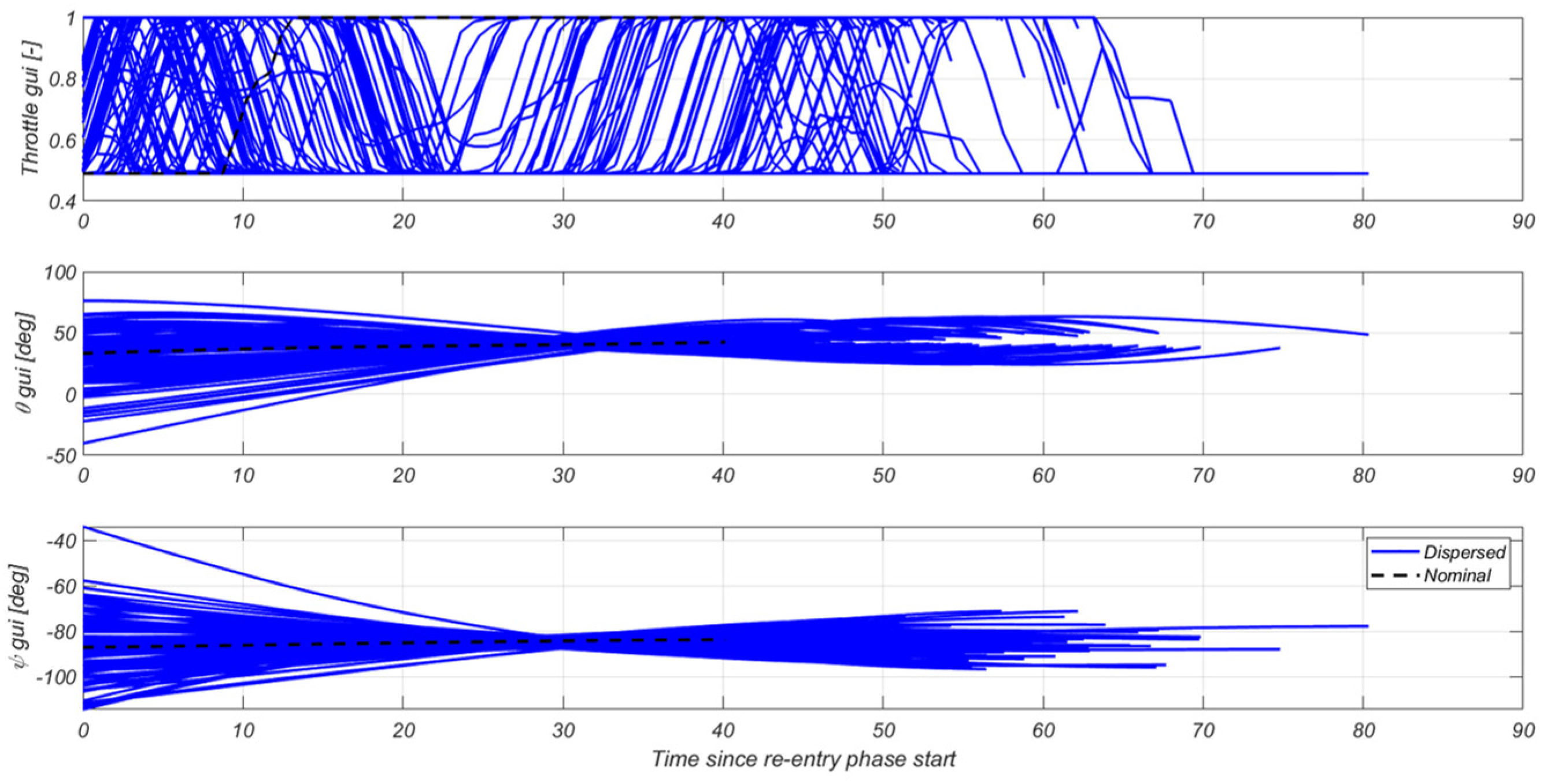
4.2.5. Re-Entry G&C Specific Results

This section reports the main results for the re-entry phase. As stated in Section 4.2.1, this is the phase of the mission in which the dispersions at MECO are recovered. The commands obtained are shown in Figure 11 for the nominal case (black) and considering dispersions (blue, see Section 5). As the initial conditions to trigger the re-entry burn vary a lot, the solutions obtained by the guidance can be quite different from one case to the other. The final time, indeed, adapts to the initial conditions as well. For what concerns the commanded attitude, the variability of the yaw angle can be related to the uncertainties on the heading angle at MECO; this translates into an increment (proportional to the ballistic flight time) of the cross-track error with respect to the nominal trajectory. A similar consideration applies to the pitch angle profiles that are related to the initial dispersions in groundspeed and flight path angle.

For what concerns the tracking errors, these are shown in Figure 12. During the first leg of the phase, the controller can very accurately track the desired reference path (i.e., ${\mathit{r}}_e\left(2\right), {\mathit{r}}_e\left(3\right)$), as well as the target velocity (i.e., ${\mathit{v}}_e\left(1\right))$. For some cases, at the end of the phase, the position error increases; for those runs, the vehicle needs to fly with high aerodynamic angles to compensate for the uncertainties on the MECO conditions. In such conditions, the aerodynamic forces are not negligible, and this violates the assumptions used for the guidance design. However, the induced errors are small if compared to the flight conditions and they have minor impact on the recovery strategy. The tracking errors are compensated in the next phases, namely, the aerodynamic and landing phases. The guidance will generate a new reference trajectory at the beginning of the next phase based on the current flight conditions, even if these conditions are diverged from the reference waypoint. Other strategies are still under investigation, for instance, a re-optimization in the same phase, as seen in [5].

4.3. Aerodynamic Phase

The objective of the G&C during the aerodynamic descent is to guide the first stage towards the initial conditions of the landing powered phase by means of the aerodynamic forces.

4.3.1. Aerodynamic Descent Guidance Design

Similarly to the re-entry burn phase, the guidance solves an optimal control problem. However, since the thrust is not available in this phase, the vehicle is controlled through the aerodynamic forces. These are generated thanks to the relative attitude of the vehicle with respect to the airflow. For this reason, the problem is formulated with a 5DoF model, using the attitude rates as control inputs. The dynamics is developed with respect to the ENU reference frame centered at the landing point. Thus, the problem formulation is the following:

$$\begin{array}{cc}\underset{\mathit{u},t_f}{\mathrm{m}\mathrm{i}\mathrm{n}\mathrm{i}\mathrm{m}\mathrm{i}\mathrm{z}\mathrm{e}}& J_{rnt}=w_u{{\displaystyle \int }}_0^{t_f}\left(u_{\psi }^2+u_{\theta }^2\right)dt\\ & \\ \mathrm{s}\mathrm{u}\mathrm{b}\mathrm{j}\mathrm{e}\mathrm{c}\mathrm{t} \mathrm{t}\mathrm{o}:& \dot{\mathit{x}}\left(t\right)={\mathit{f}}_{\mathit{a}\mathit{e}\mathit{r}\mathit{o}}(\mathit{x}\left(t\right),\mathit{u}\left(t\right))\\ & {\mathit{r}}_0={\overline{\mathit{r}}}_0, {\mathit{v}}_0={\overline{\mathit{v}}}_0, {\psi }_0={\overline{\psi }}_0, {\theta }_0={\overline{\theta }}_0 \\ & {\mathit{r}}_f={\overline{r}}_f, {\mathit{v}}_f={\overline{\mathit{v}}}_f\\ & \left|u_{\psi }\right|\le u_{ \psi ,max}, \left|u_{\theta }\right|\le u_{ \theta ,max}\\ & \left|{\dot{u}}_{\psi }\right|\le {\dot{u}}_{ \psi ,max}, \left|{\dot{u}}_{\theta }\right|\le {\dot{u}}_{ \theta ,max}\end{array}$$

(Problem 3)

where the state $\mathit{x}={\left[{\mathit{r}}^T,{\mathit{v}}^T,\psi ,\theta \right]}^T\in {\mathbb{R}}^8$ includes the position, the velocity, and the attitude angles, respectively. The control vector is defined as $\mathit{u}={\left[u_{\psi }, u_{\theta }\right]}^T\in {\mathbb{R}}^2$ and it includes commanded yaw rate and pitch rate. The problem accounts for the boundary conditions and the bounds on both inputs and control variables. ${\mathit{f}}_{\mathit{a}\mathit{e}\mathit{r}\mathit{o}}\in {\mathbb{R}}^8$ defines the dynamics constraints, as stated in (58):

$${\mathit{f}}_{aero}\left(\mathit{x},\mathit{u}\right)=\left[\begin{array}{c}\mathit{v}\\ {\mathit{a}}_{aero}^{ENU}+\mathit{g}+{\mathit{a}}_{\mathit{r}\mathit{o}\mathit{t}}\\ u_{\psi }\\ u_{\theta }\end{array}\right].$$

(58)

The aerodynamic accelerations are expressed in aerodynamic frame (AA) as

$${\mathit{a}}_{aero}^{AA}=-{\displaystyle \frac{1}{2m}}\rho S{\left|\left|\mathit{v}\right|\right|}^2\left[\begin{array}{c}{C}_D\left(\alpha ,M\right)\\ 0\\ C_L\left(\alpha ,M\right)\end{array}\right].$$

(59)

Since, the equations of motion are expressed in ENU reference frame, it is necessary to transform (59) in this way:

$${\mathit{a}}_{aero}^{ENU}=R_{BODY}^{ENU}\left(\theta ,\psi \right)R_{AA}^{BODY}\left(\alpha ,\beta \right){\mathit{a}}_{aero}^{AA},$$

(60)

where $\alpha ,\beta$ are the angle of attack and the sideslip angle, respectively. Of course, the aerodynamic contributions are a nonlinear combination of states and controls that must be convexified. In this phase, the problem assumes $C_Q=0$, since a zero-sideslip roll maneuver is considered (Section 4.3.2).

The cost function only includes the terms relative to the control effort to obtain smooth maneuvers that the control can track more efficiently.

As performed for the re-entry phase (Section 4.2), (Problem 3) considers a ZOH parametrization of the control variables and the dynamic constraints are mapped into their discrete time version by using a forward Euler integration scheme; this allows for obtaining ${\mathit{F}}_{\mathit{a}\mathit{e}\mathit{r}\mathit{o}}\left(\mathit{x},\mathit{u},\Delta t\right)$ in a similar form of (22). Then, (Problem 3) is convexified by linearizing the dynamics constraints (${\displaystyle \frac{\mathbf{\partial }{\mathit{F}}_{\mathit{a}\mathit{e}\mathit{r}\mathit{o}}}{\mathbf{\partial }(.)}}$) and the cost function (${\displaystyle \frac{\mathbf{\partial }{J}_{aero}}{\mathbf{\partial }(.)}}$). Also in this case, soft trust regions are applied to the control variables and the final time to avoid artificial unboundedness and limit the variation in optimization variables between the iterations of the SCP. Concerning virtual controls, a trade-off analysis was performed to define whether they are necessary or not, and the conclusion shows the virtual controls can only be applied to the states of the last node, more precisely the velocity components. In other words, a soft relaxation of the final conditions constraint is implemented. Thus, this becomes

$$\begin{array}{c}{A}_f\mathit{x}+S_P{\mathit{s}}_{\mathit{p}}+S_n{\mathit{s}}_{\mathit{n}}={\mathit{b}}_{\mathit{f}}\end{array},$$

(61)

where ${\mathit{s}}_{\mathit{p}}$ and ${\mathit{s}}_{\mathit{n}}$ are additional slack variables that are penalized in the cost function with an associated weight $w_h$; $S_p$ and $S_n$ are selector matrices that in this case only apply the relaxation to the velocity components. This allows for a reduced number of optimization variables, enhancing computational efficiency.

Considering the same procedure reported for the re-entry phase and the considerations addressed above, the convexified formulation of (Problem 3) reads as follows:

$$\begin{array}{cc}\underset{{\mathit{x}}_{opt,aug}}{\mathrm{m}\mathrm{i}\mathrm{n}\mathrm{i}\mathrm{m}\mathrm{i}\mathrm{z}\mathrm{e}}& J_{aero,CVX}={\displaystyle \frac{w_u{\widehat{t}}_f}{N-1}} {\displaystyle \sum _k}{S_u,}_k+{\displaystyle \frac{1}{N-1}}\left(w_u{\displaystyle \sum _k}{\widehat{S}}_{u,k}\right)t_f+w_h{\mathbf{1}}^{\mathit{T}}{\mathit{s}}_{\mathit{p}}-w_h{\mathbf{1}}^{\mathit{T}}{\mathit{s}}_{\mathit{n}}+w_{\xi }{S}_{\xi }+w_{\xi ,t_f}{\xi }_{t_f}\\ & \\ \mathrm{s}\mathrm{u}\mathrm{b}\mathrm{j}\mathrm{e}\mathrm{c}\mathrm{t} \mathrm{t}\mathrm{o}:& A_{dyn,k}{\mathit{x}}_{\mathit{o}\mathit{p}\mathit{t},\mathit{k}}={\mathit{b}}_{dyn,k} \mathrm{f}\mathrm{o}\mathrm{r} k=1,\dots ,N-1\\ & A_0\mathit{x}={\mathit{b}}_{\mathbf{0}} \\ & A_f\mathit{x}+S_P{\mathit{s}}_{\mathit{p}}+S_n{\mathit{s}}_{\mathit{n}}={\mathit{b}}_{\mathit{f}}\\ & \left|u_{\psi ,k}\right|\le u_{ \psi ,max}, \left|u_{\theta ,k}\right|\le u_{ \theta ,max}, \left|u_{T,k}\right|\le u_{ T,max}\\ & \left|{(u}_{\psi ,k+1}-u_{\psi ,k})\right|\le {\dot{u}}_{ \psi ,max}\Delta t, \left|{(u}_{\theta ,k+1}-u_{\theta ,k})\right|\le {\dot{u}}_{ \theta ,max}\Delta t\\ & {\mathit{u}}_{\mathit{k}}-{\widehat{\mathit{u}}}_{\mathit{k}}={\mathit{\xi }}_{\mathit{k}} \mathrm{f}\mathrm{o}\mathrm{r} k=1,\dots ,N\\ & {\left|\left|{\mathit{\xi }}_{\mathit{k}}\right|\right|}_{\mathbf{2}}\le {\mathbf{\Delta }}_{\mathit{k}}\\ & {\displaystyle \sum _{\mathit{k}}}{\mathbf{\Delta }}_k=S_{\xi }\\ & {\left|\left|t_f-{\widehat{t}}_f\right|\right|}_{\mathbf{2}}={\xi }_{{\mathit{t}}_{\mathit{f}}}\\ & u_{\psi ,k}^2+u_{\theta ,k}^2\le S_{u,k}.\end{array}$$

(Problem 4)

Stacking the variables in a 1D vector, (Problem 4) can be rewritten as an SOCP by means of augmented matrices for equality and inequality constraints. The complete optimization vector is

$${\mathit{x}}_{opt,aug}:={\left[\begin{array}{cccccccccc}{\mathit{x}}_{1\times 8\ast N}& {\mathit{u}}_{1\times 2\ast N}& t_f& {\mathit{s}}_{\mathit{p},1\times \mathbf{3} }& {\mathit{s}}_{\mathit{n},,1\times \mathbf{3}}& {\mathit{\xi }}_{1\times 3\ast N}& {\mathbf{\Delta }}_{1\times N}& S_{\xi }& S_{\xi ,tf}& S_{u,1\times N}\end{array}\right]}^T.$$

(62)

4.3.2. Roll Command for Zero-Sideslip

For the aerodynamic phase, a symmetric flight condition is considered, such that the aerodynamic coefficients only depend on the angle of attack and Mach number. This assumption leverages on the following considerations:

• The vehicle is symmetrical, so its aerodynamic properties are optimal. To make this assumption, we neglect the impact of the fins on the AEDB symmetry characteristics and winds (which we assume negligible compared to the airspeed for guidance purposes for this phase of flight).
• The roll angle is such that the sideslip angle is zero. The value of this angle can be found via the definition of the sideslip angle as

$$\beta =\mathrm{asin}\left({\displaystyle \frac{v}{V}}\right),$$

(63)

meaning that $v=0\to \beta =0.$ The value of $v$ can be related to the states of the optimization problem via the rotation matrix as

$$\begin{array}{c}v=\left(\mathrm{s}\mathrm{i}\mathrm{n}\varphi \mathrm{s}\mathrm{i}\mathrm{n}\theta \mathrm{c}\mathrm{o}\mathrm{s}\psi -\mathrm{c}\mathrm{o}\mathrm{s}\varphi \mathrm{s}\mathrm{i}\mathrm{n}\psi \right)\mathit{v}\left(1\right)+\left(\mathrm{s}\mathrm{i}\mathrm{n}\varphi \mathrm{s}\mathrm{i}\mathrm{n}\theta \mathrm{s}\mathrm{i}\mathrm{n}\psi +\mathrm{c}\mathrm{o}\mathrm{s}\varphi \mathrm{c}\mathrm{o}\mathrm{s}\psi \right)\mathit{v}\left(2\right)\\ \hspace{1em}\hspace{1em}\hspace{1em}\hspace{1em}\hspace{1em}\hspace{1em}+\mathrm{c}\mathrm{o}\mathrm{s}\theta \mathrm{s}\mathrm{i}\mathrm{n}\varphi \mathit{v}\left(3\right),\end{array}$$

(64)

such that imposing $v=0$ yields

$$\begin{array}{c}\mathrm{s}\mathrm{i}\mathrm{n}\varphi \left(\mathrm{s}\mathrm{i}\mathrm{n}\theta \mathrm{c}\mathrm{o}\mathrm{s}\psi \mathit{v}\left(1\right)+\mathrm{s}\mathrm{i}\mathrm{n}\theta \mathrm{s}\mathrm{i}\mathrm{n}\psi \mathit{v}\left(2\right)+\mathrm{c}\mathrm{o}\mathrm{s}\theta \mathit{v}\left(3\right)\right)\\ \hspace{1em}\hspace{1em}\hspace{1em}\hspace{1em}\hspace{1em}\hspace{1em}+\mathrm{c}\mathrm{o}\mathrm{s}\varphi \left(-\mathrm{s}\mathrm{i}\mathrm{n}\psi \mathit{v}\left(1\right)+\mathrm{c}\mathrm{o}\mathrm{s}\psi \mathit{v}\left(2\right)\right)=0.\end{array}$$

(65)

This relationship can be rearranged to find the value of the roll angle for the zero-sideslip condition

$$\varphi =\mathrm{atan}\left({\displaystyle \frac{\mathrm{s}\mathrm{i}\mathrm{n}\psi \mathit{v}\left(1\right)-\mathrm{c}\mathrm{o}\mathrm{s}\psi \mathit{v}\left(2\right)}{\mathrm{s}\mathrm{i}\mathrm{n}\theta \mathrm{c}\mathrm{o}\mathrm{s}\psi \mathit{v}\left(1\right)+\mathrm{s}\mathrm{i}\mathrm{n}\psi \mathrm{s}\mathrm{i}\mathrm{n}\theta \mathit{v}\left(2\right)+\mathrm{c}\mathrm{o}\mathrm{s}\theta \mathit{v}\left(3\right)}}\right).$$

(66)

4.3.3. Aerodynamic Descent Control Design

The architecture for the aerodynamic controller features a cascaded scheme in which an inner attitude controller tracks the reference attitude prescribed by the guidance function. An outer control loop adds modifications to the reference attitude to limit the position dispersions with respect to the reference trajectory. As the phase is unpowered, it is not possible to track the reference trajectory with high accuracy. In particular, uncertainties on the aerodynamic coefficients have a relevant impact on the vehicle downrange correction capability. For this reason, attitude corrections from the outer loop are limited within a threshold to avoid unrealistic (i.e., outside the linearity assumptions) and ineffective commands (higher commands imply an increment of the aerodynamic loads).

Similarly to the structure presented in Section 4.2.3, the pitch attitude controller features the following control logic:

$${\delta }_{f,\theta }=K_{\theta }{\theta }_e+K_q{q}_e+K_w{w}_e,$$

(67)

where the term $w_e$ denotes the error on the z component of the body velocity (equivalent to AoA feedback). A similar law is used for the yaw channel. As we mentioned above, the reference tracked by the controller is a combination of the computed guidance attitude and position error compensation outer loop. The latter contribution is given by the following PD-like logic:

$$\begin{array}{c}{\varphi }_{trk}=\\ {\theta }_{trk}=\\ {\psi }_{trk}=\end{array} \begin{array}{c}0,\\ F_1\left(K_Z{r}_e\left(3\right)+{F_{2}K}_{\dot{Z}}{v}_e\left(3\right)\right),\\ F_1\left(K_Y{r}_e\left(2\right)+{F_{2}K}_{\dot{Y}}{v}_e\left(2\right)\right),\end{array}$$

(68)

where $F_1, F_2$ denote lowpass filters used to ensure inner–outer loop timescale separation. The reference attitude to be tracked by the inner loop $R_r$ can be then computed starting from the profile of the guidance $R_g$ and the outer loop corrections $\Delta R_o$(i.e., the rotation matrix corresponding to the outer loop attitude corrections) as follows:

$$R_r=\Delta R_o{R}_g.$$

(69)

The new reference angular velocity ${\mathit{\omega }}_r$ can be computed starting from the corrections and the guidance velocity ${\mathit{\omega }}_g$ by combination of the angular velocities [35] (pp. 67–122) as

$${\mathit{\omega }}_r=\Delta R_o{\mathit{\omega }}_g+S\left({\theta }_{trk}\right)\left[\begin{array}{c}0\\ {\dot{\theta }}_{trk}\\ {\dot{\psi }}_{trk}\end{array}\right],$$

(70)

with

$$S\left({\theta }_{trk}\right)=\left[\begin{array}{ccc}1& 0& -\mathrm{s}\mathrm{i}\mathrm{n}{\theta }_{trk}\\ 0& 1& 0\\ 0& 0& \mathrm{c}\mathrm{o}\mathrm{s}{\theta }_{trk}\end{array}\right].$$

(71)

A feedforward command is also considered in the control logic. This command is defined as the nominal fin deflection to achieve zero aerodynamic torque in nominal condition. This deflection is defined as a function of the aerodynamic angles and Mach and it is superimposed to the feedback command (67). Similarly to the re-entry controller, the path following the logic explained in Section 4.2.4 is used to extract the reference points to be tracked. The functional architecture for the aerodynamic controller can be found in Figure 13.

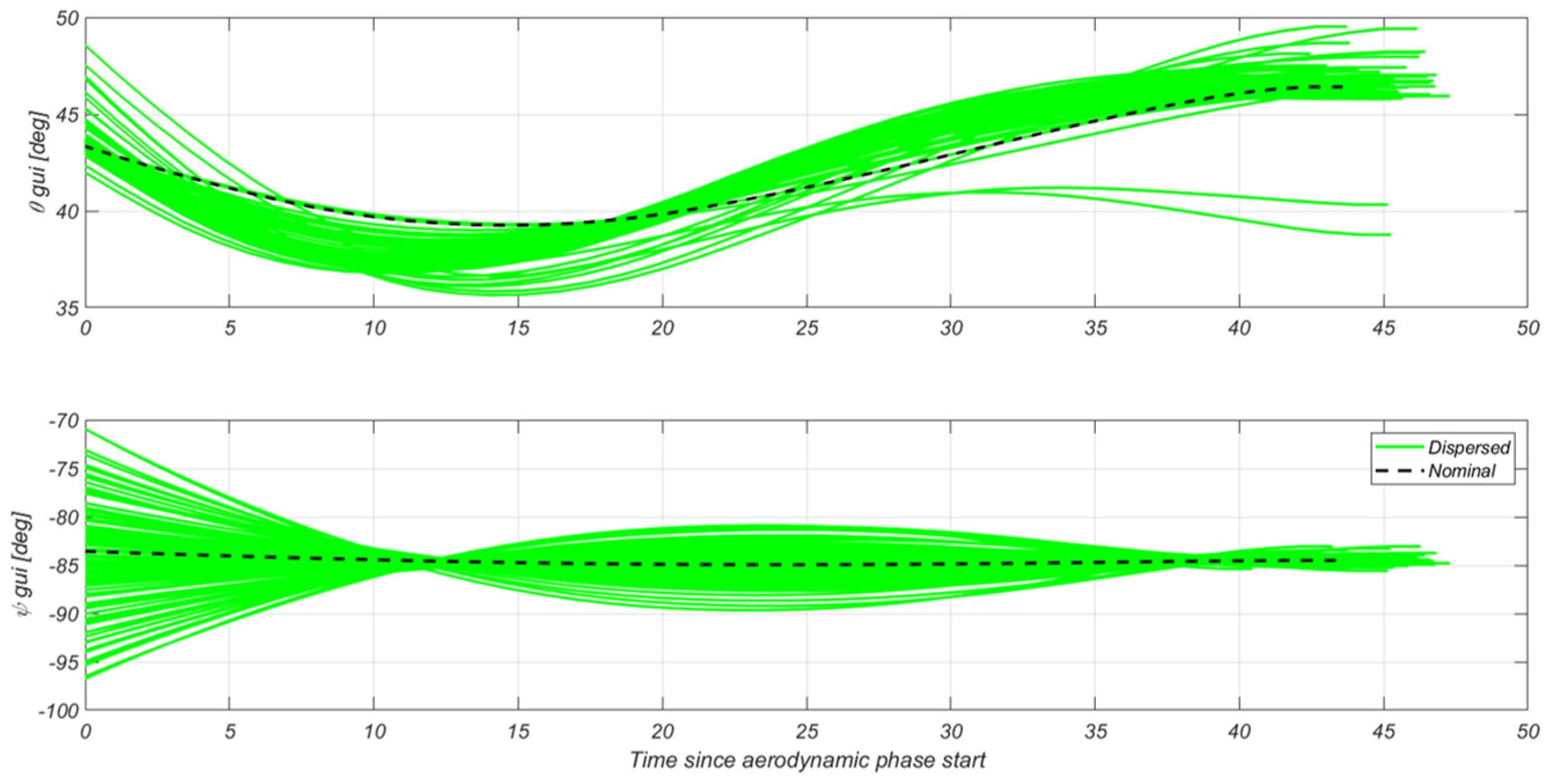
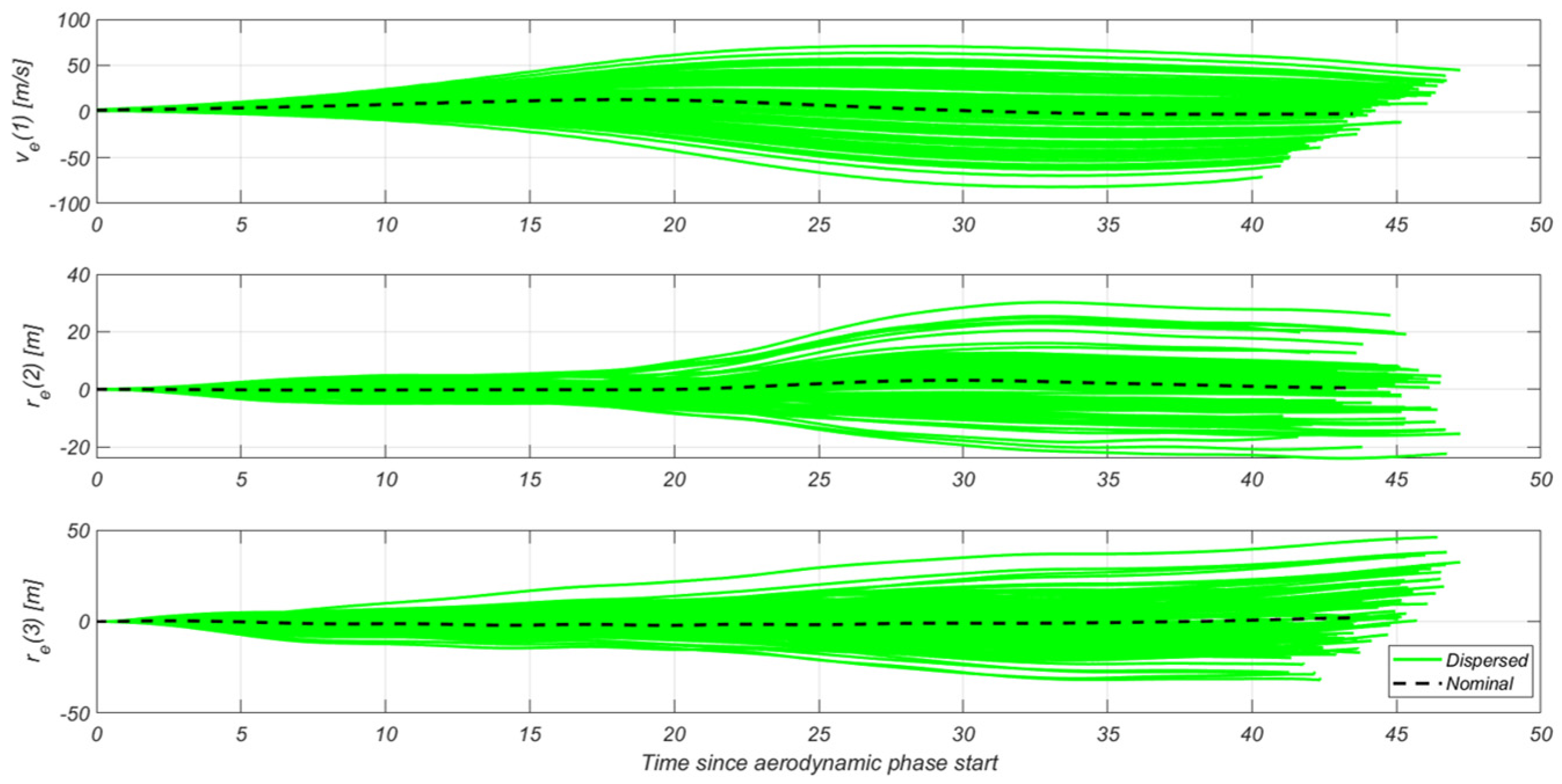
4.3.4. Aerodynamic G&C-Specific Results

This section reports the main results for the aerodynamic phase. The guidance commands are shown in Figure 14. In this case, variability in the angles is needed to generate the necessary aerodynamic forces to target the desired waypoint.

For what concerns the tracking errors, these are shown in Figure 15. As this phase is unpowered, only a subset of the states of the vehicle can be controlled, and in the presence of uncertainties in the aerodynamic coefficients, the vehicle drifts from the desired reference path. The control strategy described in Section 4.3.3 aims at reducing the lateral drift, while no control on the vehicle velocity is exerted. The velocity errors are compensated during the landing phase. By direct inspection of Figure 15, it can be seen that the control is capable of containing the drift with respect to the reference path; however, as the aerodynamic forces are only used to correct the position, the dispersion in velocity increases, and the higher the uncertainty on the aerodynamic coefficients, the larger this dispersion interval at the end of the phase. When the guidance has exact knowledge of the aerodynamic properties, the vehicle can accurately follow the desired reference path (black line).

4.4. Landing Burn Phase

The objective of the G&C during the landing phase is to guide the first stage towards the target landing site and perform a precise pinpoint landing. This phase is of fundamental importance since the dispersions in position and velocity accumulated during the aerodynamic descent must be compensated. In this phase, the environment is considerably challenging especially for the nonnegligible effect of winds.

4.4.1. Powered Landing Guidance Design

As in the re-entry phase, the guidance solves the 5DoF free final time fuel-optimal powered pinpoint landing problem to obtain onboard a reference trajectory that is provided to the control. The problem is formulated in an East–North–Up (ENU) reference frame centered at the landing point. In this phase, the optimization problem account for aerodynamics forces and AoA constraints. Moreover, due to the relative low velocity, a wind speed profile is explicitly considered in the problem formulation. The problem is the following:

$$\begin{array}{cc}\underset{\mathit{u},t_f}{\mathrm{m}\mathrm{i}\mathrm{n}\mathrm{i}\mathrm{m}\mathrm{i}\mathrm{z}\mathrm{e}}& J_{lnd}=w_T{{\displaystyle \int }}_0^{t_f}Tdt+w_u{{\displaystyle \int }}_0^{t_f}\left(u_{\psi }^2+u_{\theta }^2\right)dt\\ & \\ \mathrm{s}\mathrm{u}\mathrm{b}\mathrm{j}\mathrm{e}\mathrm{c}\mathrm{t} \mathrm{t}\mathrm{o}:& \dot{\mathit{x}}\left(t\right)={\mathit{f}}_{\mathit{l}\mathit{n}\mathit{d}}(\mathit{x}\left(t\right),\mathit{u}\left(t\right))\\ & {\mathit{r}}_0={\overline{\mathit{r}}}_0, {\mathit{v}}_0={\overline{\mathit{v}}}_0,m_0={\overline{m}}_0, {\psi }_0={\overline{\psi }}_0, {\theta }_0={\overline{\theta }}_0 \\ & {\mathit{r}}_f=\overline{{\mathit{r}}_f}, {\mathit{v}}_f={\overline{\mathit{v}}}_f, {\psi }_f={\overline{\psi }}_f, {\theta }_f={\overline{\theta }}_f\\ & T_{min }\le T\le T_{max} \\ & \left|u_{\psi }\right|\le u_{ \psi ,max}, \left|u_{\theta }\right|\le u_{ \theta ,max}, \left|u_T\right|\le u_{ T,max}\\ & \left|{\dot{u}}_{\psi }\right|\le {\dot{u}}_{ \psi ,max}, \left|{\dot{u}}_{\theta }\right|\le {\dot{u}}_{ \theta ,max}\\ & \left[\begin{array}{ccc}\cos \psi \cos \theta & \sin \psi \cos \theta & \sin \theta \end{array}\right]{\displaystyle \frac{\mathit{v}}{{\left|\left|\mathit{v}\right|\right|}_2}}\le \cos {\alpha }_{max}\end{array}$$

(Problem 5)

where the state $\mathit{x}={\left[{\mathit{r}}^T,{\mathit{v}}^T,m,\psi ,\theta ,T\right]}^T\in {\mathbb{R}}^{10}$ embeds the position, the velocity with respect to the ground, the mass, the yaw and pitch angles, and the thrust magnitude, respectively. The control vector $\mathit{u}={\left[u_{\psi }, u_{\theta }, u_T\right]}^T\in {\mathbb{R}}^3$ defines the commanded yaw rate, pitch rate, and thrust rate. In the problem, the boundary conditions and the bounds on both inputs and control variables are imposed. The dynamics constraint ${\mathit{f}}_{\mathit{l}\mathit{n}\mathit{d}}\in {\mathbb{R}}^{10}$ represents the flat-Earth 5DoF powered-rocket dynamics

$${\mathit{f}}_{\mathit{l}\mathit{n}\mathit{d}}\left(\mathit{x},\mathit{u}\right)=\left[\begin{array}{c}\mathit{v}\\ {\displaystyle \frac{T}{m}}{\mathit{i}}_T\left(\psi ,\theta \right)+{\mathit{a}}_{aero}^{ENU}+\mathit{g}+{\mathit{a}}_{\mathit{r}\mathit{o}\mathit{t}}\\ -{\displaystyle \frac{1}{I_{sp}{g}_0}}T\\ u_{\psi }\\ u_{\theta }\\ u_T\end{array}\right],$$

(72)

with ${\mathit{i}}_T={\left[\cos \psi \cos \theta , \sin \psi \cos \theta ,-\sin \theta \right]}^T$, ${\mathit{a}}_{\mathit{r}\mathit{o}\mathit{t}}$ is the acceleration due to the Earth rotation, and ${\mathit{a}}_{\mathit{a}\mathit{e}\mathit{r}\mathit{o}}$ are the aerodynamics acceleration in ENU reference frame. In this context, the aerodynamic accelerations expressed in the aerodynamic frame (AA) are stated as follows:

$${\mathit{a}}_{aero}^{AA}=-{\displaystyle \frac{1}{2m}}\rho S{\left|\left|{\mathit{v}}_{\mathit{a}}\right|\right|}^2\left[\begin{array}{c}{C}_D\left(\alpha ,\beta ,M\right)\\ C_Q\left(\beta ,M\right)\\ C_L\left(\alpha ,M\right)\end{array}\right].$$

(73)

Concerning the aerodynamic effects, the following considerations are made:

• The aerodynamics coefficients are approximated with splines in order to have smoother profiles. In this phase, the side force is also taken into account, and due to the symmetry of the vehicle, $C_Q$ is modelled as the $C_L$.
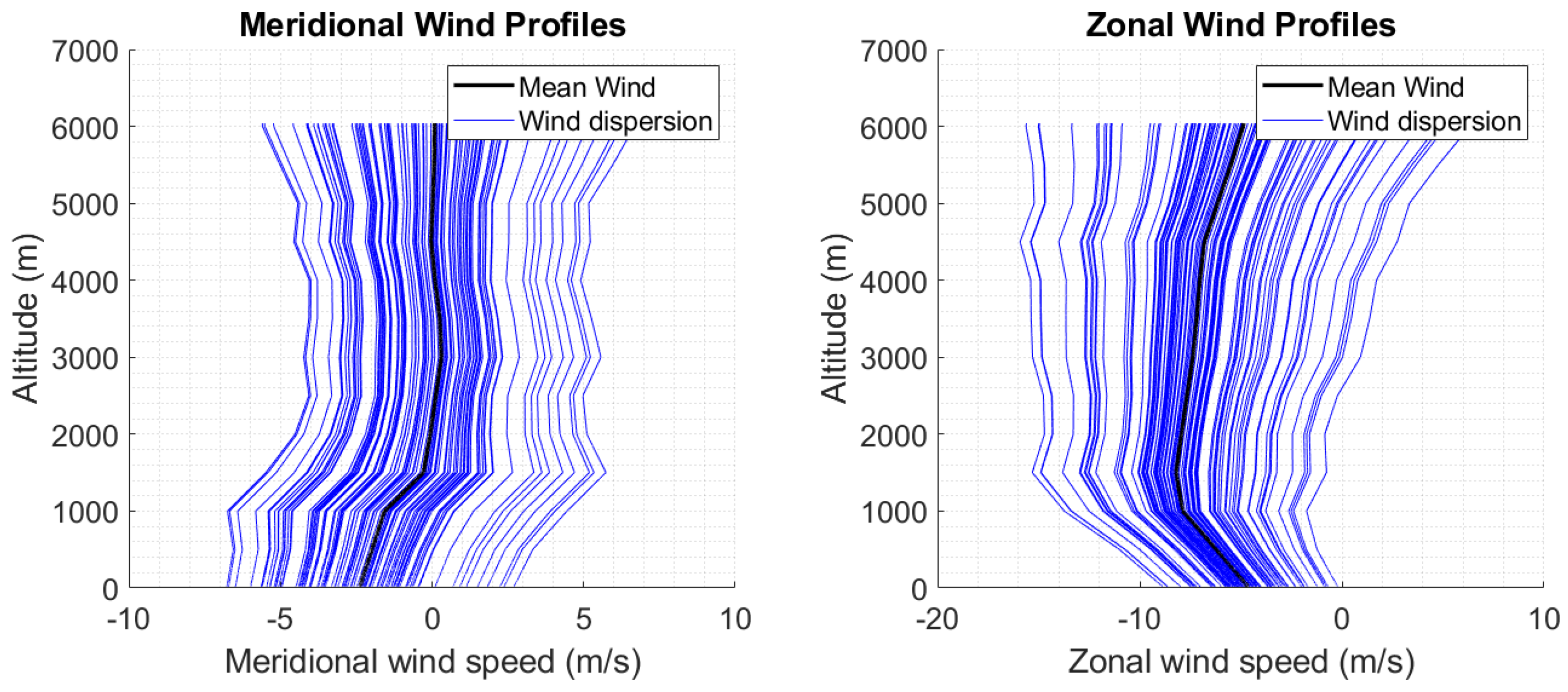
• Since a wind profile is considered, the velocity of the vehicle with respect to the ground and the one respect to the air do not coincide, so

$${\mathit{v}}_{\mathit{a}}=\mathit{v}-{\mathit{v}}_{\mathit{w}}^{ENU}.$$

(74)

The aerodynamic angles must be defined accordingly.

• The wind speed profile ${\mathit{v}}_{\mathit{w}}$ is assumed to be a function of the altitude only. The guidance knows the mean wind value at the mission epoch (Figure 16). During the simulations, uncertainties on the wind are considered.
• The formulation of the dynamics equation by considering the relative velocity introduces additional terms in the computation of the Jacobians during the convexification step, since

$${\displaystyle \frac{\mathbf{\partial }{\mathit{v}}_{\mathit{a}}}{\mathbf{\partial }{r}_z}}=-{\displaystyle \frac{\mathbf{\partial }{\mathit{v}}_{\mathit{w}}\left(r_z\right)}{\mathbf{\partial }{r}_z}}.$$

(75)

Figure 16. Mean meridional and zonal local wind model for Kourou, French Guyana [41].

Figure 16. Mean meridional and zonal local wind model for Kourou, French Guyana [41].

The cost function used for this phase is equal to the objective of the re-entry, where the goal is the minimization of the fuel mass needed for the maneuver and the minimization of the attitude control effort. In this case, (Problem 5) accounts for a limitation of the total AoA with respect to the ground, defined as a nonlinear constraint; this is to meet trim and stability requirements defined during the mission analysis. Moreover, since the uncertainties on the winds play a significant role, the smaller the AoA, the smaller the wind-induced perturbations. As calculated for the re-entry and the aerodynamic phases, (Problem 5) is discretized using the forward Euler scheme to obtain ${\mathit{F}}_{\mathit{l}\mathit{n}\mathit{d}}\left(\mathit{x},\mathit{u},\Delta t\right)$. Consequently, the nonlinear dynamics constraints (${\displaystyle \frac{\mathbf{\partial }{\mathit{F}}_{\mathit{l}\mathit{n}\mathit{d}}}{\mathbf{\partial }(.)}}$), the relaxed AoA constraint (${\displaystyle \frac{\mathbf{\partial }{\mathrm{g}}_{aoa}}{\mathbf{\partial }(.)}}$), and the cost function (${\displaystyle \frac{\mathbf{\partial }{J}_{lnd}}{\mathbf{\partial }(.)}}$) are convexified through a First-Order Taylor expansion.

A relaxation of the AoA constraint is performed to improve the convergence and reduce the computational effort. Consider $g_{aoa}\left({\mathit{x}}_{\mathit{k}},{\mathit{u}}_{\mathit{k}}\right)\le 0$ as the nonlinear equation that describes the AoA constraint at each node; the relaxation is calculated in the following way:

$$g_{aoa}\left({\widehat{\mathit{x}}}_k,{\widehat{\mathit{u}}}_k\right)+{\displaystyle \frac{\partial g_{aoa}}{\partial \mathit{x}}}\left({\mathit{x}}_k-{\widehat{\mathit{x}}}_k\right)+{\displaystyle \frac{\partial g_{aoa}}{\partial \mathit{u}}}\left({\mathit{u}}_k-{\widehat{\mathit{u}}}_k\right) \le {\mathit{s}}_{\mathit{a}\mathit{o}\mathit{a}} ,\forall k\in \left[1, K\right],$$

(76)

where ${\mathit{s}}_{aoa}$ is a vector of slack variables $\in {\mathbb{R}}^K$, and K is the number of nodes. Furthermore, two constraints are added to limit the norm of this vector, by using an additional variable as follows:

$$-{\Delta }_{aoa}\le 0$$

(77)

$${\left|\left|{\mathit{s}}_{aoa}\right|\right|}_2\le {\Delta }_{aoa}.$$

(78)

Finally, ${\Delta }_{aoa}$ is minimized in the cost function.

Soft trust regions are applied to the control variables and the final time to avoid artificial unboundedness, and virtual controls on the vertical component of the velocity ($\mathit{v}\left(3\right)$) are applied (so the matrix $A_{\nu ,k}$ changes accordingly). Also in this case, only a minimum contribution of virtual controls is added to reduce the number of additional variables needed.

Following the same procedure reported for the re-entry and aerodynamic phases, the convexified formulation of (Problem 6) is

$$\begin{array}{cc}\underset{{\mathit{x}}_{opt,aug}}{\mathrm{m}\mathrm{i}\mathrm{n}\mathrm{i}\mathrm{m}\mathrm{i}\mathrm{z}\mathrm{e}}& J_{lnd,CVX}={\displaystyle \frac{w_T{\widehat{t}}_f}{N-1}} {\displaystyle \sum _k}{T}_k+{\displaystyle \frac{w_u{\widehat{t}}_f}{N-1}} {\displaystyle \sum _k}{S_u,}_k+{\displaystyle \frac{1}{N-1}}\left(w_T{\displaystyle \sum _k}{\widehat{T}}_k+w_u{\displaystyle \sum _k}{\widehat{S}}_{u,k}\right)t_f+\\ & +w_{\nu }{S}_{\nu }+w_{\xi }{S}_{\xi }+w_{\xi ,t_f}{\xi }_{t_f}+w_{aoa}{\Delta }_{aoa}\\ & \\ \mathrm{s}\mathrm{u}\mathrm{b}\mathrm{j}\mathrm{e}\mathrm{c}\mathrm{t} \mathrm{t}\mathrm{o}:& \left[A_{dyn,k} A_{\nu ,k}\right]\left[\begin{array}{c}{\mathit{x}}_{\mathit{o}\mathit{p}\mathit{t},\mathit{k}}\\ {\mathit{\nu }}_{\mathit{k}}\end{array}\right]={\mathit{b}}_{dyn,k} \mathrm{f}\mathrm{o}\mathrm{r} k=1,\dots ,N-1\\ & A_0\mathit{x}={\mathit{b}}_{\mathbf{0}} \\ & A_f\mathit{x}={\mathit{b}}_f\\ & { T}_{min }\le T_k\le T_{max} \mathrm{f}\mathrm{o}\mathrm{r} k=1,\dots ,N\\ & \left|u_{\psi ,k}\right|\le u_{ \psi ,max}, \left|u_{\theta ,k}\right|\le u_{ \theta ,max}, \left|u_{T,k}\right|\le u_{ T,max}\\ & \left|{(u}_{\psi ,k+1}-u_{\psi ,k})\right|\le {\dot{u}}_{ \psi ,max}\Delta t, \left|{(u}_{\theta ,k+1}-u_{\theta ,k})\right|\le {\dot{u}}_{ \theta ,max}\Delta t\\ & g_{aoa}\left({\widehat{\mathit{x}}}_k, {\widehat{\mathit{u}}}_{\mathit{k}}\right)+{\displaystyle \frac{\mathbf{\partial }{g}_{aoa}}{\mathbf{\partial }\mathit{x}}}\left({\mathit{x}}_{\mathit{k}}-{\widehat{\mathit{x}}}_k\right)+{\displaystyle \frac{\mathbf{\partial }g}{\mathbf{\partial }\mathit{u}}}\left({\mathit{u}}_{\mathit{k}}-{\widehat{\mathit{u}}}_{\mathit{k}}\right)\\ & {\left|\left|{\mathit{s}}_{aoa}\right|\right|}_2\le {\Delta }_{aoa}\\ & -{\Delta }_{aoa}\le 0\\ & {\left|\left|{\mathit{\nu }}_{\mathit{k}}\right|\right|}_{\mathbf{2}}\le {\mathit{\eta }}_{\mathit{k}} \mathrm{f}\mathrm{o}\mathrm{r} k=1,\dots ,N-1\\ & {\left|\left|{\mathit{\eta }}_{\mathit{k}}\right|\right|}_{\mathbf{2}}\le S_{\nu }\\ & {\mathit{u}}_{\mathit{k}}-{\widehat{\mathit{u}}}_{\mathit{k}}={\mathit{\xi }}_{\mathit{k}} \mathrm{f}\mathrm{o}\mathrm{r} k=1,\dots ,N\\ & {\left|\left|{\mathit{\xi }}_{\mathit{k}}\right|\right|}_{\mathbf{2}}\le {\mathbf{\Delta }}_{\mathit{k}}\\ & {\displaystyle \sum _{\mathit{k}}}{\mathbf{\Delta }}_k=S_{\xi }\\ & {\left|\left|t_f-{\widehat{t}}_{\mathit{f}}\right|\right|}_{\mathbf{2}}={\xi }_{{\mathit{t}}_{\mathit{f}}}\\ & u_{\psi ,k}^2+u_{\theta ,k}^2\le S_{u,k}.\end{array}$$

(Problem 6)

(Problem 6) is then transformed into the SOCP formulation. In this case, the stacked 1D optimization vector is

$$\begin{gathered} {\mathit{x}}_{opt,aug}:= \\ {\left[\begin{array}{ccccccccccccc}{\mathit{x}}_{1\times 10\ast N}& {\mathit{u}}_{1\times 3\ast N}& t_f& {\mathit{\nu }}_{1\times 2\ast \left(N-1\right)}& {\mathit{\eta }}_{1\times \left(N-1\right)}& S_{\nu }& {\mathit{\xi }}_{1\times 3\ast N}& {\mathbf{\Delta }}_{1\times N}& S_{\xi }& S_{\xi ,tf}& S_{u,1\times N}& {\mathit{s}}_{\mathit{a}\mathit{o}\mathit{a},\mathbf{1}\times \mathit{N}}& {\Delta }_{aoa}\end{array}\right]}^T \end{gathered}$$

(79)

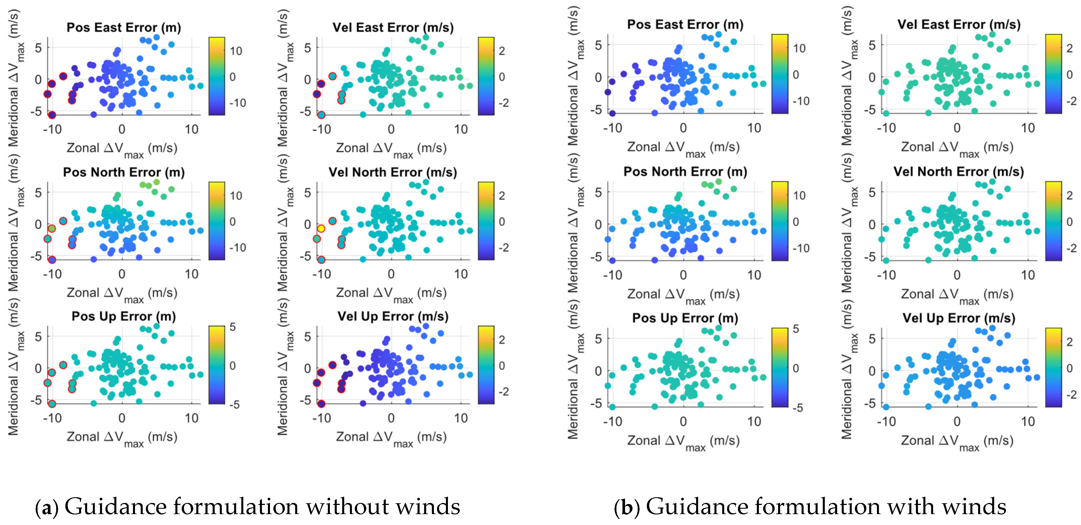
4.4.2. Benefits of the Wind Knowledge in the Landing Guidance

In this section, the benefits about considering the knowledge of the winds within the landing algorithm are discussed. The knowledge of the winds is introduced by loading the nominal wind table (Figure 16).

Figure 17 reports the results of two Monte-Carlo analyses of the landing phase where in one case (left), the guidance does not consider the presence of winds, while for the second case (right), it accounts for the nominal wind profile expected at the mission epoch. The results show that the inclusion of the winds allows for improving the landing accuracy, especially in the case of strong winds (bottom left dispersion region). For this analysis, uncertainties in initial conditions, MCI, aerodynamics, atmosphere, and winds are applied to the problem (see Section 4.4.4). Note that the simulations consider relatively high wind dispersions; on the contrary, in a real mission scenario, better estimation of the winds can be achieved before the launch.

Figure 17. Position and velocity errors at touchdown with respect to wind dispersion. The red dots highlight the trajectories that do not fulfil the landing requirements (Table 5).

Figure 17. Position and velocity errors at touchdown with respect to wind dispersion. The red dots highlight the trajectories that do not fulfil the landing requirements (Table 5).

Table 5. Landing requirements in ENU frame.

Landing Requirements	Value
East position	$-15 \mathrm{m}\le r_{East}\le 15 \mathrm{m}$
North position	$-15 \mathrm{m}\le r_{North}\le 15 \mathrm{m}$
East velocity	$-3 \mathrm{m}/\mathrm{s}\le v_{East}\le 3 \mathrm{m}/\mathrm{s}$
North velocity	$-3 \mathrm{m}/\mathrm{s}\le v_{East}\le 3 \mathrm{m}/\mathrm{s}$
Vertical velocity	$\left|\left|v_{Up}\right|\right|\le 3 \mathrm{m}/\mathrm{s}$
Pitch	$\theta \ge 85º$

Table 5. Landing requirements in ENU frame.

Landing Requirements	Value
East position	$-15 \mathrm{m}\le r_{East}\le 15 \mathrm{m}$
North position	$-15 \mathrm{m}\le r_{North}\le 15 \mathrm{m}$
East velocity	$-3 \mathrm{m}/\mathrm{s}\le v_{East}\le 3 \mathrm{m}/\mathrm{s}$
North velocity	$-3 \mathrm{m}/\mathrm{s}\le v_{East}\le 3 \mathrm{m}/\mathrm{s}$
Vertical velocity	$\left|\left|v_{Up}\right|\right|\le 3 \mathrm{m}/\mathrm{s}$
Pitch	$\theta \ge 85º$

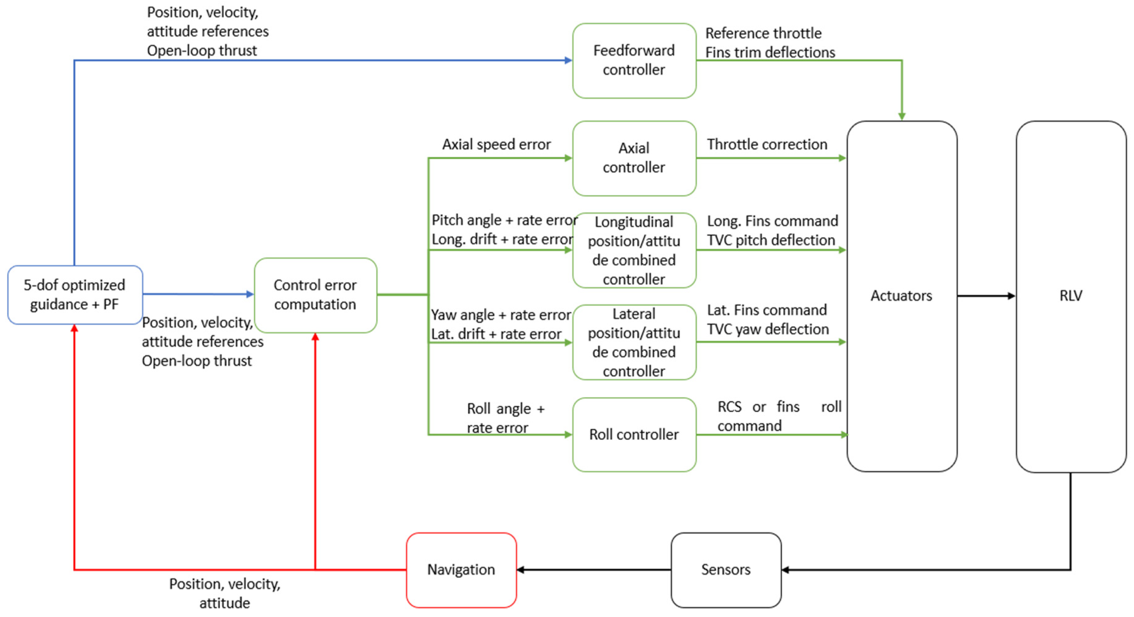
4.4.3. Landing Powered Control Design

The structure for the controller of the landing phase is like the one developed for re-entry. Indeed, fins are preferred over RCSs to improve the actuation capability of the vehicle, and the pitch control logic is given by

$$\left[\begin{array}{c}{\beta }_{\theta }\\ {\delta }_{f,\theta }\end{array}\right]=\left[\begin{array}{cccc}{K}_{\theta }& K_z& K_q& K_{\dot{z}}\\ H_{\theta }& H_z& H_q& H_{\dot{z}}\end{array}\right]\left[\begin{array}{c}{\theta }_e\\ {\mathit{r}}_e\left(3\right)\\ q_e\\ {\mathit{v}}_e\left(3\right)\end{array}\right].$$

(80)

A feedforward fin command is superimposed to (80) according to the same logic specified in Section 4.3.3. Concerning the axial controller, the main difference with (50) is the inclusion of an integral action to compensate for aerodynamic uncertainties. The axial control law is then

$$T_{h, cmd}=K_{V, p}{\mathit{v}}_e\left(1\right)+\int K_{V,i}{\mathit{v}}_e\left(1\right).$$

(81)

The path-following logic in Section 4.2.4 is also used here to extract the points of the reference trajectory to be tracked. The functional architecture for the landing controller is shown in Figure 18.

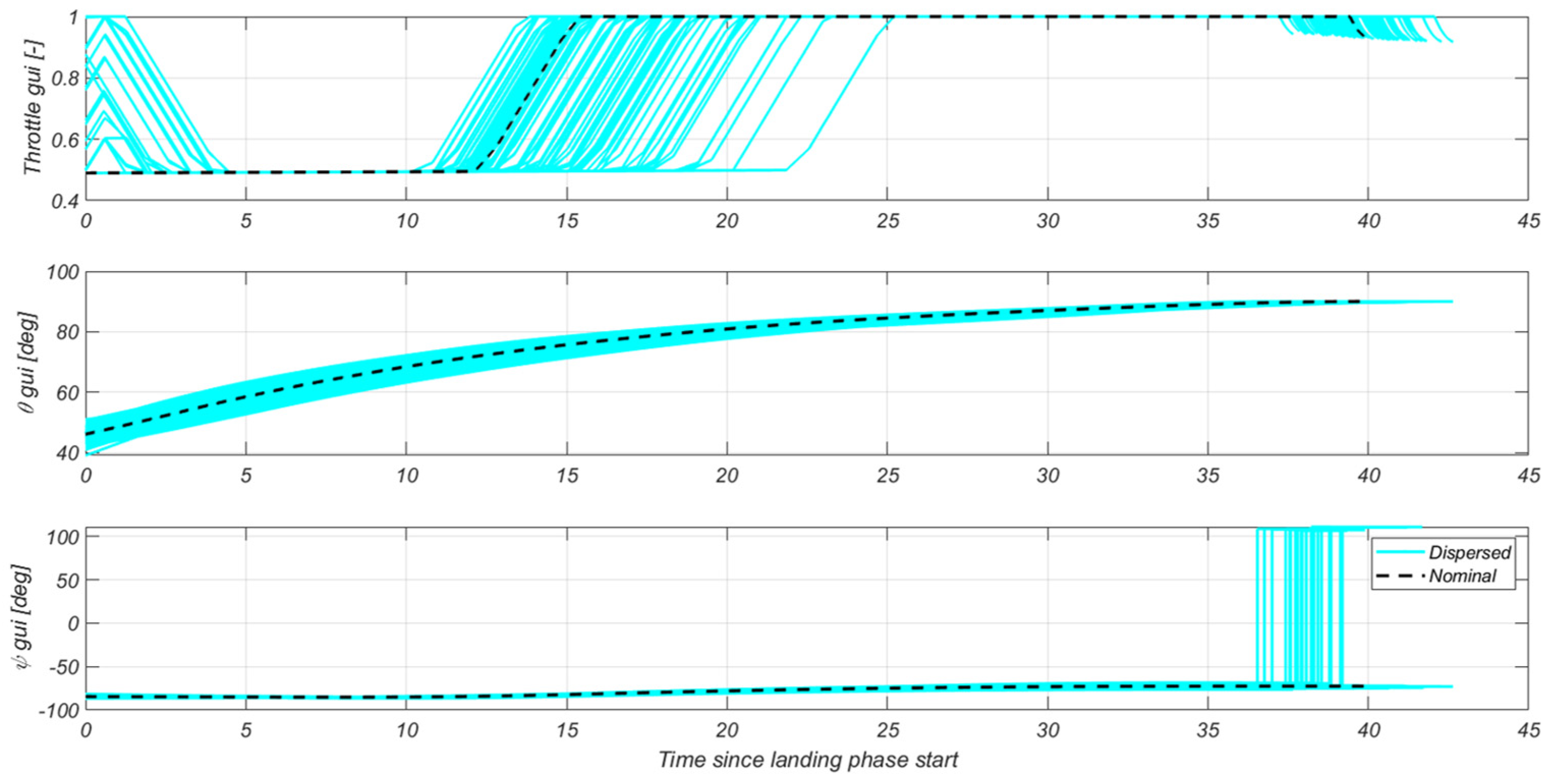
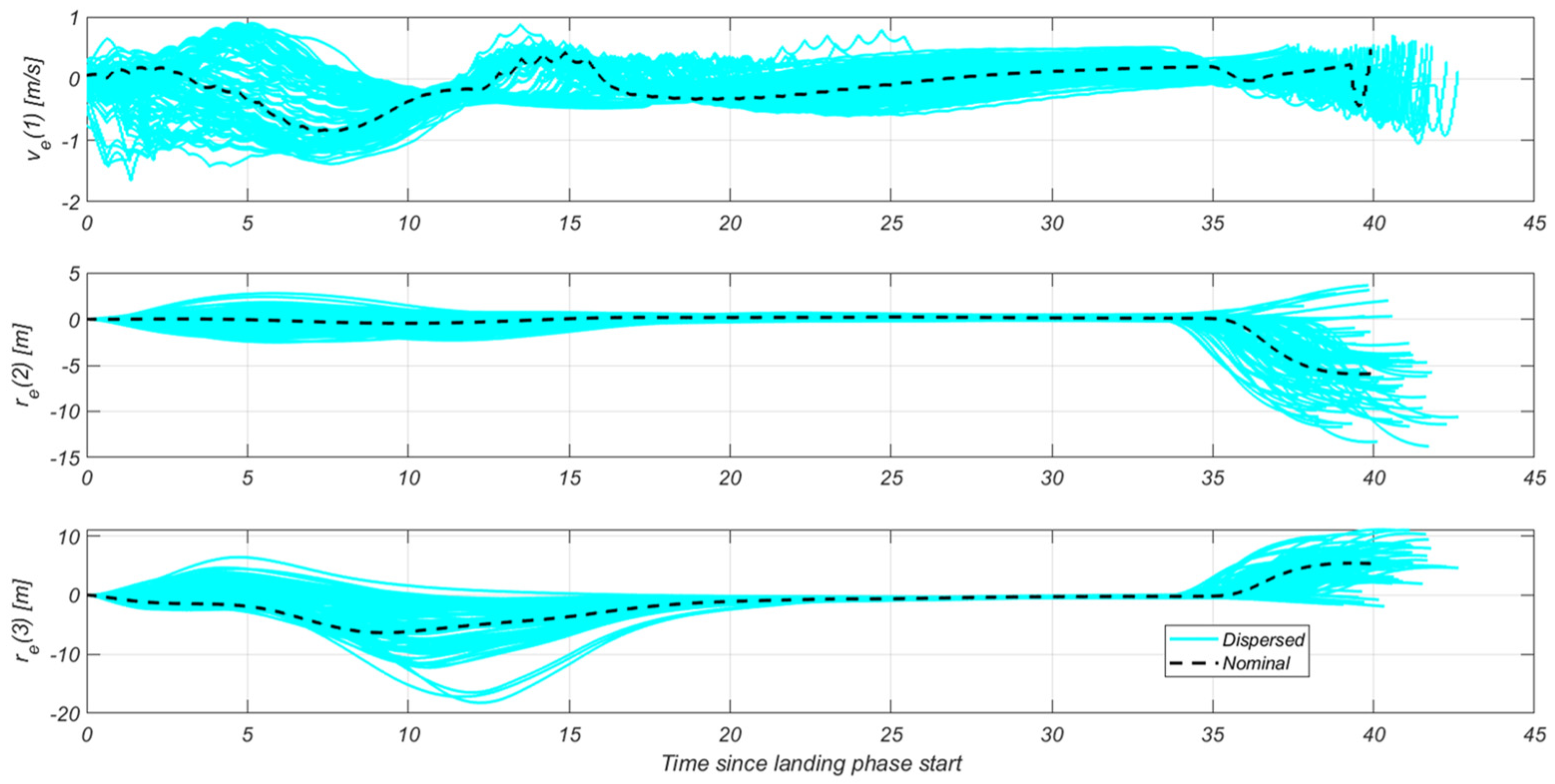
4.4.4. Landing G&C Specific Results

This section reports the main results for the landing phase. The guidance commands are shown in Figure 19. Differently from the re-entry burn scenario, the solutions achieved considering dispersed cases are more regular. For the nominal one, the throttle time history converges to a min–max profile. When dispersions are considered, for some cases, the guidance converges to the same profile with a different switching instant; for other cases, it converges to a max–min–max-like solution. The vehicle orientation is changed to generate the aerodynamic forces necessary to vertically land on the desired point.

The tracking errors are shown in Figure 20. After an initial transient, the vehicle starts moving along the desired path (i.e., ${\mathit{r}}_e\left(2\right), {\mathit{r}}_e\left(3\right), {\mathit{v}}_e\left(1\right)\to 0$). However, due to the uncertainties in aerodynamics and wind, the vehicle needs to change its attitude to follow the desired path. This attitude drift is shown in Figure 21. In the final leg of the flight, the controller gains in (80) are scheduled to reorient the vehicle attitude to land vertically with almost zero lateral velocity. This induces a drift from the nominal path, as shown in Figure 20 (${\mathit{r}}_e\left(2\right), {\mathit{r}}_e\left(3\right)$ plots).

5. Robustness Analysis Results

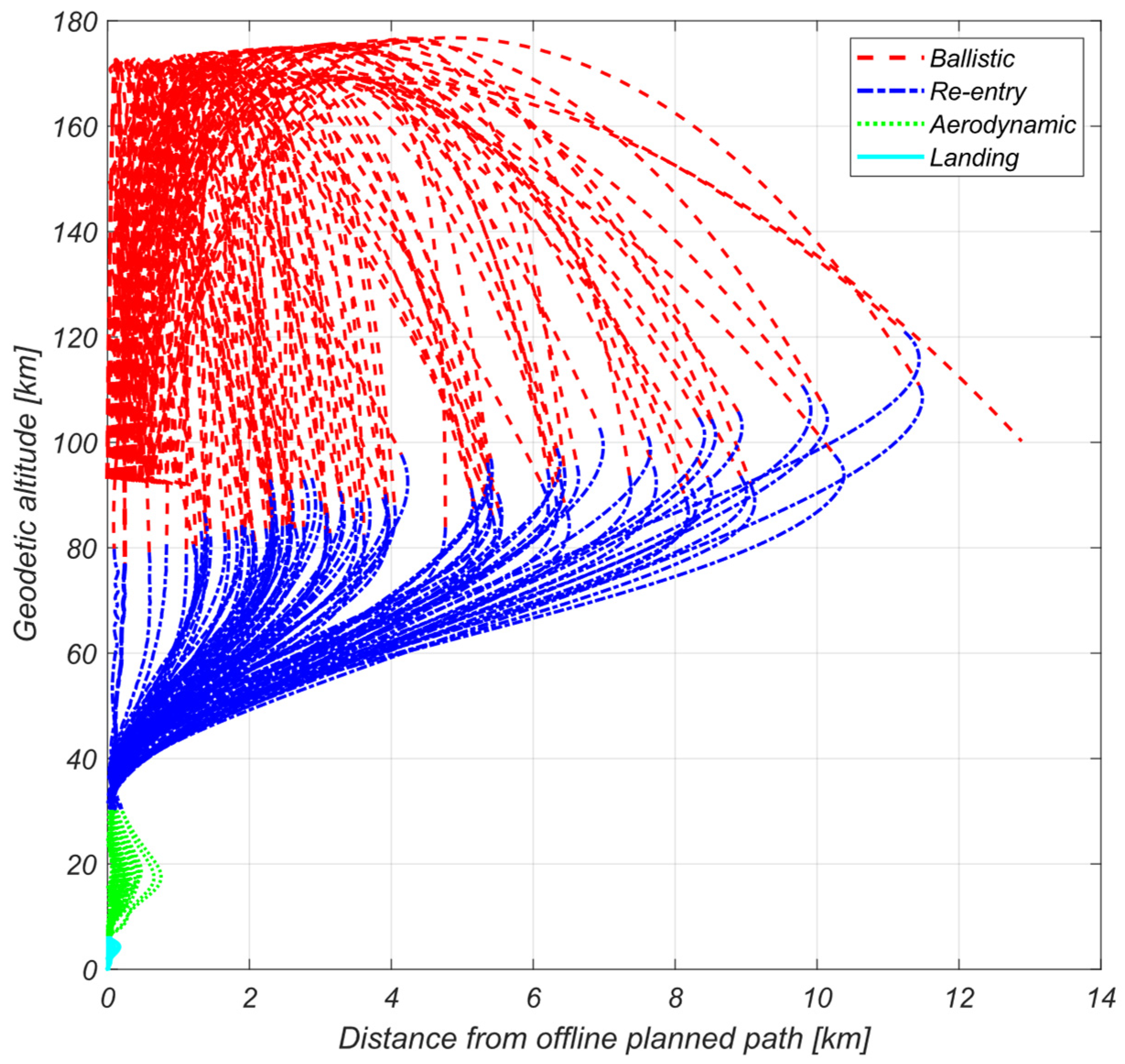
5.1. Scenario Description

This section reports and comments the results of the robustness analysis of the proposed GNC solution. This is tested for a downrange landing scenario from the MECO conditions to the touchdown for RETALT1 and includes all the algorithms and features discussed in Section 4. The main physical parameters of the vehicle are given in Section 2. The effectiveness of the GNC design is assessed with a Monte-Carlo campaign, through a high-fidelity Functional Engineering Simulator (FES), which includes a J2-perturbed gravity model, aerodynamics, wind model, engine model, and 6DoF plant model (see [21]). Other effects like flexible modes and sloshing are not considered in this work, but they will be the subject of future development.

The Monte-Carlo campaign employs several dispersions, including the initial condition at MECO, the atmospheric model and winds, vehicle MCI properties, and aerodynamics coefficients. Concerning the analysis presented in this work, only dispersion on the axial aerodynamics coefficient is considered; however, future work envisions the integration of uncertainties on all the aerodynamic coefficients. Two batches of 100 runs are performed with increasing uncertainty related to the axial coefficients, such that it has a uniform distribution with an error of 10% for the first batch, and 20% for the second one [2,42,43]. Concerning the initial conditions, normal dispersions of $\pm 3\sigma$ are considered with standard deviation, as reported in Table 1. For the MCI, typical uniform dispersions of CoG are used, with a displacement of $\pm 1$ m in the vertical direction (x) and $\pm 0.1$ m in the horizontal ones (y and z). The inertia of the vehicle is, also, affected by uncertainty according to the vehicle characteristic [2]. Regarding the atmospheric parameters and wind, dispersions follow the uncertainties profile according to the models used [41,44].

Table 6. Uncertainty definitions considered within the robustness analysis.

Variables	Distribution	References
Initial conditions	Gaussian	Table 1 [4]
MCI	Uniform	[2]
Aerodynamic database	Uniform	[2,42,43]
Atmospheric parameters	Gaussian	[44]
Winds	Gaussian	[41]

summarizes the uncertainties used for the robustness analysis.

For the analysis performed, Table 5 reports the landing requirements that are considered to deem a Monte-Carlo shot either successful or not:

5.2. Results

Figure 22 shows the distance of the vehicle with respect to the reference trajectory of the mission (i.e., planned during mission analysis studies and used to generate the waypoints in Table 2) as a function of the altitude. As the mission begins (MECO), the vehicle starts accumulating drift with respect to the reference (red lines). This drift is compensated during the re-entry phase; from the figure, it can be seen that the higher the accumulated drift, the higher the altitude at which the burn is triggered. The re-entry burn (blue lines) allows for targeting the desired waypoint with good accuracy, and it almost cancels out the effects of the uncertainties at MECO. The aerodynamic leg (green lines) increases the dispersion cloud (especially in the max Q region); during the landing phase (cyan line), the vehicle converges to the desired flight path as the altitude decreases. This error pattern is compliant with data available in the literature [45] for existing vehicles. This analysis considers the first Monte-Carlo batch, and it presents a success rate of 99 cases over 100. The outlier is visible in the right part of Figure 22, and it highlights the failure on the re-entry guidance.

Figure 23 reports the landing accuracy results and the associated statistics for the same batch of Monte-Carlo runs. In particular, Figure 23a shows the position dispersion with respect to the target, with the associated velocity at touchdown. The circle defines a radial distance from the target of 15 m (green), 20 m (yellow), and 25 m (red). The results show that the GNC can handle the considered dispersions and perform a precise pinpoint landing within the prescribed requirements, featuring accurate and precise performance in position. Also, considering the statistics reported in Figure 23b, it can be noted that both the in-plane velocity and the vertical one are well below the requirements. This demonstrates that the proposed GNC is a promising solution for the problem analyzed.

Concerning the second batch of results, Figure 24 presents the simulations where the uncertainty in the axial coefficient is doubled. As expected, for this scenario, the performance is slightly degraded. Specifically, Figure 24a shows that the GNC achieves good position accuracy, with 95 cases meeting the landing position requirements. However, in seven cases, the touchdown velocity exceeds the prescribed limits (circles with red edge). Furthermore, one case fulfills neither the position nor the velocity requirements (plus four outliers not reported in the figure). This behavior can also be seen in Figure 24b. Despite this, the results of this scenario show similar performance to the previous one, highlighting the robustness of the proposed GNC.

Regarding the unsuccessful Monte-Carlo shots, a dedicated analysis is carried out to identify the possible causes. Figure 25 reports the dispersed trajectories in the altitude–velocity plane for the aerodynamic descent and the landing burn phases. The figure shows in red the trajectories that do not match the landing requirements. It can be noted that the failures are placed at the lower and the upper bounds of the population, where the trajectories are characterized by either relatively high or low velocity at the aerodynamic–landing burn interface. Next phases of the project will focus on the enlargement of the success landing area in the altitude–velocity plane. An adaptive ignition altitude between aero-landing phases could be a promising solution.

The simulations were performed in MIL on an Intel^® Core^TM i7-870H processor with 16.0 GB of RAM. Using this hardware, the performance of the guidance algorithm is very promising, requiring less than a second to obtain a solution when the online guidance is invoked in a nominal scenario. However, as reported in Section 3.4, no further details are given, since real-time performance on a space-rated processor will be an object of investigation for future steps of the project, where SIL and PIL tests will be performed.

6. Conclusions and Future Developments

This paper aims at presenting an end-to-end GNC solution for recovery of a reusable first stage by means of a vertical landing. In particular, this work presents definitions of the guidance and the control methodologies employed for each phase of the mission, describing the main algorithms and strategies and the design choices taken. Concerning the high-altitude ballistic arc, this paper discusses the guidance developed for the flip-over maneuver, as well as adaptive logic to schedule the initial ignition altitude and attitude for the re-entry burn to compensate the dispersions accumulated along the ballistic arc. Moreover, the modeling of the control is provided. For what concerns the guidance of the atmospheric phases, an SCP algorithm is used to compute a reference trajectory onboard depending on the current flight conditions. For each phase, a different formulation of the guidance problem is provided, explaining the assumptions made and the modeling choices. In the re-entry burn phase, particular attention is given to the convexification of the problem, underlying the steps followed. Since the strategy is similar for the aerodynamic descent and the landing burn, only the peculiarities are highlighted, i.e., the benefits obtained with the inclusion of the winds profile in the guidance scheme of the landing burn. For all the phases, the control logic is presented by providing an extensive formulation of the control problem depending on the objective to pursue. For each case, the guidance open-loop commands and the control tracking performance are reported.

The proposed GNC is tested in an end-to-end downrange landing scenario with RETALT1 as reference vehicle by assessing its robustness through two sets of Monte-Carlo campaigns with increasing aerodynamic uncertainties. Strict pinpoint landing requirements are considered for both the position and the velocity. The results demonstrate the robustness of the proposed GNC within the considered uncertainties range by showing the distance error with respect the reference trajectory and the landing performance. In total, 99 cases successfully fulfil the landing requirements for what concerns the first batch of the Monte-Carlo campaign, while for the second, the success cases reduce to 88. For this last scenario, the position landing requirements are met, while experiencing higher touchdown velocity. A preliminary analysis of the outliers is given, and a possible solution is proposed to improve the results. In particular, the following steps will consist in improving the guidance solution by exploiting a different integration scheme for the dynamics constraints [12]. In addition, a more general formulation to handle the initial dispersions at MECO can be highly beneficial for improving the mission success [46].

The proposed GNC obtained interesting and promising results; nevertheless, the following future developments are foreseen to improve the robustness and the capability of the GNC solution. In particular, the next steps of the development of this GNC solution in the context of SALTO include a tailoring to the FL configuration and scenarios and a model-in-the-loop (MIL) test campaign. In addition, the GNC will also be tailored to the T3 configuration and scenario, with the added goal of increasing the test effort to perform SIL and PIL testing to assess the GNC performance for the suborbital flight test scenario.

References

1. de Mirand, A.P.; Bahu, J.M.; Gogdet, O. Ariane Next, a vision for the next generation of Ariane Launcher. Acta Astronaut. 2020, 170, 735–749. [Google Scholar] [CrossRef]
2. Marwege, A.; Gülhan, A.; Klevansky, J.; Hantz, C.; Karl, S.; Laureti, M.; De Zaiacomo, G.; Vos, J.; Jevons, M.; Thies, C.; et al. RETALT: Review of technologies and overview of design changes. CEAS Space J. 2022, 14, 433–445. [Google Scholar] [CrossRef] [PubMed]
3. SALTO-reuSable strAtegic Space Launcher Technologies & Operations, Salto Consortium Associated Partners. Available online: https://salto-project.eu/ (accessed on 6 April 2025).
4. De Zaiacomo, G.; Arnao, G.B.; Bund, R.; Bonetti, D. Mission engineering for the RETALT VTVL launcher. CEAS Space J. 2022, 14, 533–549. [Google Scholar] [CrossRef]
5. Guadagnini, J.; Lavagna, M.; Rosa, P. Model predictive control for reusable space launcher guidance improvement. Acta Astronaut. 2022, 193, 767–778. [Google Scholar] [CrossRef]
6. Szmuk, M.; Reynolds, T.P.; Acikmese, B. Successive Convexification for Real-Time Six-Degree-of-Freedom Powered Descent Guidance with State-Triggered Constraints. J. Guid. Control Dyn. 2020, 43, 1399–1413. [Google Scholar] [CrossRef]
7. Malyuta, D.; Reynolds, T.; Szmuk, M.; Lew, T.; Bonalli, R.; Pavone, M.; Açıkmeşe, B. Convex Optimization for Trajectory Generation. IEEE Control Syst. Mag. 2022, 42, 20–113. [Google Scholar] [CrossRef]
8. Mao, Y.; Szmuk, M.; Acikmese, B. Successive convexification of non-convex optimal control problems and its convergence properties. In Proceedings of the IEEE 55th Conference on Decision and Control (CDC), Las Vegas, NV, USA, 12–14 December 2016. [Google Scholar] [CrossRef]
9. Wang, J.; Cui, N.; Wei, C. Optimal Rocket Landing Guidance Using Convex Optimization and Model Predictive Control. J. Guid. Control Dyn. 2019, 42, 1078–1092. [Google Scholar] [CrossRef]
10. Simplicio, P. Guidance and Control Elements for Improved Access to Space from Planetary Landers to Reusable Launchers. Ph.D. Thesis, University of Bristol, Department of Aerospace Engineering, Bristol, UK, November 2019. [Google Scholar]
11. Szmuk, M.; Acikmese, B. Successive Convexification for 6-DoF Mars Rocket Powered Landing with Free-Final-Time. In Proceedings of the 2018 AIAA Guidance, Navigation and Control Conference, Kissimmee, FL, USA, 8–12 January 2018. [Google Scholar] [CrossRef]
12. Malyuta, D.; Reynolds, T.; Szmuk, M.; Mesbahi, M.; Acikmese, B.; Carson, J.M. Discretization Performance and Accuracy Analysis for the Rocket Powered Descent Guidance Problem. In Proceedings of the AIAA SCITECH 2019 Forum, San Diego, CA, USA, 7–11 January 2019. [Google Scholar] [CrossRef]
13. Sagliano, M.; Heidecker, A.; Hernández, J.M.; Farí, S.; Schlottere, M.; Woicke, S.; Seelbinder, D.; Dumont, E. Onboard Guidance for Reusable Rockets: Aerodynamic Descent and Powered Landing. In Proceedings of the AIAA Scitech 2021 Forum, Virtual Event, Orlando, FL, USA, 11–21 January 2021. [Google Scholar] [CrossRef]
14. Bucchioni, G.; Innocenti, M. Rendezvous in Cis-Lunar Space near Rectilinear Halo Orbit: Dynamics and Control Issues Aerospace. Aerospace 2021, 8, 68. [Google Scholar] [CrossRef]
15. Mooij, E. Linear Quadratic Regulator Design for an Unpowered, Winged Re-Entry Vehicle; Delft University Press: Delft, The Netherlands, 1997. [Google Scholar]
16. Lu, P. Regulation About Time-Varying Trajectories: Precision Entry Guidance Illustrated in Guidance. In Proceedings of the Navigation, and Control Conference and Exhibit, Portland, OR, USA, 9–11 August 1999. [Google Scholar] [CrossRef]
17. Pascucci, C.A.; Bennani, S.; Bemporad, A. Model predictive control for powered descent guidance and control. In Proceedings of the 2015 European Control Conference (ECC), Linz, Austria, 12–15 June 2015. [Google Scholar] [CrossRef]
18. Jung, Y.; Bang, H. Mars precision landing guidance based on model predictive control approach. Proc. Inst. Mech. Eng. 2015, 230, 2048–2062. [Google Scholar] [CrossRef]
19. Sagliano, M.; Tsukamoto, T.; Ishimoto, S.; Farì, S.; Dumont, E.; Seelbinder, D.; Schlotterer, M.; Heidecker, A.; Macés-Hernández, J.A.; Woicke, S. Robust Control for reusable rockets via structured H-infinity Synthesis. In Proceedings of the ESA GNC 2021, Virtual, 22–25 June 2021. [Google Scholar]
20. Sagliano, M.; Macés, A.J.H.; Farí, S.; Heidecker, A.; Schlotterer, M.; Woicke, S.; Seelbinder, D.; Krummen, S.; Dumont, E. Unified-Loop Structured H-Infinity Control for Aerodynamic Steering of Reusable Rockets. J. Guid. Control Dyn. 2023, 46, 815–837. [Google Scholar] [CrossRef]
21. Ghignoni, P.; Botelho, A.; Recupero, C.; Fernandez, V.; Fabrizi, A.; De Zaiacomo, G. RETALT: Recovery GNC for the Retro-Propulsive Vertical Landing of an Orbital Launch Vehicle. In Proceedings of the 2nd International Conference on High-Speed Vehicle 1227 Science Technology, Bruges, Belgium, 11–16 September 2022. [Google Scholar] [CrossRef]
22. Vandersteen, J.; Bennani, S.; Roux, C. Robust Rocket Navigation with Sensor Uncertainties: Vega Launcher Application. J. Spacecr. Rocket. 2018, 55, 153–166. [Google Scholar] [CrossRef]
23. Spada, F.; Ghignoni, P.; Botelho, A.; De Zaiacomo, G.; Rosa, P. Successive Convexification-based Fuel-Optimal High-Altitude Guidance of the RETALT Reusable Launcher. In Proceedings of the ESA 12th International Conference on Guidance Navigation and Control and 9th International Conference on Astrodynamics Tools and Techniques, Sopot, Poland, 12–16 June 2023. [Google Scholar] [CrossRef]
24. Reynolds, T.; Malyuta, D.; Mesbahi, M.; Acikmese, B.; Carson, J.M. A Real-Time Algorithm for Non-Convex Powered Descent Guidance In Proceedings of the AIAA Scitech 2020 Forum, Orlando, FL, USA, 6–10 January 2020. [CrossRef]
25. Andersson, J.A.E.; Gillis, J.; Horn, G.; Rawlings, J.B.; Diehl, M. CasADi: A software framework for nonlinear optimization and optimal control. Math. Program. Comput. 2019, 11, 1–36. [Google Scholar] [CrossRef]
26. Domahidi, A.; Chu, E.; Boyd, S. ECOS: An SOCP solver for embedded systems. In Proceedings of the European Control Conference (ECC), Zurich, Switzerland, 17–19 July 2013. [Google Scholar] [CrossRef]
27. Apkarian, P.; Noll, D. Nonsmooth H-infinity Synthesis. IEEE Trans. Autom. Control 2006, 51, 71–86. [Google Scholar] [CrossRef]
28. Apkarian, P.; Gahinet, P.; Buhr, C. Multi-model, multi-objective tuning of fixed-structure controllers. In Proceedings of the European Control Conference (ECC), Strasbourg, France, 24–27 June 2014. [Google Scholar] [CrossRef]
29. Simplicio, P.; Bennani, S.; Marcos, A.; Roux, C.; Lefort, X. Structured Singular-Value Analysis of the Vega Launcher in Atmospheric Flight. J. Guid. Control Dynamcis 2016, 39, 1342–1355. [Google Scholar] [CrossRef]
30. De Zaiacomo, G.; Medici, G.; Princi, A.; Ghignoni, P.; Botelho, A.; Arlandis, M.M.; Recupero, C.; Fabrizi, A.; Fernandez, V.; Guidotti, G. RETALT: Development of Key Flight Dynamics and GNC Technologies for Reusable Launchers. In Proceedings of the 73rd International Astronautical Congress (IAC), Paris, France, 18–22 September 2022. [Google Scholar] [CrossRef]
31. De Oliveira, A.M.A. Guidance and Control System Design for Reusable Launch Vehicle Descent and Precise Landing. Ph.D. Thesis, Politecnico di Milano, Milano, Italy, 2024. [Google Scholar]
32. Watcher, A.; Biegler, L.T. On the Implementation of an Interior-Point Filter Line-Search Algorithm for Large-Scale Nonlinear Programming. Math. Program. 2006, 106, 25–57. [Google Scholar] [CrossRef]
33. Spada, F.; Sagliano, M.; Topputo, F. Direct-Indirect Hybrid Strategy for Optimal Powered Descent and Landing. J. Spacecr. Rocket. 2023, 60, 1787–1804. [Google Scholar] [CrossRef]
34. Malyuta, D.; Acikmese, B. Fast Homotopy for Spacecraft Rendezvous Trajectory Optimization with Discrete Logic. J. Guid. Control Dyn. 2023, 46, 1262–1279. [Google Scholar] [CrossRef]
35. Landis Markley, F.; Crassidis, J.L. Fundamentals of Spacecraft Attitude Determination and Control, 1st ed.; Springer: Berlin/Heidelberg, Germany, 2014. [Google Scholar]
36. Korzun, A.M.; Cruz, J.R.; Braun, R.D. A Survey of Supersonic Retropropulsion Technology for Mars Entry, Descent, and Landing. In Proceedings of the IEEE Aerospace, Big Sky, MT, USA, 1–8 March 2008. [Google Scholar] [CrossRef]
37. Brendel, E.; Hérissé, B.; Bourgeois, E. Optimal guidance for toss back concepts of Reusable Launch Vehicles. In Proceedings of the 8th European Conference for Aeronautics and Aerospace Sciences (EUCASS), Madrid, Spain, 1–4 July 2019. [Google Scholar]
38. Navarro-Tapia, D. Robust and Adaptive TVC Control Design Approaches for the VEGA Launcher. Ph.D. Thesis, University of Bristol, Bristol, UK, 2019. [Google Scholar]
39. Cunha, R.; Duarte, A.; Gomes, P.; Silvestre, C. A Path-Following Preview Controller for Autonomous Air Vehicles. In Proceedings of the AIAA Guidance, Navigation, and Control Conference and Exhibit, Keystone, CO, USA, 21–24 August 2006. [Google Scholar]
40. Mathematics, E.O. The European Mathematical Society. Available online: http://encyclopediaofmath.org/index.php?title=Cardano_formula&oldid=29227 (accessed on 9 January 2025).
41. Horizontal Wind Model 14 Website U.S. Naval Research Laboratory. Available online: https://map.nrl.navy.mil/map/pub/nrl/HWM/HWM14/ (accessed on 31 January 2024).
42. Charbonnier, D.; Vos, J.B.; Marwege, A.; Hantz, C. Computational fluid dynamics investigations of aerodynamic control surfaces of a vertical landing configuration. CEAS Space J. 2022, 14, 1–16. [Google Scholar] [CrossRef]
43. Marwege, A.; Hantz, C.; Kirchheck, D.; Klevanski, J.; Gulhan, A.; Charbonnier, D.; Von, J.B. Wind tunnel experiments of interstage segments used for aerodynamic control of retro-propulsion assisted landing vehicles. CEAS Space J. 2022, 14, 447–471. [Google Scholar] [CrossRef]
44. NRLMSIS-00 Atmospheric Model Community Coordinated Modeling Center Website. Available online: https://ccmc.gsfc.nasa.gov/models/NRLMSIS~00/ (accessed on 31 January 2024).
45. Blackmore, L. Autonomous precision landing of space rockets. Bridge 2016, 4, 15–20. [Google Scholar]
46. Kamath, A.G.; Elango, P.; Yu, Y.; Mceowen, S.; Chari, G.M.; Carson, J.M., III; Acikmese, B. Real-Time Sequential Conic Optimization for Multi-Phase Rocket Landing Guidance. IFAC-PapersOnLine 2023, 56, 3118–3125. [Google Scholar] [CrossRef]
Figure 1. Downrange landing reference mission main phases.
Aerospace 12 00339 g001
Figure 2. GNC functional architecture.
Aerospace 12 00339 g002
Figure 3. Block diagram of the offline pre-parser and online parser. In this case, the online parser is an emulator of the actual onboard software that can be exploited during the preliminary tuning and guidance design.
Aerospace 12 00339 g003
Figure 4. Standard setup for controller synthesis.
Aerospace 12 00339 g004
Figure 5. Procedure employed to generate the online guidance coherent LUTs.
Aerospace 12 00339 g005
Figure 6. Sensitivity analysis of the number of CVX iterations needed to solve the 3DoF PDG problem (top) and the 5DoF fuel-optimal re-entry problem (bottom).
Aerospace 12 00339 g006aAerospace 12 00339 g006b
Figure 7. Attitude tracking error.
Aerospace 12 00339 g007
Figure 8. Re-entry controller (in green) functional architecture.
Aerospace 12 00339 g008
Figure 9. Path-following approach principles.
Aerospace 12 00339 g009
Figure 10. Computation of the closest intervals. Closest node to actual location (star) in green.
Aerospace 12 00339 g010
Figure 11. Guidance open-loop commands for re-entry.
Aerospace 12 00339 g011
Figure 12. Control tracking errors for re-entry phase.
Aerospace 12 00339 g012
Figure 13. Aerodynamic controller (in green) functional architecture.
Aerospace 12 00339 g013
Figure 14. Guidance open-loop commands for aerodynamic phase.
Aerospace 12 00339 g014
Figure 15. Control tracking errors for aerodynamic phase.
Aerospace 12 00339 g015
Figure 18. Landing controller (in green) functional architecture.
Aerospace 12 00339 g018
Figure 19. Guidance open-loop commands for landing phase.
Aerospace 12 00339 g019
Figure 20. Control tracking errors for landing phase.
Aerospace 12 00339 g020
Figure 21. Control attitude error for landing phase.
Aerospace 12 00339 g021
Figure 22. Vehicle distance from the desired mission path as a function of altitude for the different flight phases.
Aerospace 12 00339 g022
Figure 23. Landing accuracy (a) and landing statistics (b) for the end-to-end scenario for the first Monte-Carlo batch.
Aerospace 12 00339 g023
Figure 24. Landing accuracy (a) and landing statistics (b) for the end-to-end scenario for the second Monte-Carlo batch.
Aerospace 12 00339 g024
Figure 25. Aero-propulsive trajectory dispersions.
Aerospace 12 00339 g025