Fault-Tolerant Dynamic Allocation Strategies for Launcher Systems

Abstract

This article presents fault-tolerant dynamic allocation strategies designed to mitigate propulsion and actuation failures in launch vehicles using a clustered engine configuration. In particular, it addresses engine thrust loss and thrust vector control (TVC) jamming faults during the atmospheric ascent flight of a five-engine launch vehicle. Three different strategies are introduced: a fault-tolerant pseudo-inverse solution, a convex optimization-based approach, and a constrained nonlinear optimization one. These approaches are analyzed and compared at a linear design point and further evaluated using a nonlinear simulator of the launcher. The results demonstrate that these three dynamic allocation techniques are able to provide successful recovery from engine thrust loss failures (up to a certain level depending on the engine throttling capability), TVC actuator jamming failures, and simultaneous engine and actuator failures.

1. Introduction

The adoption of clustered rocket engines (CREs) is making a significant impact on the reusable launch market due to their several advantages. Compared to traditional single-engine launchers, CRE configurations offer higher thrust and enhanced robustness due to their combined power and hardware-redundant nature. They also enable lighter and less complex engine and actuator subsystems by distributing thrust and loads more efficiently. Additionally, they result in reduced costs, particularly when manufacturers leverage advanced production techniques such as serial 3D printing to fabricate simpler, cluster-compatible engines. Beyond these benefits, CRE configurations play a crucial role in advancing new mission capabilities, including vertical landing for reusability and increased launch frequency to meet the existing growing demand in the satellite market—both of which require enhanced safety in launch systems.

Most mission failures in the last 25 years resulted from propulsion failures (50%), followed by guidance, navigation, and control (GNC) issues (15%, which includes actuator failures), and separation problems (5%) [1]. Currently, European launch vehicles rely primarily on passive fault diagnosis and recovery strategies, with limited adoption of active fault detection, isolation, and reconfiguration (FDIR) techniques, mostly implemented through ad hoc solutions. In contrast, the American launch market has demonstrated that CRE configurations provide propulsion and actuation hardware redundancy, paving the way for more reliable and smarter missions. For instance, the Falcon 9 successfully reached its target orbit in March 2020 despite losing one of the nine first-stage engines. Additionally, recently in June 2024, the Starship launch vehicle lost one engine shortly after launch but still achieved its planned orbit.

In line with the general increased need for performance and safety for launch systems, and the increased complexity at the system level of CRE configurations, more advanced FDIR methods are required than those currently used for European launchers. However, research studies on advanced FDIR techniques for launch vehicles in Europe have not progressed as much as those performed in other fields such as aviation, where significant progress has been achieved through European programs like ADDSAFE [2], RECONFIGURE [3], and VISION [4]. Some exceptions in the European space sector include studies on fault detection and isolation (FDI) for a Vulcain-2 like rocket engine [5,6], optimization-based thrust vector control (TVC) allocation for actuator failures [7], and robust FDI algorithms for launch vehicle TVC systems [8].

More recently, the European Space Agency (ESA) initiated the project “Fault-Tolerant Control of Clusters of Rocket Engines” (FTC-CRE), aimed at developing system-level fault-tolerant control (FTC) strategies for launch vehicles. FTC-CRE was participated in by GMV, responsible for the launch vehicle simulator (supported by TASC) and guidance-based reconfiguration; SABCA, responsible for the TVC actuator modeling; and TASC, which led the development of dynamic allocation and control reconfiguration schemes.

Within FTC-CRE, four reconfiguration schemes were developed: (1) dynamic allocation, (2) control reconfiguration, (3) TVC reconfiguration, and (4) guidance reconfiguration. This article focuses on the first reconfiguration scheme, which replaces the nominal allocation function with a fault-tolerant dynamic allocation function designed to recover from propulsion and actuation failures. The control reconfiguration strategy is introduced in [9], while Refs. [10,11] present Monte Carlo campaign results for all the reconfiguration schemes.

The layout of this article is as follows. Section 2 introduces the launch vehicle use case, detailing the derivation of engine force and moment equations, and the simulation environment. Section 3 presents various dynamic allocation schemes, which are evaluated in Section 4 for a linear operating point at maximum dynamic pressure, and then further assessed using a nonlinear launch vehicle simulator in Section 5. Finally, conclusions are given in Section 6.

2. Ascent-Flight Launcher Benchmark

2.1. Launch Vehicle Description

The case study focuses on a two-stage launch vehicle measuring approximately 25 m in length and 1.8 m in diameter, with a gross lift-off mass of nearly 33,000 kg. The vehicle carries a 250 kg of payload and follows a trajectory from the Guiana Space Center to a Sun Synchronous Orbit at an altitude of 400 km.

The first stage is powered by a cluster of five liquid propulsion engines arranged in a cross-shaped configuration, as illustrated in Figure 1. The central engine is fixed, while each of the four outer engines is equipped with two TVC actuators. The engines operate within a throttling range of 30–110%, providing the necessary flexibility for mission adaptability.

In addition to the standard attitude and lateral deviation requirements, the case study considers two additional specifications. First, the aerodynamic load indicator, $Q\alpha$, must remain below 80 kPa° to prevent severe aerodynamic forces impacting the launcher. Second, the roll rate must be kept lower than 5 °/s to ensure that the pitch and yaw attitude control channels remain effectively decoupled form the roll dynamics.

2.2. Derivation of Engine Force and Moment Equations

In preparation for the application of dynamic allocation techniques, this section derives the equations governing the engine forces and moments acting on the launch vehicle.

For each engine, the forces in the TVC reference frame can be computed as follows:

$${\mathbf{F}}_i^{TVC}=\left[\begin{array}{c}{F}_{x_i}^{TVC}\\ F_{y_i}^{TVC}\\ F_{z_i}^{TVC}\end{array}\right]=T_i\left[\begin{array}{c}sin{\delta }_{i,B}\\ -sin{\delta }_{i,A}cos{\delta }_{i,B}\\ cos{\delta }_{i,A}cos{\delta }_{i,B}\end{array}\right]$$

(1)

where $T_i$ is the engine thrust, and ${\delta }_{i,A}$ and ${\delta }_{i,B}$ are the TVC deflections in the TVC reference frame, see Figure 1.

The body-frame forces can be computed from Equation (1) using the following frame transformation:

$${\mathbf{F}}_i^{BF}=\left[\begin{array}{c}{F}_{x_i}^{BF}\\ F_{y_i}^{BF}\\ F_{z_i}^{BF}\end{array}\right]=\left[\begin{array}{c}{\displaystyle \frac{\sqrt{2}}{2}}(F_{x_i}^{TVC}+F_{y_i}^{TVC})\\ -{\displaystyle \frac{\sqrt{2}}{2}}(F_{x_i}^{TVC}-F_{y_i}^{TVC})\\ F_{z_i}^{TVC}\end{array}\right]=T_i\left[\begin{array}{c}{\displaystyle \frac{\sqrt{2}}{2}}(sin{\delta }_{i,B}-sin{\delta }_{i,A}cos{\delta }_{i,B})\\ -{\displaystyle \frac{\sqrt{2}}{2}}(sin{\delta }_{i,B}+sin{\delta }_{i,A}cos{\delta }_{i,B})\\ cos{\delta }_{i,A}cos{\delta }_{i,B}\end{array}\right]$$

(2)

The torque of each engine is computed using the body-axis engine forces from Equation (2) and the moment arm ${\mathbf{r}}_i={\left[\begin{array}{ccc}{x}_i& y_i& z_i\end{array}\right]}^T$ given by the distance from the position of the nozzle pivot point ${\mathbf{r}}_{PVP}$ to the launch vehicle center of mass ${\mathbf{r}}_{CoM}$:

$${\mathbf{M}}_i^{BF}=({\mathbf{r}}_{PVP}-{\mathbf{r}}_{CoM})\times {\mathbf{F}}_i^{BF}=\left[\begin{array}{c}{x}_i\\ y_i\\ z_i\end{array}\right]\times {\mathbf{F}}_i^{BF}=\left[\begin{array}{c}{y}_i{F}_{z_i}^{BF}-z_i{F}_{y_i}^{BF}\\ z_i{F}_{x_i}^{BF}-x_i{F}_{z_i}^{BF}\\ x_i{F}_{y_i}^{BF}-y_i{F}_{x_i}^{BF}\end{array}\right]$$

(3)

Equations (2) and (3) can be combined together to express the engine moments as an expression of thrust ($T_i$), cluster geometry ($x_i$, $y_i$ and $z_i$), and gimbal deflections (${\delta }_{i,A}$ and ${\delta }_{i,B}$) as shown in Equation (4).

$${\mathbf{M}}_i^{BF}=T_i\left[\begin{array}{c}{y}_{i}cos{\delta }_{i,A}cos{\delta }_{i,B}+{\displaystyle \frac{\sqrt{2}}{2}}{z}_i(sin{\delta }_{i,B}+sin{\delta }_{i,A}cos{\delta }_{i,B})\\ {\displaystyle \frac{\sqrt{2}}{2}}{z}_i(sin{\delta }_{i,B}-sin{\delta }_{i,A}cos{\delta }_{i,B})-x_{i}cos{\delta }_{i,A}cos{\delta }_{i,B}\\ -{\displaystyle \frac{\sqrt{2}}{2}}{x}_i(sin{\delta }_{i,B}+sin{\delta }_{i,A}cos{\delta }_{i,B})-{\displaystyle \frac{\sqrt{2}}{2}}{y}_i(sin{\delta }_{i,B}-sin{\delta }_{i,A}cos{\delta }_{i,B})\end{array}\right]$$

(4)

The body-axis force and moment equations can be simplified using small angle assumptions as follows:

$${\mathbf{F}}_i^{BF}\approx T_i\left[\begin{array}{c}{\displaystyle \frac{\sqrt{2}}{2}}({\delta }_{i,B}-{\delta }_{i,A})\\ -{\displaystyle \frac{\sqrt{2}}{2}}({\delta }_{i,B}+{\delta }_{i,A})\\ 1\end{array}\right]$$

(5)

$${\mathbf{M}}_i^{BF}\approx T_i\left[\begin{array}{c}{y}_i+{\displaystyle \frac{\sqrt{2}}{2}}{z}_i({\delta }_{i,B}+{\delta }_{i,A})\\ {\displaystyle \frac{\sqrt{2}}{2}}{z}_i({\delta }_{i,B}-{\delta }_{i,A})-x_i\\ -{\displaystyle \frac{\sqrt{2}}{2}}{x}_i({\delta }_{i,B}+{\delta }_{i,A})-{\displaystyle \frac{\sqrt{2}}{2}}{y}_i({\delta }_{i,B}-{\delta }_{i,A})\end{array}\right]$$

(6)

The resulting engine moments and forces are given in Equation (7), where the contributions of each engine are considered and re-arranged in terms of the unknown gimbal deflections ${\delta }_{i,A}$ and ${\delta }_{i,B}$. Note here that the first engine does not generate any moment (i.e., $M_1=0$) since it is positioned at the center of the body-axis frame (i.e., $x_1=y_1=0$) and is not gimbaled (i.e., ${\delta }_{1,A}={\delta }_{1,B}=0$). Additionally, the symmetry of the cluster configuration is taken into consideration, such that $z_1=z_2=z_3=z_4=z_5$, $y_2=y_4=x_3=x_5=0$, $x_2=-x_4$, and $y_3=-y_5$. For simplicity, the superscript BF, indicating the reference frame, is omitted from this point forward.

$$\underset{\mathbf{C}}{\underbrace{\left[\begin{array}{c}{M}_x\\ M_y\\ M_z\\ F_x\\ F_y\\ F_z\end{array}\right]}}=\underset{\mathbf{A}}{\underbrace{{\displaystyle \frac{\sqrt{2}}{2}}\left[\begin{array}{cccccccc}{T}_2{z}_1& T_2{z}_1& T_3{z}_1& T_3{z}_1& T_4{z}_1& T_4{z}_1& T_5{z}_1& T_5{z}_1\\ -T_2{z}_1& T_2{z}_1& -T_3{z}_1& T_3{z}_1& -T_4{z}_1& T_4{z}_1& -T_5{z}_1& T_5{z}_1\\ -T_2{x}_2& -T_2{x}_2& T_3{y}_3& -T_3{y}_3& T_4{x}_2& T_4{x}_2& -T_5{y}_3& T_5{y}_3\\ -T_2& T_2& -T_3& T_3& -T_4& T_4& -T_5& T_5\\ -T_2& -T_2& -T_3& -T_3& -T_4& -T_4& -T_5& -T_5\\ 0& 0& 0& 0& 0& 0& 0& 0\end{array}\right]}}\underset{\mathsf{\Gamma }}{\underbrace{\left[\begin{array}{c}{\delta }_{2,A}\\ {\delta }_{2,B}\\ {\delta }_{3,A}\\ {\delta }_{3,B}\\ {\delta }_{4,A}\\ {\delta }_{4,B}\\ {\delta }_{5,A}\\ {\delta }_{5,B}\end{array}\right]}}+\underset{\mathbf{D}}{\underbrace{\left[\begin{array}{c}{y}_3(T_3-T_5)\\ x_2(T_4-T_2)\\ 0\\ 0\\ 0\\ T_1+T_2+T_3+T_4+T_5\end{array}\right]}}$$

(7)

The solution to Equation (7) is inherently underdetermined, as the number of unknowns (engine thrust levels and TVC actuator deflections) exceeds the number of available equations. Section 2.3.3 introduces the allocation function used in this study to solve Equation (7) under non-faulty conditions. Section 3, on the other hand, presents several dynamic allocation functions designed to address Equation (7) in the presence of engine and/or TVC actuator failures.

For a given allocation solution, (i.e., engine thrust configuration and a TVC deflection vector), let us define the residual $\mathbf{R}$ of the dynamic allocation solution as follows:

$$\mathbf{R}=\mathbf{A} · \mathsf{\Gamma }+\mathbf{D}-\mathbf{C}$$

(8)

2.3. Simulation Environment

The launch vehicle dynamics are simulated in a functional engineering simulator (FES) implemented in Matlab/Simulink. Originally developed by GMV, this nonlinear simulator was later adapted during the FTC-CRE activity to incorporate engine and TVC actuator failures. Key features of the FES include the ability to simulate environmental effects such as wind and turbulence, as well as models for sloshing and navigation performance.

A brief description of the most relevant components is provided below, with further details available in [10,11].

2.3.1. Actuation System

The actuation suite consists of a cluster of engines arranged as shown in Figure 1, along with a set of eight TVC actuators (two per engine). Additionally, a reaction control system (RCS) composed of eight reaction thrusters is employed for roll rate control.

The thrust vector actuation system (TVAS) implemented in the FES corresponds to a high-fidelity model developed by SABCA using Multiphysics Simscape modeling. The model of each electromechanical actuator (EMA) includes the permanent magnet synchronous motor, gearbox, ball screw, power switches, sensors, software controller, and nozzle dynamics. The TVC nominal behavior was validated using real test data from SABCA’s EMAs.

Three types of failures were considered in FTC-CRE and implemented in the FES:

• Engine loss of thrust—modeled as a proportional reduction in the mass flow of both oxidizer and fuel injectors, resulting in a reduction in the total mass flow by a multiplicative factor;
• TVC jamming—modeled as the actuator being stuck at a fixed, non-zero deflection angle;
• TVC loss of power—modeled as the actuator becoming free to move, leading to uncontrolled deflections at its maximum range.

This article focuses on engine thrust loss and TVC jamming failures, while results related to TVC power loss failures are discussed in [11].

2.3.2. GNC FDIR Function

The GNC FDIR function receives telemetry from the engines and TVC actuator health monitoring systems and triggers a reconfiguration in the event of a failure. Within FTC-CRE, four reconfiguration schemes were developed:

• Dynamic allocation;
• Control reconfiguration;
• TVC reconfiguration;
• Guidance reconfiguration.

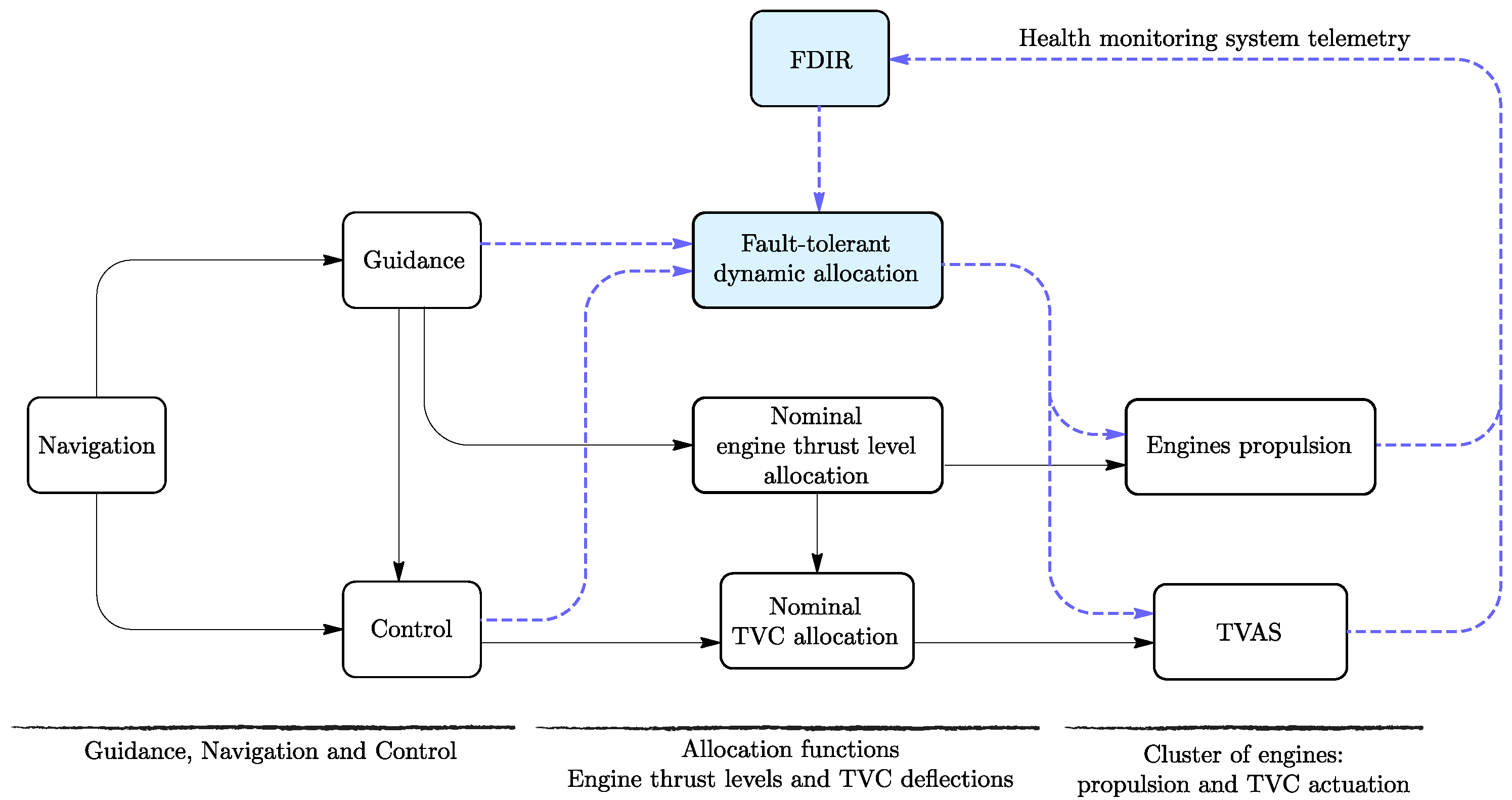
This article focuses on the first reconfiguration scheme, which involves replacing the nominal allocation functions (e.g., engine thrust level and TVC) with a fault-tolerant allocation function. This scheme is illustrated in Figure 2, which depicts the high-level architecture of the simulator for this specific reconfiguration case. As the FTC-CRE activity primarily addressed fault reconfiguration strategies, the fault, detection, and isolation (FDI) function was assumed to be ideal.

2.3.3. Nominal Allocation Function

The nominal allocation function consists of two main modules: a straightforward thrust allocation scheme, and a TVC allocation method, which is based on the high-efficiency quasi-linear algorithm proposed in [12].

The nominal engine thrust allocation scheme evenly distributes the total thrust ($T_c$) required to follow the trajectory among the n available engines, that is, $T_i=T_c/n$. This allocation ensures that the bottom constraint in Equation (7) is met.

The nominal TVC allocation scheme distributes the torque vector moment commanded by the control function ${\mathbf{M}}_c={\left[\begin{array}{ccc}{M}_x& M_y& M_z\end{array}\right]}^T\in {\mathbb{R}}^3$ by defining the deflection of m actuators. This algorithm is composed of several steps. First, the commanded deflection vector $\mathsf{\Gamma }\in {\mathbb{R}}^m$ is computed using a properly parametrized weighted least squares generalized inverse as follows:

$$\mathsf{\Gamma }=\mathbf{W}{\mathbf{B}}^T{\left(\mathbf{B}\mathbf{W}{\mathbf{B}}^T\right)}^{-1}\mathbf{J}{\mathbf{M}}_c$$

(9)

where $\mathbf{W}\in {\mathbb{R}}^{m\times m}$ is a weight matrix, $\mathbf{J}\in {\mathbb{R}}^3$ is the inertia matrix, and $\mathbf{B}\in {\mathbb{R}}^{3\times m}$ is the control effectiveness matrix. $\mathbf{B}$ is given by:

$$\mathbf{B}={\mathbf{J}}^{-1}\left[\begin{array}{cccc}{T}_1{\mathbf{r}}_1^{\times }{\mathbf{u}}_1^{\times }{\mathbf{S}}_1& -T_2{\mathbf{r}}_2^{\times }{\mathbf{u}}_2^{\times }{\mathbf{S}}_2& \cdots & -T_n{\mathbf{r}}_n^{\times }{\mathbf{u}}_n^{\times }{\mathbf{S}}_n\end{array}\right]$$

(10)

where ${\mathbf{u}}_i\in {\mathbb{R}}^3$ the null-position thrust unit vector of engine i and ${\mathbf{S}}_i\in {\mathbb{R}}^{3\times 2}$ is the transformation matrix the nozzle deflections into the body frame; the notation ${\left(\right)}^{\times }$ denotes the skew-symmetric cross-product matrix.

The second step applies a null-space augmentation to the generalized inverse solution in case there is any saturation. The basis of this augmentation is that each gimballed nozzle command pair ${\delta }_{i,A}$ and ${\delta }_{i,B}$ has an associated admissible ellipsoid representing the kinematic restrictions on the nozzle deflections given by:

$${\epsilon }_i\left({\mathbf{R}}_i\right)=\{{\delta }_i\in {\mathbb{R}}^2|{\delta }_i^T{\mathbf{R}}_i^{-1}{\delta }_i\le 1\}$$

(11)

where ${\mathbf{R}}_i\in {\mathbb{R}}^{2\times 2}$ is a symmetric, positive-definite matrix that parameterizes the shape of the ellipsoid ${\epsilon }_i\left({\mathbf{R}}_i\right)$.

If none of the deflections in $\mathsf{\Gamma }$ is saturated, then no augmentation is needed and ${\mathsf{\Gamma }}_c=\mathsf{\Gamma }$. If at least one control is saturated, then the augmented deflection vector is computed using a null-space augmentation method as follows:

$${\mathsf{\Gamma }}_c=\mathsf{\Gamma }+{\mathbf{N}}_B{\left({\mathbf{N}}_B^T{\mathbf{N}}_B\right)}^{-1}{\mathbf{N}}_B^T({\mathsf{\Gamma }}_S-\mathsf{\Gamma })$$

(12)

where ${\mathbf{N}}_B$ is a basis for the null space of $\mathbf{B}$ and ${\mathsf{\Gamma }}_s\in {\mathbb{R}}^8$ is the saturated control vector which is formed by the following contributions:

$${\delta }_{si}={\left({\delta }_i^T{\mathbf{R}}_i^{-1}{\delta }_i\right)}^{-1/2}{\delta }_i$$

(13)

If after the augmentation there is still saturation in any of the deflections in ${\mathsf{\Gamma }}_c$, this means that the commanded torque is unfeasible.

2.3.4. Nominal TVC Controller

The nominal TVC controller was designed by GMV following the framework proposed in [13,14]. The control architecture consists of identical pitch and yaw control elements, each composed of four gains: attitude, attitude rate, drift, and drift rate. Although the design was performed for a nominal plant, the robust stability and performance of the controller were subsequently validated using the structured singular value $\mu$ approach [15].

3. Fault-Tolerant Allocation Strategies

This section presents three recovery strategies, which make use of dynamic allocation algorithms to redistribute engine thrust levels and optimize deflections within the cluster, effectively mitigating the impact of failures.

3.1. Fault-Tolerant Pseudo-Inverse Allocation

The first fault-tolerant allocation function is composed of two distinct modules: dynamic thrust allocation and dynamic TVC allocation. A key advantage of this recovery strategy is its straightforward implementation and low computational cost, making it well suited for real-time applications.

3.1.1. Dynamic Thrust Allocation

The dynamic thrust allocation function computes the individual engine thrust levels for each engine based on their operational status and corresponding thrust levels. In the event of an engine failure, this function adjusts the thrust levels of the healthy engines ($T_i^h$) according to Equation (14). The objective is to restore the translational imbalance along the z-axis and recover the required total thrust $T_c$ to follow the guidance profile. On the other hand, the thrust level of the faulty engines ($T_i^f$) remain unchanged, following the nominal engine thrust allocation function strategy.

$$\begin{array}{cc}\hfill T_i^h& ={\displaystyle \frac{T_c-{\sum }_{j=1}^{n_f}{T}_j^f}{n_h}}\hfill \\ \hfill T_i^f& =T_c/n\hfill \end{array}$$

(14)

where $n_h$ and $n_f$ are the number of healthy and faulty engines, respectively.

This allocation algorithm includes a saturation function to limit the commanded thrust levels within the allowable throttling range (i.e., 30–110%), ensuring compliance with engine operational limits.

3.1.2. Dynamic TVC Allocation

The dynamic TVC allocation function solves Equation (7) to compute the TVC deflection vector $\mathsf{\Gamma }$ to satisfy the control objectives. Specifically, the objective is to follow the yaw and pitch torque commands from the control function ($M_{xc}$ and $M_{yc}$) while setting the roll torque and parasitic forces along the x and y axes to zero ($M_z=F_x=F_y=0$).

This allocation function is based on the pseudo-inverse solution [16], modified here for fault-tolerant purposes as shown in Equation (15). The problem is solved exclusively for the healthy TVC actuators (${\mathsf{\Gamma }}^h$) while accounting for the effects of failures as well as the engine thrust levels computed by the dynamic thrust allocation function.

$${\mathsf{\Gamma }}^h={\left[\begin{array}{c}{\mathbf{A}}^h\end{array}\right]}^{+}\left(\left[\begin{array}{c}{M}_{xc}\\ M_{yc}\\ 0\\ 0\\ 0\\ T_c\end{array}\right]-\mathbf{D}-{\mathbf{A}}^f{\mathsf{\Gamma }}^f\right)$$

(15)

where [ ]⁺ denotes the Moore–Penrose pseudo-inverse operation. ${\mathbf{A}}^h\in {\mathbb{R}}^{6\times m_h}$ contains only the columns associated with healthy actuators where $m_h$ represents the number of healthy TVC actuators. Similarly, ${\mathbf{A}}^f\in {\mathbb{R}}^{6\times m_f}$ contains the columns related to faulty actuators, with $m_f$ denoting the number of failed TVC actuators.

3.2. Convex Optimization-Based TVC/Thrust Allocation

The second fault-tolerant allocation solution leverages convex optimization techniques to simultaneously determine the required thrust levels and TVC deflections needed for recovery in the event of a failure. Although the problem is inherently non-convex due to the fact that the optimization variables are multiplying each other, as shown in Equations (2) and (6), it can still be addressed using convex optimization methods. This is achieved by reformulating the optimization as proposed in [17] using the CVX environment [18,19], which is a package for specifying and solving convex programs.

Instead of directly optimizing the engine thrust levels and TVC deflections, the optimization problem is reformulated to optimize the body-frame total force vector produced by each engine, ${\mathbf{F}}_i={\left[\begin{array}{ccc}{F}_{xi}& F_{yi}& F_{zi}\end{array}\right]}^T$, in order to satisfy the given force and torque commands. The optimization problem is described as follows:

$$\begin{array}{cc}\hfill \underset{\mathbf{x}}{min}f\left(\mathbf{x}\right) \mathrm{subject} \mathrm{to} & \left\{\begin{array}{c}\sum _{j=1}^5{F}_{zj}=T_c\hfill \\ {\tau }_{min} · T_i\le F_{zi}\le {\tau }_{max} · T_i\hfill \\ \parallel \left[\begin{array}{cc}{F}_{xi}& F_{yi}\end{array}\right]{\parallel }_2\le \sqrt{2}{F}_{zi}tan\left({\delta }_{max}\right)\hfill \\ F_{zi}=T_i^f \hspace{1em}\hspace{1em}\hspace{1em}\hspace{1em}\hspace{1em}\mathrm{for} \mathrm{a} \mathrm{thrust} \mathrm{loss} \mathrm{failure} \mathrm{in} \mathrm{engine} i\hfill \\ F_{xi}+F_{yi}=-\sqrt{2}{F}_{zi}{\delta }_{i,A}^f \mathrm{for} \mathrm{TVC} \mathrm{failures} \mathrm{in} {\delta }_{i,A}\hfill \\ F_{xi}-F_{yi}=\sqrt{2}{F}_{zi}{\delta }_{i,B}^f \mathrm{for} \mathrm{TVC} \mathrm{failures} \mathrm{in} {\delta }_{i,B}\hfill \end{array}\right.\hfill \\ \hfill & \mathrm{with} i=1,2,\dots ,5\hfill \end{array}$$

(16)

where $\mathbf{x}={\left[\begin{array}{ccc}{\mathbf{F}}_1& \cdots & {\mathbf{F}}_5\end{array}\right]}^T$ is a vector containing the parameters to be optimized, i.e., the body-frame force vector generated by each engine.

The optimization problem outlined in Equation (16) aims to optimize $\mathbf{x}$ using the cost function $f\left(x\right)$, defined in Equation (17), subject to the following constraints:

• ${\sum }_{j=1}^5{F}_{zj}=T_c$ ensures that the engine cluster generates the total thrust $T_c$ commanded by the guidance function;
• ${\tau }_{min} · T_i\le F_{zi}\le {\tau }_{max} · T_i$ constrains the re-throttling range of each engine to its allowable limits (i.e., ${\tau }_{min}=30\%$ and ${\tau }_{max}=110\%$);
• $\parallel \left[\begin{array}{cc}{F}_{xi}& F_{yi}\end{array}\right]{\parallel }_2\le \sqrt{2}{F}_{zi}tan\left({\delta }_{max}\right)$ enforces the maximum allowable TVC angular deflection as a second order constraint, as proposed in [17];
• $F_{zi}=T_i^f$ incorporates engine thrust loss failure conditions into the optimization;
• $F_{xi}+F_{yi}=-\sqrt{2}{F}_{zi}{\delta }_{i,A}^f$ and $F_{xi}-F_{yi}=\sqrt{2}{F}_{zi}{\delta }_{i,B}^f$ incorporate TVC failure conditions into the optimization framework.

The cost function $f\left(\mathbf{x}\right)$ in Equation (17) consists of two cost components $\mathcal{C}$ (detailed in

Table 1. Convex optimizationcost function description.

Cost Component	Cost Objective	Cost Function
${\mathcal{C}}_1$	Minimize residual	${\mathcal{C}}_1={\parallel \mathbf{R}\parallel }_2$
${\mathcal{C}}_2$	Harmonize engine levels	${\mathcal{C}}_2=max{F}_{zi}-min{F}_{zi}$

), each weighted by its corresponding optimization coefficient $\lambda$. Specifically, ${\mathcal{C}}_1$ aims to minimize moment and force residuals, while ${\mathcal{C}}_2$ focuses on balancing the thrust levels among the healthy engines to ensure smoother operation and reduce excessive throttling variations.

$$f\left(\mathbf{x}\right)={\lambda }_1{\mathcal{C}}_1+{\lambda }_2{\mathcal{C}}_2$$

(17)

The second step consists of computing the TVC deflections and engine thrust levels based on the optimized body-frame force vector components, as follows:

$$\begin{array}{cc}\hfill {\delta }_{i,A}& \approx {\displaystyle \frac{-F_{xi}-F_{yi}}{F_{zi}\sqrt{2}}}\hfill \end{array}$$

(18)

$$\begin{array}{cc}\hfill {\delta }_{i,B}& \approx {\displaystyle \frac{F_{xi}-F_{yi}}{F_{zi}\sqrt{2}}}\hfill \end{array}$$

(19)

$$\begin{array}{cc}\hfill T_i& \approx F_{zi}\hfill \end{array}$$

(20)

The main drawback of the convex-based approach is its high computational cost. For instance, simulating the 160 $\mathrm{s}$ of the atmospheric nominal flight takes approximately 30 min. This inefficiency is ascribed to the implementation approach adopted in the project, where the CVX optimization is executed through an interpreted Simulink/Matlab function, which is generally very slow. A potential solution to this issue lies in using embedded code generation tools such as CVXGEN [20], which SpaceX employs for high-speed on-board convex optimization in precision landing, or CVXPY [21]. However, even with such tools, the real-time implementation of optimization-based dynamic allocation is not trivial due to the high sampling rate of the on-board computer.

3.3. Constrained Nonlinear Optimization-Based TVC/Thrust Allocation

A third option considered in this study involves the use of constrained nonlinear optimization tools to solve the allocation problem. In particular, three distinct optimization routines available in MATLAB’s Optimization Toolbox [22] and Global Optimization Toolbox [23] have been considered:

• The fmincon algorithm, which uses the interior-point method to minimize constrained nonlinear multivariable functions;
• The pattern search algorithm, which employs a derivative-free pattern search technique to find the function minimum;
• The lsqnonlin algorithm, which formulates the problem as a nonlinear least squares optimization.

For all the previous algorithms, the optimization problem is defined as follows:

$$\underset{\mathbf{x}}{min}f\left(\mathbf{x}\right) \mathrm{subject} \mathrm{to} \left\{\begin{array}{c}{T}_i^h\in [{\tau }_{min},{\tau }_{max}] \mathrm{with} i=1,2,\dots ,5\hfill \\ |{\delta }_{i,\{A,B\}}^h|<{\delta }_{max} \mathrm{with} i=1,2,\dots ,5\hfill \\ \sum _{j=1}^5{T}_j=T_c\hfill \end{array}\right.$$

(21)

where $\mathbf{x}={\left[\begin{array}{cccccccc}{T}_1& T_2& \cdots & T_5& {\delta }_{1,A}& {\delta }_{1,B}& \cdots & {\delta }_{5,B}\end{array}\right]}^T$ is a vector containing the engine thrust levels and the TVC actuator deflections.

The cost function in Equation (21) is defined using three cost components.

Table 2. Nonlinear optimization cost function description.

Cost Objective	Cost Function	Cost Function
	$\mathit{f}\left(\mathbf{x}\right)={\mathsf{\lambda }}_{\mathbf{1}}{\mathcal{C}}_{\mathbf{1}}+{\mathsf{\lambda }}_{\mathbf{2}}{\mathcal{C}}_{\mathbf{2}}+{\mathsf{\lambda }}_{\mathbf{3}}{\mathcal{C}}_{\mathbf{3}}$	$\mathit{f}\left(\mathbf{x}\right)={\mathsf{\lambda }}_{\mathbf{1}}{\mathcal{C}}_{\mathbf{1}}+{\mathsf{\lambda }}_{\mathbf{2}}{\mathcal{C}}_{\mathbf{2}}+{\mathsf{\lambda }}_{\mathbf{3}}{\mathcal{C}}_{\mathbf{3}}$
	(fmincon and pattern search)	(lsqnonlin)
Minimize residual	${\mathcal{C}}_1={\parallel \mathbf{R}\parallel }_2$	${\mathcal{C}}_1=\mathbf{R}$
Harmonize engine levels	${\mathcal{C}}_2=max\left(\mathbf{T}\right)-min\left(\mathbf{T}\right)$	${\mathcal{C}}_2=max\left(\mathbf{T}\right)-min\left(\mathbf{T}\right)$
Minimize actuation	${\mathcal{C}}_3={\parallel \mathsf{\Gamma }\parallel }_2$	${\mathcal{C}}_3=\mathsf{\Gamma }$

defines these components: ${\mathcal{C}}_1$ minimizes moment and force residuals, ${\mathcal{C}}_2$ minimizes engine re-throttling action, and ${\mathcal{C}}_3$ aims to reduce TVC actuation effort. Note that the cost function for the lsqnonlin algorithm is slightly different, since this algorithm requires the objective function to be a vector-valued function.

In addition, three constraints are incorporated into the optimization (see Equation (21)). The first two constraints ensure that the optimized healthy engine thrust levels and TVC actuator deflections remain within the allowable ranges. The third constraint imposes a linear equality condition to ensure that the thrust force commanded by the guidance function is met.

The computation time of these optimization tools is significantly lower compared to the previously discussed convex-based solution. This improvement is attributed to the fact that the selected algorithms support code generation, enabling faster simulations.

In this study, the optimization algorithms were executed without providing initial guesses. However, a potential strategy to further reduce computational cost could be the use of the fault-tolerant pseudo-inverse solution as an initial guess, potentially improving convergence speed and efficiency.

4. Detailed Linear Analysis and Comparison

This section presents a detailed linear analysis and comparison of the dynamic allocation techniques presented in Section 3. Four failure scenarios are considered in the analysis: an engine failure in the central engine (Section 4.1), an engine failure in an outer engine (Section 4.2), a TVC failure (Section 4.3), and two simultaneous failures: an engine failure in an outer engine and a TVC jamming (Section 4.4).

The analysis is performed at the maximum dynamic pressure region, which is a critical instant of time of the vehicle during the ascent flight. The values used in the analysis are listed in

Table 3. Values used in the detailed linear analysis.

Parameter	Value
z-axis gimbal position $z_1$	−10 m
Cluster geometry $y_3$	0.6 m
Cluster geometry $x_2$	0.6 m
Deflection angle range $\pm {\delta }_{max}$	±6 deg
Engine throttle range [τmin,τmax]	[0.3,1.1]
Commanded moment vector $\left[\begin{array}{ccc}{M}_x& M_y& M_z\end{array}\right]$	$\left[\begin{array}{ccc}0& 0& 0\end{array}\right]$ N m
Commanded x- and y-axis forces $\left[\begin{array}{ccc}{F}_x& F_y& F_z\end{array}\right]$	$\left[\begin{array}{ccc}0& 0& 5\end{array}\right]$
Optimization weight ${\lambda }_1$ (residual)	10
Optimization weight ${\lambda }_2$ (throttling actuation)	0.1
Optimization weight ${\lambda }_3$ (TVC actuation)	0.1

. Note that the thrust levels are normalized with respect to the nominal, non-faulty thrust level. This means that a healthy engine j (without failure) would produce a unity thrust $T_j^h=1$.

Table 3 also lists the commanded moment and force vector to be enforced. Assuming a gravity turn trajectory with zero angle of attack, the vehicle should not generate any moment, while the total thrust of the engine cluster shall be injected in the z-axis of the body-axis reference frame.

The cost weights used for the optimization-based dynamic allocation functions are also detailed in Table 3. For this study, the residual minimization is prioritized against the engine throttling and TVC actuation.

4.1. Central Engine Failure

This failure scenario considers a 20% thrust loss in the central engine, as mathematically described in Equation (22). The fault in $T_1$ introduces a translational imbalance in the z-axis force equation.

$$\left[\begin{array}{c}0\\ 0\\ 0\\ 0\\ 0\\ 5\end{array}\right]={\displaystyle \frac{\sqrt{2}}{2}}\left[\begin{array}{cccccccc}{T}_2{z}_1& T_2{z}_1& T_3{z}_1& T_3{z}_1& T_4{z}_1& T_4{z}_1& T_5{z}_1& T_5{z}_1\\ -T_2{z}_1& T_2{z}_1& -T_3{z}_1& T_3{z}_1& -T_4{z}_1& T_4{z}_1& -T_5{z}_1& T_5{z}_1\\ -T_2{x}_2& -T_2{x}_2& T_3{y}_3& -T_3{y}_3& T_4{x}_2& T_4{x}_2& -T_5{y}_3& T_5{y}_3\\ -T_2& T_2& -T_3& T_3& -T_4& T_4& -T_5& T_5\\ -T_2& -T_2& -T_3& -T_3& -T_4& -T_4& -T_5& -T_5\\ 0& 0& 0& 0& 0& 0& 0& 0\end{array}\right]\left[\begin{array}{c}{\delta }_{2,A}\\ {\delta }_{2,B}\\ {\delta }_{3,A}\\ {\delta }_{3,B}\\ {\delta }_{4,A}\\ {\delta }_{4,B}\\ {\delta }_{5,A}\\ {\delta }_{5,B}\end{array}\right]+\left[\begin{array}{c}{y}_3(T_3-T_5)\\ x_2(T_4-T_2)\\ 0\\ 0\\ 0\\ (0.8 · T_1)+T_2+T_3+T_4+T_5\end{array}\right]$$

(22)

Table 4. Linear analysis results: central engine failure.

Variable	Fault-Tolerant Pseudo-Inv	Convex Opt.	Interior-Point Opt.	Pattern Search Opt.	Nonlinear Least Squares Opt.
${\parallel \mathbf{R}\parallel }_2$	0	3.5 · ${10}^{-10}$	8 · ${10}^{-9}$	0	1 · ${10}^{-16}$
${\parallel \mathsf{\Gamma }\parallel }_2$	0	2.23 · ${10}^{-9}$	1.2 · ${10}^{-6}$	0	4.2 · ${10}^{-16}$
$T_1$	$0.8$	$0.8$	$0.8$	$0.8$	$0.8$
$T_2$	1.05	1.05	1.05	1.05	1.05
$T_3$	1.05	1.05	1.05	1.05	1.05
$T_4$	1.05	1.05	1.05	1.05	1.05
$T_5$	1.05	1.05	1.05	1.05	1.05

summarizes the results obtained for each of the dynamic allocation functions introduced in Section 3. The comparison focuses on three key aspects: (1) moment-vector residual norm; (2) actuation norm; and (3) normalized thrust engine levels.

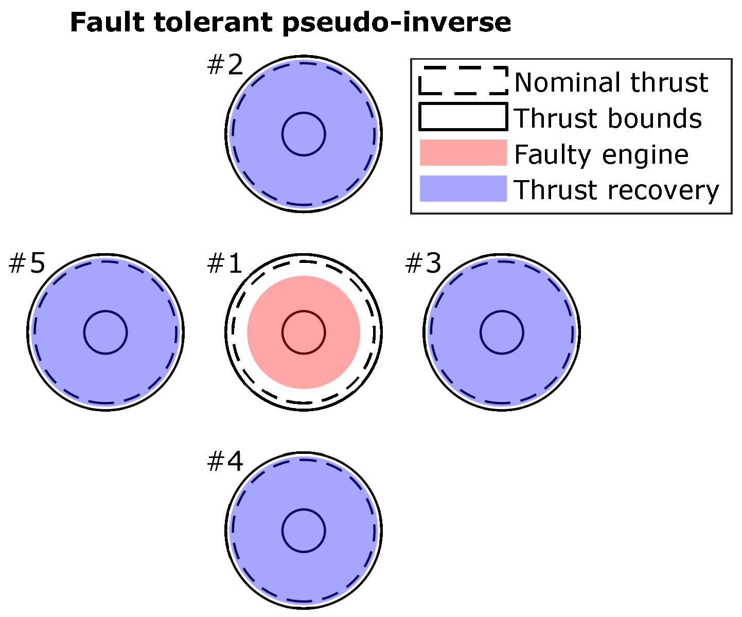
A key observation from Table 4 is that all dynamic allocation schemes exhibit similar behaviour, effectively achieving recovery with minimal residual and actuation norms. As illustrated in Figure 3, recovery is accomplished by increasing the thrust levels of the remaining healthy engines within the allowable re-throttling range. All recovery solutions distribute this additional thrust evenly among the healthy engines.

4.2. Non-Central Engine Failure

This failure scenario involves a 20% thrust loss in engine 2, one of the outer engines, as mathematically described in Equation (23). Similar to the central engine failure case, the fault in $T_2$ introduces a translational imbalance in the z-axis force equation. However, it also introduces additional effects, such as a reduction in the faulty engine’s effectiveness to generate moments (see red terms in matrix A) and the creation of parasitic moments in the y-axis (bottom red term in matrix C).

$$\left[\begin{array}{c}0\\ 0\\ 0\\ 0\\ 0\\ 5\end{array}\right]={\displaystyle \frac{\sqrt{2}}{2}}\left[\begin{array}{cccccccc}(0.8 · T_2)z_1& (0.8 · T_2)z_1& T_3{z}_1& T_3{z}_1& T_4{z}_1& T_4{z}_1& T_5{z}_1& T_5{z}_1\\ -(0.8 · T_2)z_1& (0.8 · T_2)z_1& -T_3{z}_1& T_3{z}_1& -T_4{z}_1& T_4{z}_1& -T_5{z}_1& T_5{z}_1\\ -(0.8 · T_2)x_2& -(0.8 · T_2)x_2& T_3{y}_3& -T_3{y}_3& T_4{x}_2& T_4{x}_2& -T_5{y}_3& T_5{y}_3\\ -(0.8 · T_2)& (0.8 · T_2)& -T_3& T_3& -T_4& T_4& -T_5& T_5\\ -(0.8 · T_2)& -(0.8 · T_2)& -T_3& -T_3& -T_4& -T_4& -T_5& -T_5\\ 0& 0& 0& 0& 0& 0& 0& 0\end{array}\right]\left[\begin{array}{c}{\delta }_{2,A}\\ {\delta }_{2,B}\\ {\delta }_{3,A}\\ {\delta }_{3,B}\\ {\delta }_{4,A}\\ {\delta }_{4,B}\\ {\delta }_{5,A}\\ {\delta }_{5,B}\end{array}\right]+\left[\begin{array}{c}{y}_3(T_3-T_5)\\ x_2(T_4-(0.8 · T_2))\\ 0\\ 0\\ 0\\ T_1+(0.8 · T_2)+T_3+T_4+T_5\end{array}\right]$$

(23)

The results are presented in

Table 5. Linear analysis results: non-central engine failure.

Variable	Fault-Tolerant Pseudo-Inv	Convex Opt.	Interior-Point Opt.	Pattern Search Opt.	Nonlinear Least Squares Opt.
${\parallel \mathbf{R}\parallel }_2$	15 $·$ ${10}^{-3}$	6 $·$ ${10}^{-3}$	6 $·$ ${10}^{-3}$	6 $·$ ${10}^{-3}$	6 $·$ ${10}^{-3}$
${\parallel \mathsf{\Gamma }\parallel }_2$	0.428	0.173	0.1725	0.1738	0.1729
$T_1$	1.05	1.1	1.1	1.0998	1.1
$T_2$	$0.8$	$0.8$	$0.8$	$0.8$	$0.8$
$T_3$	1.05	1.1	1.1	1.0998	1.1
$T_4$	1.05	0.9	0.9	0.9006	0.9
$T_5$	1.05	1.1	1.1	1.0998	1.1
${\delta }_{2,A}$ (m deg)	−121.9	−49.9	−49.6	−52	−49.7
${\delta }_{2,B}$ (m deg)	121.9	49.9	49.6	48	49.7
${\delta }_{3,A}$ (m deg)	−160	−68.3	−68.2	−70.3	−68.4
${\delta }_{3,B}$ (m deg))	160	68.3	68.2	71.4	68.4
${\delta }_{4,A}$ (m deg)	−160	−56.1	−55.8	−58.7	−55.9
${\delta }_{4,B}$ (m deg)	160	56.1	55.8	62.5	55.9
${\delta }_{5,A}$ (m deg)	−160	−68.3	−68.2	−63.2	−68.4
${\delta }_{5,B}$ (m deg)	160	68.3	68.2	61.8	68.4

, which also includes the allocated TVC actuator deflections for comparison. In this scenario, recovery is achieved by increasing the thrust levels of the healthy engines to restore the commanded z-axis force while deflecting the TVC actuators to counteract the parasitic moments caused by the thrust imbalance between engines 2 and 4.

The fault-tolerant pseudo-inverse recovery method distributes the additional thrust evenly among the healthy engines. However, this increases the thrust disparity between the axisymmetric engines 2 and 4, leading to a higher residual norm compared to the other approaches. This recovery solution is illustrated in Figure 4a, which also depicts the resulting body-frame forces generated by the dynamic allocation action.

In contrast, the other dynamic allocation functions prioritize minimizing the residual norm by reducing the thrust level of engine 4 as much as possible while still recovering the commanded total z-axis thrust level. All optimization-based schemes provide similar recovery actions in both thrust distribution and TVC deflections. This behavior is illustrated in Figure 4b for the convex recovery case. Interestingly, the resulting recovery forces align well in direction with those obtained using the fault-tolerant pseudo-inverse solution, as shown in Figure 4a.

4.3. TVC Jamming Failure

This failure scenario considers a 3° jamming failure in one of the TVC actuators of engine 3 (${\delta }_{3,A}$), as defined in Equation (24). This poses a significant challenge since the actuator is locked at half of its total TVC actuation range, as specified in Table 3.

$$\left[\begin{array}{c}0\\ 0\\ 0\\ 0\\ 0\\ T_c\end{array}\right]={\displaystyle \frac{\sqrt{2}}{2}}\left[\begin{array}{cccccccc}{T}_2{z}_1& T_2{z}_1& T_3{z}_1& T_3{z}_1& T_4{z}_1& T_4{z}_1& T_5{z}_1& T_5{z}_1\\ -T_2{z}_1& T_2{z}_1& -T_3{z}_1& T_3{z}_1& -T_4{z}_1& T_4{z}_1& -T_5{z}_1& T_5{z}_1\\ -T_2{x}_2& -T_2{x}_2& T_3{y}_3& -T_3{y}_3& T_4{x}_2& T_4{x}_2& -T_5{y}_3& T_5{y}_3\\ -T_2& T_2& -T_3& T_3& -T_4& T_4& -T_5& T_5\\ -T_2& -T_2& -T_3& -T_3& -T_4& -T_4& -T_5& -T_5\\ 0& 0& 0& 0& 0& 0& 0& 0\end{array}\right]\left[\begin{array}{c}{\delta }_{2,A}\\ {\delta }_{2,B}\\ 3{\displaystyle \frac{\pi }{180}}\\ {\delta }_{3,B}\\ {\delta }_{4,A}\\ {\delta }_{4,B}\\ {\delta }_{5,A}\\ {\delta }_{5,B}\end{array}\right]+\left[\begin{array}{c}{y}_3(T_3-T_5)\\ x_2(T_4-T_2)\\ 0\\ 0\\ 0\\ T_1+T_2+T_3+T_4+T_5\end{array}\right]$$

(24)

The results for this failure scenario are summarized in

Table 6. Linear analysis results: TVC jamming failure.

Variable	Fault-Tolerant Pseudo-Inv	Convex Opt.	Interior-Point Opt.	Pattern Search Opt.	Nonlinear Least Squares Opt.
${\parallel \mathbf{R}\parallel }_2$	6.3 $·$ ${10}^{-3}$	1.1 $·$ ${10}^{-4}$	3.49 $·$ ${10}^{-8}$	6.6 $·$ ${10}^{-5}$	4.9 $·$ ${10}^{-3}$
${\parallel \mathsf{\Gamma }\parallel }_2$	3.7947	3.7946	3.7826	3.8869	3.4583
$T_1$	1	1	1.0012	1	1.1
$T_2$	1	1	1.0051	1	1.1
$T_3$	1	1	0.9943	1	0.8503
$T_4$	1	1	1.0051	1	1.1
$T_5$	1	1	0.9943	1	0.8497
${\delta }_{2,A}$ (deg)	−0.6	−0.59	−0.59	−1.19	−0.58
${\delta }_{2,B}$ (deg)	0.6	0.58	0.59	0.59	0.39
${\delta }_{3,A}$ (deg)	3	3	3	3	3
${\delta }_{3,B}$ (deg)	0.6	0.62	0.59	0.59	0.31
${\delta }_{4,A}$ (deg)	−1.8	−1.79	−1.78	−1.8	−1.38
${\delta }_{4,B}$ (deg)	−0.6	−0.6	−0.59	−0.65	−0.39
${\delta }_{5,A}$ (deg)	−0.6	−0.6	−0.59	0	−0.45
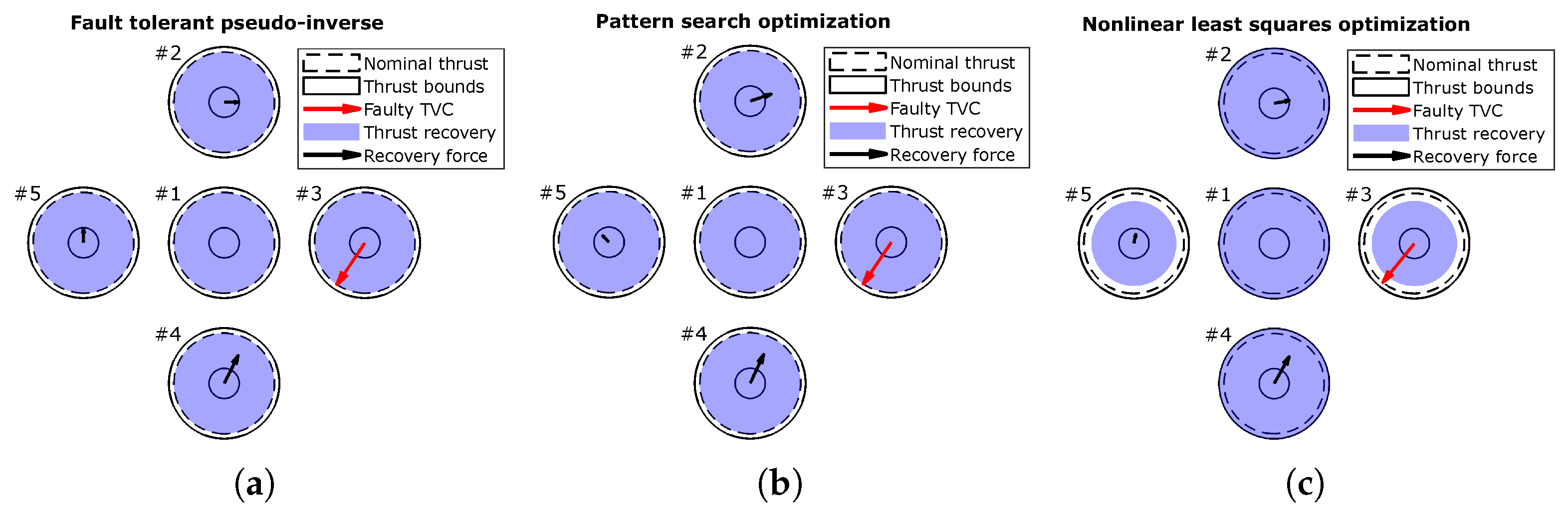
${\delta }_{5,B}$ (deg)	−0.6	−0.6	−0.59	−0.53	−0.3

. Notably, this problem does not have an unique solution, as all dynamic allocation approaches successfully achieve recovery with minimal residual norms, yet some of them differ in engine thrust distribution and, interestingly, in the direction of the resulting recovery forces.

The fault-tolerant pseudo-inverse, convex optimization and interior-point optimization recovery solutions exhibit very similar behavior. As exemplified in Figure 5a for the fault-tolerant pseudo-inverse case, these approaches mainly rely on TVC allocation while maintaining nominal engine throttling—or close to nominal in the case of the interior-point optimization approach.

The pattern search optimization method also relies solely on TVC allocation but results in a different direction for the recovery forces, as depicted in Figure 5b. In contrast, the nonlinear least squares optimization approach leads to a recovery action that combines both TVC deflections and adjustments to engine thrust levels, as shown in Figure 5c. Notably, this thrust reduction is applied to the engine whose actuator is faulty, and to the asymmetric engine 5 to avoid additional parasitic forces and moments.

4.4. Simultaneous Engine and TVC Failure

The last failure scenario involves two simultaneous faults: a 20% thrust loss in engine 3 and a 3° jamming failure in one of the TVC actuators of engine 4 (${\delta }_{4,b}$), as mathematically defined in Equation (25).

$$\left[\begin{array}{c}0\\ 0\\ 0\\ 0\\ 0\\ T_c\end{array}\right]={\displaystyle \frac{\sqrt{2}}{2}}\left[\begin{array}{cccccccc}{T}_2{z}_1& T_2{z}_1& (0.8 · T_3)z_1& (0.8 · T_3)z_1& T_4{z}_1& T_4{z}_1& T_5{z}_1& T_5{z}_1\\ -T_2{z}_1& T_2{z}_1& -(0.8 · T_3)z_1& (0.8 · T_3)z_1& -T_4{z}_1& T_4{z}_1& -T_5{z}_1& T_5{z}_1\\ -T_2{x}_2& -T_2{x}_2& (0.8 · T_3)y_3& -(0.8 · T_3)y_3& T_4{x}_2& T_4{x}_2& -T_5{y}_3& T_5{y}_3\\ -T_2& T_2& -(0.8 · T_3)& (0.8 · T_3)& -T_4& T_4& -T_5& T_5\\ -T_2& -T_2& -(0.8 · T_3)& -(0.8 · T_3)& -T_4& -T_4& -T_5& -T_5\\ 0& 0& 0& 0& 0& 0& 0& 0\end{array}\right]\left[\begin{array}{c}{\delta }_{2,A}\\ {\delta }_{2,B}\\ {\delta }_{3,A}\\ {\delta }_{3,B}\\ {\delta }_{4,A}\\ 3{\displaystyle \frac{\pi }{180}}\\ {\delta }_{5,A}\\ {\delta }_{5,B}\end{array}\right]+\left[\begin{array}{c}{y}_3((0.8 · T_3)-T_5)\\ x_2(T_4-T_2)\\ 0\\ 0\\ 0\\ T_1+T_2+(0.8 · T_3)+T_4+T_5\end{array}\right]$$

(25)

The results for this failure scenario, presented in

Table 7. Linear analysis results: simultaneous non-central engine and TVC jamming failure.

Variable	Fault-Tolerant Pseudo-Inv	Convex Opt.	Interior Point Opt.	Pattern Search Opt.	Nonlinear Least Squares Opt.
${\parallel \mathbf{R}\parallel }_2$	15 $·$ ${10}^{-3}$	6 $·$ ${10}^{-3}$	6.4 $·$ ${10}^{-3}$	8.4 $·$ ${10}^{-3}$	10 $·$ ${10}^{-3}$
${\parallel \mathsf{\Gamma }\parallel }_2$	4.0675	4.1627	4.1093	4.1585	3.9813
$T_1$	1.05	1.1	1.1	1.0998	1.1
$T_2$	1.05	1.1	1.1	1.0998	1.1
$T_3$	$0.8$	$0.8$	$0.8$	$0.8$	$0.8$
$T_4$	1.05	1.1	1.1	1.0998	1.1
$T_5$	1.05	0.9	0.9	0.9006	0.9
${\delta }_{2,A}$ (deg)	0.41	0.74	0.68	0.85	0.55
${\delta }_{2,B}$ (deg)	−0.88	−0.94	−0.98	−1.43	−1.06
${\delta }_{3,A}$ (deg)	−0.67	−0.71	−0.65	−1.19	−0.54
${\delta }_{3,B}$ (deg)	−0.67	−0.69	−0.71	−0.26	−0.77
${\delta }_{4,A}$ (deg)	−0.88	−0.93	−0.89	−0.39	−0.74
${\delta }_{4,B}$ (deg)	3	3	3	3	3
${\delta }_{5,A}$ (deg)	0.41	0.6	0.56	0.22	0.45
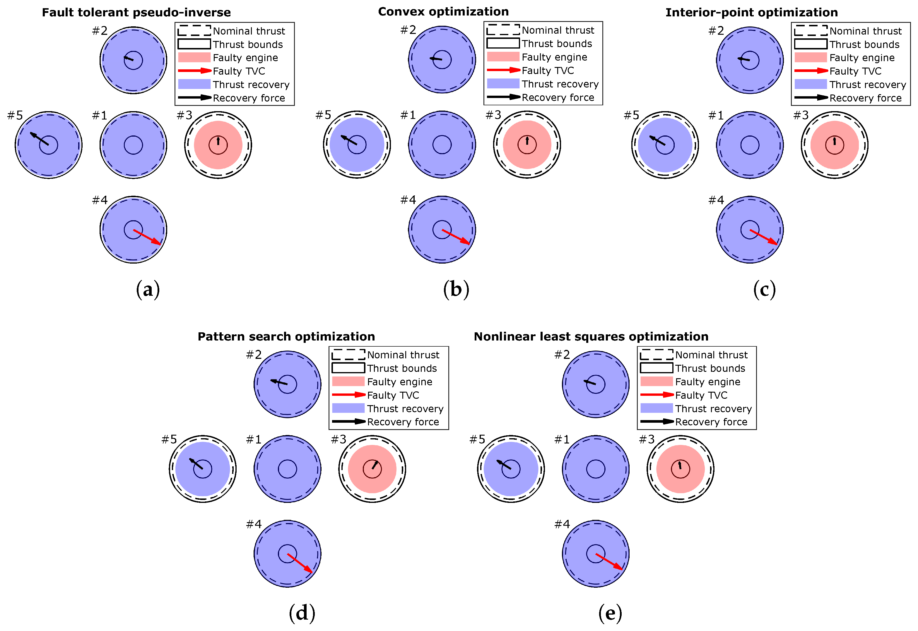
${\delta }_{5,B}$ (deg)	−2.17	−2.15	−2.09	−1.95	−1.93

and Figure 6, demonstrate the ability of dynamic allocation functions to handle simultaneous failures in axis-asymmetric engines. In all cases, recovery is achieved through a combination of TVC re-allocation and engine thrust adjustments.

As observed in Section 4.2, the fault-tolerant pseudo-inverse solution distributes the additional thrust evenly among the healthy engines. While this strategy ensures recovery, it results in higher residual and actuation norms compared to the other methods.

In contrast, the optimization-based approaches minimize the residual norm by strategically reducing the thrust level of the asymmetric engine 5, ensuring that the commanded total z-axis thrust level is maintained. Interestingly, they differ in the recovery TVC deflections, leading to slight variations in the resulting recovery forces as illustrated in Figure 6.

5. Nonlinear Comparison

This section evaluates and compares a selection of the dynamic allocation recovery strategies from Section 3 using the nonlinear simulator described in Section 2.3. In particular, the fault-tolerant pseudo-inverse, convex optimization, and constrained optimization (interior-point approach via fmincon) allocation schemes are assessed across four distinct failure scenarios: (1) 20% loss of thrust in the central engine (Section 5.1); (2) 20% loss of thrust in outer engine 2 (Section 5.2); (3) TVC jamming (Section 5.3); and (4) simultaneous engine and TVC failure (Section 5.4).

It is important to note that the optimization weights were adjusted, as indicated in

Table 8. Optimization weights used in the nonlinear analysis.

Optimization Approach	Parameter	Value
Convex opt.	Optimization weight ${\lambda }_1$ (residual)	1
	Optimization weight ${\lambda }_2$ (throttling actuation)	1
Interior-point opt.	Optimization weight ${\lambda }_1$ (residual)	20
	Optimization weight ${\lambda }_2$ (throttling actuation)	10
	Optimization weight ${\lambda }_3$ (TVC actuation)	0.1

, to ensure the proper functioning of the dynamic allocation across all considered failures within the nonlinear simulator setup. In particular, the throttling actuation weight was increased in both cases to prevent recurrent re-throttling among the engines, ensuring a more stable and efficient recovery response.

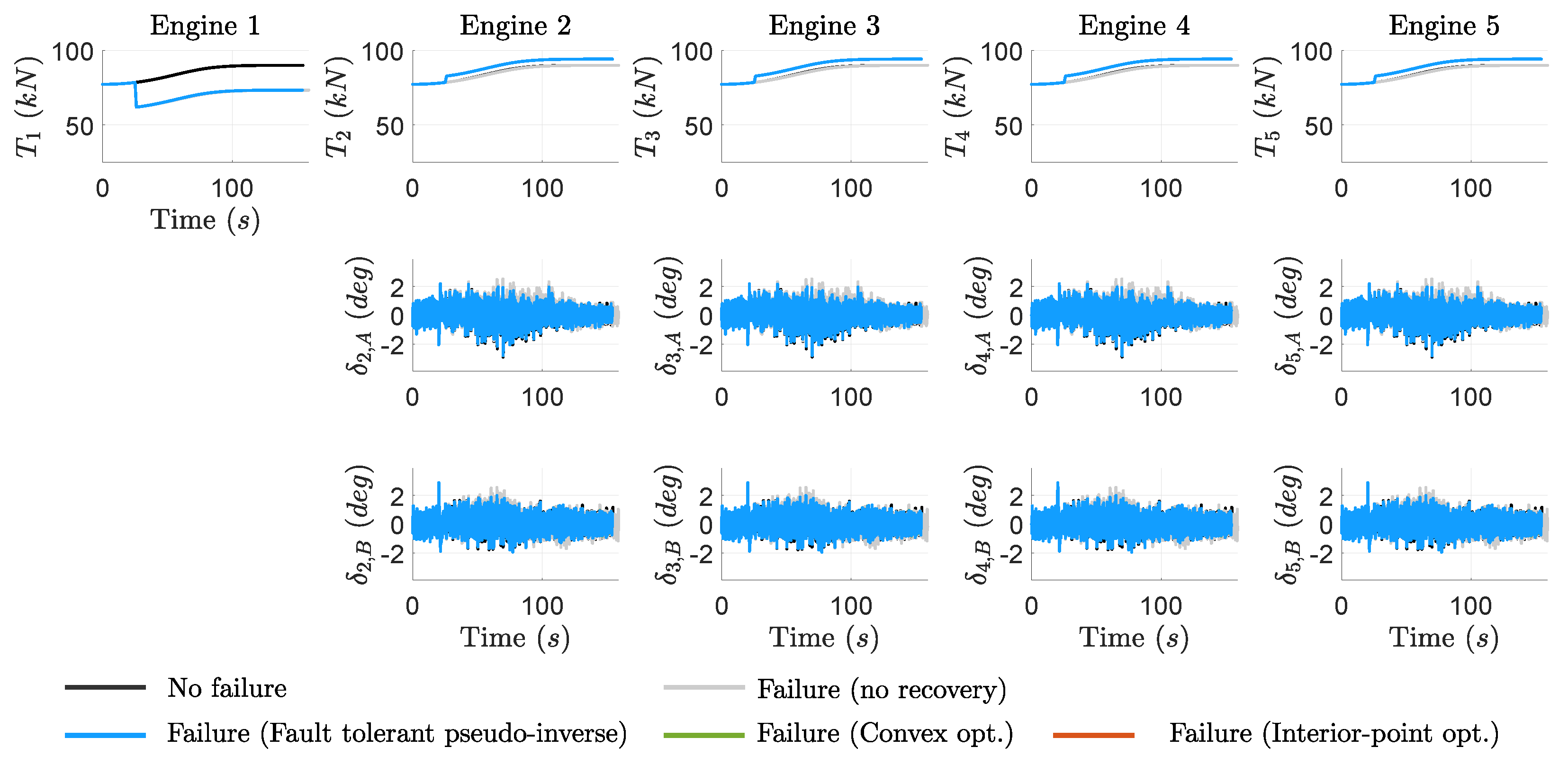
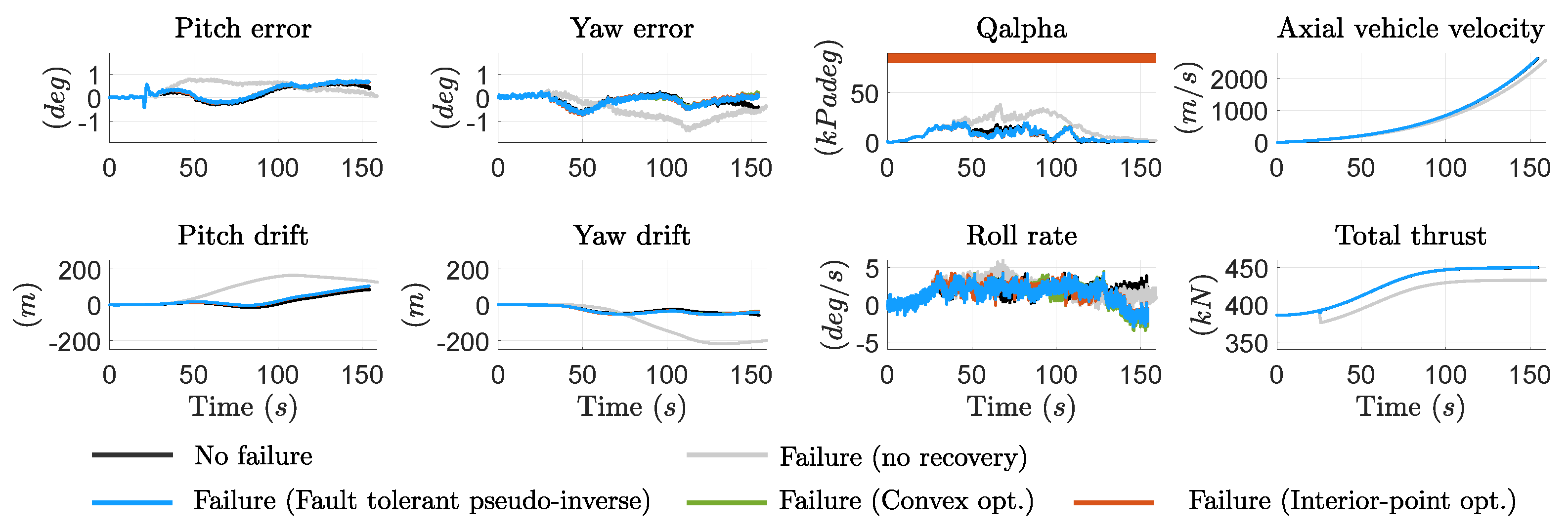
5.1. Central Engine Failure

The first failure test consists of a 20% thrust loss in the central engine, triggered at $t=$ 25 $\mathrm{s}$. Figure 7 illustrates the time-domain performance of key launch vehicle indicators during ascent, while Figure 8 displays the overall actuation response, including engine thrust levels and TVC deflections. As aforementioned, three recovery strategies are compared: fault-tolerant pseudo-inverse (green solid lines), convex-based optimization (blue solid lines), and interior-point optimization (orange solid lines). It is noted that the baseline (no failure) case (black solid lines) and the failure case without recovery action (gray solid lines) are also included to serve as references.

Figure 7 highlights the significant degradation in system performance when no recovery action is taken (see gray lines). The propulsion failure in the central engine results in large deviations in critical metrics such as attitude error, lateral drift, and $Q\alpha$, as well as extended first stage duration.

All tested dynamic allocation recovery strategies effectively restore system performance to levels comparable to the baseline non-faulty case. The resulting recovery responses are superposed in the figures as they provide approximately the same system responses, with only minor variations observed in the roll-rate profile. In all cases, the recovery is achieved by increasing the thrust levels of the remaining healthy engines to compensate for the lost thrust, as shown in the upper plots of Figure 8.

A key factor in evaluating the recovery solutions is the level of TVC actuation required.

Table 9. Nonlinear analysis results: TVC integrated angle analysis.

Failure Case	Total Integrated Angle (deg)
	No Failure	No Recovery	Pseudo-Inverse	Convex	Interior-Point
Central engine	558.15	610.68	538.14	538.26	537.78
Non-central engine	558.15	603.53	568.15	568.23	567.36
TVC jamming	558.15	2181.2	761	761.03	760.9
Engine + TVC	558.15	2772.5	845.4	846.68	845.37

presents the total integrated angle for each failure case and recovery method. Among the tested strategies, the interior-point optimization solution exhibits the lowest actuation effort, though the difference compared to the other approaches is minimal.

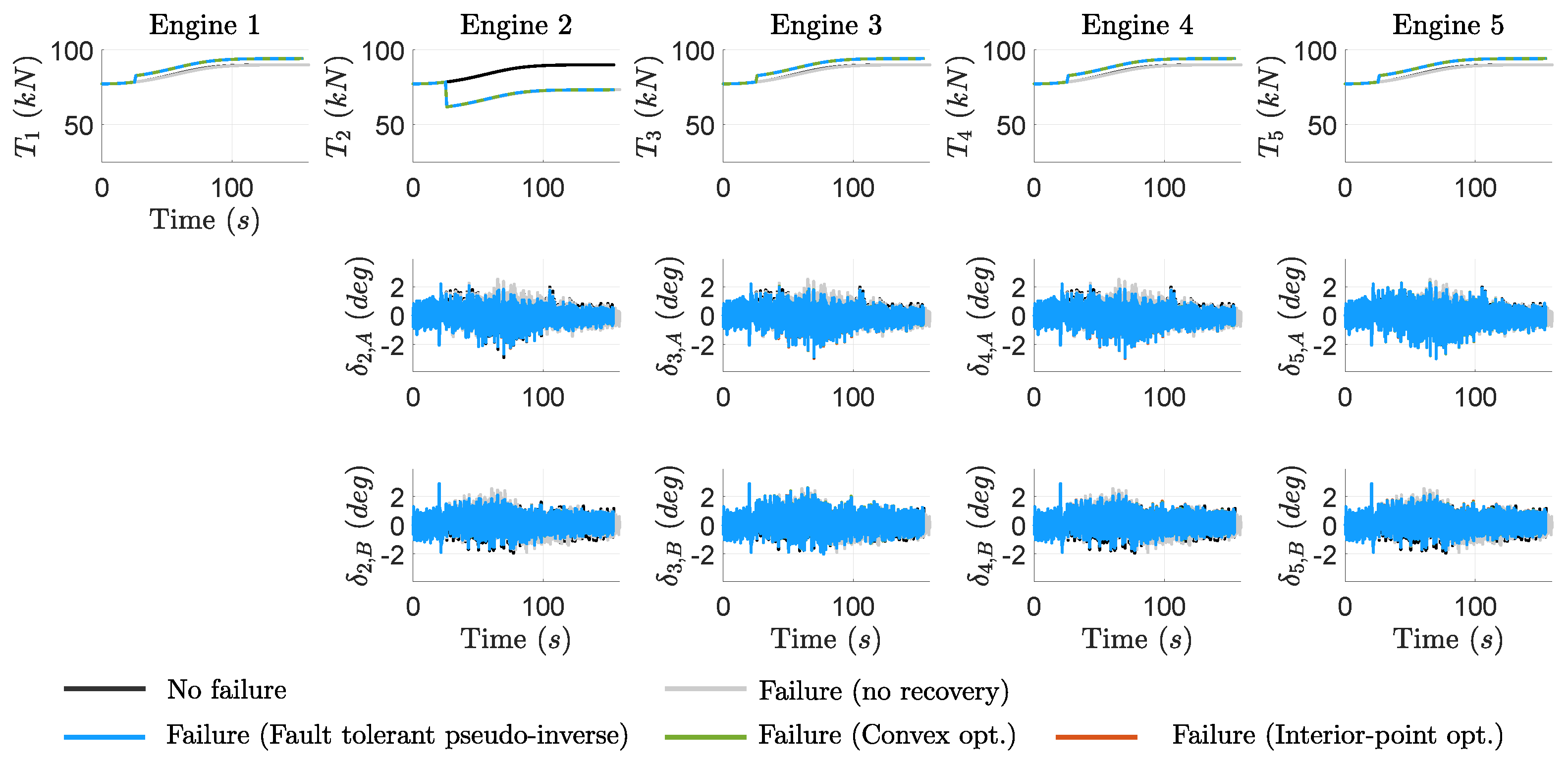
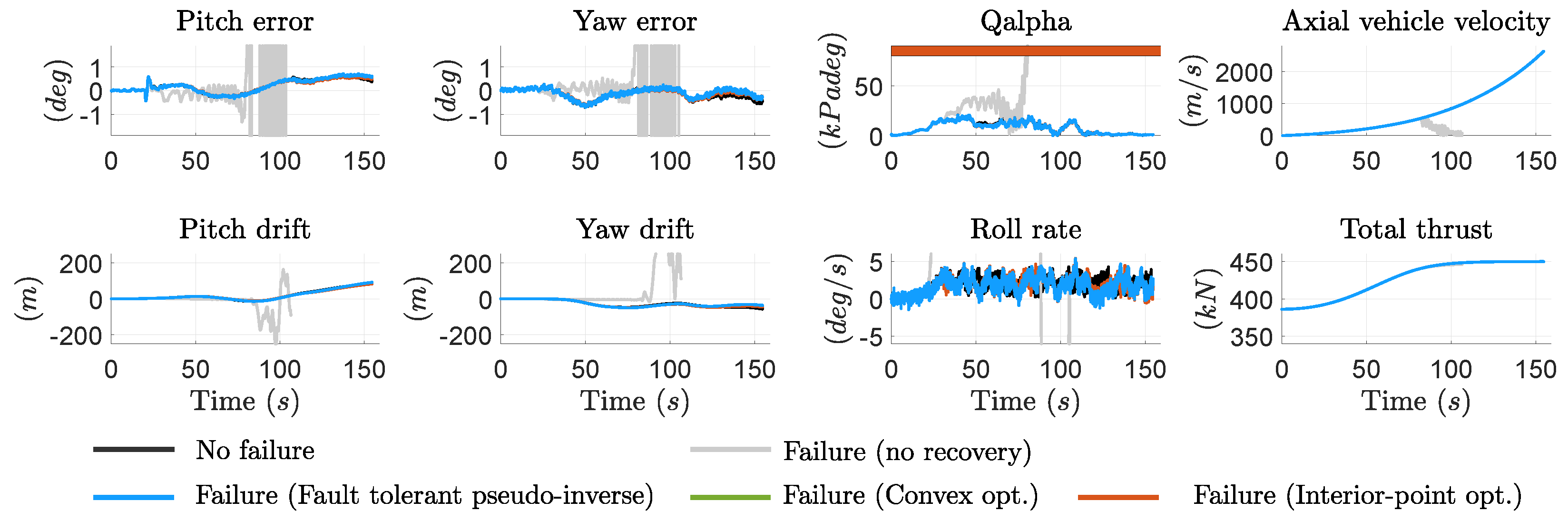
5.2. Non-Central Engine Failure

The second failure scenario involves a 20% thrust loss in outer engine 2, triggered at $t=$ 25 $\mathrm{s}$. Similarly to the central engine failure case, the absence of a recovery action results in significant performance degradation and an extended first stage duration.

Figure 9 shows that all the recovery solutions effectively restore key trajectory parameters, as shown in the axial vehicle velocity and total thrust plots. The recovery is also achieved by increasing the non-faulty engines, as illustrated in the upper plots of Figure 10. However, they present some deviations in attitude, drift, and $Q\alpha$ when compared to the baseline non-faulty case. These discrepancies can be attributed to two main factors: (1) the failure induces parasitic forces and torques along the pitch axis due to the asymmetric thrust distribution between engines 2 and 4, which cannot be compensated by the dynamic allocation functions; and (2) variations in the roll dynamics, as seen in the roll rate plot in Figure 10, also may contribute to the observed differences.

As in the previous failure case, the recovery responses are nearly identical with only minor differences in attitude error and more noticeable variations in the roll rate profile. In addition, the same trend in TVC allocation effort is observed in Table 9, where the interior-point optimization approach requires the least TVC actuation effort.

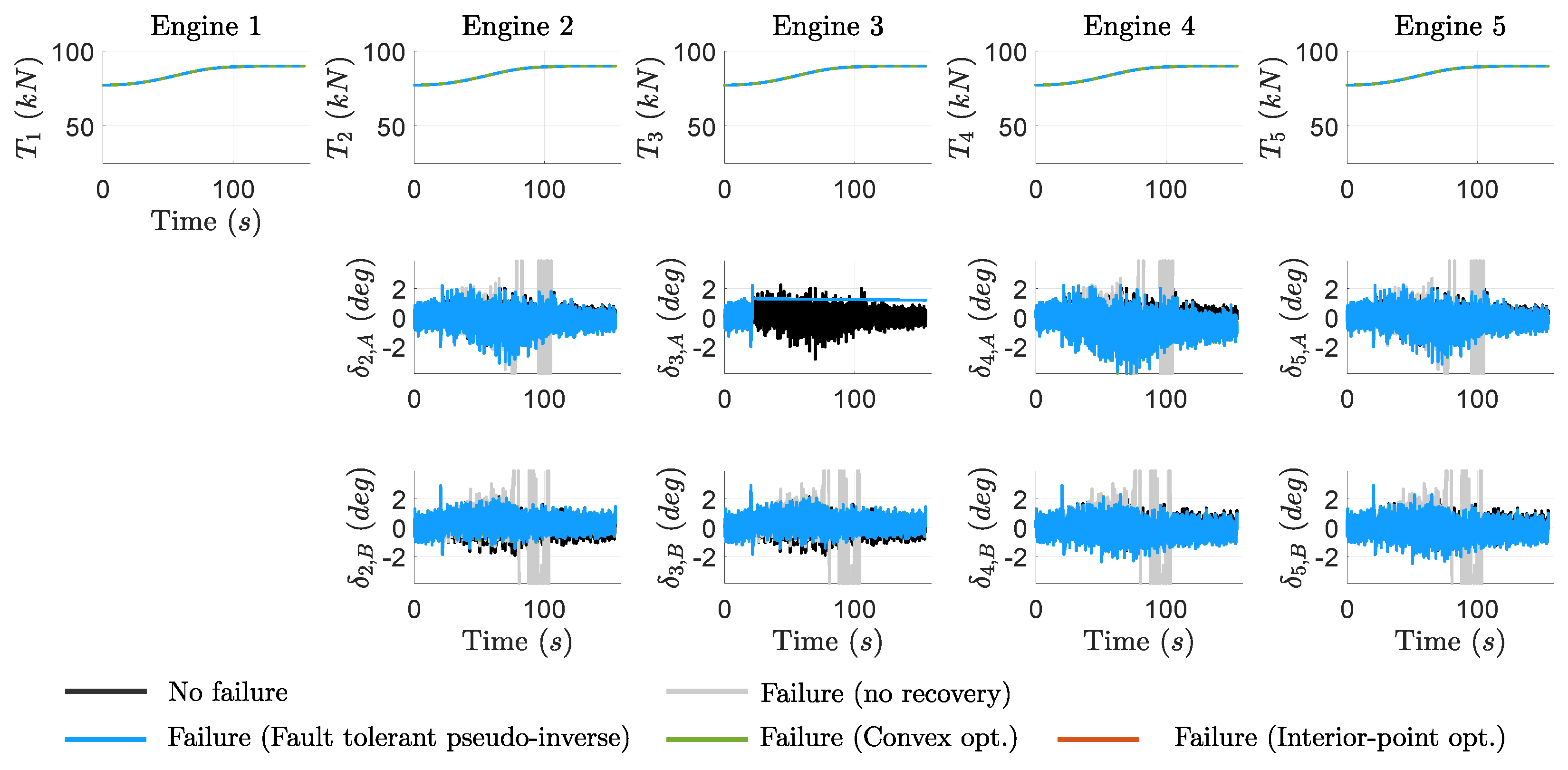
5.3. TVC Jamming Failure

The third failure scenario involves a TVC jamming failure occurring at $t=$ $21.4$ $\mathrm{s}$ in the first TVC actuator of engine 3, see results in Figure 11 and Figure 12. This failure causes the actuator to remain locked at a constant deflection of 1.2°, as shown in Figure 12 (see ${\delta }_{3,A}$ plot).

Figure 11 illustrates that, without a recovery action (see gray lines), the TVC jamming failure causes the loss of the vehicle. In particular, this results in unacceptable attitude and drift-rate oscillations as well as a violation of the $Q\alpha$ requirement. In contrast, all the dynamic allocation schemes prevent the loss of the vehicle, restoring key trajectory parameters to closely match the baseline non-faulty case, as observed in the axial vehicle velocity, $Q\alpha$, and total thrust plots in Figure 11.

The recovery is achieved by re-allocating the remaining healthy TVC actuators to counteract the forces and moments induced by the jammed actuator. As a result, the total integrated TVC angle for this failure case is significantly higher than in the two previous fault scenarios, as shown in Table 9.

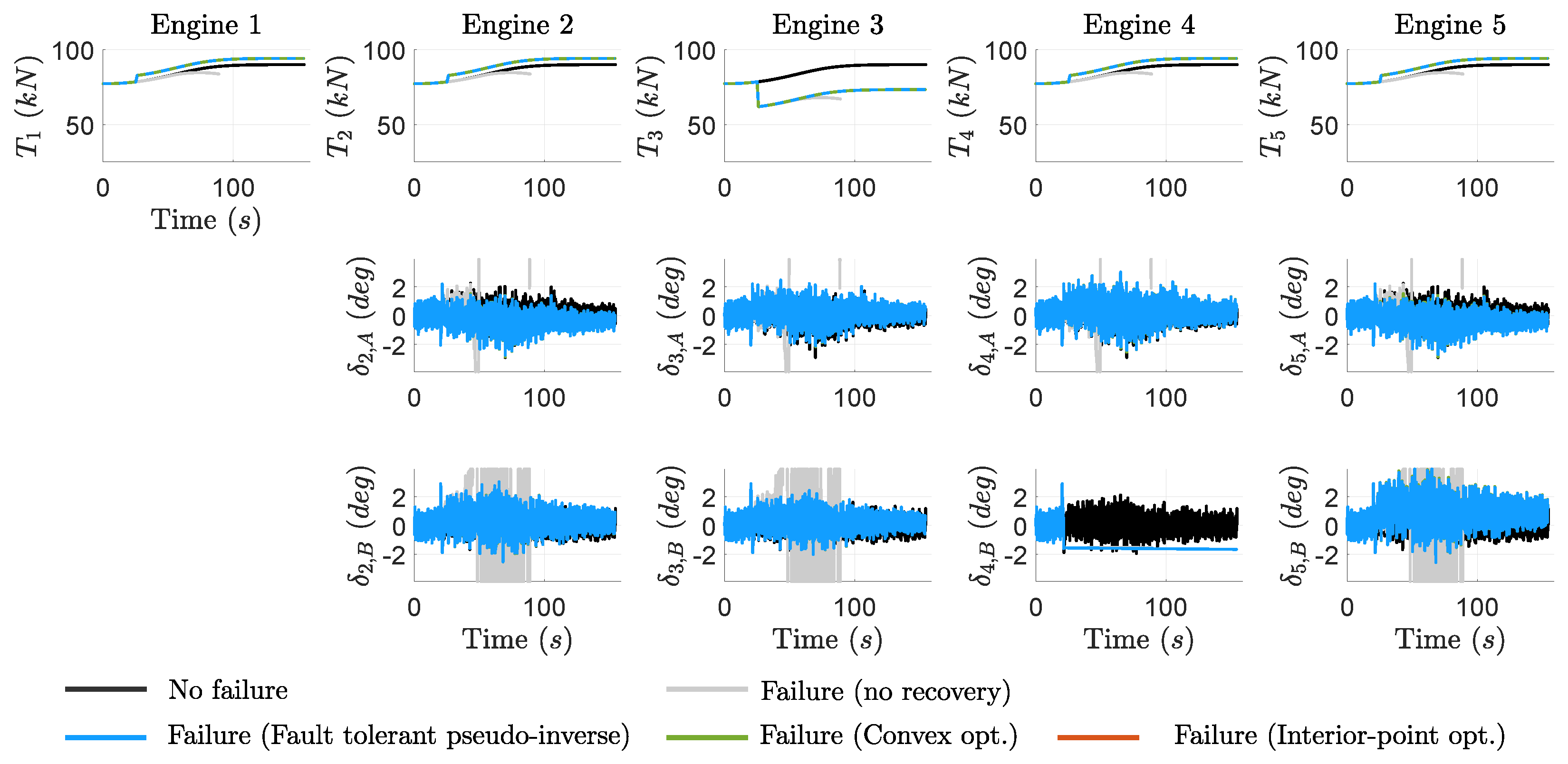
5.4. Simultaneous Engine and TVC Failure

The last failure scenario consists of a simultaneous TVC jamming failure and a 20% thrust loss in an outer engine, see results in Figure 13 and Figure 14. The TVC jamming occurs at $t=$ $21.4$ $\mathrm{s}$ in the second TVC actuator of engine 4, resulting in a constant deflection of −1.64°, as shown in the ${\delta }_{4,B}$ plot of Figure 14. Additionally, at $t=$ 25 $\mathrm{s}$, engine 3 experiences a 20% thrust loss, further challenging the system’s ability to maintain stability and performance.

Similar to the TVC jamming case, the absence of a recovery action results in a loss of the vehicle due to the destabilizing effects of the failures. However, the dynamic allocation strategies effectively compensate both faults, successfully restoring the vehicle’s responses to closely match that of the baseline non-faulty case. Furthermore, this simultaneous failure scenario demands an even higher level of TVC actuation for successful recovery compared to the previous three fault cases, as indicated in Table 9.

6. Conclusions

This article presents and evaluates various fault-tolerant dynamic allocation strategies designed to mitigate propulsion and actuation failures in launch vehicles using a clustered engine configuration. The results demonstrate that these strategies can successfully recover up to 40% propulsion loss in a single engine, considering the given cluster configuration and the 110% re-throttling constraint of the employed engines. Furthermore, the strategies can cope with actuator failures, such as TVC jamming, and simultaneous propulsion and actuation failures.

Among the dynamic allocation methods examined, optimization-based solutions provide optimal performance. However, careful attention must be given to defining the cost function and assigning appropriate weights to effectively balance multiple objectives, such as minimizing moment and force residuals, reducing actuation efforts, and ensuring a feasible engine throttling profile. Additionally, real-time implementation of these optimization-based approaches poses challenges due to the high sampling rate of the on-board computer, potential high computational load, and possible convergence issues.

In contrast, the fault-tolerant pseudo-inverse approach, while not optimal, provides recovery solutions that closely match those of the optimization-based methods. Its straightforward implementation and low computational cost make it a strong candidate for on-board deployment, offering a practical and efficient alternative for real-time failure recovery.

Future work could focus on evaluating the robustness of the proposed strategies under more complex failure combinations and across different phases of flight, as well as assessing their real-time performance and implementation feasibility.

References

- Song, Z.; Pan, H.; Zhao, Y.; Yao, W.; He, Y.; Wang, C. Reviews and Challenges in Reliability Design of Long March Launcher Control Systems. AIAA J. 2022, 60, 537–550. [Google Scholar] [CrossRef]
- Goupil, P.; Marcos, A. The European ADDSAFE project: Industrial and academic efforts towards advanced fault diagnosis. Control Eng. Pract. 2014, 31, 109–125. [Google Scholar] [CrossRef]
- Goupil, P.; Boada-Bauxell, J.; Marcos, A.; Rosa, P.; Kerr, M.; Dalbies, L. An overview of the FP7 RECONFIGURE project: Industrial, scientific and technological objectives. IFAC-PapersOnLine 2015, 48, 976–981. [Google Scholar] [CrossRef]
- Marcos, A.; Waitman, S.; Sato, M. Fault tolerant linear parameter varying flight control design, verification and validation. J. Frankl. Inst. 2022, 359, 653–676. [Google Scholar] [CrossRef]
- Marcos, A.; Peñín, L.; Gonidec, S.L.; Lemaitre, A. HMS-Control-Interaction architecture for rocket engines. In Proceedings of the AIAA Guidance, Navigation, and Control Conference, Minneapolis, MN, USA, 13–16 August 2012. [Google Scholar] [CrossRef]
- Marcos, A.; Peñín, L.; Malikov, D.; Reichstadt, S.; Gonidec, S.L. Fault Detection and Isolation for a Rocket Engine Valve. IFAC Proc. Vol. 2013, 46, 101–106. [Google Scholar] [CrossRef]
- Murata, R.; Thioulouse, L.; Marzat, J.; Piet-Lahanier, H.; Galeotta, M.; Farago, F. Optimal reconfigurable allocation of a multi-engine cluster for a reusable launch vehicle. In Proceedings of the 9th European Conference for Aerospace Sciences, Lille, France, 27 June–1 July 2022. [Google Scholar]
- Fari, S.; Seelbinder, D.; Theil, S.; Simplício, P. Robust Fault Detection and Isolation algorithms for TVC systems: An experimental test. In Proceedings of the 75th International Astronautical Congress, Milan, Italy, 14–18 October 2024. IAC-24-D2-6-9-x87783. [Google Scholar]
- Navarro-Tapia, D.; Simplício, P.; Marcos, A. Fault Tolerant Control Synthesis for a Cluster of Rocket Engines. In Proceedings of the 11th IFAC Symposium on Robust Control Design (ROCOND), Porto, Portugal, 2–4 July 2025. [Google Scholar]
- Paulino, N.; Roche Arroyos, C.; Ferreira, L.; Pascucci, M.; Arnedo García, J.; Navarro-Tapia, D.; Marcos, A.; Lalami, M.; Alexandre, P.; Simplício, P.; et al. Fault Tolerant Control for a Cluster of Rocket Engines—Methods and outcomes for guidance and control recovery strategies in launchers. In Proceedings of the ESA 12th International Conference on Guidance Navigation and Control and 9th International Conference on Astrodynamics Tools and Technique, ESA, Sopot, Poland, 12–16 June 2023. [Google Scholar] [CrossRef]
- Roche Arroyos, C.; Pascucci, M.; Paulino, N.; Arnedo, J.; Navarro-Tapia, D.; Marcos, A.; Lalami, M.; Alexandre, P.; Simplício, P.; Casasco, M. Fault-Tolerant Control for a Cluster of Rocket Engines—Results for launch and landing of a re-usable launcher. In Proceedings of the 2024 CEAS EuroGNC Conference, CEAS EuroGNC, Bristol, UK, 11–13 June 2024. CEAS-GNC-2024-045. [Google Scholar]
- Orr, J.S.; Slegers, N.J. High-Efficiency Thrust Vector Control Allocation. J. Guid. Control. Dyn. 2014, 37, 374–382. [Google Scholar] [CrossRef]
- Navarro-Tapia, D.; Marcos, A.; Simplício, P.; Bennani, S.; Roux, C. Legacy recovery and robust augmentation structured design for the VEGA launcher. Int. J. Robust Nonlinear Control. 2019, 29, 3363–3388. [Google Scholar] [CrossRef]
- Navarro-Tapia, D. Robust and Adaptive TVC Control Design Approaches for the VEGA Launcher. Ph.D. Thesis, University of Bristol, Bristol, UK, 2019. [Google Scholar]
- Doyle, J.C.; Packard, A.; Zhou, K. Review of LFTs, LMIs, and μ. In Proceedings of the 30th IEEE Conference on Decision and Control, Brighton, UK, 11–13 December 1991; pp. 1227–1232. [Google Scholar]
- Marcos, A.; Mostaza, D.; Peñín, L.F. Achievable Moments NDI-based Fault Tolerant Thrust Vector Control of an Atmospheric Vehicle during Ascent. IFAC Proc. Vol. 2009, 42, 621–626. [Google Scholar] [CrossRef]
- Pascucci, C.A.; Szmuk, M.; Açikmeşe, B. Optimal control allocation for a multi-engine overactuated spacecraft. In Proceedings of the 2017 IEEE Aerospace Conference, Big Sky, MT, USA, 4–11 March 2017; pp. 1–6. [Google Scholar] [CrossRef]
- Grant, M.; Boyd, S. Graph implementations for nonsmooth convex programs. In Recent Advances in Learning and Control; Blondel, V., Boyd, S., Kimura, H., Eds.; Lecture Notes in Control and Information Sciences; Springer: Berlin/Heidelberg, Germany, 2008; pp. 95–110. [Google Scholar]
- CVX Research, Inc. CVX: Matlab Software for Disciplined Convex Programming, Version 2.0. 2012. Available online: https://cvxr.com (accessed on 29 April 2025).
- Mattingley, J.; Boyd, S. CVXGEN: A code generator for embedded convex optimization. Optim. Eng. 2012, 13, 1–27. [Google Scholar] [CrossRef]
- Diamond, S.; Boyd, S. CVXPY: A Python-Embedded Modeling Language for Convex Optimization. J. Mach. Learn. Res. 2016, 17, 1–5. [Google Scholar]
- MATLAB. Optimization Toolbox; The MathWorks: Natick, MA, USA, 2023. [Google Scholar]
- MATLAB. Global Optimization Toolbox; The MathWorks: Natick, MA, USA, 2023. [Google Scholar]
Figure 1.
Cluster of engines’ configuration.
Figure 2.
Simplified block diagram of the FES for a dynamic allocation reconfiguration case (nominal GNC in black; FDIR GNC functionalities in blue).
Figure 3.
Fault-tolerant pseudo-inverse recovery solution for a central engine failure.
Figure 4.
Recovery solutions for a non-central engine failure: (a) fault-tolerant pseudo-inverse solution; (b) convex optimization solution.
Figure 5.
Recovery solutions for a TVC jamming failure: (a) fault-tolerant pseudo-inverse solution; (b) pattern search optimization solution; (c) nonlinear least squares optimization solution.
Figure 6.
Recovery solutions for a simultaneous non-central engine and TVC jamming failure: (a) fault-tolerant pseudo-inverse solution; (b) convex optimization solution; (c) interior-point optimization solution; (d) pattern search solution; (e) nonlinear least squares optimization solution.
Figure 7.
Central engine failure: key variables.
Figure 8.
Central engine failure: actuation.
Figure 9.
Non-central engine failure: time-domain nonlinear key variables.
Figure 10.
Non-central engine failure: actuation.
Figure 11.
TVC jamming failure: time-domain nonlinear key variables.
Figure 12.
TVC jamming failure: actuation.
Figure 13.
Simultaneous engine and TVC failure: time-domain nonlinear key variables.
Figure 14.
Simultaneous engine and TVC failure: actuation.