Article

Electromechanical Resonant Ice Protection Systems Using Extensional Modes: Optimization of Composite Structures

by
Giulia Gastaldo
1,*,
Younes Rafik
2,
Marc Budinger
2,* and
Valérie Pommier-Budinger
1
1
Fédération ENAC ISAE-SUPAERO ONERA, University of Toulouse, 31400 Toulouse, France
2
Institut Clement Ader, University of Toulouse, INSA, ISAE-SUPAERO, MINES ALBI, UPS, CNRS, 31055 Toulouse, France
*
Authors to whom correspondence should be addressed.
Aerospace 2025, 12(3), 255; https://doi.org/10.3390/aerospace12030255
Submission received: 24 February 2025 / Revised: 13 March 2025 / Accepted: 14 March 2025 / Published: 18 March 2025
(This article belongs to the Section Aeronautics)

Abstract

:
Efficient ice protection systems are essential to ensure the operability and reliability of aircraft. In recent years, electromechanical resonant ice protection systems have emerged as a promising low-power alternative to current solutions. These systems can operate in two primary resonant modes: flexural and extensional. While extensional modes enable effective de-icing over large surface areas, their performance can be compromised by interference from flexural modes, particularly in thin, ice-covered substrates where natural mode coupling occurs. This study presents a strategy based on material selection for making the Young’s modulus-to-density ratio uniform. The final objective of this paper is to establish the design rules for a composite leading edge de-icing system. For this purpose, an incremental approach will be used on profiles with different radii of curvature: plate or beam (infinite radius), circular profile (constant radius), NACA profile (variable radius). For beam and plate structures, the paper shows that this coupling can be mitigated by selecting materials with a Young’s modulus-to-density ratio comparable to that of ice. For curved structures, the curvature-induced effect is another source of parasitic flexion, which cannot be controlled solely by material selection and requires careful thickness optimization. This study presents analytical and numerical approaches to investigate the origin of this effect and a design methodology to minimize parasitic flexion in curved structures. The methodology is applied to the design optimization of a glass fiber NACA 0024 airfoil leading edge, the performance of which is subsequently evaluated through icing wind tunnel testing.

1. Introduction

Atmospheric icing represents a threat to aviation [1,2]. During flight, the supercooled water droplets suspended in the clouds impact the surfaces of the aircraft and freeze. This phenomenon alters the airfoil geometry, degrading the aerodynamic properties of the wing [3,4]. Furthermore, ice formation on air intake protection grids contributes to higher fuel consumption and power losses [5]. To overcome performance degradation and safety threats, the use of ice protection systems is necessary.
Thermal systems are the most common ice protection solutions for large jet aircraft, using hot bleed air from compressor stages [6]. These systems consume a significant amount of power. Moreover, considering the shift toward electric aircraft, they might not be a feasible solution in the future. Currently, the Boeing 787 is the only airliner equipped with an electrothermal de-icing system [7,8], using thermoelectric heating mats to protect the surfaces. However, this technology is also power-consuming, although recent research has focused on optimizing heat flux distribution to enhance the efficiency of electrothermal ice protection systems, significantly reducing power consumption [9]. Recently, electrothermal systems have also been studied for integration with glass fiber substrates [10].
Mechanical de-icing systems are less energy-consuming solutions, removing the ice layer by inducing fractures within the ice. Among these solutions, pneumatic systems are the ones used in regional jets and smaller aircraft. The main drawbacks of these systems are that they influence the overall aerodynamics of the aircraft and require regular maintenance due to the low material durability [11].
Recent studies highlight electromechanical resonant systems as a promising low-power alternative for ice protection. Palanque et al. [12] compared various systems on an Airbus A320, finding that electromechanical de-icing consumes 1.5–2 kW/m2, significantly less than evaporative thermal anti-icing (26.5 kW/m2), evaporative electrothermal anti-icing (20 kW/m2), and electrothermal de-icing (4 kW/m2).
Electromechanical de-icing systems use piezoelectric actuators to vibrate iced surfaces at one of their natural frequencies. This generates high stresses in the ice and facilitates the release of energy, causing the ice to fracture and detach from the surface [13,14,15,16,17,18,19].
The literature already contains a number of studies on electromechanical ice protection systems using composite materials. In a study conducted by Wang et al. [20], a carbon fiber reinforced plate was tested at a frequency of 34.8 kHz, and the ice was shed off the plate in approximately 3 min. It is assumed that the de-icing process is due to both mechanical and thermal effects arising from the extended excitation time. Zhu et al. [21] evaluated the performances of ultrasonic de-icing on a glass-fiber composite plate. The de-icing process lasted about 1 min and 28 s using a 38 kHz frequency and also resulted in a combination of thermal melting and delamination. To the best of the authors’ knowledge, no de-icing tests have been performed on composite structures to investigate ice-shedding behavior due to purely mechanical effects.
In this study, extensional modes are selected for an electromechanical resonant de-icing system designed for application on a composite substrate. Characterized by predominant in-plane motion, these modes facilitate efficient de-icing over large surface areas, provided they remain pure and do not interfere with out-of-plane flexural modes, which can degrade their performance [22,23].
However, as shown in [24], in a multi-material system such as an iced structure, obtaining a pure extensional mode can be challenging. The authors demonstrated the presence of some inertial coupling in the wave equations of a flat beam due to the presence of heterogeneous material properties along the thickness. This coupling leads to the presence of parasitic flexion in the extensional mode, which results in a less effective de-icing. It was shown that the inertial coupling is equal to zero if the Young’s modulus-to-density ratio ( E ρ ) is uniform throughout the structure. To this end, architectural materials were proposed as a potential solution to minimize the parasitic flexural ratio (PFR), aiming to maintain it below 0.4.
This paper proposes another strategy for making the Young’s modulus-to-density ratio uniform. It relies on the use of glass fiber composites whose E ρ ratio is close to that of ice. The final objective of this paper is to establish the design rules for a composite leading edge de-icing system. For this purpose, an incremental approach will be used on profiles with different radii of curvature: plate (infinite radius), circular profile (constant radius), and NACA profile (variable radius).
The paper is structured as follows: Section 2 provides the theoretical background necessary for decoupling flexural and extensional modes in flat structures, with a particular focus on the relevance of glass-fiber composites to achieve this decoupling. It also includes a preliminary study on a flat beam and an analysis of the effects of curvature on the coupling of flexural and extensional modes. Section 3 presents the numerical and experimental results for unoptimized and optimized glass-fiber beams and a glass-fiber leading edge with variable thickness optimized to minimize the parasitic flexural ratio. The de-icing results highlight the beneficial effects of the introduced design optimization.

2. Materials and Methods

2.1. Theoretical Background

2.1.1. Extensional and Flexural Modes Decoupling

The coupling between extensional and flexural modes has been demonstrated analytically in [24] using the Euler–Lagrange formulation. The wave equations for a beam oscillating freely were obtained:
( ρ A ) e q 2 u t 2 ( ρ k y ) e q 3 v x t 2 ( E A ) e q 2 u x 2 = 0
( ρ A ) e q 2 v t 2 + ( ρ k y ) e q 3 u x t 2 + ( E I ) e q 4 v x 4 = 0
where u and v are, respectively, the in-plane and out-of-plane displacement components, ( ρ A ) e q is the mass distribution, ( ρ k y ) is the coupling term, ( E A ) e q corresponds to the axial stiffness, and ( E I ) e q is the bending stiffness.
In these equations, the notation ( ) e q is used to express the equivalent contributions that can be obtained for a multi-material system. The two equations are coupled by ( ρ k y ) e q = ρ ( y ) y d S , which represents the system’s inertial coupling that is often present in an unoptimized multi-material beam, leading to parasitic flexion when an extensional mode is excited.
The points of application of the resultant of the inertial forces and of the elastic forces for a pure extensional mode define two axes: the neutral axis and the center-of-mass axis. The positions Y n , E and Y n , ρ of these two axes are represented in Figure 1 and given by the following:
Y n , E = Y E d S E d S
Y n , ρ = Y ρ d S ρ d S
For a multi-material beam, Y is the vertical distance of a given layer from the reference axis. The first term represents the position of the resultant of elastic forces, while the second represents the position of the resultant of inertial forces.
The coupling term ρ k y depends on the relative positions of these axes and can be expressed as ρ k y = ( Y n , ρ Y n , E ) ρ d S . When the positions of the axes are equal ( Y n , E = Y n , ρ ), the coupling coefficient between the two modes becomes zero, effectively decoupling extensional and flexural behaviors. In a multi-material beam, these two axes do not necessarily coincide, as the Young’s modulus and density can be distributed differently. For this reason, it is important to have a ratio E ( y ) / ρ ( y ) that remains constant across layers or layer associations. From a design perspective, it is therefore advantageous to use materials with E / ρ ratios close to ice. For glaze ice, this value is commonly considered to be E / ρ = 1 · 10 7 (E = 9 GPa and ρ = 900 kg/m3) [25].

2.1.2. Substrate Material Selection

Since all structures covered by ice behave as non-homogeneous structures, a primary approach for decoupling extensional modes and flexural modes is the selection of a substrate material having an E / ρ ratio close to that of ice. Glass-fiber-reinforced polymers (GFRPs) can have a similar E / ρ ratio to that of ice. As will also be demonstrated later in the paper, GFRPs also allow more elastic energy to be stored in the ice layer compared to metallic substrates, which can be evaluated by the E i c e / E t o t a l ratio. Additionally, to avoid the parasitic flexion that could be induced by the piezoelectric actuators, carbon-fiber-reinforced polymers (CFRPs), with a relative ratio higher than that of ice, can be combined with soft piezoceramics, with a relative ratio smaller than that of ice, to achieve an average ratio similar to that of ice.
In the following study, composite materials will be modeled as an equivalent homogeneous medium. This is achieved through a technique known as homogenization. By applying this approach, the number of material constants required to describe the composite’s behavior can be reduced. In the case of orthotropic materials, which typically require nine independent constants, homogenization allows for further simplification, reducing the description to the three constants characteristic of an isotropic material. The calculation of the equivalent mechanical properties, called homogenization, is thoroughly described in the review papers from Hassani et al. [26,27]. A first practical implementation can be found in [28]. An approach to computing homogenized parameters can also be found in [29].
In this study, the composite materials will be treated as homogenized isotropic materials, with their properties computed using the homogenization formulas provided in [29].

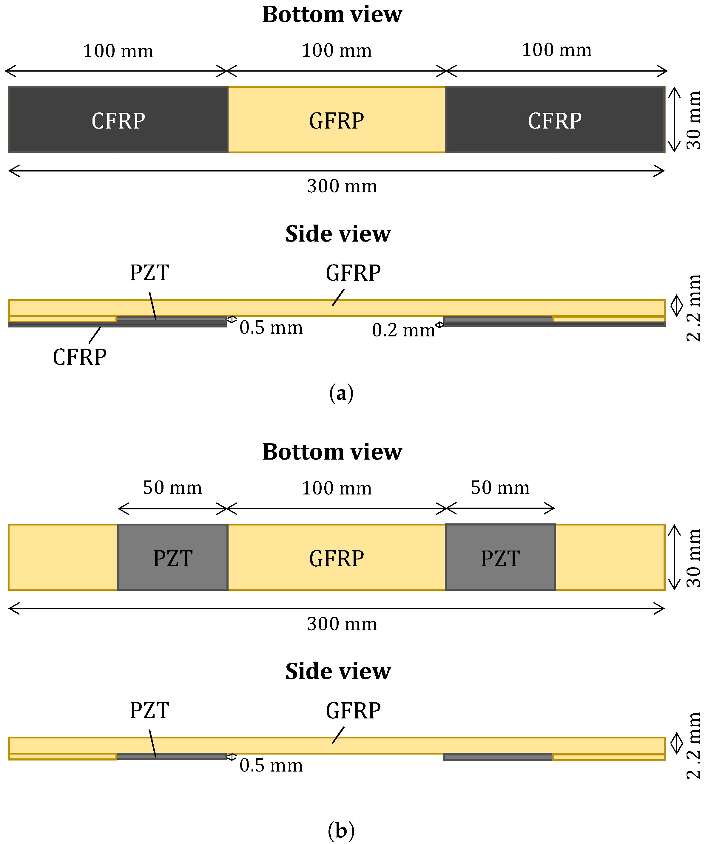
2.2. Beam—Preliminary Study and Fabrication

A narrow composite plate with dimensions 200 × 30 × 2.2 mm3 is studied. The narrow geometry facilitates the excitation of resonance modes that exhibit stress fields similar to those observed in beams. These resonant modes can be analytically represented by the system of Equation (1), with the equivalent properties being the homogenized properties of the composite laminate. Two different designs are explored: an unoptimized configuration and an optimized configuration. The two prototypes are described in Figure 2.
Two PIC 255 piezoelectric actuators, each measuring 50 × 30 × 0.5 mm3, are chosen to actuate the composite plate. These actuators are placed 50 mm from the edges of the beam to allow space for clamping, which was chosen as the boundary condition to facilitate a gradual transition to the final configuration of a clamped leading edge.
For the unoptimized prototype, a GFRP pre-preg composed of glass fibers embedded in an epoxy resin matrix is selected (HexPly 8552-4HS). For the optimized sample, an additional layer of CFRP pre-preg (HexPly 8552-AS4) covers the piezoelectric ceramics. As shown in Figure 2a, the optimized prototype will, therefore, present an additional ply of CFRP for a total length of 100 mm on both sides, from the edge to the end of the piezoelectric actuators, to ensure good clamping in the adopted setup. The mechanical properties of the fiber and matrix components for both pre-pregs are listed in Table 1, where subscripts m and f denote the matrix and fiber properties, respectively.
An optimization study based on an analytical model of the structure was implemented on Python. The objective is to optimize the material thicknesses so that the axes associated with the elastic and inertial forces are aligned. For this purpose, the objective function to minimize is the offset between the neutral axis and the center of mass axis and two optimization variables are considered: the thickness of the GFRP layer and the thickness of the CFRP layer. The thickness of the piezoelectric actuator is fixed at 0.5 mm due to the limited thickness options of commercially available actuators. The total composite thickness, excluding the piezoelectric actuator, is constrained to 2.5 mm; thus, the total beam thickness is constrained to 3 mm.
The optimization results indicate a GFRP thickness of h G F R P = 2.3 mm and a CFRP thickness of h C F R P = 0.2 mm.
However, considering the available ply thicknesses (0.11 mm for GFRP and 0.28 mm for CFRP) and the requirement for symmetric stacking in the glass fiber layers, a GFRP layer with 20 plies is fabricated, resulting in a total GFRP thickness of h G F R P = 2.2 mm with the following ply disposition: 0°/45°/0°/45°/0°/45°/0°/45°/0°/45°//45°/0°/45°/0°/ 45°/0°/45°/0°/45°/0°. For the CFRP, a single ply oriented at 0° with respect to the beam’s longitudinal axis is used. The equivalent properties of the two materials, calculated with the equations presented in the previous section, are then calculated and reported in Table 2. This configuration results in an offset between the two neutral axes of only 0.06 mm, which is considered satisfactory for the optimization. In the absence of the carbon fiber layer, the offset between the neutral axes increases to approximately 0.2 mm, further emphasizing the role of the CFRP layer in achieving the desired decoupling.
Finally, with this material and ply arrangement selection, GFRP pre-preg can have a similar E / ρ ratio to that of ice, with a relative ratio ( ( E / ρ ) s u b s t r a t e / ( E / ρ ) i c e ) of approximately 1.2 and CFRP pre-preg, with a relative ratio of 4.3, combined with soft piezoceramics, with a relative ratio of 0.8, allows achieving an average ratio similar to that of ice.

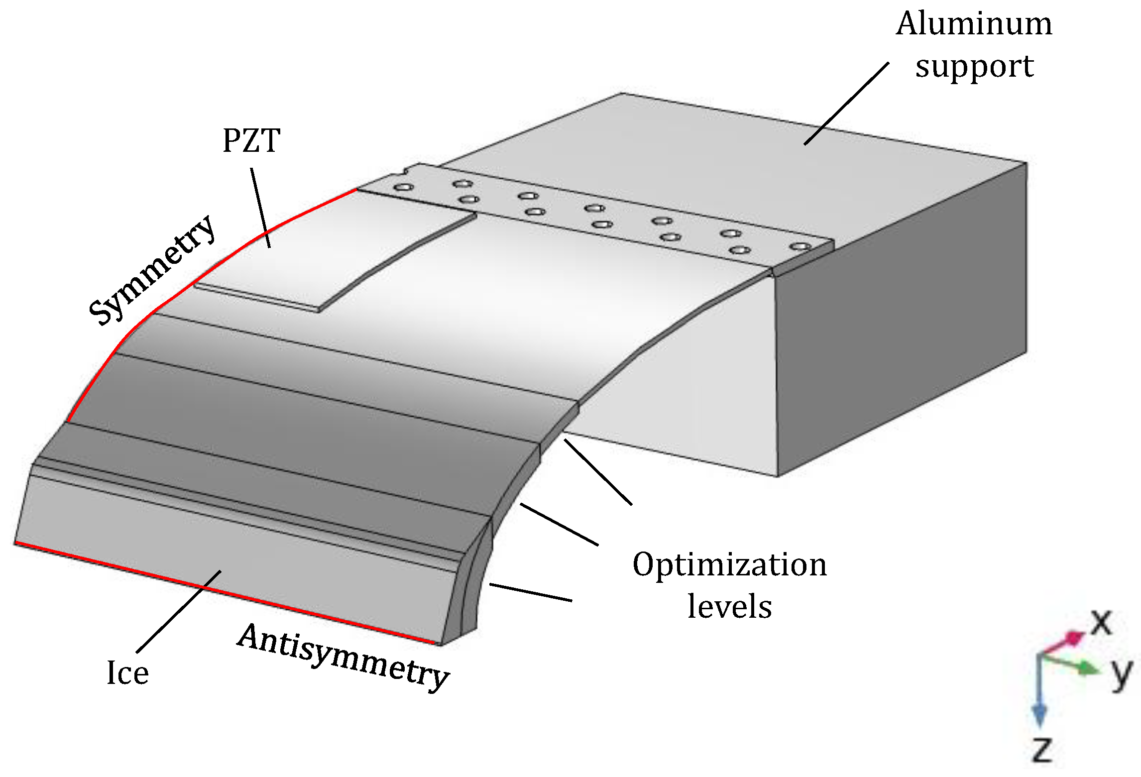
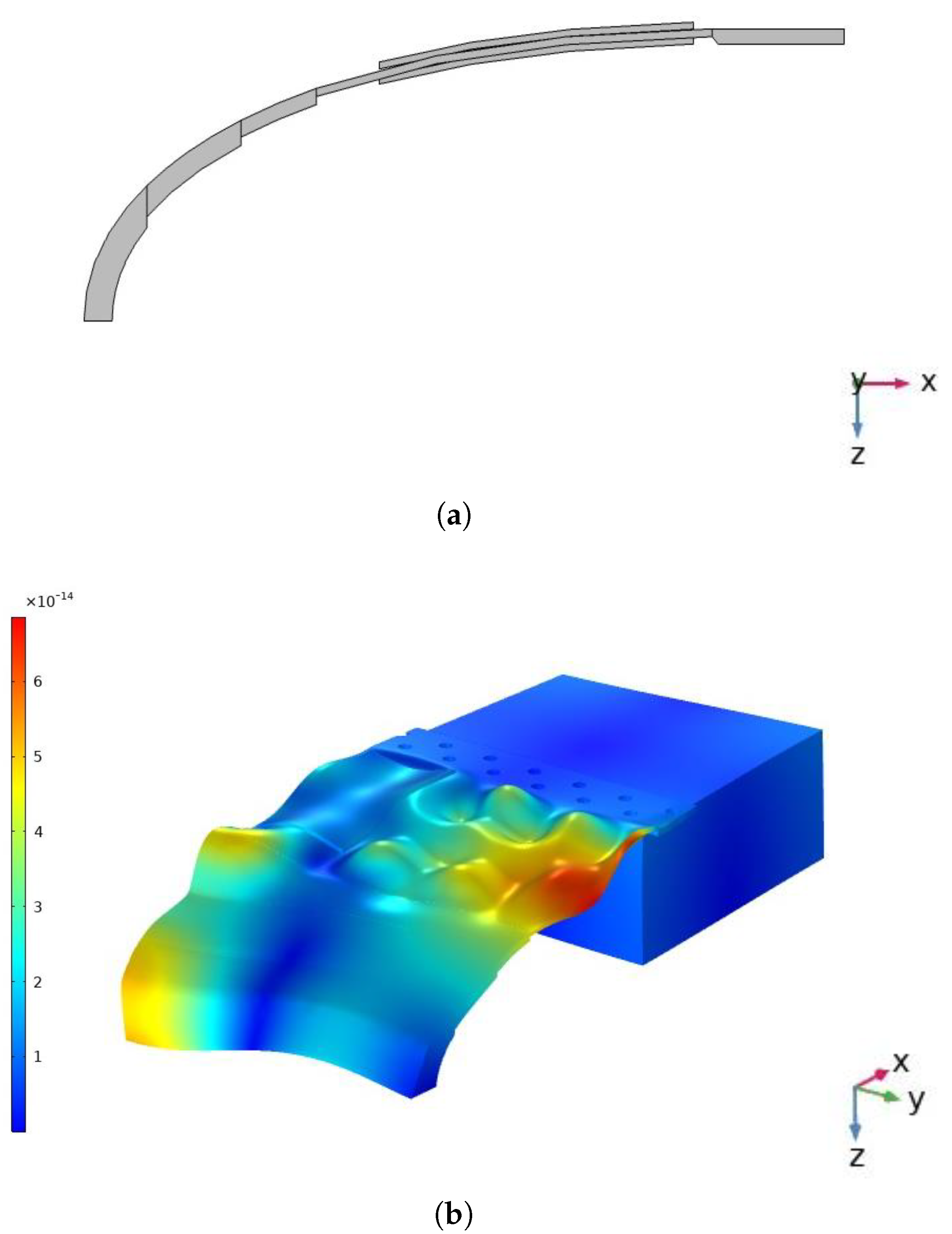
2.3. Curved Composite Structure Study

The origin of the coupling between extensional and flexural modes in curved beams is investigated by studying the analytical wave equations of the system, derived using the Euler–Lagrange formulation.

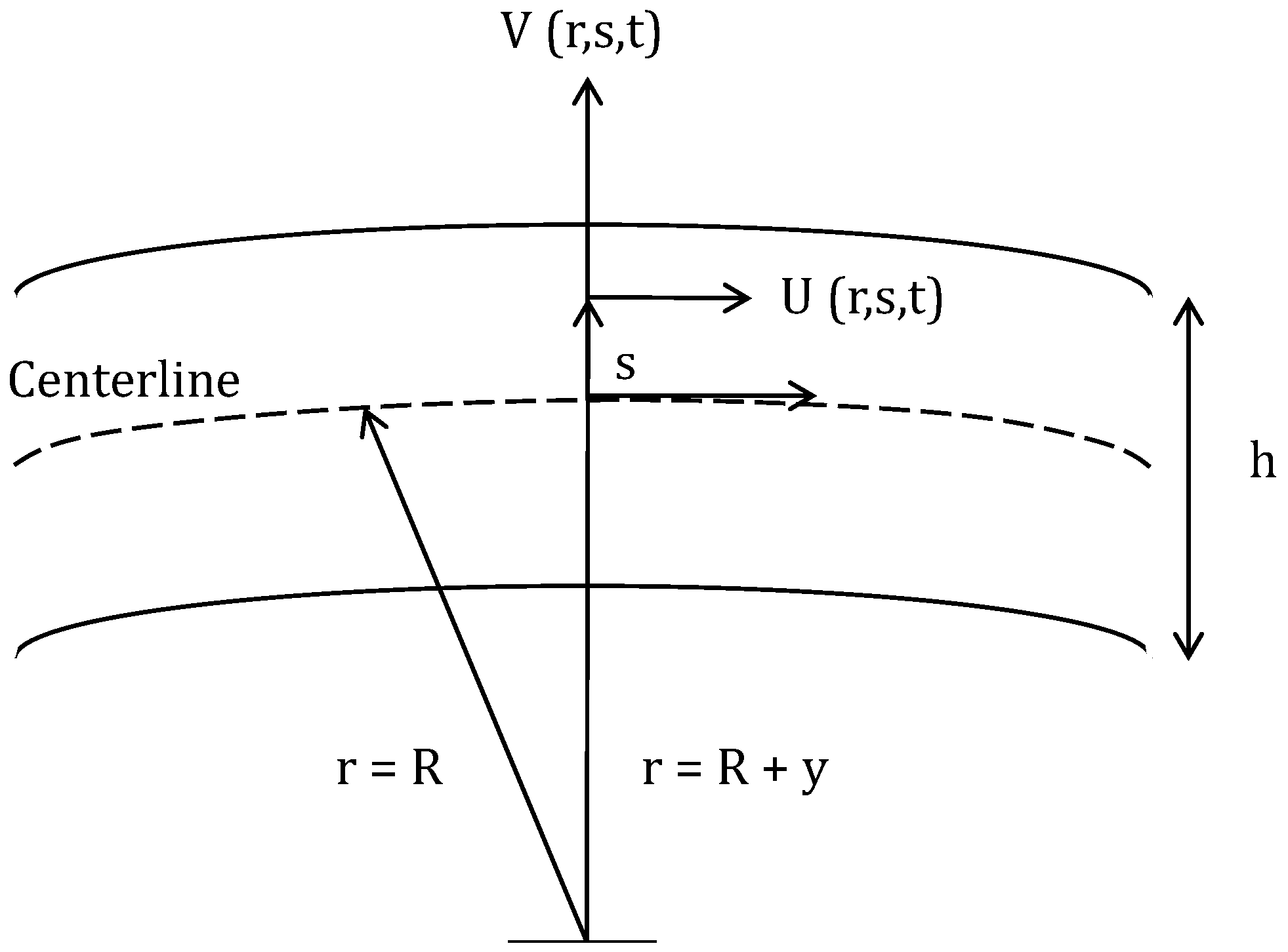
2.3.1. Coupled Wave Equations

Consider a portion of a curved beam (Figure 3). The circumferential coordinate measured along the centerline is denoted as s. The coordinate y represents the normal distance from the centerline, while r denotes the general radial coordinate. For any material point within the beam, the tangential displacement is represented by U ( r , s , t ) , and the radial displacement is denoted by V ( r , s , t ) . These displacements are functions of the radial coordinate r, the circumferential coordinate s, and time t.
The total displacements can be expressed as follows:
U ( r , s , t ) = u ( r , s , t ) + y ϕ ( s , t )
V ( s , t ) = v ( r , s , t )
where u and v are displacement components at the centerline in the tangential and radial directions, respectively. The variable ϕ denotes the rotation of the normal to the centerline as the beam undergoes deformation ϕ = u R v s = u R v s (to simplify the writing of equations, the following notations will be used for the first and second derivatives: f x = f x and 2 f x y = f x y , and for the time derivative f t = f t ). Note that V ( r , s , t ) is independent of y and is completely defined by the centerline component v ( r , s , t ) .
As previously mentioned, the aim is to derive the wave equations using the Euler–Lagrange formulation, which is based on the Lagrangian function.
L ( x , t ) = E k E p = L d d s
where E k is the kinetic energy of the system and E p is its potential energy. They are defined as follows:
E k = 1 2 ( U t 2 + V t 2 ) d m
E p = 1 2 E ε 2 d V
By substituting U t 2 + V t 2 into Equation (6), and considering the assumption that the radius of curvature R is significantly larger than the beam’s thickness, the following equation is obtained:
E k = 1 2 ρ ( U t 2 + V t 2 ) d A d s = 1 2 ρ A ( u t 2 + v t 2 ) + 1 2 ρ I v s t 2 ρ k y + ρ I R u t v s t d s
where ρ A = ρ d A is the axial inertial mass, ρ k y = ρ y d A represents the coupling coefficient, with k y being the first moment of area, and ρ I = ρ y 2 d A is the rotational inertia. In this expression, the kinetic energy of rotation 1 2 ρ I v s t 2 can be neglected.
Similarly, substituting ε 2 into the potential energy gives the following expression:
E p = 1 2 E A u s 2 + 1 2 E I v s s 2 u s v s s E k y + E I R + E A 2 R 2 v 2 + E A R u s v E k y R v v s s d s
where E A = E d A is the axial stiffness, and E I = E y 2 d A represents the bending stiffness. E k y = E y d A is equal to 0 by the definition of the neutral axis.
By minimizing the Lagrangian, it is possible to obtain the following system of equations:
d d s L d u s + d d t L d u t = 0 ,
L d v + d 2 d s 2 L d v s s d d t L d v t + d 2 d s d t L d v s t = 0
which finally leads to the following:
ρ A 2 u t 2 E A 2 u s 2 + E I R 3 v s 3 ρ k y + ρ I R 3 v s t 2 E A R v s = 0
E A R 2 v E A R u s + E I R 3 u s 3 E I 4 v s 4 ρ A 2 v t 2 ρ k y + ρ I R 3 u s t 2 = 0
The system of equations describes the axial and transverse dynamics of a curved beam, accounting for the effects of curvature, stiffness, and inertia.
In the first equation, ρ A 2 u t 2 is the axial inertia of the beam, while E A 2 u s 2 corresponds to the axial stiffness force arising from in-plane deformation. These two terms also characterize the free motion of a beam under extension. The remaining terms in the first equation describe the coupling effects due to the beam’s curvature: E I R 3 v s 3 is the curvature-induced transverse shear, ρ k y + ρ I R 3 v s t 2 is the inertial coupling term, E A R v s models the influence of curvature on the coupling between axial stiffness and transverse motion.
In the second equation, ρ A 2 v t 2 is the transverse inertial of the beam, and E I 4 v s 4 accounts for the bending stiffness. The two terms generally describe the free motion of a bending beam. Additional terms reflect the curvature effects on transverse dynamics: E k y R 2 v s 2 represents the curvature effect on transverse motion, E A R 2 v models the interaction between axial stiffness and curvature. Finally, the coupling terms are E A R u s which represents the coupling between axial displacement and transverse curvature effects, E I R 3 u s 3 which describes the influence of axial deformation on transverse bending, and ρ k y + ρ I R 3 u s t 2 which accounts for the inertial effects.
These different sources of coupling can be compared using a normalization of Equation (11b). Let us consider the following: s ¯ = s / L ,   t ¯ = t ω ,   u ¯ = u / u 0 ,   v ¯ = v / v 0 , where L is the arc length ( L = R α ), u 0 and v 0 are the maximum displacements of the beam for in-plane and out-of-plane motion, respectively. Equation (11b) then becomes the following:
v 0 [ 4 v ¯ s ¯ 4 + E A L 4 E I R 2 v ¯ + ρ A ω 2 L 4 E I 2 v ¯ t ¯ 2 ] = u 0 ρ k y + ρ I R ω 2 L 3 E I 3 u ¯ t ¯ 2 s ¯ A L 3 I R u ¯ s ¯ + L R 3 u ¯ s ¯ 3
The following dimensionless numbers characteristic of the extensional/flexural coupling appear:
π 1 = L R
π 2 = A L 3 I R 12 L 3 h 2 R > > π 1
π 3 = ρ k y + ρ I R ω 2 L 3 E I ρ k y L ρ I < 12 L h
where the angular frequency can be approximated by the following expression ω 1 L E ρ , which itself can be derived from a normalization of the extensional wave equation. An analysis of orders of magnitude, which is conducted by considering a rectangular cross-section, shows that the curvature effects associated with π 2 are the dominant factor in the generation of parasitic flexion.

2.3.2. Coupling Analysis with Rayleigh Method
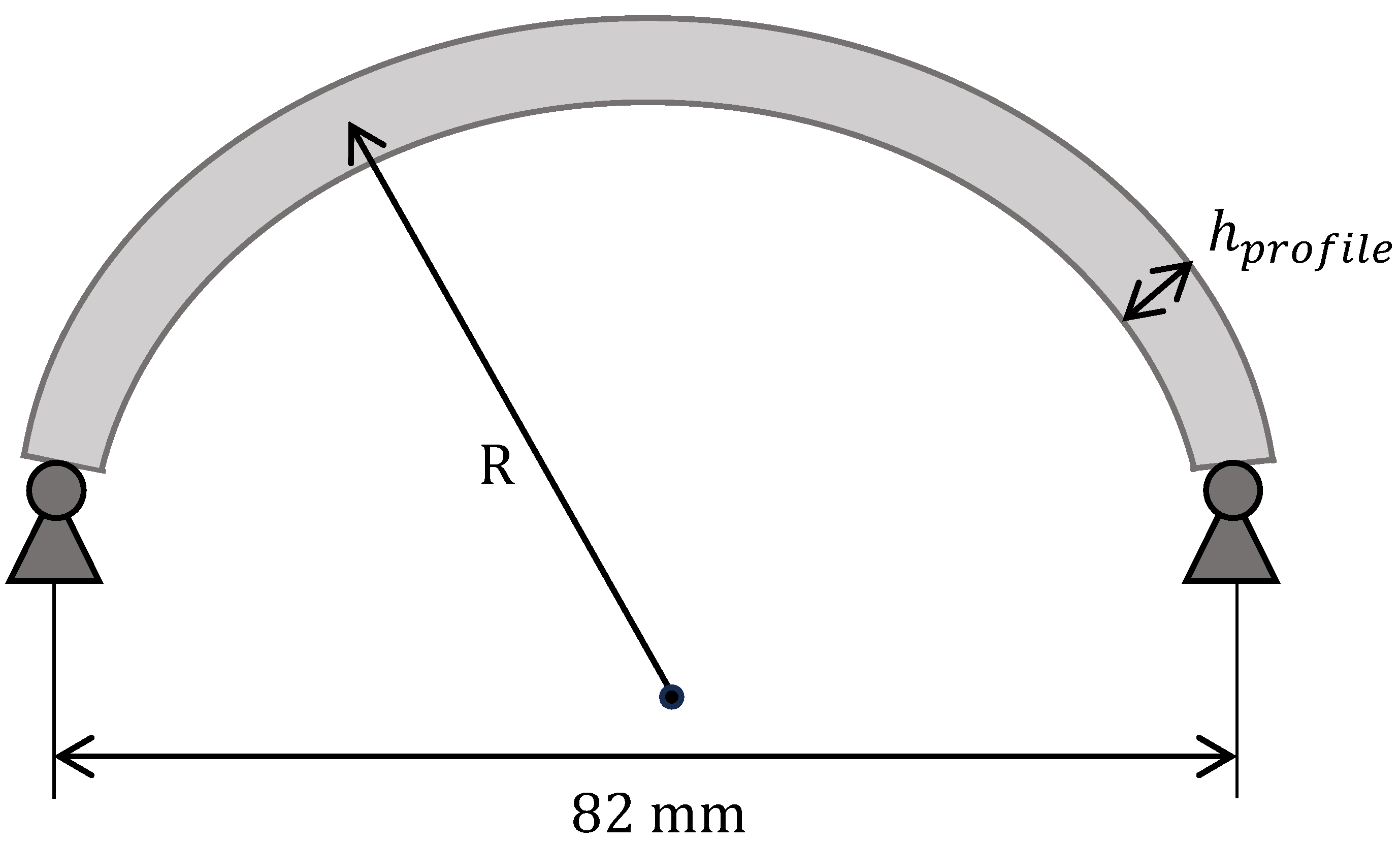
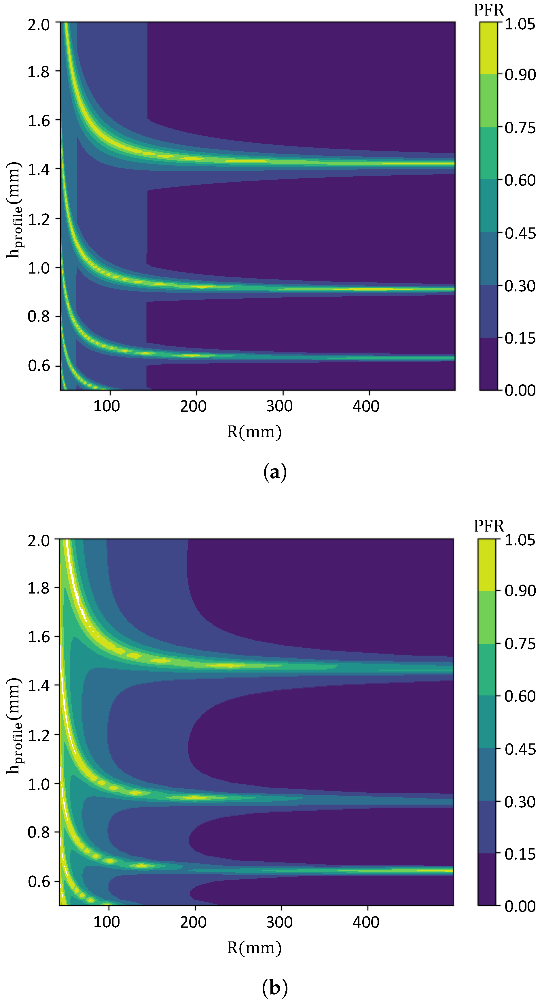
The Rayleigh method is used to approximate the angular frequency ω and analyze the coupling between flexural and extensional modes [30]. Again, the beam is considered under pinned-pinned boundary conditions at its edges. The in-plane and out-of-plane displacements are expressed as follows:
U ( s , t ) = u 0 s i n ( π s L ) s i n ( ω t )
V ( s , t ) = v 0 s i n ( n π s L ) s i n ( ω t )
Let us consider the assumption of an isotropic material and a constant radius of curvature R ( ρ k y = 0 and E k y = 0). Substituting U ( s , t ) and V ( s , t ) into Equation (8), the maximum kinetic energy can be written as follows:
E k = 1 2 ρ A ω 0 2 u 0 2 s i n 2 π s L + v 0 2 s i n 2 n π s L ρ I R u 0 v 0 ω 0 2 n π L s i n π s L c o s n π s L d s = ω 0 2 ρ A L 4 ( u 0 2 + v 0 2 ) ρ I R C k n u 0 v 0
with
C k n = n 2 1 + ( 1 ) n ( n + 1 ) 1 + ( 1 ) n ( n 1 )
Similarly, substituting U ( s , t ) and V ( s , t ) into Equation (9), the maximum potential energy can be written as follows:
E p = [ E A 2 π 2 L 2 u 0 2 c o s 2 π s L + E I 2 v 0 2 n π L 4 sin 2 n π s L + E A R π u 0 v 0 L cos π s L sin n π s L = π 2 4 L E A u 0 2 + n 4 π 4 4 L 3 E I v 0 2 + E I 2 R u 0 v 0 ( n π L ) 2 C p n + E A L 4 R 2 v 0 2 + E A 2 R u 0 v 0 C p n
with
C p n = 1 + ( 1 ) n ( n + 1 ) + 1 + ( 1 ) n ( n 1 )
The equality of the two energy contributions enables the computation of the Rayleigh quotient represented by ω 0 2 :
ω 0 2 = π 2 4 L E A u 0 2 + n 4 π 4 4 L 3 E I v 0 2 + E I 2 R ( n π L ) 2 C p n u 0 v 0 + E A L 4 R 2 v 0 2 + E A 2 R u 0 v 0 C p n ρ A L 4 ( u 0 2 + v 0 2 ) ρ I R C k n u 0 v 0
Equation (22) can be written as a function of the parasitic flexural ratio α = V 0 U 0 :
ω 0 2 = a α 2 + b α + c d α 2 + e α + f
where
a = n 4 π 4 4 L 3 E I + E A L 4 R 2 , b = E I 2 R n π L 2 C p n + E A 2 R C p n c = π 2 4 L E A , d = ρ A L 4 e = ρ I R C k n , f = ρ A L 4
To approximate the angular frequency, Equation (23) is minimized with respect to α , which results in the following:
a e b d α 2 + 2 a f 2 c d α + b f c e = 0
Once Equation (25) has been solved, the parasitic flexural ratio α can be calculated, as well as the angular frequency ω 0 .

2.3.3. Case Study

A curved profile with a constant curvature, as depicted in Figure 4, is studied. This profile is assumed to be made of a glass fiber-reinforced polymer with homogeneous mechanical properties.
Figure 5 illustrates the variation in the parasitic flexural ratio (PFR) as a function of the profile’s geometric properties, specifically its radius and thickness, using both numerical and analytical methods. The analytical PFR is derived by solving Equation (25), while the numerical PFR is obtained through Finite Element Analysis conducted with Ansys, in conjunction with Matlab. As shown in Figure 5, the proposed analytical approximation aligns well with the numerical results. Although the analytical formulation requires a series of calculations, it offers significant advantages. Not only does it enable the source of parasitic flexion to be analyzed, but it also considerably reduces calculation time. While generating the PFR map using numerical methods requires approximately 27 h (on a LENOVO PC with an Intel Core i7 2.3 GHz, 16 GB RAM processor), the analytical approach achieves the same result in only 44 s, underscoring its computational efficiency.
This study provides important conclusions regarding the mitigation of parasitic flexion when the curvature radius R decreases. Figure 5 shows that there are zones, highlighted in yellow, which correspond to high values of PFR and which must then be avoided. These zones do not correspond to constant values of thickness, and therefore, unlike in the case of beams and plates, it is not sufficient to use a material with a similar E / ρ ratio to that of ice to mitigate parasitic flexion. The substrate thickness must also vary along the profile to maintain a low PFR. For smaller radii ( R < 100 mm), the h p r o f i l e must be progressively increased to maintain low PFR values. For profiles with larger radii ( R > 100 mm), the PFR is independent of the radius R and three critical thickness values h c i = 0.64 , 0.92 , 1.48 mm exhibiting high PFR are identified within the studied thickness range and must be avoided.
This conclusion has important implications for practical applications. For example, when addressing the issue of the leading edge of a profile characterized by a variable curvature, where the radius decreases progressively toward the nose, a gradual increase in the substrate thickness can be employed to mitigate parasitic flexion. This strategy will be applied to a leading-edge prototype in the following section.

3. Results and Discussion

3.1. Beam—Numerical Study and Experimental Validation

3.1.1. Numerical Study

Numerical analyses are performed for a beam in clamped boundary conditions to evaluate the parasitic flexural ratio for both the optimized and unoptimized samples. A uniform glaze ice layer is modeled at the center of the beam, having a total length of 100 mm, a width of 30 mm, and a thickness ranging from 2 to 4.5 mm. The first extensional mode is found at a frequency of around 15.9 kHz and 15 kHz for the optimized and unoptimized beam, respectively. The results are presented in Table 3. The optimized design results in a consistently lower PFR than that of the unoptimized beam. It is possible to notice that the PFR is above the predefined limit of 0.4 for an ice thickness of 2.5 mm. For h i c e = 2.5 mm, the PFR for the unoptimized beam is equal to 0.64, whereas for the optimized beam, this value is only 0.27. The respective modal shapes are reported in Figure 6.
Therefore, an ice thickness of 2.5 mm is chosen to compare the de-icing capabilities of the optimized and unoptimized samples.

3.1.2. Experimental Validation

Before performing the tests, the input voltage VG required to activate the fracture mechanism by exceeding the fracture toughness was estimated. This is achieved by rescaling the modal quantities with the critical value of G. The formula has already been mentioned in [31] and is given below.
V G = 2 E ( mod ) q c ( mod ) Q m G c ( ice ) G ( mod-ice )
where E ( mod ) is the modal elastic strain energy of the system, q c ( mod ) is the modal electric charge, Q m is the mechanical quality factor, G c ( ice ) is the toughness at the interface between the ice layer and the substrate, and G ( mod-ice ) is the modal energy release rate.
Given the estimated fracture toughness and quality factor (Gc = 1 J/m2, Qm = 20), the voltages are computed: VG = 191 Vpk for the optimized beam and VG = 212 Vpk for the unoptimized beam. Thus, a value of 200 Vpk is selected for the tests.
After this analysis, the two prototypes were tested. The prototypes were first inserted into the clamping system and then placed inside a freezer maintained at −20 °C. A supercooled water film was poured onto the surface, restricted to an area of 100 × 30 mm2, until a 2.5 mm thick ice layer was formed. The conditioning time was approximately one hour. An electronic caliper (Mitutoyo Absolute AOS Digimatic) was used to verify that the desired ice thickness was achieved. A low-voltage sweep (20 Vpk) was first used to detect the extensional resonant mode. For the optimized prototype, the resonant frequency was identified at 15.7 kHz, and it was then excited at 200 Vpk using both piezoelectric transducers as actuators for a duration of 8 s. The optimized prototype achieves effective de-icing in 2 s, leaving only two small pieces of ice attached to the surface at the extremities of the ice layer (Figure 7). The unoptimized beam reaches a similar de-icing condition in 1.4 s at a frequency of 14.8 kHz, and slightly more ice remains adhered to the surface compared to the optimized configuration (Figure 8). It should be noted that a significant issue arises with the unoptimized beam: after the first de-icing test, one of the piezoelectric transducers failed, a problem not encountered in the optimized beam.

3.1.3. Discussion

The failure of the piezoelectric transducer was examined in more detail. It was hypothesized that stress was the primary cause of this failure. To verify this assumption, the maximum voltage that the piezoelectric actuators could withstand was determined using an FEM analysis as follows:
V p z t = 2 E ( mod ) q c ( mod ) Q m σ c ( pzt ) σ ( mod-pzt )
where σ c ( pzt ) represents the tensile strength of the piezoelectric transducers, which is 30 MPa, while σ ( mod-pzt ) denotes the modal tensile stress in the piezoelectric transducers.
For Qm = 20, it was found that the voltages are Vpzt = 223 Vpk for the optimized beam and Vpzt = 214 Vpk for the unoptimized beam. Notably, the voltages Vpzt and VG for the unoptimized beam were very close, suggesting that parasitic flexion could be a contributing factor to the actuator’s failure. This flexion not only degrades de-icing performance but also significantly increases the stress within the piezoelectric actuators. In the two configurations analyzed, it was determined that the stress on the piezoelectric actuators of the unoptimized beam could be up to 1.2 times higher in certain regions compared to the optimized beam, thus highlighting the necessity of mitigating parasitic flexion during the design of a prototype.

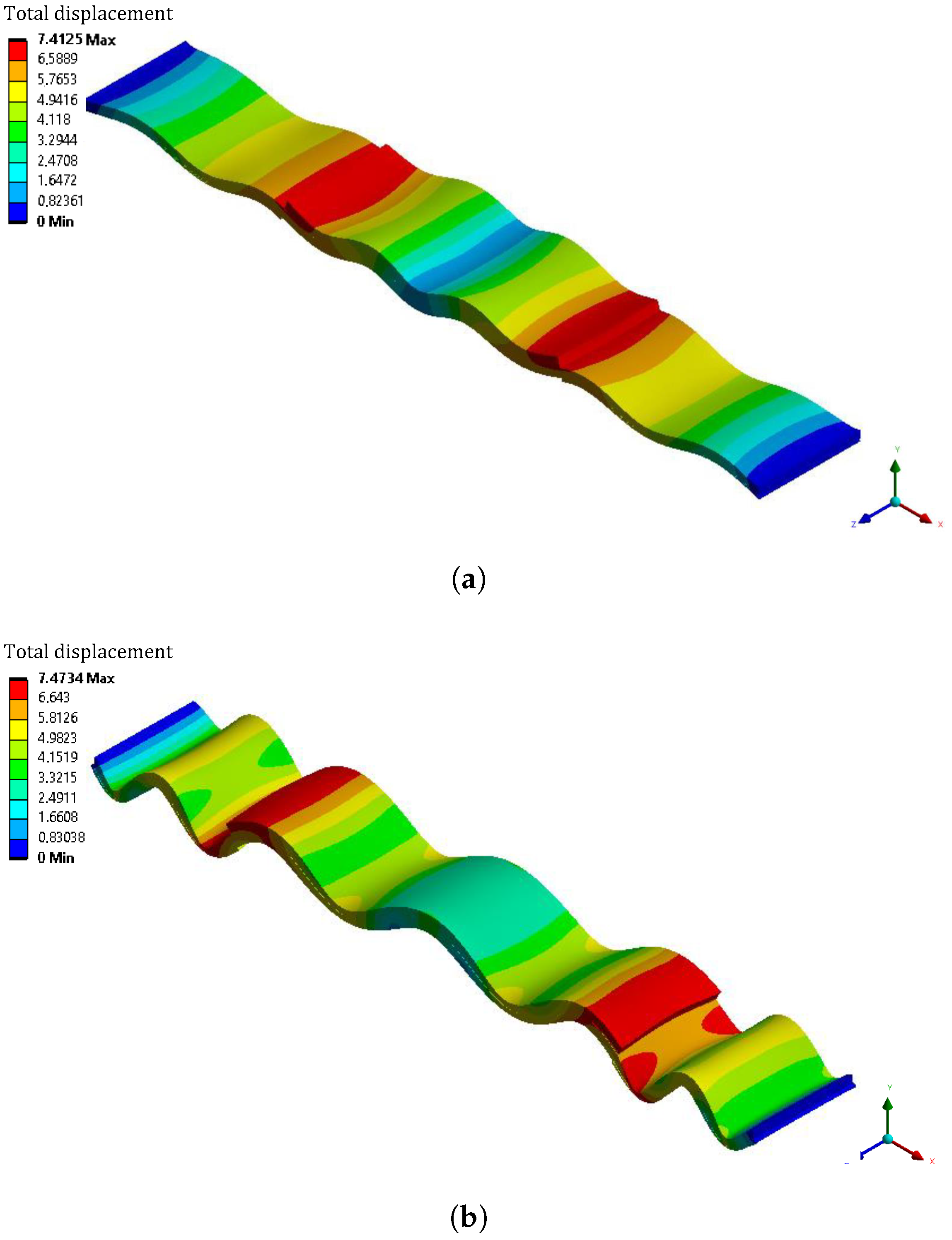
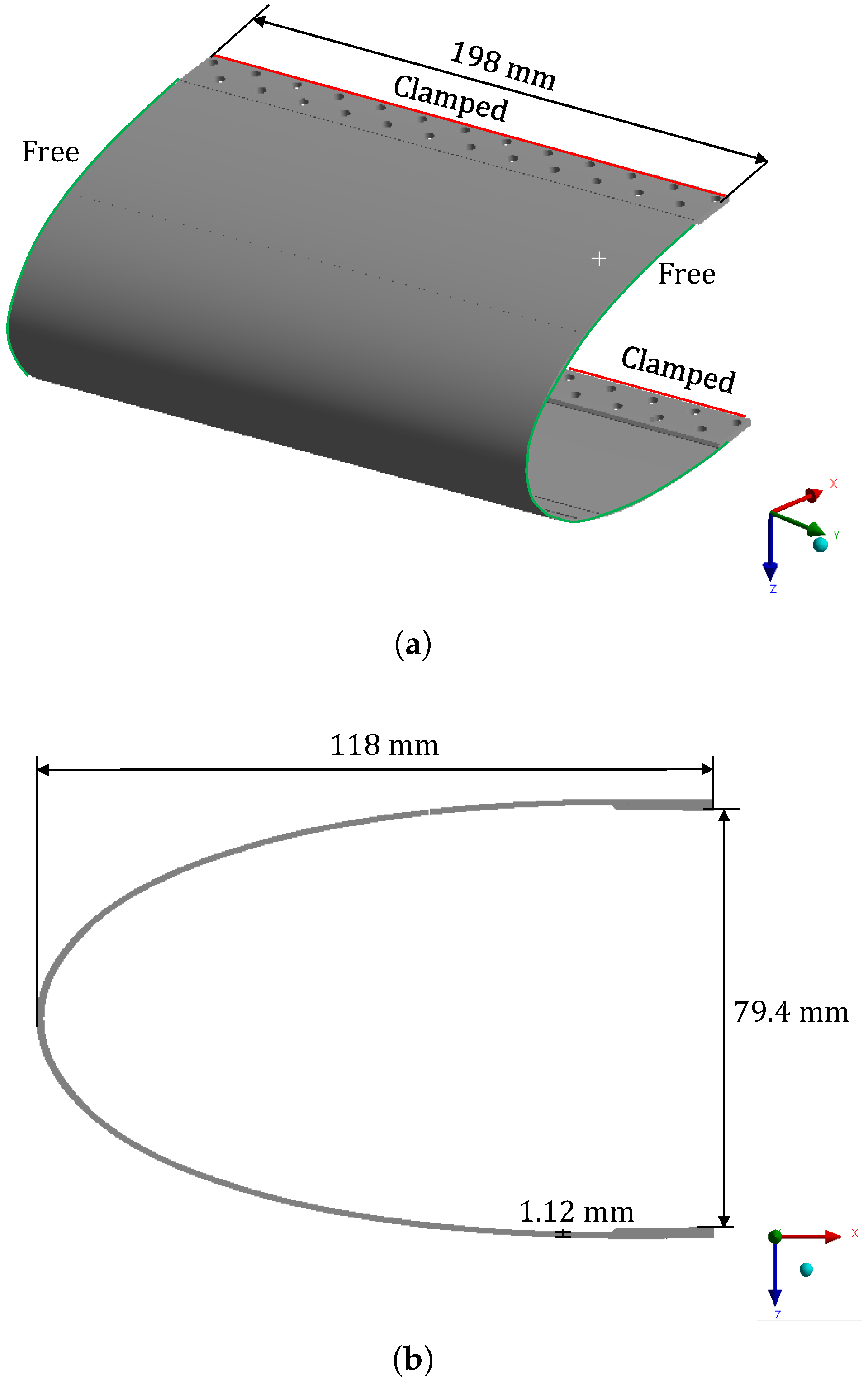
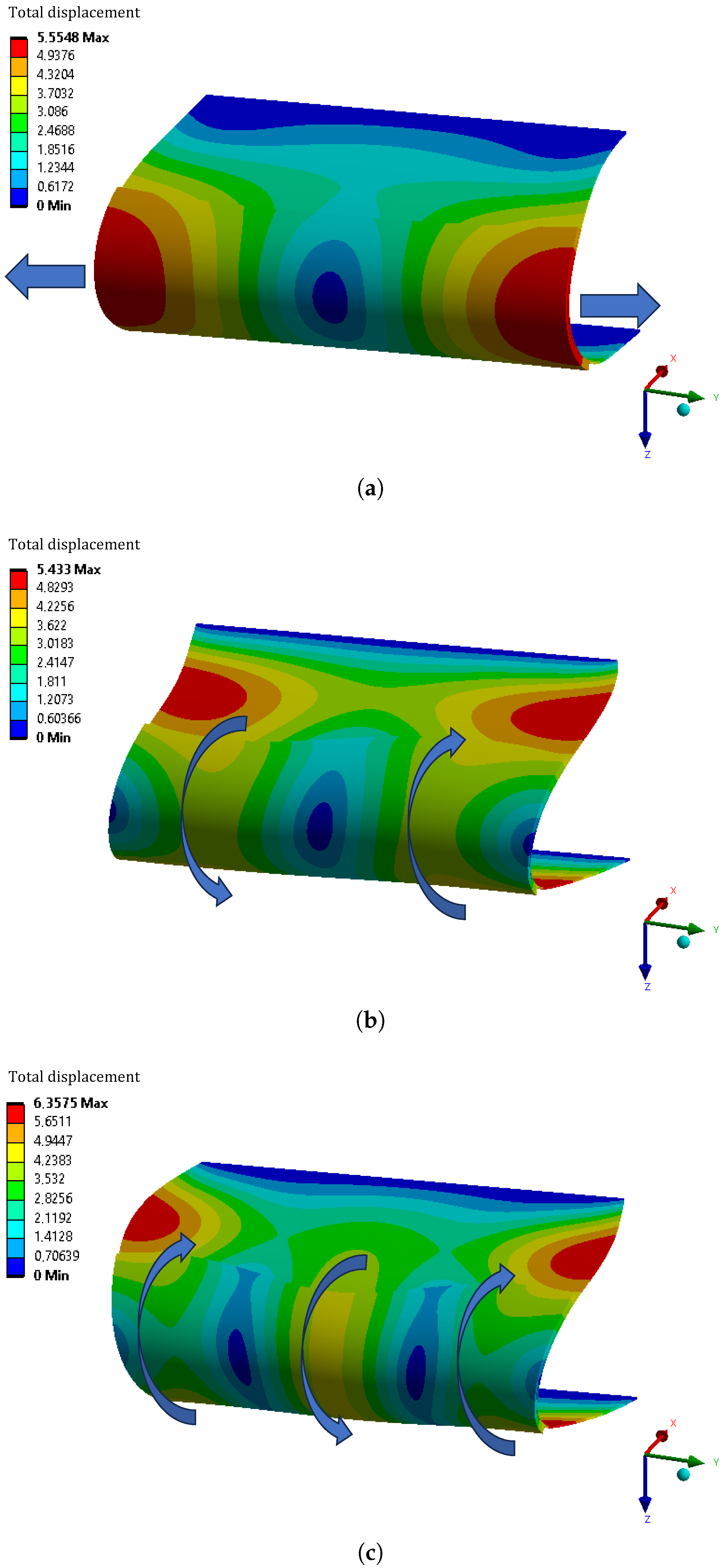
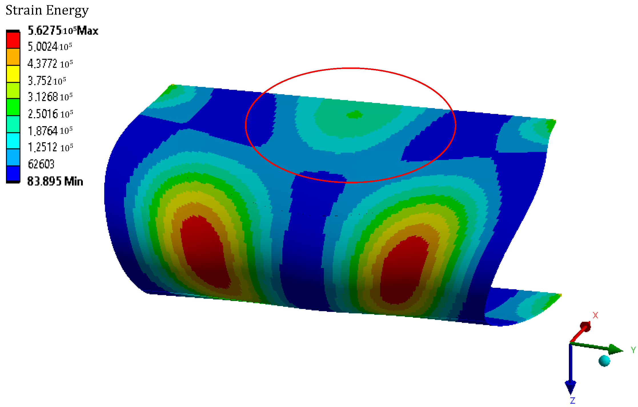
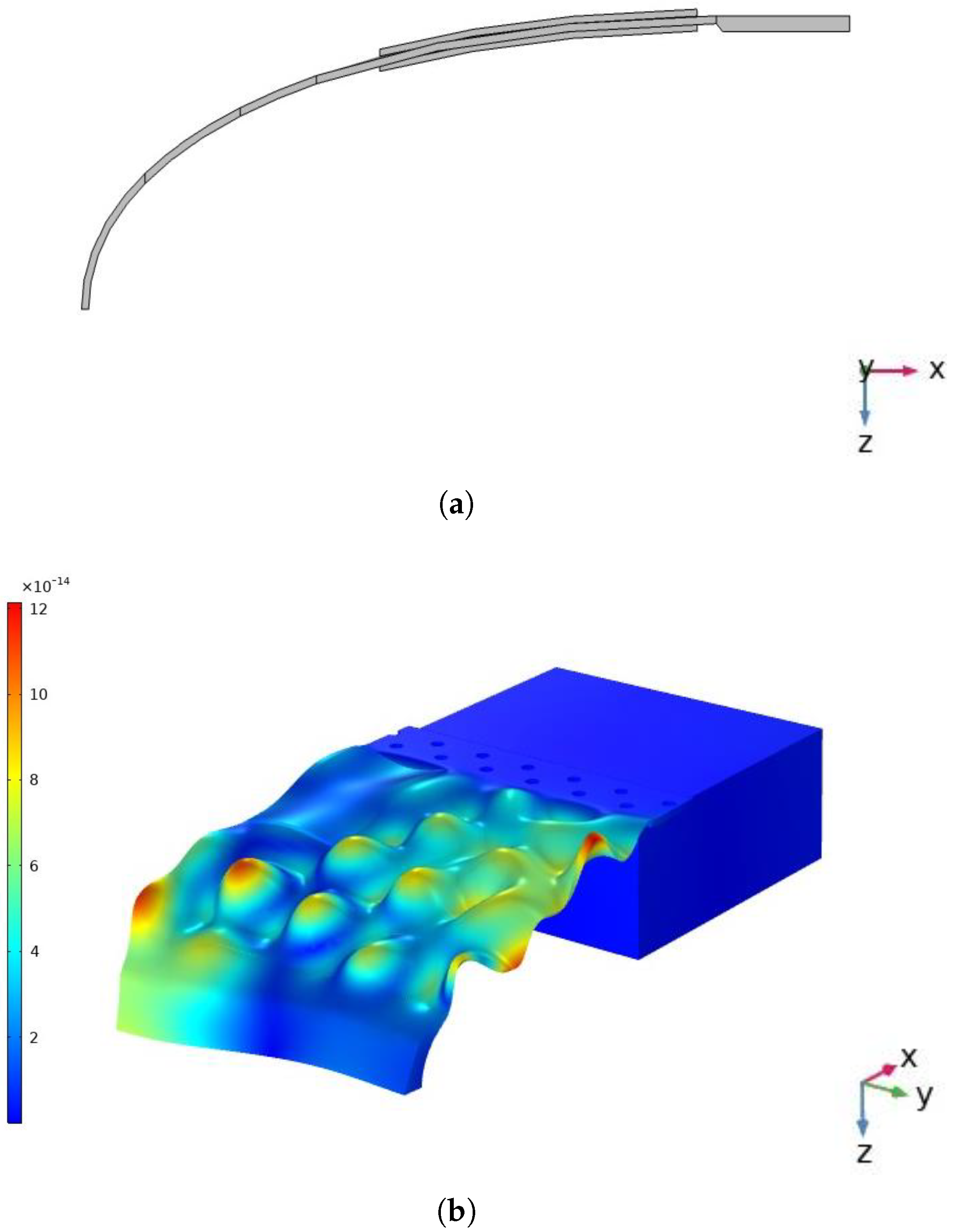
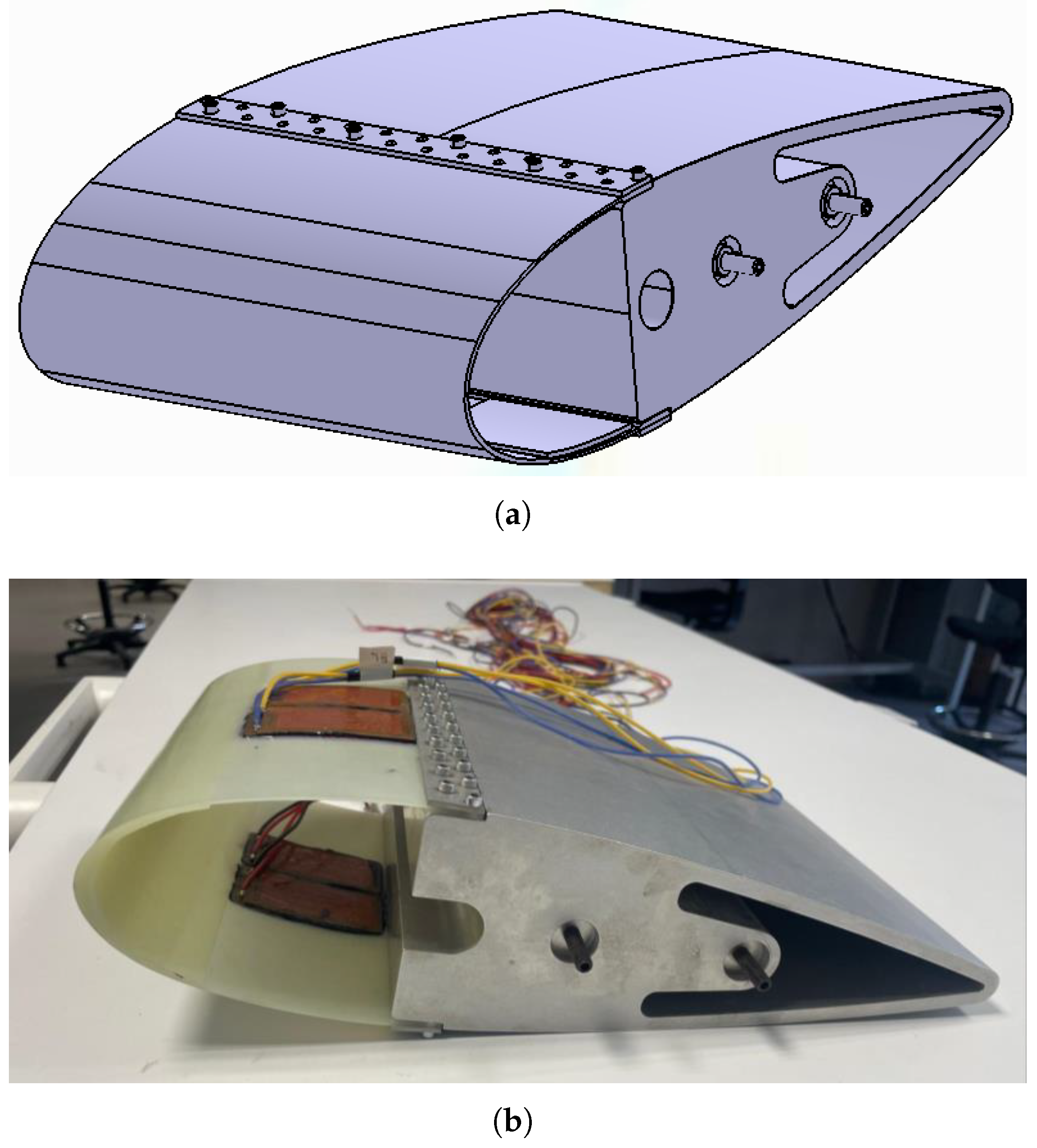
3.2. Leading Edge—Numerical Study and Experimental Validation

The design optimization methodology is applied to a NACA 0024 airfoil leading edge incorporating the optimization strategies learned from a constant-curvature beam. To simplify the analysis, the assumption of a uniform spanwise thickness is considered. Additionally, the edges are assumed to be in free boundary conditions, while the prototype is clamped to an aluminum support. The prototype features the dimensions illustrated in Figure 9. Length measurements are taken along the chordwise (x) direction, while width measurements will correspond to the spanwise (y) direction.

3.2.1. Numerical Study

A 3D analysis is conducted on a clamped NACA 0024 leading edge, modeled with homogenized GFRP material properties, and a uniform 3 mm-thick layer of ice accreted on its surface. A condition to avoid the normal displacement is applied to the substrate’s surface to evaluate the behavior of pure extensional modes. To determine the most suitable mode for this study, the ratio of the elastic energy stored within the ice layer to the total elastic energy of the system is evaluated for three distinct extensional modes, as illustrated in Figure 10.
The calculated energy ratios for the three modes are 0.46, 0.33, and 0.35, respectively. These results indicate that the first extensional mode is theoretically the most effective for de-icing, as it stores the highest amount of energy within the ice layer. However, due to constraints on actuator placement (specifically, the need to position actuators near the clamped edge to avoid the high curvature at the front of the leading edge), the first mode cannot be effectively excited. Therefore, the third extensional mode (Figure 10c) is selected for this study.
To further analyze the energy distribution, the energy ratios for the three resonant modes were recalculated using the same numerical model but substituting the glass fiber composite substrate with an aluminum alloy. They are 0.21, 0.16, and 0.18, respectively. These results demonstrate that the energy ratios are consistently lower when an aluminum substrate is used, indicating that the elastic energy stored in the ice layer is reduced for aluminum substrates when the same mode is excited. This observation highlights the advantages of using GFRP substrates combined with electromechanical resonant de-icing systems.
The placement of the DuraAct P-876.A15 piezoelectric actuators is evaluated via a preliminary numerical analysis on a reference leading edge. The actuators are modeled by pair, and each pair is considered as a single 1 mm-thick piezoelectric actuator. In general, the actuators must be positioned near the clamped edges to minimize exposure to regions with high curvature. Additionally, they should be located in areas where the mode exhibits high energy density, as this ensures effective coupling between the actuators and the structure. As illustrated in Figure 11, the region with the highest energy density for the considered mode is located at the center of the prototype. Consequently, two pairs of actuators are positioned in this central region. To maintain the balance of the neutral axis in this area, the actuators are placed on both the inner and outer surfaces of the prototype.
The optimization analyses are conducted using COMSOL Multiphysics, chosen for its ease of use for complex designs of experiments. To improve computational efficiency, only one-quarter of the geometry is modeled. Symmetric boundary conditions are applied along the y-axis, while an antisymmetry condition is placed along the z-axis to correctly obtain the desired mode. The model includes an 18-mm-long tab with holes designed to allow assembly with the aluminum support. The aluminum support is represented numerically as a rectangular mass with dimensions of 99 mm half-width, 39.7 mm half-height, and 90 mm length, and the two bodies are considered bonded. The edges of the leading edge are modeled with free conditions.
The shape of the ice layer is also modified to be more coherent with the ice deposits realized in the icing wind tunnel. Numerically, the ice is still considered high-density glaze ice (E = 9 GPa, ρ = 900 kg/m3). The meshing is conducted with tetrahedral elements, and a more refined mesh is used for the prototype, actuators and ice layer to ensure the accuracy of the results, while a coarser mesh is used for the aluminum support to reduce the computational time. The model is reported in Figure 12.
An unoptimized composite leading edge is considered first. The number of plies chosen for this structure is 4. The considered material is once more HexPly M34, which has a single-ply thickness of 0.28 mm. The ply stacking sequence is 0°/45°/−45°/0°, resulting in a total laminate thickness of 1.12 mm. Based on the ply arrangement and orientation, the calculated equivalent mechanical properties are E = 18.62 GPa and ρ = 1799 kg/m3.
In Figure 13b, the extensional mode is found at a frequency of 14.4 kHz for the unoptimized leading edge, and it is possible to notice that the mode is coupled with parasitic flexion. Two different parasitic flexural ratios are calculated: the global PFR (PFRtot), which is the ratio of the maximum normal displacement divided by the maximum tangential displacement, and the local PFR in the iced area (PFRice), which is ultimately the one that is important to de-ice the structure. The values for the unoptimized leading edge are PFRtot = 1.79 and PFRice = 0.7. Even by balancing the neutral axis of the actuators and using a material that has an equivalent E / ρ close to that of ice, it is possible to notice that, as predicted by the analytical equations, the curvature effect induces parasitic flexion. It is, therefore, necessary to assess whether it is feasible to reduce the PFR, particularly in the iced area, by designing an optimized leading edge with a thickness that varies along the chord.
An optimized leading edge is designed by adding layers of GFRP plies to the curvature of the leading edge, resulting in an increased thickness in this area. The width of the layers is the same as that of the leading edge. The length of each additional layer varies, resulting in a non-uniform thickness along the chord. The initial layer is the longest, and the subsequent layers are progressively shorter, with lengths of 96.3 mm, 70.9 mm and 36.7 mm, respectively. These values have been selected based on the projected length x. The projected lengths of the layers are 37 mm for the first, 25 mm for the second and 10 mm for the third. Initially, the difference between the projected lengths was supposed to be 10 mm, 15 mm and 15 mm. However, to better accommodate the positioning of the piezoelectric actuators, the first difference was adjusted to a Δ x of 12 mm.
The final design of the optimized profile is achieved thanks to a design of experiments based on the variation of the following parameters: the number of plies in each layer, ranging from 0 to 4, and the maximal thickness of the ice layer on the leading edge stagnation point, fixed at 3.5 mm, 4.75, and 6 mm.
A full-factorial design of experiments is employed to explore all possible combinations, resulting in a total of 375 configurations. To determine the most effective optimized configuration, two key parameters are evaluated: the parasitic flexural ratio PFRice, and the voltage required to de-ice. The de-icing voltage is calculated with Equation (26), with a toughness value of Gc = 0.5 J/m2 and a quality factor Qm of 30. Based on these criteria, the optimal configuration consists of four plies in each additional layer (see Figure 14a). With an ice layer with a maximum thickness of 6 mm, the calculated value of PFRice is 0.11, and the required de-icing voltage is 235 V. Additionally, PFRtot is significantly reduced, with a value of 0.72 in the rear part of the leading edge.
For thinner ice layers, the required de-icing voltage increases to 319 V for a maximum thickness of 4.75 mm and 500 V for 3 mm, while the parasitic flexural ratio remains relatively stable at 0.13 and 0.15, respectively. This demonstrates that the optimization effectively reduces parasitic flexion across a range of ice thicknesses. However, the required voltages remain relatively high. Given the limitations of the available laboratory power supply, experimental testing is feasible only for configurations with a maximum ice thickness of approximately 6 mm. The optimized mode is presented in Figure 14b.

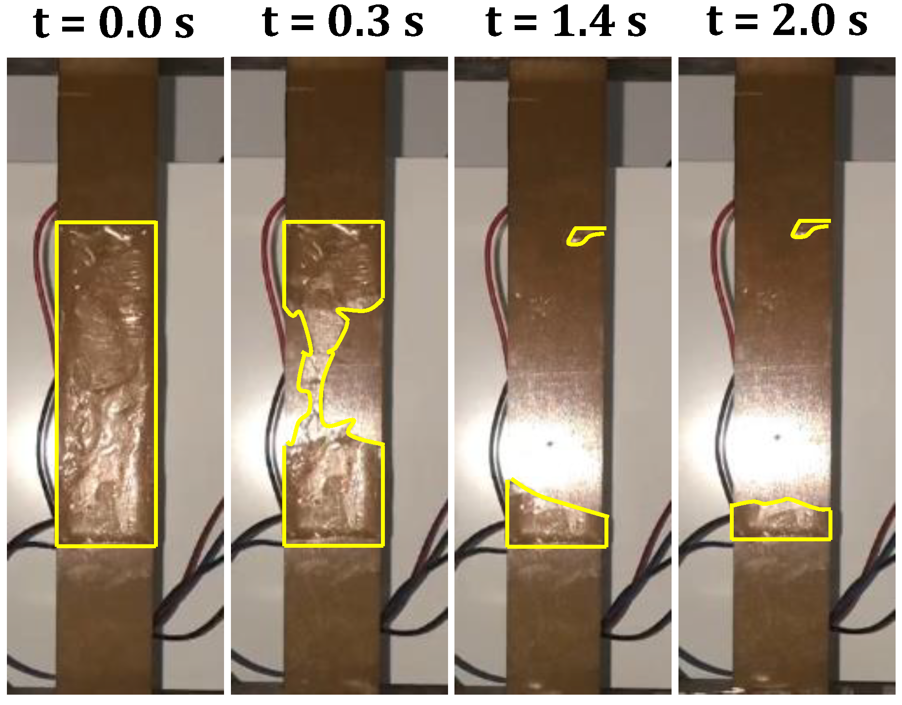
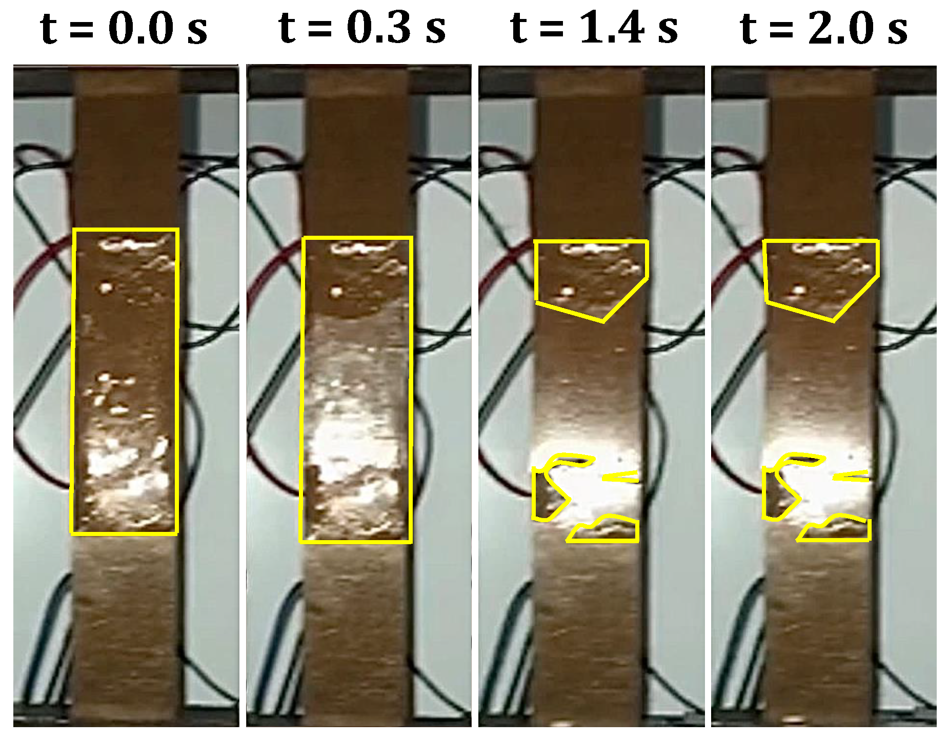
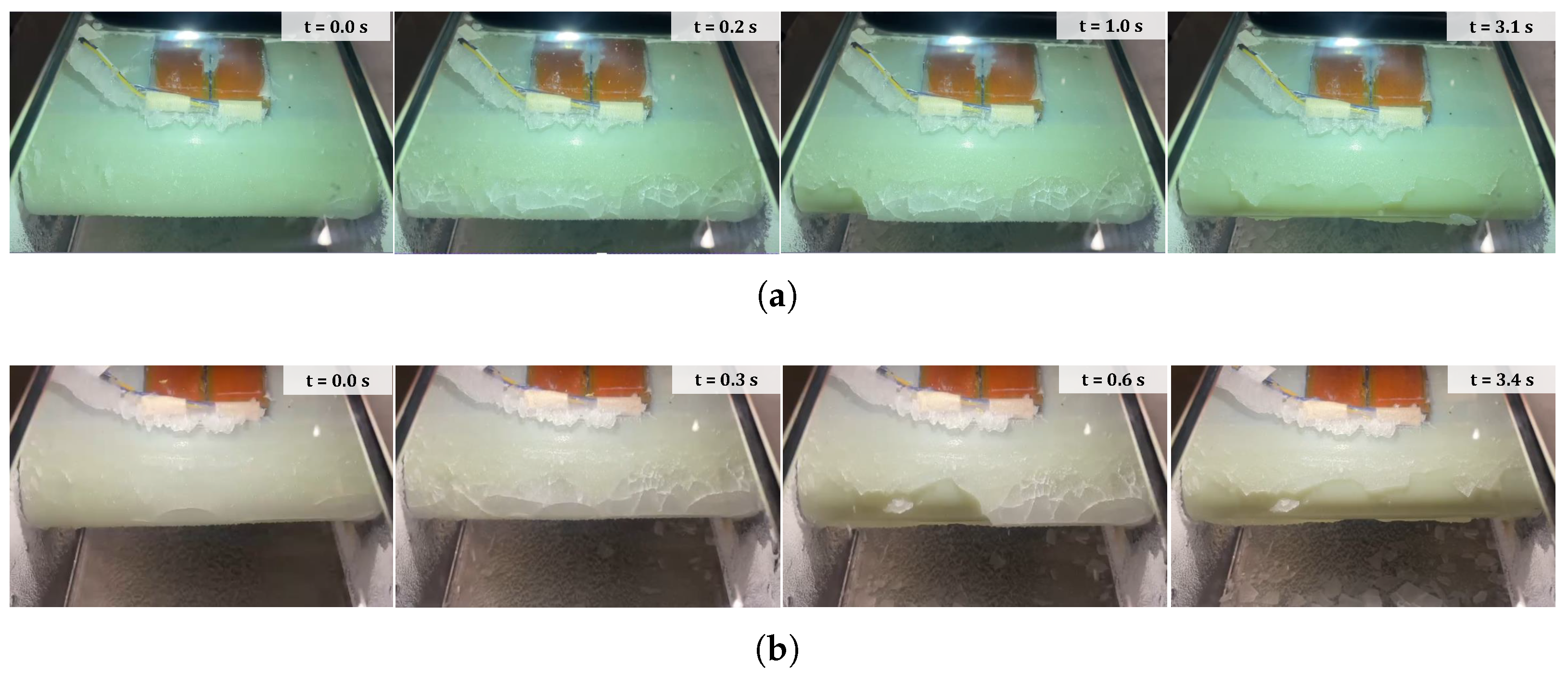
3.2.2. Experimental Validation

The prototype was then positioned in the icing wind tunnel to evaluate its de-icing performance. The aluminum support on which the prototype was mounted was custom-designed for installation in the tunnel. The prototype was clamped using two rows of hexagon socket M3 screws. The airfoil had a total chord length of 330 mm, a width of 198 mm, and a maximum thickness of 83.5 mm. The CAD model and the final prototype are shown in Figure 15.
Once the prototype was placed into the icing wind tunnel, the ice deposit was performed with the double injector system. To better control the temperature, multiple ice deposits were conducted around a temperature of −2.5 °C. The velocity was set around 18 m/s, the MVD was 50 μ m, and the LWC ranged from 1 to 10 g/m3. A total of eight deposits of 40 s each were performed to obtain the desired maximum ice thickness of around 6 mm. A clear, glazed ice layer was obtained.
A low-amplitude identification sweep (6 Vpk) was conducted to prevent the formation of fractures in the ice prior to the de-icing process. The resonant frequency was determined to be 14.46 kHz, which aligns well with the numerical model prediction of 14.81 kHz. At this voltage, a quality factor Qm of 17 was measured.
One of the piezoelectric transducers was found to be non-functional due to an issue that arose during the welding of cables to the electrodes. Additionally, a prior high-voltage sweep at 100 Vpk may have contributed to the malfunction. Consequently, only 15 out of the original 16 actuators were operational. The de-icing voltage was increased to compensate for the loss of functionality in the faulty actuator and to account for a lower than expected Qm factor. When the required voltage was recalculated using a Qm factor of 17 instead of the initial 30, the estimated voltage requirement increased to 415 Vpk. Unfortunately, this voltage exceeded the capabilities of the available power supply and the voltage was limited to 300 Vpk for testing.
The 300 Vpk de-icing chirp was applied for a duration of 10 s. Based on the input parameters provided to the code and the measured quality factor, the chirp was executed 256 times during these 10 s. A positive offset of 200 V is applied to the voltage to comply with the operating constraints of the actuators. The de-icing process is reported in Figure 16a, and the surface was de-iced in 3.1 s.
To ensure the repeatability of results, the test was conducted six times, consistently producing satisfactory outcomes. One of the experiments is illustrated in Figure 16b. In this case, the resonant frequency was recorded at 14.46 kHz, and the quality factor Qm was measured to be 20.1, corresponding to 189 chirp repetitions. The structure was de-iced within 3.4 s using a voltage of 300 Vpk.

3.2.3. Discussion

The de-icing of the central region of the leading edge was successfully achieved. However, the rear section of the ice layer remained attached to the upper and lower surfaces of the leading edge. This is attributed to the reduced thickness in these areas, resulting in lower elastic energy compared to the central region. Moreover, as previously noted, recalculating the required voltage using the experimental Qm values results in higher voltages than those available.

4. Conclusions

This paper presents design optimization guidelines for the integration of resonant electromechanical de-icing systems using extensional resonant modes with composite substrates, with the ultimate goal of implementing the system on a composite leading edge. The use of extensional modes is justified by their efficiency over large surface areas compared to flexural modes. However, their performance can be compromised by the interference of flexural modes. The proposed strategy to mitigate this issue is to optimize the substrate.
Initially, the design optimization process was applied to flat structures, such as beams, to demonstrate the applicability of the optimization method introduced in [24] to composite materials. In this case, only the substrate material is optimized. An unoptimized GFRP beam and an optimized beam incorporating an additional CFRP optimization layer were compared. Both beams exhibited similar de-icing performance; however, during the first de-icing test, one of the piezoelectric transducers on the unoptimized beam failed due to increased stress caused by parasitic flexion. This failure further validated the need for design optimization.
The coupling between extensional and flexural modes was then analyzed for curved beams. Analytical wave equations were derived using the Euler–Lagrange formulation, and the contribution of curvature to the coupling of these wave equations was identified. Using the Rayleigh quotient, the parasitic flexural ratio was calculated as a function of the profile’s thickness for a composite beam with a constant radius of curvature, and the methodology was successfully validated against numerical results. Both models demonstrated that increasing the substrate thickness as curvature increases effectively reduces the parasitic flexural ratio. This design strategy was subsequently applied to optimize a composite leading edge.
Finally, the design optimization approach was extended to the GFRP leading edge of a NACA 0024 airfoil. A design of experiments was used to identify the optimal configuration that minimized the parasitic flexural ratio at the nose of the leading edge. Once this configuration was determined, a prototype was fabricated and tested in an icing wind tunnel.
De-icing was successfully achieved. However, the rear portion of the ice layer remained bonded to the substrate. This behavior was attributed to the thinner ice layer in these areas, which stored less elastic energy compared to the central region. Nevertheless, numerical results confirmed the beneficial effect of optimization in minimizing the parasitic flexural ratio, and the experimental outcomes were deemed satisfactory.

Author Contributions

Conceptualization, G.G., M.B. and V.P.-B.; methodology, G.G. and Y.R.; validation, G.G. and Y.R.; formal analysis, G.G. and M.B.; investigation, G.G. and Y.R.; resources, M.B. and V.P.-B.; writing—original draft preparation, G.G.; writing—review and editing, V.P.-B., M.B. and Y.R.; visualization, G.G.; supervision, M.B. and V.P.-B.; project administration, M.B. and V.P.-B.; funding acquisition, V.P.-B. All authors have read and agreed to the published version of the manuscript.

Funding

This project has received funding from the European Union’s Horizon 2020 research and innovation program under the Marie Skłodowska-Curie grant agreement No 956703 (SURFICE Smart surface design for efficient ice protection and control).

Data Availability Statement

The original contributions presented in this study are included in the article. Further inquiries can be directed to the corresponding authors.

Acknowledgments

The authors are grateful to Ahmed Yaich for the help and fruitful discussions that led to the results in Section 3.

Conflicts of Interest

The authors declare no conflicts of interest.

Abbreviations

The following abbreviations are used in this manuscript:
IWTIcing Wind Tunnel
LWCLiquid Water Content
MVDMedian Volumetric Diameter
PFRParasitic Flexural Ratio
CFRPCarbon-Fiber-Reinforced Polymer
GFRPGlass-Fiber-Reinforced Polymer
FEMFinite Element Method
PZTLead Zirconate Titanate

References

  1. Gent, R.W.; Dart, N.P.; Cansdale, J.T. Aircraft icing. Philos. Trans. R. Soc. London. Ser. A Math. Phys. Eng. Sci. 2000, 358, 2873–2911. [Google Scholar] [CrossRef]
  2. Cao, Y.; Tan, W.; Wu, Z. Aircraft icing: An ongoing threat to aviation safety. Aerosp. Sci. Technol. 2018, 75, 353–385. [Google Scholar] [CrossRef]
  3. Lynch, F.T.; Khodadoust, A. Effects of ice accretions on aircraft aerodynamics. Prog. Aerosp. Sci. 2001, 37, 669–767. [Google Scholar] [CrossRef]
  4. Bragg, M.B.; Broeren, A.P.; Blumenthal, L.A. Iced-airfoil aerodynamics. Prog. Aerosp. Sci. 2005, 41, 323–362. [Google Scholar] [CrossRef]
  5. Vercillo, V.; Karpen, N.; Laroche, A.; Guillén, J.A.M.; Tonnicchia, S.; de Andrade Jorge, R.; Bonaccurso, E. Analysis and modelling of icing of air intake protection grids of aircraft engines. Cold Reg. Sci. Technol. 2019, 160, 265–272. [Google Scholar] [CrossRef]
  6. Thomas, S.K.; Cassoni, R.P.; MacArthur, C.D. Aircraft anti-icing and de-icing techniques and modeling. J. Aircr. 1996, 33, 841–854. [Google Scholar] [CrossRef]
  7. Sinnett, M. 787 no-bleed systems: Saving fuel and enhancing operational efficiencies. Aero Q. 2007, 18, 6–11. [Google Scholar]
  8. Meier, O.; Scholz, D. A Handbook Method for the Estimation of Power Requirements for Electrical De-Icing Systems; DLRK: Hamburg, Germany, 2010; Volume 31. [Google Scholar]
  9. Gallia, M.; Guardone, A.; Congedo, P.M. Novel Framework for the Robust Optimization of the Heat Flux Distribution for an Electro-Thermal Ice Protection System and Airfoil Performance Analysis; Technical Report; SAE Technical Paper; SAE: Warrendale, PA, USA, 2023. [Google Scholar]
  10. Hann, R.; Enache, A.; Nielsen, M.C.; Stovner, B.N.; van Beeck, J.; Johansen, T.A.; Borup, K.T. Experimental heat loads for electrothermal anti-icing and de-icing on UAVs. Aerospace 2021, 8, 83. [Google Scholar] [CrossRef]
  11. Martin, C.A.; Putt, J.C. Advanced pneumatic impulse ice protection system (PIIP) for aircraft. J. Aircr. 1992, 29, 714–716. [Google Scholar] [CrossRef]
  12. Palanque, V.; Planès, T.; Pommier-Budinger, V.; Budinger, M.; Delbecq, S. Piezoelectric resonant ice protection systems Part 2/2: Evaluation of benefits at aircraft level. Chin. J. Aeronaut. 2024, 37, 92–103. [Google Scholar] [CrossRef]
  13. Ramanathan, S.; Varadan, V.V.; Varadan, V.K. Deicing of helicopter blades using piezoelectric actuators. In Proceedings of the Smart Structures and Materials 2000: Smart Electronics and MEMS, Newport Beach, CA, USA, 6–8 March 2000; International Society for Optics and Photonics: Newport Beach, CA, 2000; Volume 3990, pp. 281–292. [Google Scholar]
  14. Palacios, J.; Smith, E.; Rose, J.; Royer, R. Instantaneous de-icing of freezer ice via ultrasonic actuation. AIAA J. 2011, 49, 1158–1167. [Google Scholar] [CrossRef]
  15. Palacios, J.; Smith, E.; Rose, J.; Royer, R. Ultrasonic de-icing of wind-tunnel impact icing. J. Aircr. 2011, 48, 1020–1027. [Google Scholar] [CrossRef]
  16. Bai, T.; Zhu, C.; Miao, B.; Li, K.; Zhu, C. Vibration de-icing method with piezoelectric actuators. J. Vibroeng. 2015, 17, 61–73. [Google Scholar]
  17. Villeneuve, E.; Harvey, D.; Zimcik, D.; Aubert, R.; Perron, J. Piezoelectric deicing system for rotorcraft. J. Am. Helicopter Soc. 2015, 60, 1–12. [Google Scholar] [CrossRef]
  18. Villeneuve, E.; Volat, C.; Ghinet, S. Numerical and experimental investigation of the design of a piezoelectric de-icing system for small rotorcraft part 3/3: Numerical model and experimental validation of vibration-based de-icing of a flat plate structure. Aerospace 2020, 7, 54. [Google Scholar] [CrossRef]
  19. Palanque, V.; Pothin, J.; Pommier-Budinger, V.; Budinger, M. Piezoelectric resonant ice protection systems–Part 1/2: Prediction of power requirement for de-icing a NACA 0024 leading edge. Chin. J. Aeronaut. 2024, 37, 92–103. [Google Scholar] [CrossRef]
  20. Wang, Y.; Xu, Y.; Lei, Y. An effect assessment and prediction method of ultrasonic de-icing for composite wind turbine blades. Renew. Energy 2018, 118, 1015–1023. [Google Scholar] [CrossRef]
  21. Zhu, Y.; Palacios, J.; Rose, J.; Smith, E. De-icing of multi-layer composite plates using ultrasonic guided waves. In Proceedings of the 49th AIAA/ASME/ASCE/AHS/ASC Structures, Structural Dynamics, and Materials Conference, 16th AIAA/ASME/AHS Adaptive Structures Conference, 10th AIAA Non-Deterministic Approaches Conference, 9th AIAA Gossamer Spacecraft Forum, 4th AIAA Multidisciplinary Design Optimization Specialists Conference, Schaumburg, IL, USA, 7–10 April 2008; p. 1862. [Google Scholar]
  22. Budinger, M.; Pommier-Budinger, V.; Bennani, L.; Rouset, P.; Bonaccurso, E.; Dezitter, F. Electromechanical resonant ice protection systems: Analysis of fracture propagation mechanisms. AIAA J. 2018, 56, 4412–4422. [Google Scholar] [CrossRef]
  23. Budinger, M.; Pommier-Budinger, V.; Reysset, A.; Palanque, V. Electromechanical resonant ice protection systems: Energetic and power considerations. AIAA J. 2021, 59, 2590–2602. [Google Scholar] [CrossRef]
  24. Gastaldo, G.; Budinger, M.; Rafik, Y.; Pommier-Budinger, V.; Palanque, V.; Yaich, A. Full instantaneous de-icing using extensional modes: The role of architectured and multilayered materials in modes decoupling. Ultrasonics 2024, 138, 107264. [Google Scholar] [CrossRef]
  25. Palanque, V.; Villeneuve, É.; Budinger, M.; Pommier-Budinger, V.; Momen, G. Experimental measurement and expression of atmospheric ice Young’s modulus according to its density. Cold Reg. Sci. Technol. 2023, 212, 103890. [Google Scholar] [CrossRef]
  26. Hassani, B.; Hinton, E. A review of homogenization and topology optimization I—homogenization theory for media with periodic structure. Comput. Struct. 1998, 69, 707–717. [Google Scholar] [CrossRef]
  27. Hassani, B.; Hinton, E. A review of homogenization and topology opimization II—analytical and numerical solution of homogenization equations. Comput. Struct. 1998, 69, 719–738. [Google Scholar] [CrossRef]
  28. Andreassen, E.; Andreasen, C.S. How to determine composite material properties using numerical homogenization. Comput. Mater. Sci. 2014, 83, 488–495. [Google Scholar] [CrossRef]
  29. Gay, D. Composite Materials: Design and Applications; CRC Press: Boca Raton, FL, USA, 2022. [Google Scholar]
  30. Weaver, W., Jr.; Timoshenko, S.P.; Young, D.H. Vibration Problems in Engineering; John Wiley & Sons: Hoboken, NJ, USA, 1991. [Google Scholar]
  31. Palanque, V. Design of Low Consumption Electro-Mechanical De-Icing Systems. Ph.D. Thesis, Université de Toulouse, Toulouse, France, ISAE-Supaero, Toulouse, France, 2022. [Google Scholar]
Figure 1. Schematic representation of the center of mass axis and neutral axis in a bi-material structure.
Aerospace 12 00255 g001
Figure 2. Bottom and side view schematic. (a) Optimized beam (represented without ice), (b) Unoptimized beam (represented without ice).
Aerospace 12 00255 g002
Figure 3. Schematic of a curved beam.
Aerospace 12 00255 g003
Figure 4. Geometry of the studied curved profile with a constant R.
Aerospace 12 00255 g004
Figure 5. Plots of the parasitic flexural ratio as a function of the profile’s properties. (a) Analytical results, (b) Numerical results.
Aerospace 12 00255 g005
Figure 6. Modal shapes of the first extensional mode clamped on both sides for a uniform 2.5-mm-thick ice layer: (a) Optimized beam (15.9 kHz, PFR = 0.27). (b) Unoptimized beam (14.9 kHz, PFR = 0.64).
Aerospace 12 00255 g006
Figure 7. Optimized beam: 200 Vpk extensional mode de-icing of a 2.5 mm thick ice layer (15.7 kHz). The yellow outlines highlight the ice still present on the surface.
Aerospace 12 00255 g007
Figure 8. Unoptimized beam: 200 Vpk extensional mode de-icing of a 2.5 mm thick ice layer (14.8 kHz). The yellow outlines highlight the ice still present on the surface.
Aerospace 12 00255 g008
Figure 9. NACA 0024 profile under study: (a) Isometric view, (b) Side view.
Aerospace 12 00255 g009
Figure 10. Extensional modes of a composite leading edge with a uniform 3 mm-thick layer of ice accumulated on its surface. (a) Mode 1, (b) Mode 2, (c) Mode 3.
Aerospace 12 00255 g010
Figure 11. Energy distribution for the selected extensional mode. The piezoelectric actuators are to be installed in the region highlighted in red, representing a compromise between high energy density and low curvature to facilitate their placement.
Aerospace 12 00255 g011
Figure 12. COMSOL model of the GFRP leading edge used for the optimization study.
Aerospace 12 00255 g012
Figure 13. Unoptimized GFRP leading edge: (a) Side view of the profile, (b) Extensional mode for a 6 mm-thick ice layer (f = 14.4 kHz).
Aerospace 12 00255 g013
Figure 14. Optimized GFRP leading edge: (a) Side view of the optimized leading edge, (b) Extensional mode for a 6 mm-thick ice layer (f = 14.8 kHz).
Aerospace 12 00255 g014
Figure 15. NACA 0024 prototype: (a) 3D CAD view of the prototype, (b) Side view of the real prototype.
Aerospace 12 00255 g015
Figure 16. Extensional mode de-icing with the optimized GFRP prototype (300 Vpk): (a) Test 1, (b) Test 2. The right-most picture coincides with the final state of the experiment.
Aerospace 12 00255 g016
Table 1. CFRP and GFRP material properties.
Ef (GPa) ρ f (kg/m3)Vf (%)Em (GPa) ρ m (kg/m3)
GFRP742580584.671301
CFRP231177055.294.671301
Table 2. CFRP and GFRP equivalent material properties.
Eeq (GPa) ρ eq (kg/m3) E eq ρ eq (m/s)
GFRP17.118263060
CFRP6715706532
Table 3. Parasitic flexural ratios for different ice thicknesses.
hice2 mm2.5 mm3 mm3.5 mm4 mm4.5 mm
PFR—Unoptimized0.350.640.320.270.180.24
PFR—Optimized0.150.270.110.080.070.07
Disclaimer/Publisher’s Note: The statements, opinions and data contained in all publications are solely those of the individual author(s) and contributor(s) and not of MDPI and/or the editor(s). MDPI and/or the editor(s) disclaim responsibility for any injury to people or property resulting from any ideas, methods, instructions or products referred to in the content.

