Application of Response Surface Methodology in Lunar Deep Rock Layer Drilling Experiments in Low-Temperature and Anhydrous Environments

Abstract

The Chang’e project has completed a sampling mission of the shallow lunar soil layer; however, the exploration of the deep lunar rock layer remains unaddressed. To further investigate the feasibility of deep lunar rock drilling and identify the factors affecting the rate of penetration (ROP) and power in low-temperature, H₂O less environment, a model was developed. This study utilized the Box–Behnken method to design a response surface experiment, where the number of polycrystalline diamond compact (PDC) cutters, the backward inclination angle, the chip removal conditions, and the temperature were considered as the key influencing factors. A response surface model for ROP and power was established. The results indicated that the number of PDC cutters, the backward inclination angle, the chip removal conditions, and the temperature significantly affected both ROP and power, with the interaction between the temperature and the backward inclination angle having a particularly strong impact on the ROP. The regression model demonstrated high predictive accuracy for both ROP and power, with goodness of fit (R²) values of 0.95 and 0.96, respectively. The optimal combination of the backward inclination angle, number of PDC cutters, temperature, and chip removal conditions, derived from the response surface experiment, was 25°, four, −15 °C, and 1, respectively, which resulted in high drilling efficiency and low power consumption. This study offers new insights for the design of deep lunar drilling experiments, as well as support for the future optimization of drilling tools.

1. Introduction

As the Earth’s environment continues to deteriorate and its resources are increasingly depleted, planetary exploration has emerged as a key area of research, driven by the need to identify resources that can replenish those that have been exhausted. The Moon’s abundant mineral resources are central to human deep space exploration [1,2,3,4]. From Apollo’s artificial sampling to Luna’s unmanned drilling and China’s Chang’e project, each has significantly contributed to lunar exploration [5,6,7]. Chang’e V collected approximately 1731 g of lunar soil particles through surface sampling and drilling, reaching a maximum depth of about 0.95 m into the lunar surface [8,9]. The Chang’e 6 probe retrieved 1935.3 g of lunar soil by drilling to a depth of approximately 1.1 m [10]. Currently, only the lunar regolith layer has been explored, while the deeper lunar rock layers remain unexamined. This will be the focus of future exploration missions and will lay the groundwork for China’s upcoming manned lunar landing and the establishment of a lunar base [11,12,13].

The lunar environment differs drastically from Earth’s, characterized by extreme conditions such as a vacuum, no liquid water, and low temperatures, with polar ice as well [14]. These conditions significantly increase the challenges of sampling, particularly during deep lunar regolith exploration. Lunar drilling, compared to terrestrial drilling, requires more efficient drill bits [15]. Studies on drill bits indicate that the LunarVader drill operates with 100 W of power and less than 100 N of drilling pressure, while simultaneously penetrating 1 m of rock, thus significantly reducing power consumption [16]. Honeybee Corporation utilized the Icebreaker drilling tool to drill and sample simulated lunar regolith in an aqueous form, achieving a speed of 120 rpm and a feed rate of 2 mm/s [17]. In addressing the challenge of sampling the lunar icy soil layer, a heated spiral-fluted hollow sampling drill was proposed to enable drilling and sampling of the icy soil layer [18]. Tian [19] proposed a coring drill featuring a barrier ring structure (HIT-7 type), demonstrating that the barrier ring significantly enhances drilling efficiency in lunar regolith. Zhang [20] studied a conical spiral-edge hole-forming drill, focusing on its cutting and chip removal capabilities. This design improves chip removal performance and effectively prevents clogging, outperforming straight-edge drills (a bit with a straight-edge surface, with the line and axis of the knife surface meeting at right angles).

Drilling the lunar surface in a low-gravity vacuum environment increases drilling pressure, significantly enhancing drilling power [21]. Drilling under dry conditions complicates the discharge of rock chips, which adversely affects the drill bit’s cutting performance and reduces drilling efficiency [22]. Sampling ice-bearing lunar loam permafrost (water ice and lunar regolith particles exist in the form of frozen cement) in the polar region requires drilling into relatively dense, dry lunar loam with a low drilling pressure, a low rotational speed, and a constant feed rate. Under conditions simulating permafrost with 4% water content, 7 to 8 g of ice-containing loam can be obtained [23]. Studies have suggested that varying the rotational speed of drilling tools can enhance sampling efficiency, with higher speeds leading to greater ice extraction [24]. These studies highlight the significant influence of drilling procedure parameters on drilling performance in the Moon’s unique environment.

Samples of lunar rock from depths of 5 m to 10 m below the lunar surface were not collected during the drilling and coring mission [25]. Exploring the deep lunar rock layers presents significant challenges due to the extreme low temperature and the waterless environment on the lunar surface, which impose rigorous demands on the drilling efficiency of the equipment and the power requirements of the detection devices. Therefore, this study uses basalt as a surrogate for lunar rock and applies the Box–Behnken Design (BBD) within response surface methodology (RSM) as the framework for experimental factor design. The experimental factors include the number of polycrystalline diamond compact (PDC) cutters, the backward inclination angle of the PDC cutter, the chip removal conditions, and the temperature. To simulate the low-temperature, anhydrous conditions of the Moon, drilling experiments are conducted, measuring the rate of penetration (ROP) and power as the target parameters. Based on the experimental results, a response surface model is constructed to establish the relationship between the influencing factors and the target values. Variance analysis (ANOVA) is performed to assess the significance of the individual factors and their interactions on drilling efficiency and power consumption. By integrating the regression model’s response surface, the optimal experimental conditions are identified to maximize drill speed and minimize power consumption, offering theoretical insights for future deep lunar rock drilling.

2. Methodology and Data

2.1. Design of Experimental Program

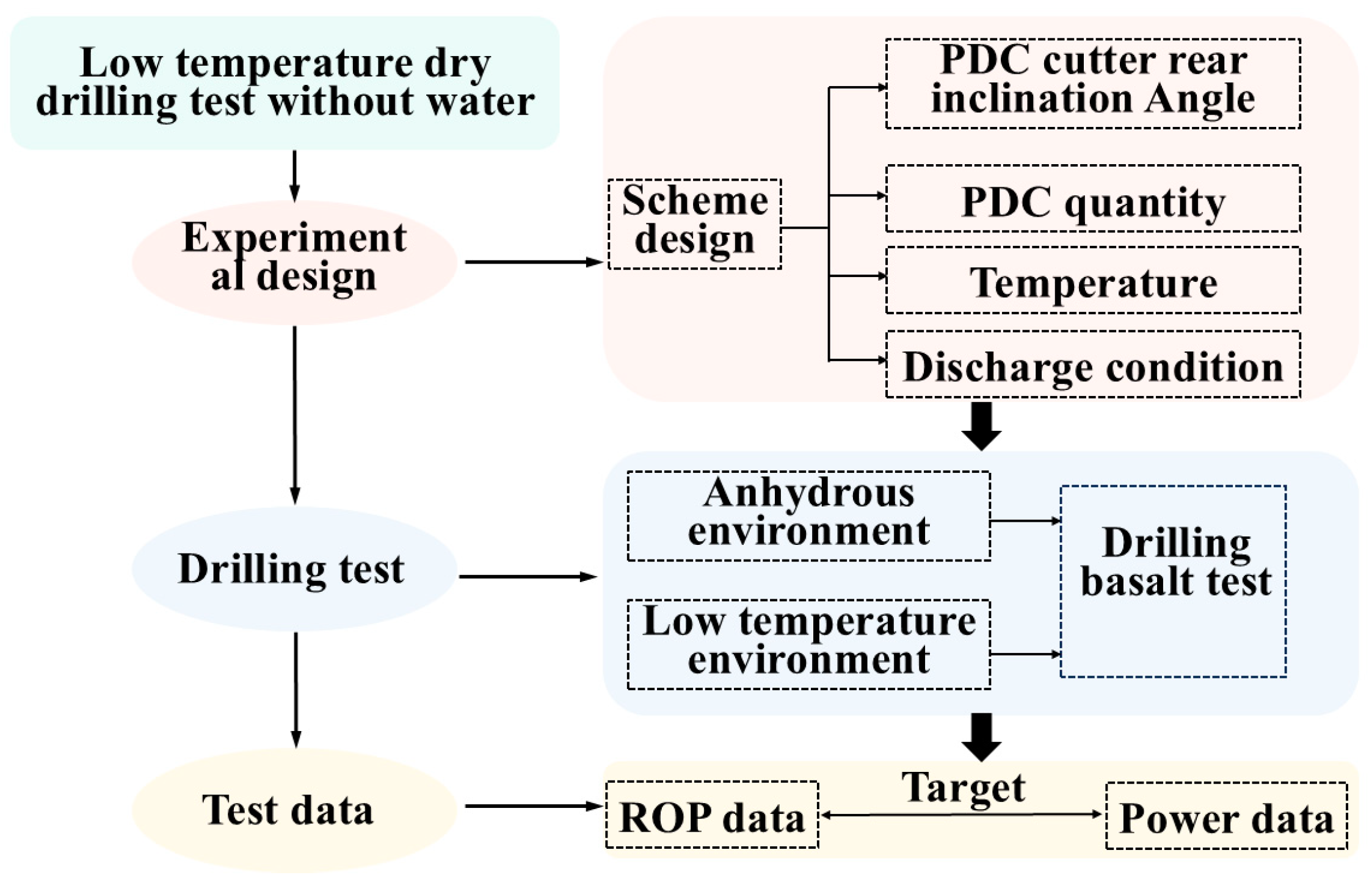
This low-temperature, anhydrous dry drilling test is designed to simulate the unique conditions of the lunar surface. The test program aims to perform drilling operations while measuring the key parameters, including the ROP and power consumption. The specific process is illustrated in Figure 1.

After evaluating and comparing various types of drilling bits, the PDC bit was found to be the most suitable for deep lunar drilling due to its high drilling efficiency and moderate power consumption [26,27]. In this experiment, the PDC bit was selected as the drilling tool. A four-factor, three-level RSM experiment was designed, focusing on the number of cutting teeth, backward inclination angle (the angle between the cutting face and the outer normal of the rock face at the bottom of the hole), temperature, and chip removal conditions. It was found that the temperature near the lunar equator is approximately −30 °C, and the temperature variations in the lower layers of the lunar surface remain relatively constant [28]. The test temperatures were set at −55 °C, −35 °C, and −15 °C. Drilling was conducted under waterless conditions, with rock dust being removed by a low-power exhaust fan (an exhaust fan with a rated power of only 35 W), which is considered the chip removal condition. The chip removal conditions were categorized into three levels, corresponding to the gear positions of the exhaust fan: level 1 for the lowest gear, level 2 for the mid-range gear, and level 3 for the highest gear, providing the most effective debris removal. The PDC cutting tools were arranged in three configurations: two, three, and four cutting teeth, based on conventional cutting tooth arrangements. The backward inclination angle of the PDC cutting teeth typically ranges from 5° to 25°, with the angles for this experiment set at 5°, 15°, and 25°. The waterless dry drilling test program is shown in

Table 1. Low-temperature anhydrous dry drilling test design program.

Factors Influencing the Experiment	Factor Level Value
Temperature (°C)	−55	−35	−15
Debris removal conditions	1	2	3
The number of PDC cutting teeth (z)	2	3	4
PDC cutting teeth backward angle (°)	5	15	25

. By integrating the dry drilling test design with response surface methodology, a total of 29 sets of physical tests were conducted.

2.2. Simulation of the Lunar Surface Environment

The Moon’s anhydrous environment and extreme temperature variations differ significantly from those on Earth. Therefore, when designing drilling tests, it is crucial to simulate these unique environmental conditions as accurately as possible. The simulations primarily aimed to replicate the anhydrous environment and low-temperature conditions.

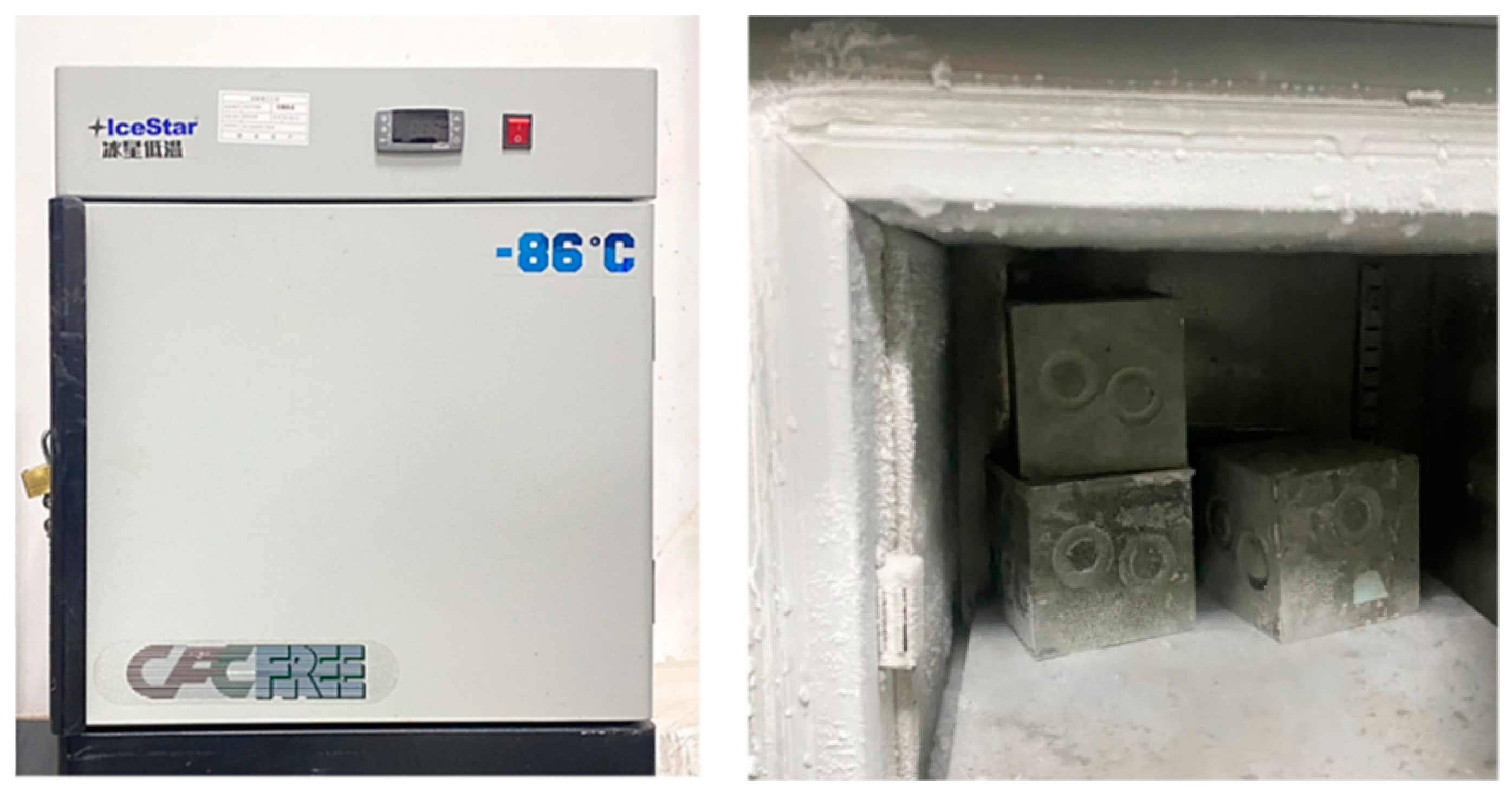
The cryogenic environment was simulated by placing basalt samples in a specialized freezer unit designed specifically for the dry drilling test. This unit was capable of reaching a low temperature of −86 °C, effectively cooling the samples for the experiment. 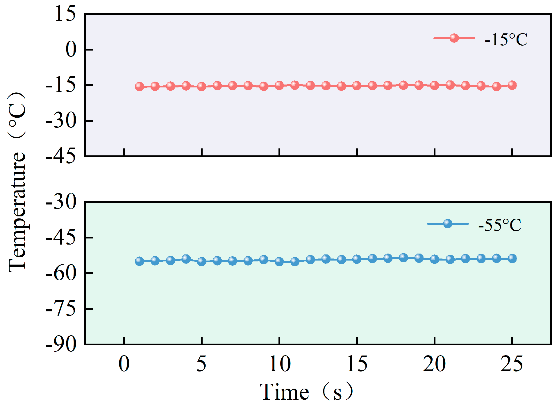After placing the samples in the freezer, the temperature was adjusted to the target value, and both the test setup and the samples were frozen, as shown in Figure 2. To mitigate the impact of indoor temperature fluctuations on the test results, a control test was conducted in a room-temperature environment. In this test, the rock samples were first frozen at −55 °C and −15 °C. After freezing, the samples were removed from the freezer and placed in the room-temperature environment, where their temperature changes were measured. Figure 3 shows that the temperature changes were nearly linear, indicating that environmental factors did not influence the temperature during the test, allowing it to remain stable at the designed value.

The lunar surface has limited water resources, meaning that transporting flushing media and the necessary devices for drilling would not only increase the probe’s energy consumption, but also complicate the drilling process. Therefore, conducting exploration in the deeper regions of the Moon without using a flushing medium is more practical. In this study, the rock samples were drilled using a dry drilling method, with a low-power exhaust fan employed to maintain a water-free environment. During the drilling tests, the exhaust fan was positioned at the drilling site, and its speed was adjusted according to the test parameters. This setup enabled the efficient removal of rock dust generated during drilling.

2.3. Test Materials

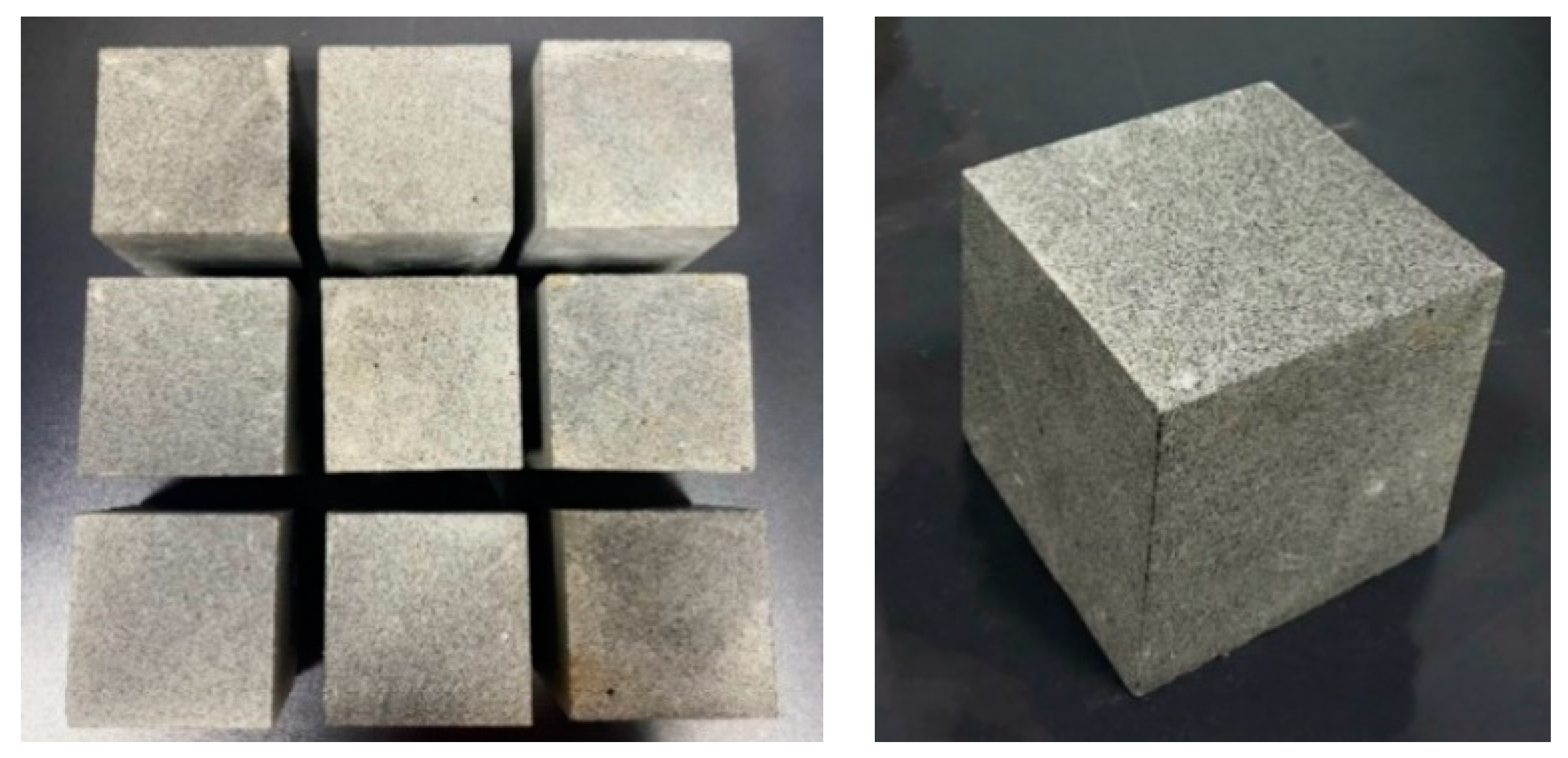
Research indicates a significant presence of lunar mare basalt based on the analysis of lunar rock samples and lunar surface exploration [29,30]. Basalt was chosen as the rock sample for this low-temperature, anhydrous drilling test. To meet the size requirements of the drilling equipment, the basalt was shaped into a square sample with dimensions of 100 mm in length, width, and height, as shown in Figure 4.

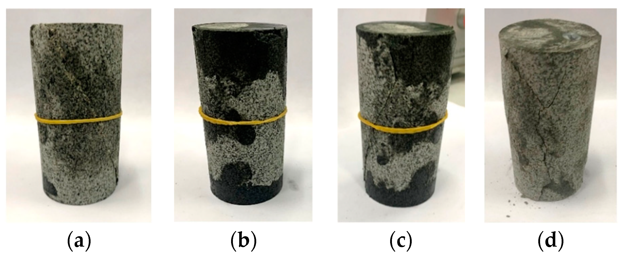
To fully demonstrate basalt’s ability to resist damage from external forces and its rock properties under load, before the drilling test, a preliminary mechanical assessment was conducted, yielding a uniaxial compressive strength of 93.6 MPa and a tensile strength of 15.23 MPa, indicating that basalt is a very hard rock. To further investigate its behavior under complex stress conditions, a triaxial test was performed. This test allowed for the measurement of the relevant physical and mechanical properties of basalt and the determination of the mechanical parameters at various damage levels, as shown in

Table 2. The physical and mechanical properties of basalt.

Confining Pressure (MPa)	Compressive Strength (MPa)	Tensile Strength (MPa)	Shearing Strength (MPa)	Elastic Modulus (10 GPa)
2	100.5	25.5	50.1	7.17
4	102.1	24.3	53.7	5.28
6	115.5	31.2	53.9	6.28
8	114.1	27.5	59.8	5.96

. The damaged rock samples following the mechanical tests are shown in Figure 5.

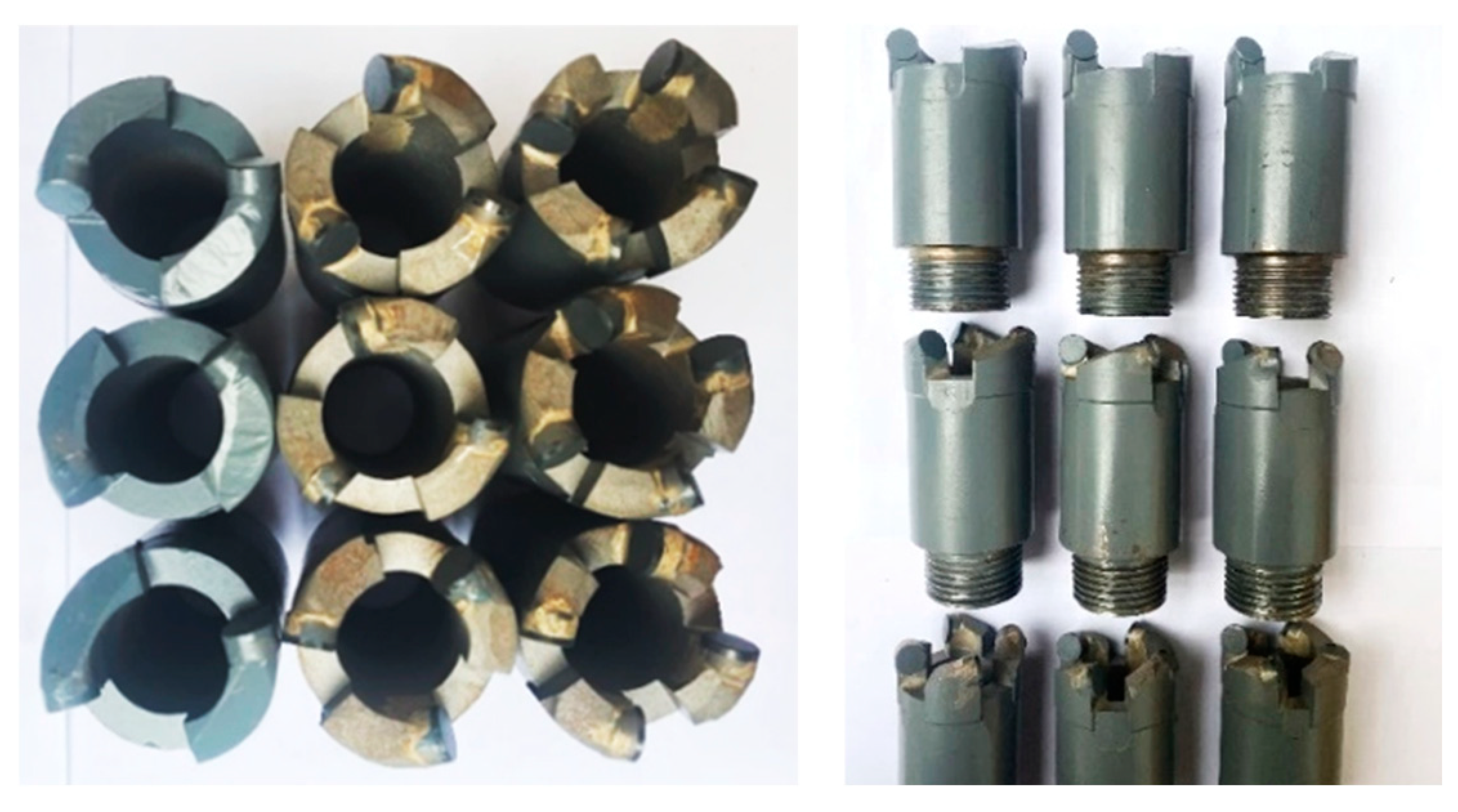
The specifications of the drill body were as follows: an inner diameter of 21.1 mm, an outer diameter of 35 mm, and a height of 85 mm, with one edge having a width of 0.6 mm. The cutting tool selected was a standard round PDC composite piece, with a diameter of 8 mm and a thickness of 1 mm. According to the test program, nine types of PDC cutting tools were developed, each featuring varying numbers of cutting teeth and different negative front angles. The configurations included designs with two cutting teeth at negative front angles of −5°, −15°, and −25°; three cutting teeth at the same angles; and four cutting teeth at −5°, −15°, and −25°. Based on this analysis, nine physical drawings of the PDC drills were created and machined specifically for the dry drilling tests, as shown in Figure 6.

2.4. Experimental Testing Device

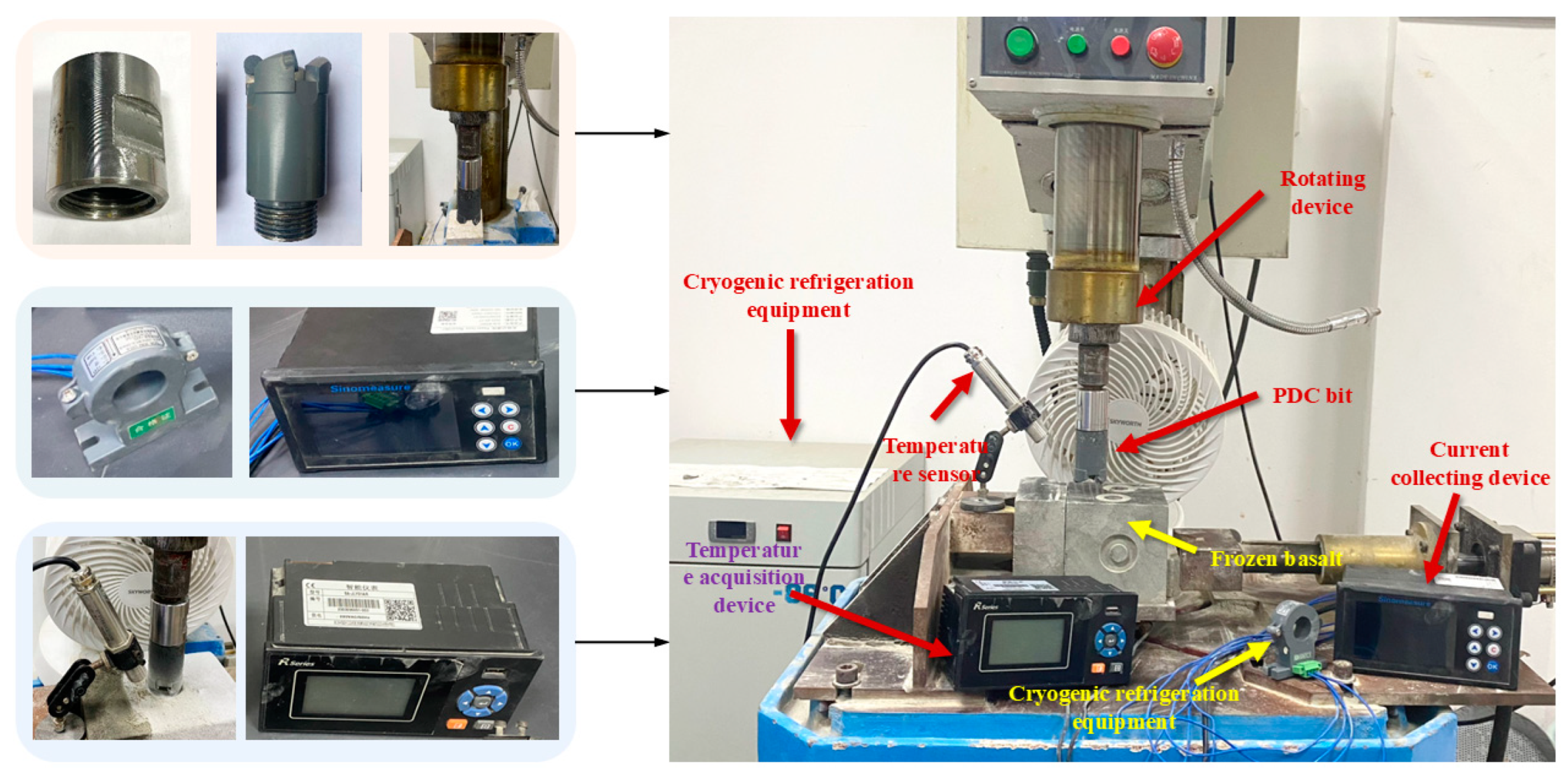
The dry drilling test was conducted using a ZK5040BS/2 micro drilling rig (Zhejiang Aimake Machine Tool Co., Ltd., Wenzhou, China), which features a high-strength, gear-driven main transmission system and a numerical control system for managing the feed mechanism. The core unit of the test includes a rotary feeding device, a drilling rig, a connecting device, and a monitoring system that collects current and temperature data during the drilling process. The test setup and operating platform are shown in Figure 7. The key parameters of the device are provided in

Table 3. Key parameters of test device.

Parameter Name	Parameter Value
Range of rotational speed	67~1780 r/min
Number of steps of rotational speed	12
Feed speed	0~5000 mm/min
Rated power	2.8 KW
Maximum drilling diameter	40 mm

. The temperature of the frozen rock sample was measured by the temperature sensor in Figure 7.

3. Modeling and Analysis of ROP Response Surface

3.1. Experimental Data

The physical testing of the basalt drilling was conducted under low-temperature and dry conditions, as per the test program. The ROP and current data were measured, and the power was calculated from the current using the formula shown in Equation (1),

$$P=UI$$

(1)

where P is the power consumed during drilling, U is the rated voltage, and I is the current of drilling.

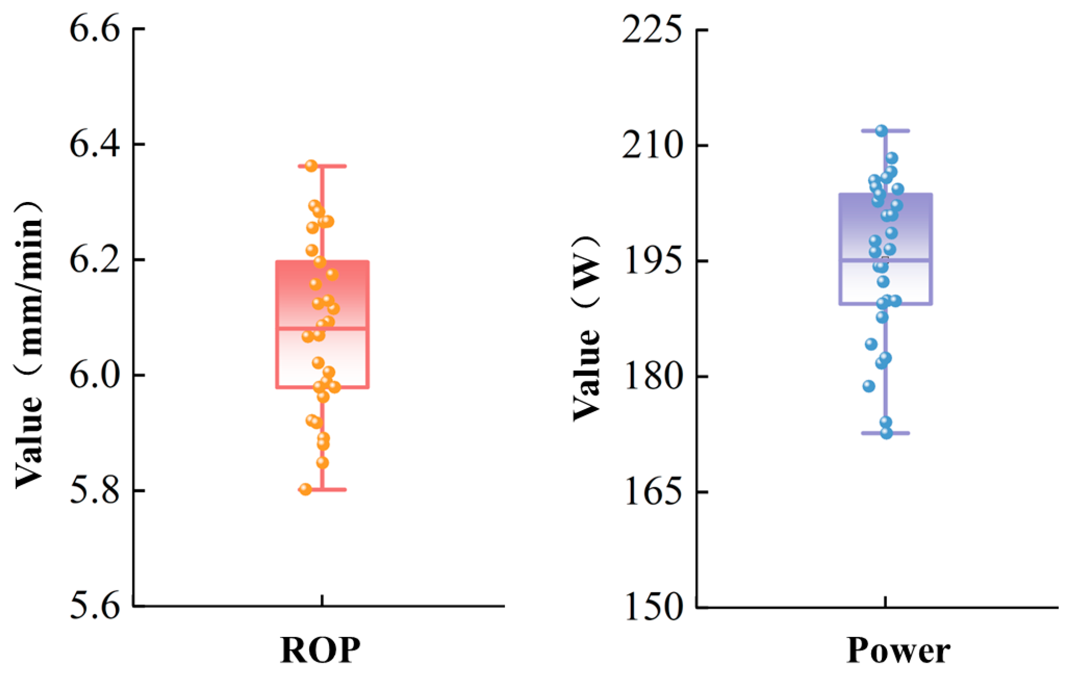
The rated voltage of the drilling equipment used in the test was 380 V. The power consumption was calculated using Equation (1). Due to the minimal wear on the drill bit after three drilling tests, the ROP and power data from the final dry drilling test were averaged using a weighted ratio of 3:3:4, as shown in

Table 4. Waterless dry drilling test measured data.

No.	Negative Anterior Angle (°)	PDC Cutting Teeth (z)	Temperature (°C)	Chip Removal Conditions	ROP (mm/min)	Power (W)
1	15	4	−35	3	6.22	196.16
2	25	3	−55	2	6.12	181.73
3	15	2	−55	2	6.29	202.72
4	5	3	−35	1	6.12	202.18
5	25	4	−35	2	6.07	184.18
6	15	4	−15	2	6.27	189.85
7	15	4	−35	1	6.20	192.29
8	15	3	−55	3	6.36	205.42
9	25	3	−35	1	5.85	174.07
10	15	3	−55	1	6.13	198.60
11	15	3	−35	2	5.92	197.57
12	25	2	−35	2	5.80	178.74
13	15	2	−35	1	5.99	196.47
14	5	3	−35	3	6.09	208.35
15	5	4	−35	2	6.16	194.28
16	25	3	−35	3	6.09	182.40
17	15	3	−35	2	5.89	200.84
18	25	3	−15	2	5.88	172.64
19	15	2	−35	3	6.27	206.54
20	5	2	−35	2	6.02	211.89
21	15	4	−55	2	6.28	187.67
22	15	3	−35	2	5.96	205.76
23	5	3	−55	2	6.01	200.95
24	15	3	−35	2	5.98	204.32
25	15	2	−15	2	5.98	189.45
26	5	3	−15	2	6.26	204.55
27	15	3	−15	3	6.07	194.22
28	15	3	−35	2	5.92	203.61
29	15	3	−15	1	6.17	189.80

. Based on the test data, Figure 8 shows that the ROP values are concentrated between 5.8 and 6.4 mm/min, with an average ROP of 6.08 mm/min. The power data range from 165 to 225 W, with an average of 195.08 W.

3.2. The Regression Model of ROP Was Established

RSM is a mathematical approach used to model the relationship between the experimental design and the resulting data [31,32]. This study investigates the nonlinear relationship between response values and influencing factors using an established regression-fitting model. RSM is applied in this paper to develop a predictive equation that links the target parameters to the influencing factors.

Based on the test results, the test factors are defined as follows: the PDC backward inclination angle (N₁), the number of PDC teeth (N₂), the temperature (N₃), and the chip removal condition (N₄). The ROP is the response variable (M₁), and the nonlinear regression model for ROP is presented in Equation (2).

$$\begin{array}{l}{M}_1=5.93-0.0699N_1+0.0696N_2-0.0477N_3+0.0535N_4\\ +0.0321N_1{N}_2-0.1237N_1{N}_3+0.0652N_1{N}_4+0.0740N_2{N}_3\\ -0.0646N_2{N}_4-0.0847N_3{N}_4-0.0220{N_1}^2+0.1133{N_2}^2\\ +0.1490{N_3}^2+0.1144{N_4}^2\end{array}$$

(2)

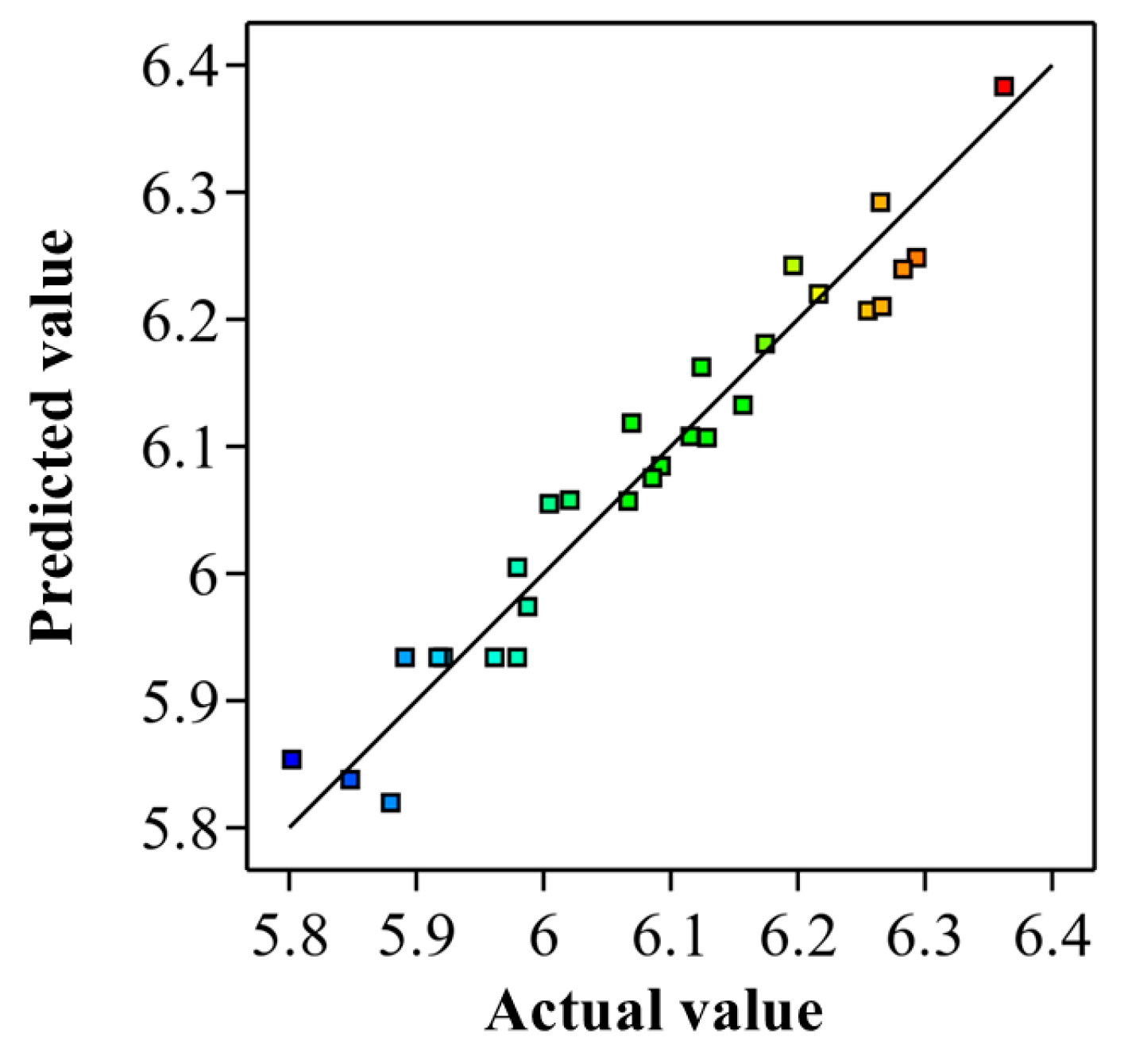
To assess the accuracy of the regression model, the predicted ROP values were compared with the actual observed values.

Table 5. ROP predicted vs. actual value.

No.	Actual Value	Predicted Value	No.	Actual Value	Predicted Value	No.	Actual Value	Predicted Value
1	6.22	6.22	11	5.92	5.93	21	6.28	6.24
2	6.12	6.16	12	5.80	5.85	22	5.96	5.93
3	6.29	6.25	13	5.99	5.97	23	6.01	6.06
4	6.12	6.11	14	6.09	6.08	24	5.98	5.93
5	6.07	6.06	15	6.16	6.13	25	5.98	6.00
6	6.27	6.29	16	6.09	6.08	26	6.26	6.21
7	6.20	6.24	17	5.89	5.93	27	6.07	6.12
8	6.36	6.38	18	5.88	5.82	28	5.92	5.93
9	5.85	5.84	19	6.27	6.21	29	6.17	6.18
10	6.13	6.11	20	6.02	6.06

presents the predicted and actual values, while the comparison results are shown in Figure 9. The comparison reveals that the actual values closely align with the predicted values, demonstrating the model’s high accuracy.

3.3. Analysis of Variance (ANOVA)

Response surface modeling focuses on investigating the functional relationship between the test factors and the response, emphasizing significance, analysis of variance, and confidence testing. According to the variance results presented in

Table 6. Analysis of variance (ANOVA) for ROP modeling.

Project	Sum of Squares	Degrees of Freedom	Mean Square	F	p
Model	0.5951	14	0.0425	17.42	<0.0001
N1	0.0586	1	0.0586	24.00	0.0002
N2	0.0581	1	0.0581	23.80	0.0002
N3	0.0273	1	0.0273	11.20	0.0048
N4	0.0343	1	0.0343	14.05	0.0022
N1N2	0.0041	1	0.0041	1.69	0.2145
N1N3	0.0612	1	0.0612	25.07	0.0002
N1N4	0.0170	1	0.0170	6.96	0.0195
N2N3	0.0219	1	0.0219	8.98	0.0096
N2N4	0.0167	1	0.0167	6.85	0.0203
N3N4	0.0287	1	0.0287	11.75	0.0041
N12	0.0031	1	0.0031	1.28	0.2765
N22	0.0832	1	0.0832	34.10	<0.0001
N32	0.1439	1	0.1439	58.96	<0.0001
N42	0.0849	1	0.0849	34.77	<0.0001
Residual	0.0342	14	0.0024
Misfit term	0.0291	10	0.0029	2.28	0.2221
Pure error	0.0051	4	0.0013
Total error	0.6293	28

and the significance evaluation index in

Table 7. Significance evaluation index.

p-Value	p < 0.001	0.001 < p < 0.05	p > 0.05
Significance	Highly significant	Significant	Insignificant

, the p-value for the coefficients in the regression model is less than 0.0001 (p < 0.0001), indicating that the model is highly significant and valuable for research. The p-value for the dislocation term is 0.2221, which exceeds 0.05, suggesting that the dislocation term is not significant and that no dislocation factor exists in the model.

Additionally, Table 6 shows that the p-values for N₁, N_2, and the interaction term N₁ N₃ are all below 0.001, indicating that the effects of these factors on the ROP are highly significant. The p-values for N₃, N₄, N₁ N₄, N₂ N₃, N₂ N₄, and N₃ N₄ range from 0.001 to 0.05, indicating that these factors also have a significant effect on the ROP. In contrast, the p-value for N₁N₂ exceeds 0.05, indicating that its effect is not significant.

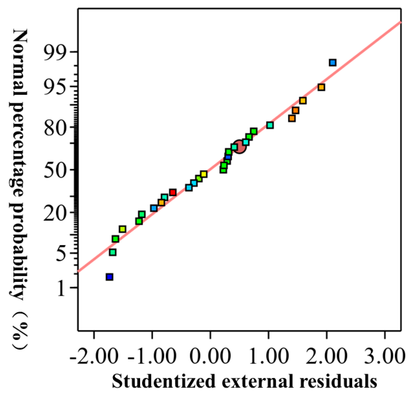
The confidence analysis in

Table 8. Confidence testing of ROP model.

C.V.%	R2	Adjusted R2 (Rpre2)	Predicted R2 (Rpre2)	Adeq Precision
0.8125	0.9457	0.8914	0.7213	15.8594

shows that the precision of the ROP model is 15.8594 (>4), and the coefficient of variation (C.V.) is 0.8125% (<10%), indicating that the model exhibits good reliability. The coefficient of determination (R²) is 0.9457; it represents the degree of agreement between the model’s predicted values and the actual data, where a higher R² value closer to one indicates a better model fit. The difference between it and the adjusted R² (R_Adj²) is 0.0543, which suggests a strong correlation between the independent terms of the model. Furthermore, based on the Student’s quantification of the outer residuals in Figure 10, no outliers are present, and the residuals are nearly aligned along a straight line. This indicates that the model has a good fit and can be effectively used in response surface experiment design.

3.4. Response Surface of ROP

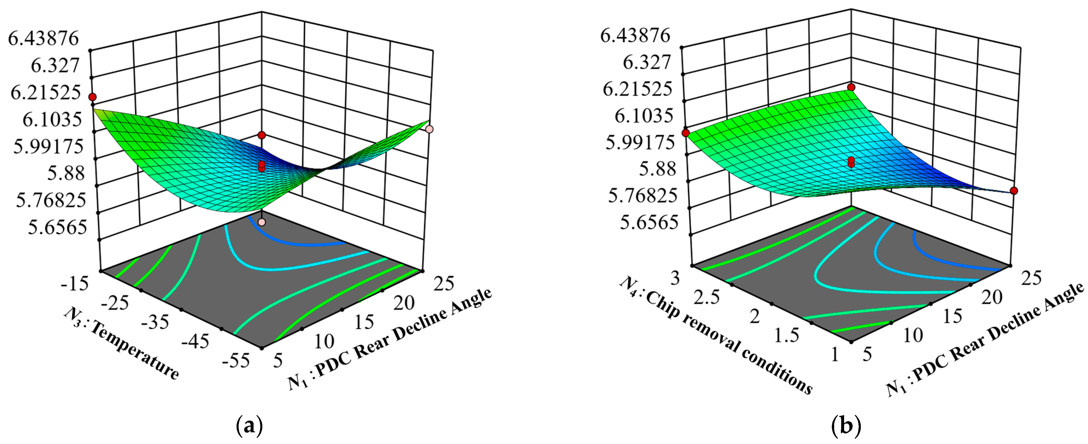
To investigate the impact of the number of PDC teeth, backward inclination angle, temperature, and chip removal conditions on the ROP, the nonlinear regression equation from Equation (2) was used to calculate the three-dimensional response surface (a surface of the relationship between one dependent variable and multiple independent variables), illustrating the relationship between the ROP and the aforementioned factors. This surface is presented in Figure 11, where the figure represents the corresponding surface of the interaction effects of the experimental factors on the ROP. In response surfaces, a steeper inclination indicates that the interaction between the two test influencing factors has a more significant effect on the ROP, while a flatter surface suggests a weaker interaction.

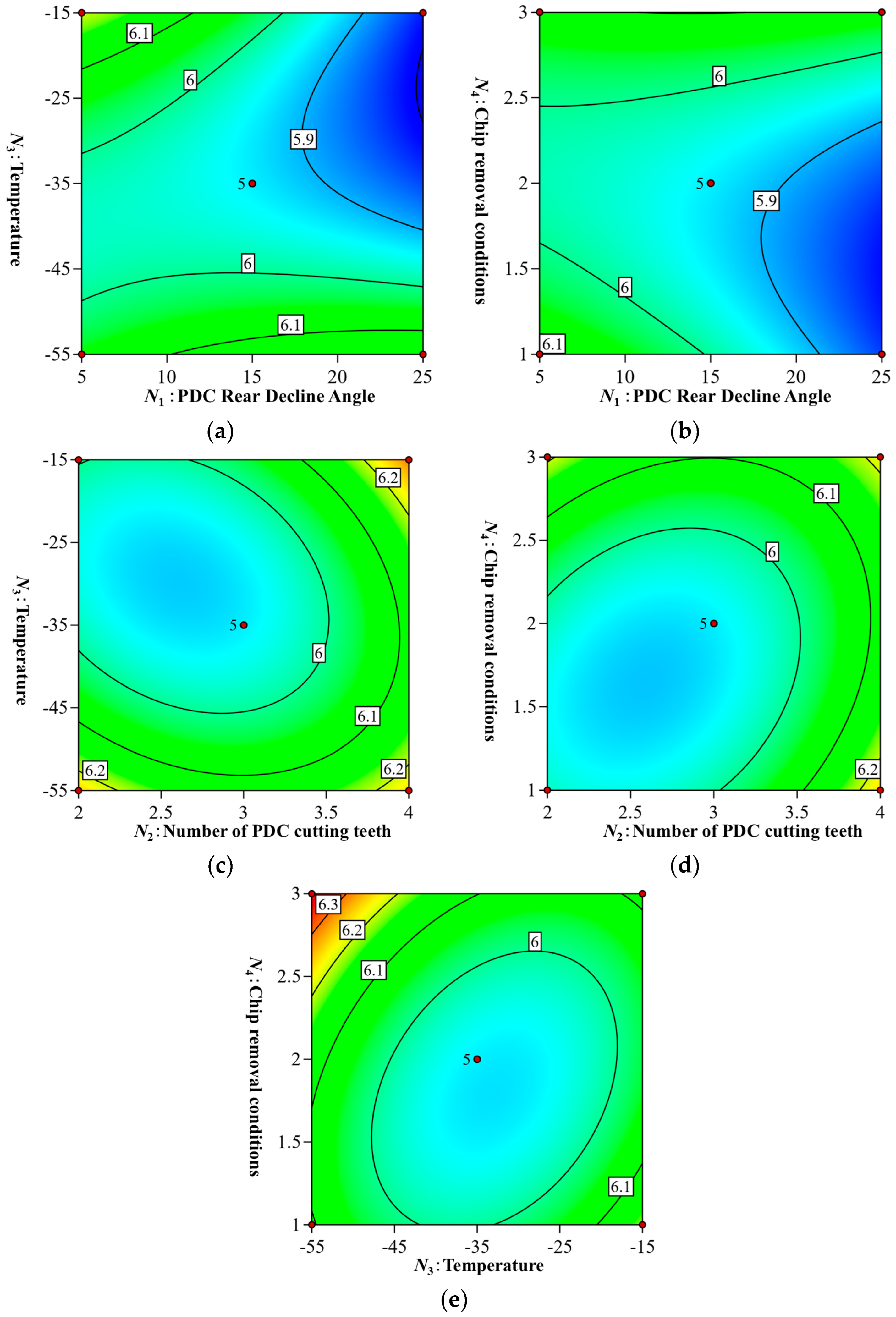
Figure 12 shows the contour plot of the response surface from Figure 11 projected onto the bottom. The combination of response surfaces and contours provides a more intuitive means of analyzing the model. As shown in Figure 11a and Figure 12a, the ROP increases from 6.005 mm/min to 6.124 mm/min (a 2% increase) as the backward inclination angle rises from 5° to 25° at −55 °C. At −15 °C, however, the ROP decreases from 6.255 mm/min to 5.88 mm/min (a 6% decrease) as the backward inclination increases from 5° to 25°. This suggests that, at lower temperatures, increasing the backward inclination angle has little effect on the ROP, while at higher temperatures, a larger angle leads to a significant decrease in the ROP, thereby reducing drilling efficiency.

The steep slope of the response surface in Figure 11b, combined with the elliptical contour in Figure 12b, indicates a significant interaction between N₁ and N₄, affecting the ROP. As the chip removal condition increases, the ROP remains constant with an increasing backward inclination angle. However, when the chip removal condition is at its lowest level (Level 1), increasing the backward inclination angle from 5° to 25° causes a decrease in the ROP from 6.115 mm/min to 5.848 mm/min. Under minimal chip removal conditions and in the absence of a flushing medium, rock chips cannot be efficiently evacuated from the hole, leading to their accumulation. If not promptly cleared, this buildup increases the load on the drill bit, potentially leading to bit blockage, accelerated wear, and reduced drilling efficiency. Even with an increase in the backward inclination angle, the effect is only the repeated crushing of rock powder, which does not improve the ROP.

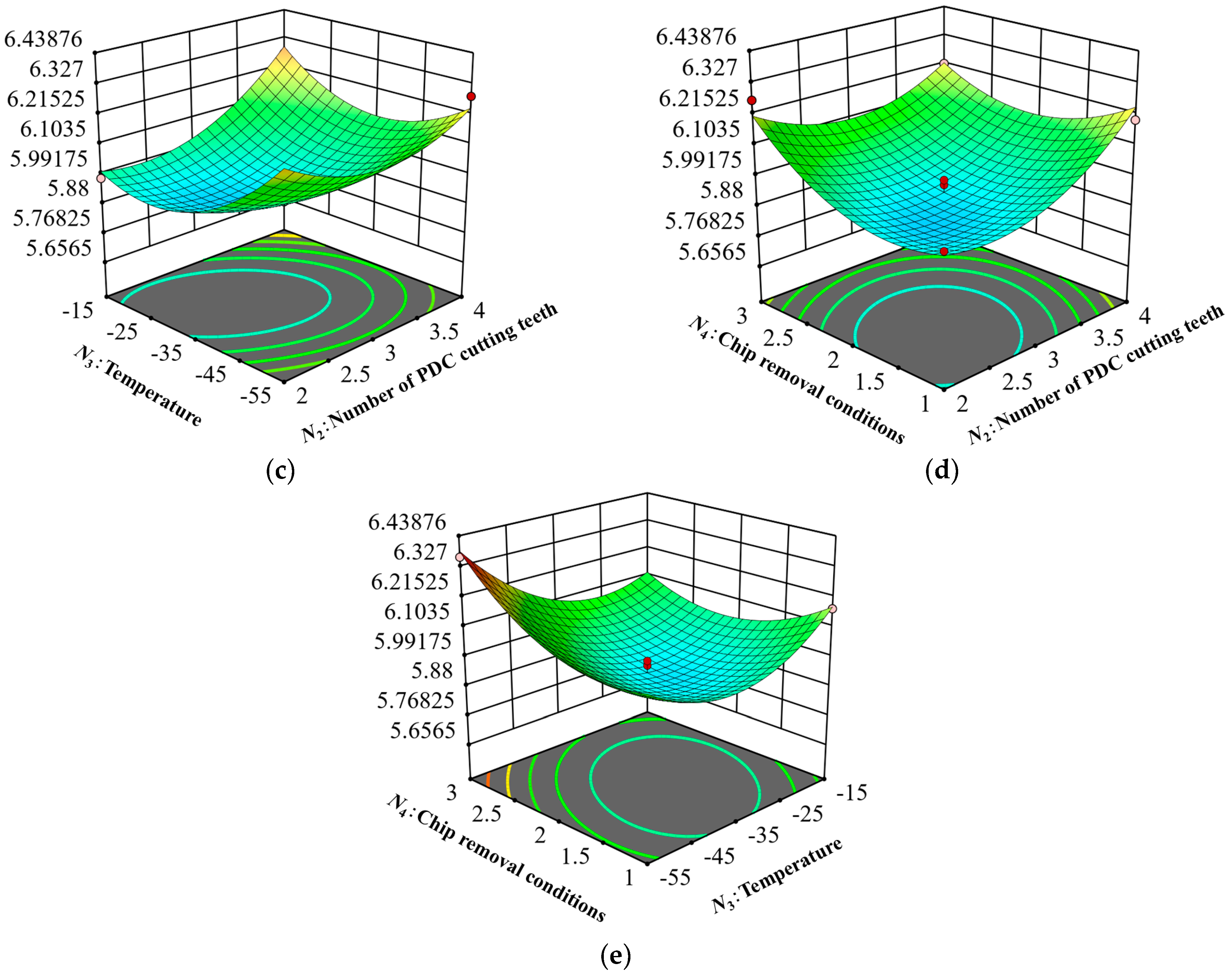
Figure 11c presents a parabolic response surface with an upward-facing opening, and the corresponding contour plot in Figure 12c is elliptical. This indicates that the interaction between the number of cutting teeth and the temperature significantly affects the ROP, with a minimum response observed under these conditions. The number of cutting teeth ranges from two to four, and the temperature ranges from −25 °C to −45 °C, during which the ROP remains low, at only 5.89 mm/min.

The response surface shown in Figure 11d and the contour in Figure 12d reveal that the ROP reaches its lowest values when the number of cutting teeth is between 2.5 and 3.5, and when the chip removal condition is between 1.5 and 2.5. With a fixed number of cutting teeth, the ROP increases as chip removal conditions improve. This suggests that enhancing the chip discharge facilitates the removal of rock dust generated during drilling, reducing the accumulation and repeated crushing of debris, and thus improving drilling efficiency.

Combining Figure 11e and Figure 12e, we observe that at temperatures between −25 °C and −45 °C and chip removal conditions between 1.5 and 2.5, the ROP remains at its lowest. At higher temperatures, the change in ROP tends to be gentle with the increase in chip removal conditions. Conversely, at lower temperatures, the ROP increases with the increase in chip removal conditions. The color gradient in the response surface indicates a rapid shift in ROP from low to high. Specifically, at a temperature of −55 °C and with the chip removal conditions increasing from 1 to 3, the ROP increases from 6.13 mm/min to 6.36 mm/min.

4. Power Response Surface Modeling and Analysis

4.1. Modeling

Using the same establishment method as the ROP regression model in Section 3.2, a nonlinear regression model is established with power as the response variable (M₂). This model relates the four influencing factors to the response variables, as shown in Equation (3). Based on the coefficients of N₁, N₂, N₃, and N₄ in Equation (3), the strongest relationship is observed between M₂ and N₁. This relationship aligns with the effect of the cutting teeth inclination angle on the power consumption in conventional drilling tests.

$$\begin{array}{l}{M}_2=202.42-12.37N_1-3.45N_2-3.05N_3+3.31N_4\\ +5.76N_1{N}_2-3.18N_1{N}_3+0.54N_1{N}_4+3.86N_2{N}_3\\ -1.55N_2{N}_4-0.6006N_3{N}_4-7.76{N_1}^2-3.48{N_2}^2\\ -5.06{N_3}^2+1.45{N_4}^2\end{array}$$

(3)

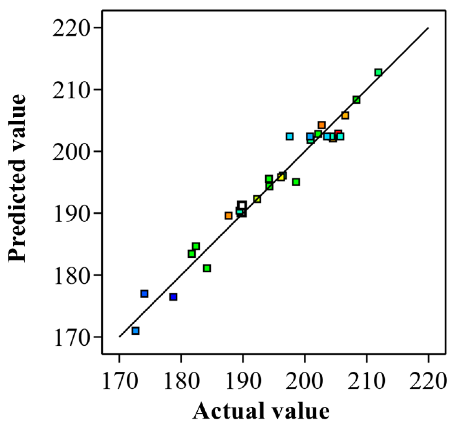
To verify the accuracy of the power regression model, the predicted values were obtained from the regression equation, as shown in the

Table 9. Power prediction vs. actual value.

Number	Actual Value	Predicted Value	Number	Actual Value	Predicted Value	Number	Actual Value	Predicted Value
1	196.16	195.81	11	197.57	202.42	21	187.67	189.62
2	181.73	183.45	12	178.74	176.49	22	205.76	202.42
3	202.72	204.24	13	196.47	196.09	23	200.95	201.84
4	202.18	202.81	14	208.35	208.35	24	204.32	204.42
5	184.18	181.12	15	194.28	194.34	25	189.45	190.42
6	189.85	191.25	16	182.40	184.68	26	204.55	202.10
7	192.29	192.29	17	200.84	202.42	27	194.22	195.57
8	205.42	202.87	18	172.64	171.00	28	203.61	202.42
9	174.07	177.00	19	206.54	205.80	29	189.80	190.16
10	198.60	195.05	20	211.89	212.76

, and compared with the actual power values. The comparison reveals a close alignment between the predicted and actual values, confirming the high accuracy of the model, as illustrated in Figure 13.

4.2. Analysis of Variance

To assess the variations among different test groups and evaluate the effects of the various test factors on the power results, significance, ANOVA, and confidence tests were conducted on the power model. The calculated results are presented in

Table 10. Analysis of variance for power modeling.

Project	Sum of Squares	Degrees of Freedom	Mean Square	F	p
Model	2963.71	14	211.69	25.78	<0.0001
N1	1836.75	1	1836.75	223.71	<0.0001
N2	142.63	1	142.63	17.37	0.0009
N3	111.51	1	111.51	13.58	0.0024
N4	131.26	1	131.26	15.99	0.0013
N1N2	132.90	1	132.90	16.19	0.0013
N1N3	40.32	1	40.32	4.91	0.0438
N1N4	1.17	1	1.17	0.1421	0.7119
N2N3	59.73	1	59.73	7.28	0.0174
N2N4	9.59	1	9.59	1.17	0.2981
N3N4	1.44	1	1.44	0.1757	0.6814
N12	390.97	1	390.97	47.62	<0.0001
N22	78.44	1	78.44	9.55	0.0080
N32	166.14	1	166.14	20.24	0.0005
N42	13.60	1	13.60	1.66	0.2189
Residual	114.95	14	8.21
Misfit term	72.71	10	7.27	0.6885	0.7127
Pure error	42.24	4	10.56
Total error	3078.66	28

and

Table 11. The confidence testing of the power model.

C.V.%	R2	Adjusted R2 (RAdj2)	Predicted R2 (Rpre2)	Adeq Precision
1.47	0.96	0.93	0.84	20.27

. Based on the significance evaluation indices in Table 7, the p-value for the regression term of the power model is less than 0.0001, indicating that the model is highly significant. The p-value for the misfit term is 0.7241, which is greater than 0.05, indicating that the misfit term is not significant and that the power model can be used to analyze the effects of the four test factors on the power.

From the ANOVA table of the power model, it can be observed that the p-value for N₁ is less than 0.001, indicating high significance. The p-values for N₂, N₃, N₄, N₁ N₂, and N₁ N₃, as well as N₂ N₃, range from 0.001 to 0.05, indicating statistical significance. However, the p-values for N₁ N₄, N₂ N_4, and N₃ N₄ are all greater than 0.05, which means non-significance.

Additionally, as shown in Table 11, the coefficient of determination (R²) for the power model is 0.96, demonstrating a strong correlation and high model credibility.

4.3. Response Surface of Power

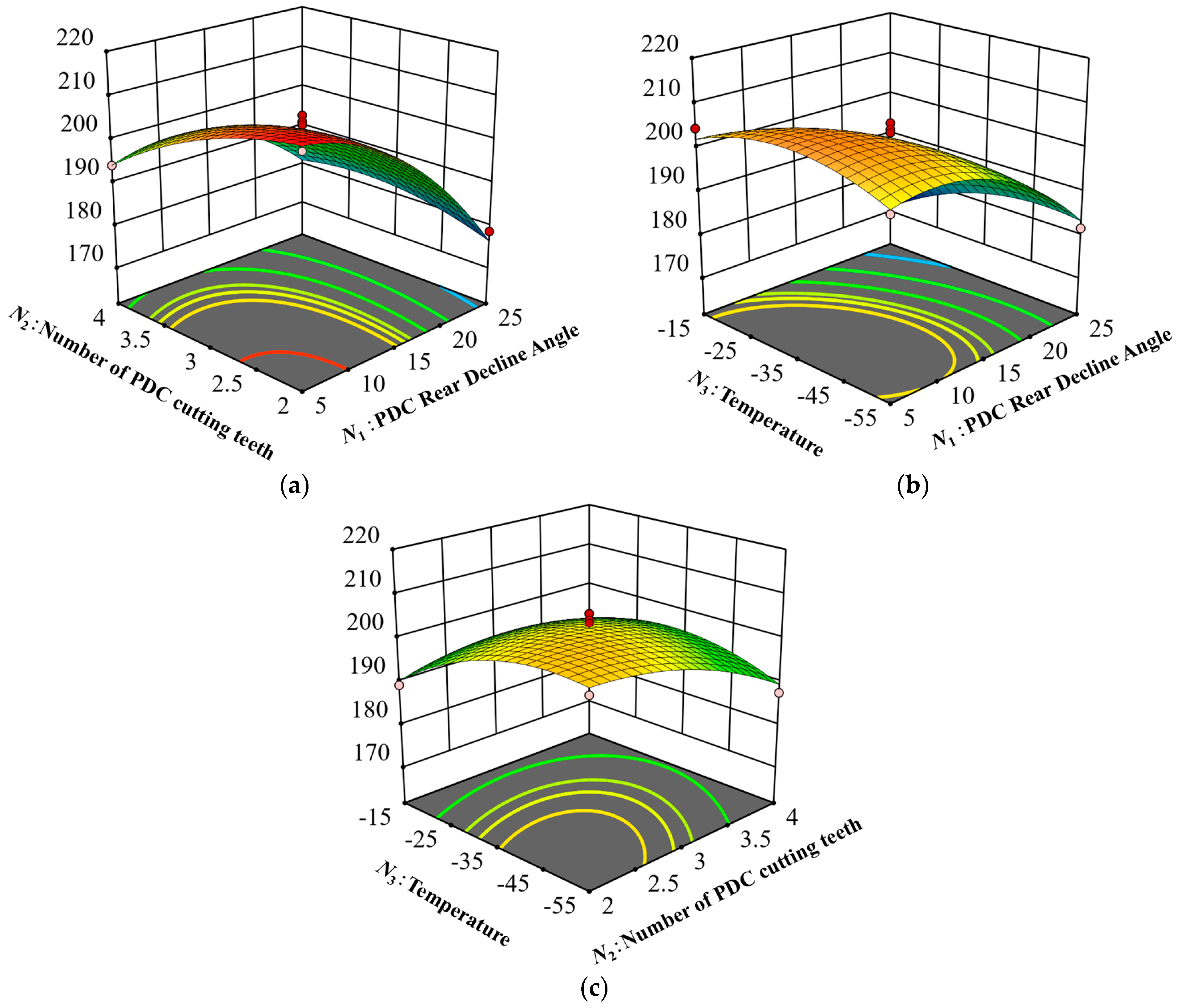
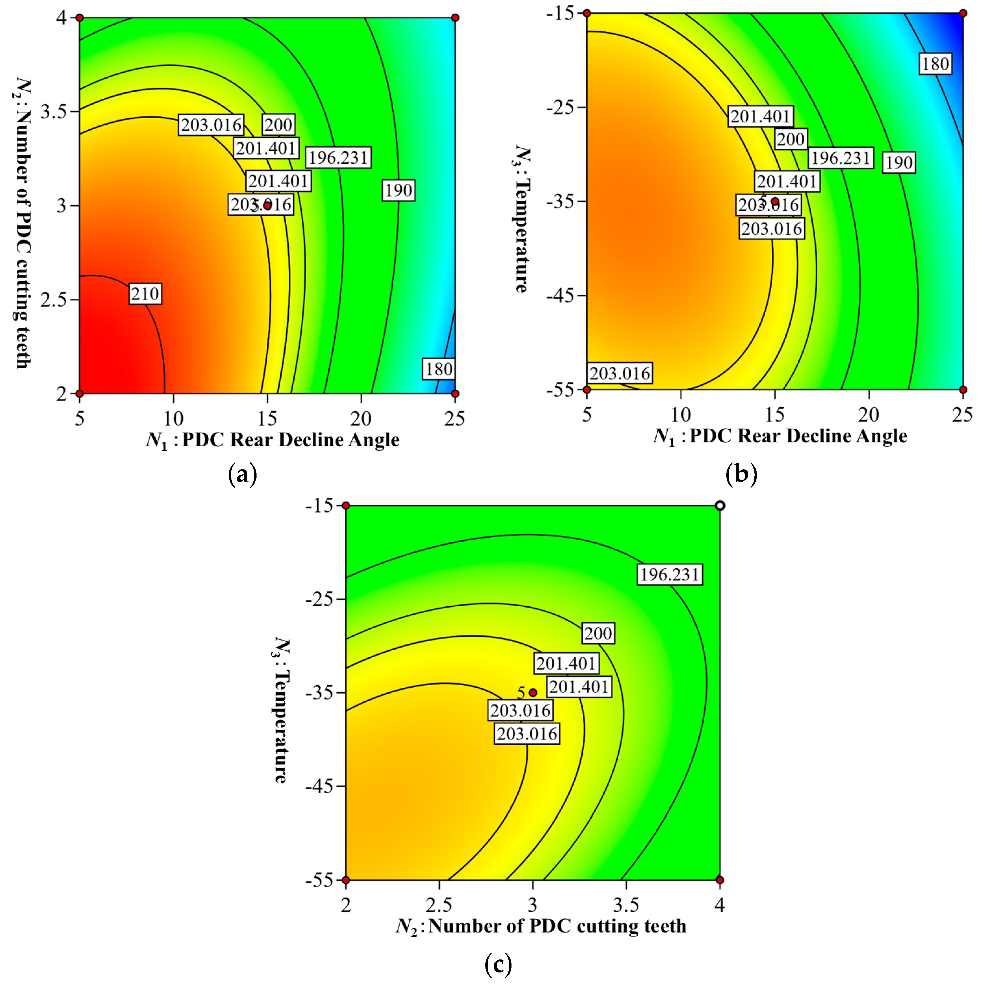
Based on the nonlinear regression equation established by Equation (3), a three-dimensional response surface was calculated to analyze the effects of the interactions between the power and the number of PDC teeth, backward inclination angle, temperature, and chip removal conditions. A comprehensive evaluation was then conducted by examining the response surface in Figure 14 in conjunction with the contour lines in Figure 15.

The slope of the response surface in Figure 14a is steep, and the color transition from blue to red indicates a rapid increase in power, suggesting that the interaction between the factors has a significant effect on power. The contours in Figure 15a are elliptical, highlighting the significant interaction between N₁ and N₂ on power. The power consumption decreases from 194.28 W to 184.18 W when the number of cutting teeth is four and the backward inclination angle increases from 5° to 25°. With two cutting teeth and an increase in the backward inclination angle from 5° to 25°, the power consumption decreases notably, from 211.89 W to 178.74 W, representing a reduction of 15.6%. This reduction can be attributed to the fact that a smaller angle results in an unstable drilling process, causing significant vibration and increased power consumption, while a larger angle helps stabilize the drilling process, thereby reducing the power consumption.

Figure 14b shows that the downward-opening response curve with a curved slope indicates a significant interaction between N₁ and N₃ that affects power. The elliptical contours in Figure 15b further support the considerable influence of this interaction on power. At a given temperature, the power consumption decreased markedly as the backward inclination angle increased. Specifically, at −55 °C, the power consumption during the drilling process decreased from 200.95 W to 181.73 W when the backward inclination angle was increased from 5° to 25°, representing a 9.6% reduction. At higher temperatures, the effect of increasing the rear camber on power becomes more pronounced. At −15 °C, increasing the rear camber from 5° to 25° reduced the power consumption from 204.55 W to 172.64 W, a significant decrease of 15.6%.

Figure 14c displays a parabolic response surface plot with a downward-facing opening, showing a trend of power initially increasing and then decreasing, which suggests the presence of extreme values in the response surface. In Figure 15c, the elliptical contours representing the interaction between the temperature and the number of PDC cutting teeth further emphasize the significant effect of this interaction on power. At higher temperatures, power consumption remains largely unaffected by changes in the number of PDC cutting teeth. However, at lower temperatures, power tends to decrease as the number of cutting teeth increases. Specifically, at −55 °C, increasing the number of PDC cutting teeth from two to four reduces the power consumption from 202.72 W to 187.67 W, a 7.4% decrease. This phenomenon suggests that, within the interaction between temperature and cutting teeth number, the latter plays a more significant role. A higher number of cutting teeth improves the stability and efficiency of the drilling process, leading to reduced power consumption.

Based on the ROP and power response surface model calculations, and considering the unique lunar environment, all test factors must be optimized to maximize the ROP and minimize power consumption. The optimal test parameters are as follows: a PDC cutter back inclination angle of 25°, four PDC cutters, a temperature of −15 °C, the chip removal condition set to 1, an ROP of 6.28 mm/min, and a power consumption of only 173 W.

5. Discussion

This paper systematically investigates lunar deep rock layer drilling under low-temperature, anhydrous conditions using RSM. It explores the interactions among various influencing factors and optimization strategies during the drilling process. As an efficient multivariable optimization tool, RSM can effectively analyze the effects of four experimental variables—the number of PDC cutters, backward inclination angle, temperature, and chip removal conditions—on drilling performance. Compared to traditional experimental methods, RSM significantly reduces the number of trials and costs, thereby enhancing experimental efficiency. By developing mathematical models and conducting analyses, this study precisely describes the relationships between variables during the drilling process, offering theoretical support for deep lunar rock drilling missions and providing a valuable reference framework for deep space exploration technologies.

In comparison with existing lunar drilling studies, Zhang [33] employed a previously proposed discrete element model to simulate lunar drilling. While the study proposed optimization strategies for drill bit design, it did not fully account for the specific effects of low-temperature, anhydrous environments, and its simulated conditions were overly idealized, failing to capture the complexity of deep lunar rock layers. In contrast, this study integrates multiple factors—such as temperature, drill bit design, and anhydrous chip removal—using RSM and proposes a more comprehensive optimization strategy. Furthermore, Liu [34] optimized lunar drilling equipment based on analyzing the source of the samples, the velocity field, and the trajectory of the sample particles. However, their research concentrated on hardware improvements rather than analyzing the interactions between environmental factors and operational parameters. In contrast, this study not only optimizes the drilling equipment, but also utilizes RSM for data analysis, further enhancing the experimental accuracy and efficiency.

Although this study introduces novel experimental design and data analysis methods, certain limitations remain. First, the experiments primarily used simulated lunar rock layers and temperature conditions. Although these simulations closely approximate the actual lunar environment, they cannot fully replicate the complexity and variability of deep lunar rock layers. For example, deep lunar rock may exhibit considerable heterogeneity, and the current simulations remain oversimplified. Second, while RSM optimizes the experimental design effectively, its application in high-dimensional, multi-factor spaces may encounter challenges due to computational complexity. Although reasonable simplifications were made, actual lunar drilling tasks may involve more complex conditions, increasing the difficulty of model predictions.

Despite the advancements made in this study, several issues warrant further investigation. Future research could incorporate more detailed environmental simulations to explore the impact of temperature variations between the lunar surface and deeper rock layers on drilling efficiency, and future tests should focus on refining the design of drilling tools to ensure they are resilient to the extreme temperature fluctuations and lack of water on the Moon. Additionally, integrating advanced artificial intelligence techniques, such as deep learning, to perform real-time optimization during drilling could enhance operational adaptability.

6. Conclusions

This study employs the response surface experimental design method to investigate the effects of various factors, including the number of polycrystalline diamond compact (PDC) cutters, backward inclination angle, temperature, and chip removal conditions, on lunar rock drilling performance in simulated low-temperature and dry lunar environments. The influence of these four factors on drilling efficiency and energy consumption was analyzed. A response surface prediction model was developed for the rate of penetration (ROP) and power, incorporating the backward inclination angle, number of cutters, chip removal conditions, and temperature. The model demonstrated a high level of fit, with coefficient of determination (R²) values of 0.95 and 0.96, confirming its applicability for response surface experimental design in deep lunar rock drilling. The results indicate that all four factors significantly affect both ROP and power. Regarding the factor interactions, the interaction between the PDC cutter backward inclination angle and the number of cutters had no significant effect on the ROP. Similarly, the interactions between the PDC cutter backward inclination angle and chip removal conditions, the number of cutters and chip removal conditions, and the temperature and chip removal conditions showed no significant impact on power. All other interactions were found to be significant or highly significant. Additionally, the experimental results suggest that the optimal drilling efficiency (6.28 mm/min) is achieved when the back inclination angle is 25°, the number of PDC cutters is four, the temperature is −15 °C, and the chip removal condition is set to 1, while the power consumption reaches a minimal value of 173 W.

References

- Liu, H.; Liu, J.Z.; Miu, B.K.; Zeng, X.J.; Zhu, K.; Xia, Z.P.; Chen, G.Z. Study on process mineralogy of ilmenite in Chang’E-5 lunar regolith. Bull. Mineral. Petrol. Geochem. 2024, 43, 1037–1048. [Google Scholar]
- Jiang, Y.; Li, Y.; Liao, S.Y.; Yin, Z.J.; Hsu, W. Mineral chemistry and 3D tomography of a Chang’E 5 high-Ti basalt: Implication for the lunar thermal evolution history. Sci. Bull. 2022, 67, 755–761. [Google Scholar] [CrossRef]
- Li, Q.; Gao, H.; Xie, L.L.; Tan, S.C.; Duan, L.C. Research progress of lunar drilling sampling technology. Prospect. Eng. Geotech. Drill. Eng. 2021, 48, 15–34. [Google Scholar]
- Tomka, R.; Boazman, S.; Bradák, B.; Heather, D.J.; Kereszturi, A.; Pal, B.D.; Steinmann, V. Boulder distribution, circular polarization, and optical maturity: A survey of example lunar polar terrains for future landing sites. Adv. Space Res. 2024, 73, 2243–2260. [Google Scholar] [CrossRef]
- Zhao, G.; Wen, G.; Liu, J. Investigation on the disturbance of the bedding information of lunar soil samples in flexible tube coring missions. Acta Astronaut. 2020, 170, 37–45. [Google Scholar] [CrossRef]
- Cai, H.H.; Peng, Z.B. Take lunar drilling as an example to explore the technology of extraterrestrial body drilling. Sci. Technol. Horiz. 2015, 16, 6–7. [Google Scholar]
- Boazman, S.; Kereszturi, A.; Heather, D.; Sefton-Nash, E.; Orgel, C.; Tomka, R.; Houdou, B.; Lefort, X. Analysis of the Lunar South Polar Region for PROSPECT, NASA/CLPS. In Proceedings of the European Planetary Science Congress, Granada, Spain, 18–23 September 2022. EPSC2022-530. [Google Scholar]
- Leslie, M. China’s Latest Moon Mission Returns New Lunar Rocks. Engineering 2021, 7, 544–546. [Google Scholar] [CrossRef]
- Zheng, Y.H.; Yang, M.F.; Deng, X.J.; Jin, S.Y.; Peng, J.; Su, Y.; Gu, Z.; Chen, L.P.; Pang, Y.; Zhang, N. Analysis of Chang’e-5 lunar core drilling process. Chin. J. Aeronaut. 2023, 36, 292–303. [Google Scholar] [CrossRef]
- Zhang, Z.; Wu, D.; Bao Yin, H.X. Progress and prospect of deep space exploration mission. Shanghai Aerosp. 2024, 41, 52–68. [Google Scholar]
- Shen, Z.Q.; Li, S.; Liu, D.Y.; Wang, S.; Deng, X.J.; Zhang, X.J.; Gao, J.Y. Research on the development of extraterrestrial exploration and drilling technology. Spacecr. Eng. 2023, 32, 97–104. [Google Scholar]
- Leone, G.; Ahrens, C.; Korteniemi, J.; Gasparri, D.; Kereszturi, A.; Martynov, A.; Joutsenvaara, J. Sverdrup-Henson crater: A candidate location for the first lunar South Pole settlement. iScience 2023, 26, 107853. [Google Scholar] [CrossRef] [PubMed]
- Yu, D.Y.; Ma, J.N. Progress and prospect of deep space exploration in China. Forw.-Look. Technol. 2022, 1, 17–27. [Google Scholar]
- Kereszturi, A. Polar Ice on the Moon; Springer: Cham, Switzerland, 2022; Available online: https://link.springer.com/referenceworkentry/10.1007/978-3-319-05546-6_216-1 (accessed on 5 February 2025).
- Ye, P.J.; Huang, J.C.; Sun, Z.Z.; Yang, M.F.; Meng, L.Z. The development history and experience of China’s lunar probe. Sci. China Tech. Sci. 2014, 44, 543–558. [Google Scholar]
- Zacny, K.; Paulsen, G.; Szczesiak, M.; Craft, J.; Chu, P.; McKay, C.; Glass, B.; Davila, A.; Marinova, M.; Pollard, W.; et al. LunarVader: Development and Testing of Lunar Drill in Vacuum Chamber and in Lunar Analog Site of Antarctica. J. Aerosp. Eng. 2013, 26, 74–86. [Google Scholar] [CrossRef]
- Roush, T.L.; Colaprete, A.; Cook, A.M.; Bielawski, R.; Fritzler, E.; Benton, J.; White, B.; Forgione, J.; Kleinhenz, J.; Smith, J.; et al. Volatile monitoring of soil cuttings during drilling in cryogenic, water-doped lunar simulant. Adv. Space Res. 2018, 62, 1025–1033. [Google Scholar] [CrossRef]
- Lee, K.L.; Tarau, C.; Truong, Q. Thermal Management System for Lunar Ice Miners. In Proceedings of the 50th International Conference on Environmental Systems (ICES 2021), Federal Way, WA, USA, 12–15 July 2021. [Google Scholar]
- Tian, Y. Design and Performance Study of Double Helical Barrier Core-Drilling Tool for Lunar Regolith. Ph.D. Thesis, Harbin Institute of Technology, Harbin, China, 2015. [Google Scholar]
- Zhang, W.W.; Jiang, S.Y.; Li, P.; Shen, Y.; Deng, Z.Q.; Tang, D.W. Lunar soil section cone type spiral edge hole drill design. Acta Astronaut. 2016, 37, 1473–1481. [Google Scholar]
- Li, D.F.; Yin, C.; Lei, Y.; Xun, S.N.; Tan, S.C. Lunar drilling coring machine test and drilling procedures. Earth Sci. 2016, 41, 1611–1618. [Google Scholar]
- Liu, X.Q.; Liu, J.W.; Wang, L.S.; Lai, X.M.; Zhan, Q.X. Research on thermal characteristics of drilling tools in the process of drilling in lunar regolith. J. Eng. Des. 2019, 26, 73–78. [Google Scholar]
- Ji, J.; Yang, X.; Zhang, W.W.; Xiao, T.; Sun, J.; Jiang, S.Y. Design and verification of drilling sampling scheme for frozen lunar soil. Spacecr. Eng. 2023, 32, 73–81. [Google Scholar]
- Tang, H.X.; Ji, Y.J. Research on parameters of ice drilling tool in lunar polar region based on EDEM. Mech. Eng. 2023, 12, 37–39. [Google Scholar]
- Xie, H.P.; Zhang, G.Q.; Luo, T.; Gao, M.Z.; Li, C.B.; Liu, T. Conception and design of lunar large depth fidelity core exploration robot system. Eng. Sci. Technol. 2020, 52, 1–9. [Google Scholar]
- Zou, X.Y.; Li, Q.; Luo, H.T.; Zeng, X.L.; Chen, J.H. Study on the optimization of lunar deep drilling bit and drilling procedure. Drill. Eng. 2023, 50 (Suppl. S1), 183–191. [Google Scholar]
- Barnett, L.; Al Dushaishi, M.F.; Mubarak Hussain Khan, M.F. Experimental investigation of drillstring torsional vibration effect on rate of penetration with PDC bits in hard rock. Geothermics 2022, 103, 102410. [Google Scholar] [CrossRef]
- Zhang, T.; Zhao, Z.; Liu, S.T.; Liu, J.L.; Ding, X.L.; Yin, S.; Wang, G.X.; Lai, X.M. Design and experimental performance verification of a thermal property test-bed for lunar drilling exploration. Chin. J. Aeronaut. 2016, 29, 1455–1468. [Google Scholar] [CrossRef]
- Xue, Z.Q. Lunar Magmatic Activity and Thermal Evolution History Recorded by Lunar Sea Basalts. Ph.D. Thesis, China University of Geosciences, Wuhan, China, 2021. [Google Scholar]
- Cao, H.J. Genesis and Magmatic Evolution of Lunar Basalts: New Constraints from Lunar Breccia Meteorites and Chang’e-5 Lunar Regolith. Ph.D. Thesis, Shandong University, Jinan, China, 2023. [Google Scholar]
- Dadashzadeh, N.; Duzgun, H.S.B.; Yesiloglu-Gultekin, N. Reliability-Based Stability Analysis of Rock Slopes Using Numerical Analysis and Response Surface Method. Rock Mech. Rock Eng. 2017, 50, 2119–2133. [Google Scholar] [CrossRef]
- Lv, G.J.; Ji, T. Mechanical properties of ternary polymer mortar based on response surface method. J. Build. Mater. 2021, 24, 970–976. [Google Scholar]
- Zhang, L.; Wang, L.; Sun, Q.; Badal, J.; Chen, Q.S. Multi-objective design optimization of clam-inspired drilling into the lunar regolith. Acta Geotech. 2023, 19, 1379–1396. [Google Scholar] [CrossRef]
- Liu, T.X.; Zhou, J.; Liang, L.; Bai, Z.F.; Zhao, Y. Effect of drill bit structure on sample collecting of lunar soil drilling. Adv. Space Res. 2021, 68, 134–152. [Google Scholar] [CrossRef]
Figure 1.
Flowchart for low-temperature anhydrous dry drilling test.
Figure 2.
Simulation of low-temperature environment device.
Figure 3.
Changes in temperature increase of frozen rock samples when placed in room-temperature environment.
Figure 4.
The basalt rock samples used for the test.
Figure 5.
Damaged rock samples from triaxial tests. (a) 2 MPa. (b) 4 MPa. (c) 6 MPa. (d) 8 MPa.
Figure 6.
Physical drawing depicting nine types of PDC bits designed for dry drilling test.
Figure 7.
Waterless dry drilling test rig.
Figure 8.
Distribution of test results.
Figure 9.
Comparison of ROP predicted and actual values.
Figure 10.
Residual normal plot.
Figure 11.
The response surface for the effects of the interaction of the test factors on the ROP (the red dots in the figure indicate that the value of the dependent variable is higher than the predicted surface value at those points; the yellow dots in the figure indicate that the value of the dependent variable is lower than the predicted surface value at those points). (a) The N1 and N3 interaction. (b) The N1 and N4 interaction. (c) The N2 and N3 interaction. (d) The N2 and N4 interaction. (e) The N3 and N4 interaction.
Figure 12.
Contour plots of effects of different experimental factor interactions on ROP. (a) N1 and N3 interaction. (b) N1 and N4 interaction. (c) N2 and N3 interaction. (d) N2 and N4 interaction. (e) N3 and N4 interaction.
Figure 13.
Power prediction vs. actual value.
Figure 14.
Response surfaces for effects of different factor interactions on power. (a) N1 and N2 interaction. (b) N1 and N3 interaction. (c) N2 and N3 interaction.
Figure 15.
Contour plot of power under interactions of different experimental factors. (a) N1 and N2 interaction. (b) N1 and N3 interaction. (c) N2 and N3 interaction.