Two Stages of Arrival Aircraft: Influencing Factors and Prediction of Integrated Arrival Time

Abstract

To enhance the accuracy and real-time capability of estimated in-block time (EIBT) predictions at airports, this study proposes a two-stage integrated prediction method. By extending the prediction time window for arrival times, this method systematically models and analyzes the integrated arrival time, thereby achieving precise EIBT predictions. This study divides the arrival process into the approach flight stage and the taxi-in stage, constructing predictive models for each and identifying key influencing factors. Additionally, copula entropy is employed to optimize feature selection. Based on operational data from Shanghai Pudong International Airport, a LightGBM-based prediction model was developed and validated across multiple datasets. The results demonstrate that the two-stage integrated forecasting method significantly outperforms single-stage modeling, with the best model achieving a prediction accuracy of 87.11% within a ±5 min error margin. Furthermore, this study validates the effectiveness of copula entropy in enhancing model prediction performance. This research provides theoretical support and practical references for improving the real-time predictive capabilities of airport collaborative decision-making systems, as well as a technical pathway for integrated air-surface management research at multi-runway airports.

1. Introduction

In 2024, China’s civil aviation passenger traffic reached 730 million, with the industry fully recovering to pre-pandemic levels and showing strong growth momentum [1]. Driven by the continuous increase in air transport demand, the airport collaborative decision-making (A-CDM) system, as a core tool for enhancing airport operational efficiency, has garnered increasing attention. The A-CDM is an internationally recognized standard operational framework endorsed by the International Civil Aviation Organization (ICAO), which optimizes flight support decision-making processes through real-time data sharing among airports, airlines, air traffic control authorities, and ground service units [2]. Airport collaborative decision-making is regarded as an important enabler for improving the operational efficiency, predictability, and punctuality of the ATM network and among airport partners [3]. Currently, the importance of the arrival taxi time prediction module within the A-CDM system has become increasingly prominent. However, existing systems and related research predominantly focus on departure taxi time prediction [4], with insufficient attention paid to arrival taxi time. In practice, airport and airline support departments typically schedule resources based on the estimated in-block time (EIBT), which is calculated by adding the aircraft’s taxi-in time to the actual landing time (ALDT). The EIBT serves as the starting point for flight support processes. Ground handling departments rely on the EIBT for resource allocation and scheduling, making accurate and timely taxi-in time predictions crucial for reducing support pressure.

Currently, the A-CDM system places significant emphasis on the ALDT, but the prediction of the EIBT remains relatively rudimentary. Most airports still rely on the “ALDT plus 10 min” method as a substitute [5]. At major hub airports such as Beijing Capital International Airport (PEK) and Shanghai Pudong International Airport (PVG), the estimation of taxi-in time primarily depends on the experience of air traffic controllers [6], lacking precise prediction capabilities based on real-time data. These methods exhibit notable limitations: first, they overlook differences in airport scale and configuration, failing to reflect the operational characteristics of different airports; second, variations in aircraft positions and states within the same airport are not taken into account. Furthermore, for ground handling departments, generating or predicting the EIBT only after a flight has landed may create additional time pressures, thereby affecting the timeliness and efficiency of services. These issues indicate that existing taxi-in time management methods are insufficient to meet the demands of modern airport operations. Therefore, there remains significant potential for optimizing the A-CDM system to enhance the accuracy and responsiveness of taxi-in time management.

There is relatively limited research on the comprehensive analysis of approach flight times within the terminal maneuvering area (TMA) and taxi-in times on the surface. For instance, Ye et al. [7] utilized machine learning methods to predict the approach flight time of aircraft at Guangzhou Baiyun International Airport (CAN), but they did not consider the ground operations of aircraft or generate EIBTs. Similarly, Tang et al. [2] focused on predicting taxi-in times at PVG but overlooked the approach flight time and only predicted the EIBT at the time of aircraft landing, resulting in a delayed generation of EIBTs. To address these issues, this paper takes the moment when an aircraft enters the TMA as the starting point and constructs a joint air–surface arrival time prediction model based on machine learning methods. This method not only achieves accurate EIBT prediction but also significantly extends the prediction window for EIBTs. At PVG, the average time from an aircraft entering the TMA to in-block is approximately 38 min, and predicting the EIBT at this stage provides airports and airlines with greater decision-making flexibility and response capabilities. On the one hand, the ground handling department can use this time to efficiently allocate resources, such as arranging gate docking, baggage handling, and fuel replenishment in advance, thereby reducing idle resource times and waiting periods. On the other hand, flight scheduling departments can adjust flight plans more precisely based on the predicted EIBT, optimize taxiing routes, and alleviate ground congestion. Additionally, this paper comprehensively extracts features within the TMA and surface taxiing features, combining them with the operational characteristics of PVG to construct a feature system that covers both terminal area and surface operations.

In the prediction of taxi-in time and approach flight time, some traditional methods often rely on empirical rules or simple models [8]. These methods struggle to fully capture the dynamic correlations between features in complex operational scenarios, thereby limiting the system’s adaptability to actual operational demands. To address this issue, feature importance analysis has gradually become a core focus in the study of taxi-in time and approach flight time prediction. Such analysis not only reveals key factors influencing prediction tasks but also provides a scientific basis for model construction and performance optimization. For example, Wang et al. [9] identified critical features for taxi-in time prediction using the GBRT method, while Zhao et al. [10] investigated the importance of features for taxi-in time at CAN using the XGBoost method. However, existing research mostly remains at model-embedded feature importance rankings, lacking an in-depth theoretical exploration of the complex interdependencies between features, which makes it difficult to address nonlinear dependencies in high-dimensional data. To tackle this problem, this paper introduces the copula entropy method, aiming to provide a more comprehensive theoretical quantification of nonlinear and asymmetric dependencies between features. Compared to traditional feature importance analysis methods, copula entropy can more accurately quantify nonlinear and asymmetric dependencies in high-dimensional features, offering a more scientific basis for optimizing feature selection. By incorporating the copula entropy method, this paper not only optimizes the feature selection process but also significantly enhances the model’s predictive performance.

Finally, this paper compares the effectiveness of two prediction methods: the two-stage prediction method, which separately predicts approach flight time and taxi-in time and then sums them to obtain the integrated arrival time, and the combined prediction method, which integrates features from both the approach flight stage and the taxiing stage to directly predict the integrated arrival time. It is hoped that some interesting findings will emerge from this comparison.

The structure of this paper is as follows: Section 2 reviews the relevant research on the prediction of approach flight time and taxi-in time for arrival flights and discusses the theoretical basis for dividing the integrated arrival time into two stages. Section 3 introduces the data sources and the detailed feature construction for both stages. Section 4 explains the prediction models and performance metrics and elaborates on the theoretical principles of copula entropy. Section 5 presents the variable selection process and calculation results based on copula entropy and discusses the performance of the prediction models using experimental data. Section 6 summarizes the main conclusions of this study and outlines future research directions. Additionally, the terms related to the ACDM system (such as EIBT, ALDT, etc.) appearing in this paper are explained in detail in Appendix A.

2. Literature Review

The prediction of taxi-in time, as a critical component of airport operational optimization, has primarily focused on the application of statistical regression models and machine learning models. Statistical regression models, known for their strong interpretability, can analyze the overall performance of airport ground operations using limited data. For instance, Ravizza and Li et al. [11,12] proposed an adaptive method based on statistical linear regression for predicting the taxi-out time of departing flights, demonstrating the applicability of statistical models in flight taxi time prediction. However, such models generally assume that input variables are independent and identically distributed. When the influencing factors of taxi-in time are complex or the relationships between variables are unclear, the prediction accuracy of these models often struggles to improve.

To address nonlinear relationships in complex operational scenarios, machine learning methods have gradually been introduced into the study of taxi-in time prediction. Balakrishnan et al. [13] were the first to employ reinforcement learning to predict the taxi-out time of departing flights, pioneering the application of machine learning in this field. Herrema et al. [14] comprehensively compared the performance of methods such as neural networks, regression trees, and multilayer perceptrons, finding that decision tree models exhibited superior overall performance. Additionally, Wang et al. [15] significantly improved prediction accuracy by integrating the Informer model with random forest regression, combining taxi-in data with algorithmic innovation.

For the prediction of taxi-in time for arrival flights, research typically focuses on the relationship between the status of arrival flights and taxi-in time. However, most existing methods rely on the assumption of historical average taxi-in time, presuming that the taxiing path of flights remains constant. Such static analysis methods struggle to capture the dynamic characteristics of complex operational scenarios. In recent years, data-driven approaches have gradually demonstrated their advantages. For example, Tang et al. [2], through comparative analysis of various machine learning algorithms, found that gradient-boosted regression trees (GBRTs) performed best in predicting taxi-in time. Although these studies have improved the accuracy of taxi-in time prediction, they generally use the ALDT as the starting point, failing to provide sufficient support for advanced planning of ground operations.

In summary, while current research on taxi-in time has made some progress, it still faces two core challenges. First, traditional statistical models struggle to adapt to complex operational environments. Second, although data-driven methods have enhanced prediction accuracy, they have yet to integrate terminal area operations with taxi-in time.

Similar to research on taxi-in time, the prediction of approach flight time primarily focuses on estimating the time from the approach flight point to landing within the TMA. The research methods are also divided into behavioral modeling and data-driven approaches. Behavioral modeling involves precise modeling of aircraft flight trajectories, enabling the simulation of flight state changes and their impact on time. For example, Lee et al. [16] proposed an enhanced stochastic hybrid system, optimizing flight time prediction models using a state-dependent hybrid evaluation algorithm. Zhang et al. [17] improved the real-time capability of approach flight time prediction by enhancing the model with real-time automatic dependent surveillance–broadcast (ADS-B) data. However, such methods demand high data quality and computational power. In contrast, data-driven approaches simplify model complexity by mining and analyzing historical data. For instance, Wang et al. [18] established a flight time regression model using neural networks after clustering historical flight operation data. Existing research on the prediction of arrival flight time mainly focuses on a single dimension within the terminal area, with limited exploration of the spatiotemporal coupling relationship between terminal area operations and surface operations. This oversight neglects the impact of integrating terminal area and surface operation characteristics on the prediction of the EIBT.

In recent years, copula entropy has emerged as a novel method and achieved significant success in feature selection and model optimization across various fields [19]. Based on information theory, copula entropy can effectively quantify nonlinear correlations between variables, addressing the limitations of traditional linear correlation analysis methods. For example, in the aviation field, copula entropy has been applied to the design of engine similarity life prediction methods [20]. In finance, it has been used to assess asset risk correlations, providing theoretical support for optimizing investment portfolios [21]. Additionally, in medical diagnostics, researchers have utilized copula entropy to screen key feature variables, thereby improving the accuracy of disease prediction models [22]. Given that taxi-in time prediction involves multidimensional variables and their potential nonlinear relationships, the introduction of copula entropy can help identify critical features and optimize prediction models, enhancing both accuracy and generalization capabilities.

In summary, current research on taxi-in time and approach flight time prediction predominantly focuses on individual operational stages, overlooking the dynamic interaction between the TMA and taxiing stages. To address this fragmentation, this paper proposes an integrated prediction framework that combines the “approach flight time” and “taxi-in time”, effectively linking the prediction of approach and taxiing times. Additionally, copula entropy is introduced for feature selection and optimization, aiming to enhance model accuracy and efficiency and providing a novel solution for airport collaborative decision-making systems. In this paper, the aircraft arrival process is divided into two stages (see Figure 1):

Stage 1: From the moment the aircraft enters the TMA until it lands. During this stage, the aircraft operates within the TMA, and the time in this stage is defined as the “approach flight time”.

Stage 2: From the moment the aircraft lands until it reaches the parking stand. During this stage, the time is defined as “taxi-in time”.

In this study, the total duration of the “approach flight time” and “taxi-in time” is defined as the “integrated arrival time”.

3. Data

This study mainly uses data from PVG, which is one of the largest international airports in China in terms of throughput. The aircraft trajectory information is mainly obtained from the ADS-B trajectory data, which have been openly acquired by the website Variflight, https://flightadsb.variflight.com (accessed on 1 March 2025). We obtained all ACDM system data for PVG in October 2022 and also obtained ADS-B data for all flights. Since there were problems with the approach data of some flights (the in-block time is earlier than the actual landing time or the taxi-in time is too long), and the ADS-B data of some flights had recording errors or were not available, after data cleaning to remove these abnormal data, a total of 9154 flight information data and ADS-B trajectory data of flights are used in this paper. The flight information data mainly include the flight number, landing runway, stand, aircraft type, ALDT, EIBT, AIBT, etc. The ADS-B trajectory data mainly include the time, latitude, longitude, altitude, speed, and angle.

Approach flight time, taxi-in time, and integrated arrival time serve as the response variables in the model construction. Statistically, the average approach flight time at PVG is 21 min, the average taxi-in time is 17 min, and the average integrated arrival time is 38 min. To enhance the accuracy of taxi-in time prediction, a total of 30 features are utilized in this study. As summarized in

Table 1. Features included in each category and whether they are used in stage 1 and stage 2 models.

Types of Features	Features	Type	Stage 1 *	Stage 2
Aircraft and flight features	Airline category	Binary	1	1
	Base airport	Binary	1	1
	Aircraft types	Categorical	1	1
	Time period	Categorical	1	1
	Restricted	Binary	1	1
Airport surface operation features	Runway	Categorical	1	1
	Taxiing distance	Numerical	0	1
	Number of HS	Numerical	0	1
	Runway crossed	Categorical	0	1
Airport TMA operation features	Height	Numerical	1	0
	Speed	Numerical	1	0
	Angle	Numerical	1	0
	Flying distance	Numerical	1	0
Arrival/departure flow features	Surface arrival traffic	Numerical	1	1
	Surface departure traffic	Numerical	1	1
	TMA arrival traffic	Numerical	1	1
	TMA departure traffic	Numerical	1	1
Weather features	Weather	Binary	1	1

* In columns 4 and 5, 1 means that this feature is used in the model and 0 means that this feature is not used in the model.

, these features are categorized into five groups: aircraft and flight characteristics, airport surface operation features, airport TMA operation features, arrival/departure flow features, and weather features. Additionally, the table indicates whether each feature is applied in the model for stage 1 or stage 2.

3.1. Aircraft and Flight Features

Aircraft and flight features encompass the airline category, base airport, aircraft type, time period, and restrictions. The binary airline category feature indicates whether a flight is domestic (0) or international (1). The base airport feature specifies whether the airline operating the flight is based at PVG, with 1 representing a base airline and 0 otherwise. Aircraft type categorizes aircraft by wingspan length, with types C, D, E, and F included in the dataset used in this study. The time period denotes the flight’s operating time, divided into 24 one-hour intervals. Restrictions indicate whether a flight is restricted (1) or unrestricted (0). In this study, aircraft and flight features are utilized as explanatory variables in both stage 1 and stage 2 models.

3.2. Airport Surface Operation Features

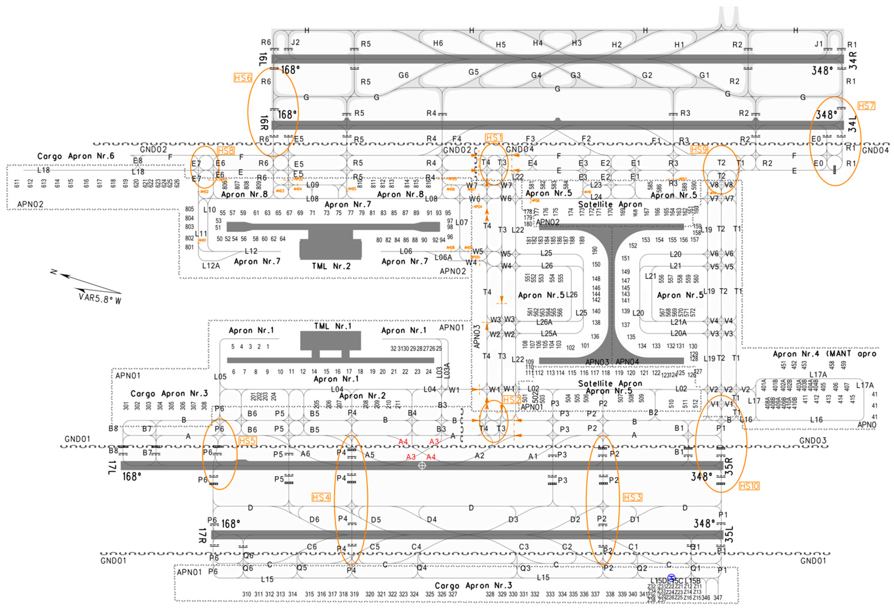
Airport surface operation features include the runway, taxiing distance, number of hotspots (HSs), and runway crossings. The surface layout of PVG is depicted in Figure 2. PVG has four runways: 16L/34R and 17R/35L are primarily used for landings, while 16R/34L and 17L/35R are mainly for takeoffs. The runway feature indicates the specific runway used by the flight for landing, with possible values of 16L, 34R, 17R, or 35L.

The taxiing distance represents the total distance from the landing runway to the assigned stand. The ICAO defines a hotspot as a location on an aerodrome movement area with a history or potential risk of collision or runway incursion, and where heightened attention by pilots/drivers is necessary [23]. PVG’s Aeronautical Information Publication (AIP) defines 10 HSs (see Figure 2), which are high-traffic taxiway intersections or taxiways used for runway crossings. Aircraft may need to slow down or wait at HSs to allow other aircraft to pass before continuing their taxi. By analyzing the taxi path of each flight, we can calculate the number of HSs encountered during taxiing.

Additionally, the number of runway crossings is determined for each flight and included as a feature.

Among these features, only the runway feature is applied in the modeling of both stage 1 and stage 2. This is because the landing runway may influence the aircraft’s entry point into the TMA and its approach flight time, which can vary depending on the runway. In contrast, the remaining three features—taxiing distance, number of HSs, and runway crossings—primarily impact surface operations and do not theoretically affect TMA operations. Therefore, these three features are used only as explanatory variables in stage 2.

3.3. Airport TMA Operation Features

Airport TMA operation features primarily include the height, speed, angle, and flying distance. These features correspond to the altitude of the aircraft upon entering PVG’s TMA, its flight speed, its angle, and the distance between its coordinates (longitude and latitude) and the runway landing point’s coordinates. It is important to note that the construction of airport TMA operation features in this paper did not take into account aircraft holding conditions or missed approaches.

The distance is calculated using the Haversine formula, as shown below:

$$d={\mathrm{s}\mathrm{i}\mathrm{n}}^2\left({\displaystyle \frac{{LAT}_j-{LAT}_i}{2}}\right)+\cos ({LON}_i)\cos ({LON}_j){\mathrm{s}\mathrm{i}\mathrm{n}}^2({\displaystyle \frac{{LON}_j-{LON}_i}{2}})$$

(1)

where d is the distance between two points, and ${LON}_i$, ${LAT}_i$, ${LON}_j$, and ${LAT}_j$ represent the longitude and latitude of point i and point j, respectively.

The ADS-B and A-CDM data from PVG used in this study do not provide the exact time when flights enter the TMA. To determine this, the PNPoly algorithm is employed. This algorithm identifies whether a flight’s trajectory point lies within the TMA. Specifically, each trajectory point is checked sequentially. If trajectory point n is inside the TMA while the preceding point n − 1 is outside, then point n is considered the entry point into the TMA. At this point, the aircraft’s altitude, speed, angle, and flying distance to the runway are recorded as the TMA operational features.

For instance, a portion of the trajectory data for flight MU2536 on 12 October 2022 are shown in

Table 2. Partial trajectory data of flight MU2536.

No.	UTC TIME	Height	Speed	Angle	Location Status
229	2022/10/12 12:27:37	6461.76	779.692	90	0
230	2022/10/12 12:27:52	6362.7	781.544	93	0
231	2022/10/12 12:28:07	6263.64	774.136	99	1
232	2022/10/12 12:28:22	6164.58	768.58	105	1
233	2022/10/12 12:28:37	6065.52	766.728	108	1

. The “Location Status” column indicates whether a trajectory point is inside (1) or outside (0) the TMA. The trajectory of MU2536 is illustrated in Figure 3. The blue line represents the TMA boundary, with the region to the left being outside the TMA and the region to the right inside. The red line shows the flight’s trajectory.

In this example, trajectory point No. 231 is inside the TMA, while the preceding point No. 230 is outside. Hence, point No. 231 is identified as the entry point of MU2536 into the TMA. At this point, the altitude, speed, and angle of the flight are 6263.64 m, 774.136 km/h, and 99°, respectively.

All four airport TMA operation features are exclusively used in the modeling of stage 1.

3.4. Arrival/Departure Flow Features

Arrival and departure flow features encompass the surface arrival traffic flow, surface departure traffic flow, TMA arrival traffic flow, and TMA departure traffic flow. Each of these categories consists of four sub-features, resulting in a total of 4 × 4 = 16 features.

The defined features are as follows:

(1)

Surface arrival traffic flow: A1, A2, A3, and A4

(2)

Surface departure traffic flow: D1, D2, D3, and D4

(3)

TMA arrival traffic flow: AA1, AA2, AA3, and AA4

(4)

TMA departure traffic flow: AD1, AD2, AD3, and AD4

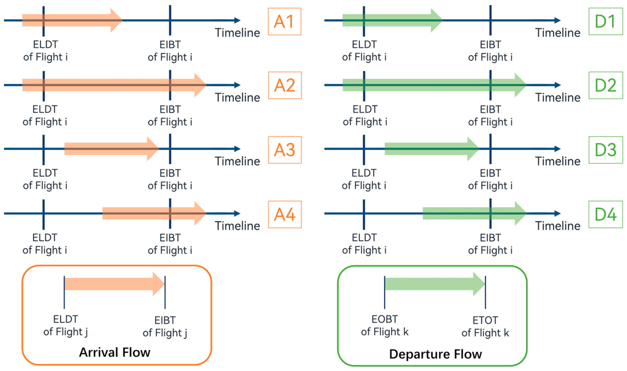
3.4.1. Surface Traffic Flow

Drawing inspiration from the queuing model, surface traffic flow features are introduced into taxi time prediction for the first time [11]. Studies have demonstrated their significant impact on enhancing prediction efficiency across various airports, including PEK [2], MAN and HKG [9], and ARN and ZRH [11]. These features have proven to be effective for improving taxi time prediction models.

Figure 4 clearly portrays the eight defined surface traffic flow features, where the i-th arrival aircraft’s taxiing time is $t_{ELDT}(i),t_{EIBT}(i)$, the j-th arrival aircraft’s taxiing time is $t_{ELDT}(j),t_{EIBT}(j)$, and the k-th departure aircraft’s taxiing time is $t_{EOBT}(k),t_{ETOT}(k)$, where $t_{EOBT}(k)$ is the estimated off-block time and $t_{ETOT}(k)$ is the estimated take-off time. As an example, A1 is defined as the number of all flights j that land before flight i’s ELDT and in-block after flight i’s ELDT but before its EIBT. Similarly, A1–A4 and D1–D4 represent the number of flights j and k operating on PVG’s surface that satisfy the corresponding conditions.

Notably, Idris [24] proposed a method for calculating the number of flights on an airport surface. However, this method relies on determining a flight’s EIBT after it occurs, which is impractical for operational purposes. In real-world scenarios, using actual times for prediction requires waiting until a flight completes taxiing, rendering it ineffective for forward-looking predictions.

In this study, we replace actual times with estimated times for prediction purposes. Since an aircraft’s AIBT is only known post-taxiing, predictions based on actual times would involve a delay until after in-block completion, defeating the purpose of proactive planning.

Moreover, during periods of high surface activity, the number of waiting aircraft on the surface may influence aircraft landing within the TMA. Consequently, surface traffic flow can also impact the approach flight time in stage 1. Hence, all eight surface traffic flow features are incorporated as explanatory variables in both stage 1 and stage 2 models.

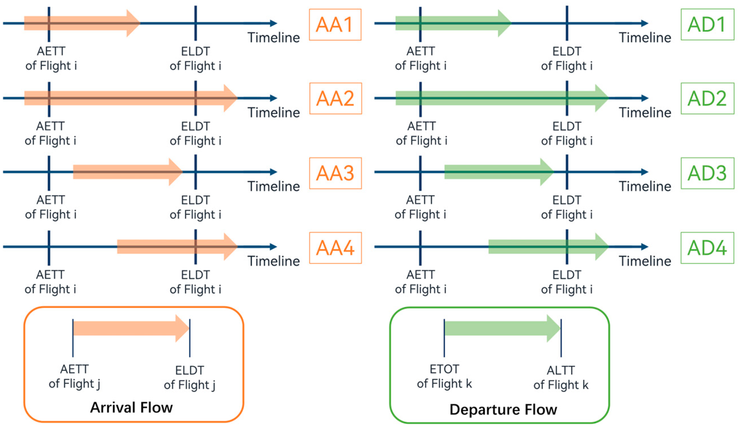
3.4.2. TMA Traffic Flow

Building on the concept of surface traffic flow, we propose eight airspace traffic flow features: four airspace arrival flow features (AA1–AA4) and four airspace departure flow features (AD1–AD4). As illustrated in Figure 5, we define the i-th arriving aircraft’s approach flight time as $t_{AETT}(i),t_{ELDT}(i)$, the j-th arriving aircraft’s approach flight time as $t_{AETT}(j),t_{ELDT}(j)$, and the k-th departing aircraft’s approach flight time is $t_{ETOT}(k),t_{ALTT}(k)$, where $t_{AETT}$ is the actual time when the aircraft enters the TMA and $t_{ALTT}$ is the actual time when the aircraft leaves the TMA. For instance, AD1 is defined as the number of all flights k that take off before the actual enter the TMA time (AETT) of flight i, and leave the TMA after flight i’s AETT and before its ELDT. Similarly, the values of AA1–AA4 and AD1–AD4 represent the number of flights j and k operating in the TMA of PVG that meet the specified conditions.

Unlike surface traffic flow, the calculation of TMA traffic flow relies on two actual times, the AETT and actual leave the TMA time (ALTT), as the ADS-B data provide only these actual timestamps for aircraft entering and leaving the TMA. Estimated times for these events are not available in the dataset.

Additionally, a high TMA traffic density often corresponds to a greater number of arriving and departing aircraft. This congestion may lead to conflicts with arriving flights on the surface, thereby impacting their taxiing time. Consequently, all eight TMA traffic flow features are included as explanatory variables in both stage 1 and stage 2 models.

3.5. Weather Features

Weather plays a significant role in TMA operations as it can influence an aircraft’s performance, trajectory, and sequencing intervals, thereby indirectly affecting approach flight times [7]. For surface operations, most existing studies have not identified a strong correlation between weather conditions and taxi times [25,26,27]. However, due to variations in airport size and configuration, this study includes weather features to examine their potential impact on surface taxiing times.

A binary weather feature is defined to indicate the presence of severe weather, such as thunderstorms or rainfall, on the day of aircraft operations. A value of 1 represents the presence of severe weather, while 0 denotes its absence.

Given the potential impact of weather on both airspace and surface operations, this feature is included as an explanatory variable in both stage 1 and stage 2 models.

4. Methodology

This section introduces the concept of copula entropy for feature selection based on dependency measures. Additionally, the LightGBM model is employed to predict the approach flight time, taxi-in time, and taxi-out time. The model’s performance is evaluated and compared using five key metrics.

4.1. Copula Entropy

Copula entropy is a multivariate statistical independence measure proposed by Ma [19]. Similar to the Pearson correlation coefficient, copula entropy is also used to measure the dependence between variables. However, copula entropy has no requirement for the distribution of data. Therefore, copula entropy can be better applied in more fields than the Pearson correlation coefficient.

Based on Sklar’s theorem, copula entropy can be represented as a product of its marginals and the copula density function. The copula density represents the dependence structure between variables. Copula entropy is defined as follows:

$$H_c(\mathit{X})=-{\int }_{u}c\left(\mathit{u}\right)\ln c\left(\mathit{u}\right)d\mathit{u}$$

(2)

where X is the random variable and u and c(u) are the marginal distributions and copula density of the random variable X, respectively.

The copula entropy-based variable selection method has been shown to optimize the prediction results of machine learning models, and it has also been verified to outperform traditional variable selection methods such as Lasso and stepwise regression in terms of variable selection [28]. In this paper, we will measure the copula entropy of each feature in the two-stage model and use copula entropy as a criterion for variable selection in order to obtain a prediction model with better performance while giving some accuracy to our prediction model. In this paper, we will use the “copent” package of the R language to calculate the copula entropy of the features.

4.2. LightGBM

LightGBM is a gradient-boosting framework that uses tree-based learning algorithms. It is designed to be efficient and can handle large-scale data. Unlike other boosting methods, LightGBM uses a leaf-wise tree growth algorithm, which can reduce the number of splits and improve the overall computational efficiency. At each iteration of the training process, LightGBM selects the most significant feature to split on and grows the tree in a bottom-up manner until reaching the maximum leaf nodes or reaching the minimum loss reduction threshold. Additionally, LightGBM supports histogram-based algorithms for faster computation and provides user-defined loss functions for flexible optimization.

Both GBRT and XGBoost algorithms, similar to LightGBM, have been widely used in the fields of approach flight time prediction [10] and surface taxi time prediction [9,29]. In this paper, we use the “lightgbm” library in Python 3.12 to build a LightGBM model to predict the approach flight time, taxi-in time, and integrated arrival time of an aircraft. As a decision tree regression model, LightGBM does not require the feature dimensions, so the data used in this paper do not require one-hot-encoding and normalization; therefore, some information on the classification features can be retained to the maximum extent.

4.3. Performance Metrics

The performance metrics chosen in this paper include $R^2$, $RMSE$, and prediction accuracy.

4.3.1. $R^2$

$R^2$ is the coefficient of determination, which indicates the degree to which the explanatory variables explain the response variables. The value of $R^2$ is between [0,1], and the closer it is to 1, the better the model fits. The definition of $R^2$ is as follows:

$$R^2=1-{\displaystyle \frac{{\sum }_i{({\widehat{y}}_i-y_i)}^2}{{\sum }_i{(y_i-\overline{y})}^2}}$$

(3)

where $y_i$ is the actual value of the response variable, ${\widehat{y}}_i$ is the predicted value, and $\overline{y}$ is the mean value of the response variable.

4.3.2. $RMSE$

$RMSE$ is an important metric for assessing the performance of a model. It amplifies the difference between larger errors. The smaller the value of $RMSE$, the better the performance of the model. The $RMSE$ is defined as follows:

$$RMSE=\sqrt{{\displaystyle \frac{1}{m}}\sum _{i=1}^m{({\widehat{y}}_i-y_i)}^2}$$

(4)

4.3.3. Prediction Accuracy

In the actual prediction of approach flight times, airports are more interested in the error between the predicted values and actual values. We introduce a prediction accuracy metric, whose value is the ratio of the number of differences between the model output and the actual approach flight time within a set range to the total number of predicted samples. Here, we set the prediction accuracy in the range of 1, 3, 5, and 10 min, respectively.

5. Results

In this section, we begin by performing variable selection using copula entropy as the criterion. Next, LightGBM models are developed for prediction, and their performances are compared across different models. Finally, we attempt to interpret the results of the models.

5.1. Variable Selection Based on Copula Entropy

To facilitate comparison, the data were divided into three groups: stage 1, which includes features related to the approach flight stage, with the response variable being the approach flight time; stage 2, which focuses on the taxi-in stage, with the response variable being the taxi-in time; and the overall group, which combines all features, with the response variable being the integrated arrival time.

Figure 6 illustrates the feature selection process for each group, where the copula entropy values of “Weather”, “Time period”, and “AA1” serve as thresholds for the stage 1, stage 2, and overall groups, respectively. These thresholds, marked as red lines in the figure, determine the inclusion of variables in the model based on whether their copula entropy values exceed the threshold. We used the $RMSE$ of the model results as the optimization objective and determined the optimal threshold through cross-validation [30,31]. The selected features for each group are summarized in

Table 3. Selected features by Copula Entropy.

Stage	Selected Variables
Stage 1	Time period, Runway, Height, Speed, Angle, Flying distance, A1, A3, A4, AA1, AA2, AA3, AA4, AD4, Weather
Stage 2	Base airlines, Aircraft types, Time period, Runway, Distance, Number of HS, A1, A2, A3, A4, AA1, AA2, AA3, AA4
Overall	Aircraft types, Time period, Runway, Distance, Number of HS, Height, Speed, Angle, Flying distance, A1, A2, A3, A4, AA3, AA4

.

The results indicate that flight distance and taxiing distance are the most important features for the first and second stages, respectively, as longer distances naturally require more time. In the first stage, features such as altitude, speed, and angle are particularly relevant, suggesting that the speed and altitude of the aircraft when entering the TMA are the primary factors influencing the model’s prediction accuracy. In practical operations, a higher flight altitude or slower speed at the approach flight point implies that the aircraft’s approach process will require more time, i.e., a longer approach flight time. In the second stage, the number of hotspots is a critical feature, as a higher number of hotspots increases the likelihood of conflicts during taxiing. This finding aligns with observations by Zhao [29] and Kim [27]. Additionally, among categorical features, runway and aircraft type have relatively high importance. Regarding runways, there are significant differences in the approach flight times of aircraft landing on different runways at PVG. As for aircraft types, different models exhibit notable variations in speed during the entire approach process, thereby significantly impacting the approach flight time.

However, the departure flow characteristics were largely excluded from the model, which may be attributed to the operational features of PVG. The commissioning of the fourth runway in 2015 [32] led to a clear separation between arrival and departure operations. Arrival flights predominantly utilize runways 16L/34R and 17R/35L, whereas departure flights primarily rely on runways 16R/34L and 17L/35R. This separation effectively minimizes conflicts between arriving and departing flights on the surface and within the TMA.

The results also reveal that weather features were selected for the first stage of the model but excluded from the second stage. This suggests that adverse weather conditions, such as rainfall and haze, reduce visibility and slow aircraft speeds, thereby significantly impacting the approach flight time.

5.2. Results of the LightGBM Model

To evaluate the performance of the LightGBM model, we trained it using 80% of the data and reserved the remaining 20% for testing. Model training involved 10-fold cross-validation to identify optimal parameters, ensuring fairness by using consistent random seeds across all models for data splitting and parameter initialization. This standardization allows for a robust comparison of results between different models.

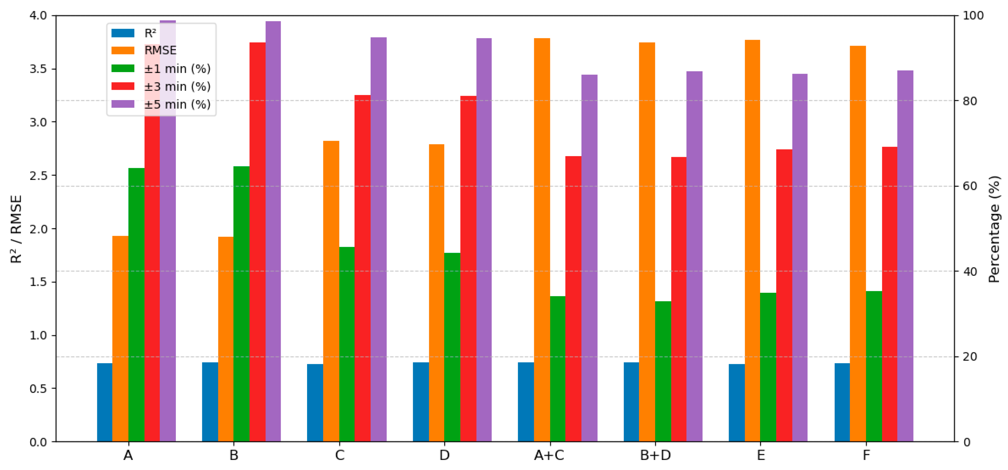
To assess the impact of copula entropy-based feature selection on model optimization, six groups of models were constructed using the three datasets described in

Table 4. Description of each group of models.

Group	Response Variable	Explanatory Variables
A	Approach flight times	All features
B	Approach flight times	Features in stage 1 of Table 3
C	Taxi-in times	All features
D	Taxi-in times	Features in stage 2 of Table 3
E	Integrated arrival times	All features
F	Integrated arrival times	Features in overall of Table 3

. The performance of each model is summarized in

Table 5. Prediction results of the LightGBM model.

Metrics	A	B	C	D	A + C	B + D	E	F
$R^2$	0.737	0.740	0.727	0.740	0.741	0.745	0.730	0.733
$RMSE$	1.93	1.92	2.82	2.79	3.78	3.74	3.77	3.71
±1 min (%)	64.17	64.61	45.60	44.29	34.03	32.99	34.79	35.34
±3 min (%)	93.23	93.68	81.21	81.03	66.85	66.68	68.60	69.09
±5 min (%)	98.74	98.58	94.81	94.65	86.02	86.73	86.29	87.11

and Figure 7. Groups A and B are compared to evaluate the effect of feature selection on predicting approach flight times, while groups C and D are compared for taxi-in times. Groups E, F, A + C, and B + D are analyzed to assess the overall model performance. Notably, A + C and B + D represent the combined predictions of groups A and C and groups B and D, respectively. For clarity, the best performance in each comparison is highlighted in bold.

A comparison of groups A and B reveals that the copula entropy-based feature selection (group B) improves prediction accuracy. Conversely, for groups C and D, the model with all features (group C) slightly outperforms the feature-selected model (group D). Despite this, copula entropy demonstrates its strength in improving model interpretability and optimizing stage 1 predictions. However, in stage 2, the focus on $R^2$ as a training metric may have led to a diminished emphasis on prediction accuracy.

In the comparison of groups A + C, B + D, E, and F, feature selection using copula entropy proves advantageous, with group F achieving the best performance in both prediction accuracy and $RMSE$. Interestingly, group B + D, representing split-stage prediction, achieves the highest $R^2$. This outcome can be attributed to the treatment of the two stages as independent components; when combined, their variances add up, resulting in a recalibrated distribution that enhances $R^2$. This finding suggests that for machine learning models prioritizing predictive accuracy over interpretability, treating the two stages as an integrated system can yield better results.

Despite these insights, the maximum prediction accuracy of the two-stage model reaches only 87.11%. Several factors may contribute to this gap. First, the unique operational configuration of PVG—with its four runways segregating arrival and departure flights—reduces surface traffic conflicts, limiting the relevance of certain features. Second, PVG’s high traffic volume and complex surface and TMA dynamics may challenge model precision. Finally, the shared TMA between PVG and Shanghai Hongqiao International Airport (SHA) introduces uncertainties regarding the influence of SHA’s flights on the predictions.

6. Conclusions

The two-stage integrated prediction of aircraft arrival time is crucial for improving airport management efficiency. This study combines the prediction of approach flight time and taxi-in time, proposing a method that clearly defines the criteria for dividing the two stages. By designing features based on the TMA and ground operations tailored to the configuration characteristics of PVG and integrating the copula entropy-based variable selection method with the LightGBM model, we analyze influencing factors and predict the integrated arrival time, thereby validating the applicability of this method.

A key focus of this study is the construction of a two-stage LightGBM prediction model. The results show that the accuracy of stage-specific predictions is lower than that of two-stage integrated prediction. Notably, the two-stage LightGBM model achieves a prediction accuracy of nearly 70% within a ±3 min range and close to 90% within a ±5 min range. In actual airport operations, the appropriate prediction model can be flexibly selected based on specific needs. For example, when the requirement for early predictions of arrival time is not high (e.g., after flight landing), a standalone approach flight time prediction model or taxi-in time prediction model can be chosen to meet basic needs. If higher requirements for prediction timing and in-depth analyses of influencing factors are needed, the two-stage prediction model can be prioritized. In cases where overall model prediction performance is more critical, integrated arrival time can be selected as the prediction target to achieve better results.

Another focus of this study is the use of copula entropy to compare feature importance. The results reveal that, due to the unique configuration of PVG, departure traffic flow has a minimal impact on approach flight time and taxi-in time. This highlights the importance of identifying airport-specific features when selecting features for prediction models. For multi-runway airports such as PVG, where arrival and departure operations are separated, further research into surface traffic flow and TMA flow is essential to improve prediction accuracy. Additionally, copula entropy effectively enhances the accuracy of prediction models, particularly in the feature selection process. Capturing nonlinear correlations and high-dimensional interactions between variables reduces the interference of redundant features, thereby optimizing the model’s generalization capability and predictive performance.

Although this study has achieved certain results in the field of EIBT prediction, there are still areas worthy of further exploration. For example, future research could leverage existing ADS-B data to identify missed approaches and holding patterns [33], further refining the construction of operational features for flights in the terminal area, thereby more comprehensively reflecting real-world scenarios in complex operational environments. Furthermore, while this study validates the effectiveness of LightGBM and the copula entropy-based variable selection method at PVG, its applicability to other airports requires further investigation. Additionally, future research could incorporate more detailed weather data to better characterize the influence of weather factors, such as pavement conditions (dry/wet/flooded/snow-covered, etc.), seasonal variations, and extreme weather conditions, on taxiing speeds.