Exploring the Design Space of Low-Thrust Transfers with Ballistic Terminal Coast Segments in Cis-Lunar Space

Abstract

Spacecraft catering to the Lunar Gateway or other “permanent” stations in the lunar vicinity would require frequent travel between periodic orbits around the Earth–Moon $L_1$ and $L_2$ Lagrange points. The transition through the Hill sphere is often characterized by close passages of our nearest neighbor—rendering the optimization problem numerically challenging due to the increased local sensitivities. Depending on the mission requirements and resource constraints, transfer architectures must be studied, and trade-offs between flight time and fuel consumption quantified. While direct low-thrust transfers between the circular restricted three-body problem periodic orbit families have been studied, the asymptotic flow in the neighborhood of the periodic orbits could be leveraged for expansion and densification of the solution space. This paper presents an approach to achieve a dense mapping of manifold-assisted, low-thrust transfers based on initial and terminal coast segments. Continuation schemes are utilized to attain the powered intermediate time-optimal segment through a multi-shooting approach. Interesting insights regarding the linear correlation between $\Delta$V and change in reduced two-body osculating elements associated with the initial-terminal conditions are discussed. These insights could inform the subsequent filtering of the osculating selenocentric periapsis map and provide additional interesting and efficient solutions. The described approach is anticipated to be extremely useful for future crewed and robotic cis-lunar operations.

1. Introduction

The 21st-century edition of the so-called “Space Race” is well underway, and establishing sustained human presence in the vicinity of our planet’s only moon is at the forefront of space mission objectives. In addition to learning more about our origins through science experiments, the idea of sustainability is founded on effective in situ resource utilization to avoid expensive round trips back home. Technology demonstrations leading to eventual crewed explorations are underway with NASA’s Artemis missions [1]. The global space community plans to construct a lunar space station, akin to the International Space Station (ISS), with a member of the near-rectilinear halo orbit family around the $L_2$ Lagrange point earmarked for operation [2]. With a further increase in global collaboration in the future, other libration point orbits (LPOs) would inevitably be utilized as destination orbits for similar “stations” or as observation orbits for space domain awareness (SDA) applications. Frequent trips for spacecraft across the Earth–Moon $L_1$ to $L_2$ region would be required to cater to a variety of operational needs, growing with the increasing human presence.

LPOs are periodic constructs around equilibrium points that are admitted by the circular restricted three-body problem (CR3BP) dynamical system. Historically, the existence of periodic orbit families has been a boon for space missions, such as SOHO [3], JWST [4], etc., where the unique orbit properties have been leveraged to design mission architectures capable of satiating ambitious and disruptive science objectives [5]. Although analyzing the three-body problem with the “circular” and “restricted mass” assumptions is necessary for the existence of LPOs and the associated structures, for realism and improved accuracy, other dynamical systems are often studied: elliptical restricted three-body problem (ER3BP) [6,7], bi-circular restricted four-body problem (BCR4BP) [8,9], and higher-fidelity models (HFM) [10,11]. Invariant manifolds in the CR3BP are LPO-associated characteristic structures that capture the local asymptotic flow wound fixed points on the periodic orbit. The boundaries of these stable and unstable manifolds, known as Lagrangian coherent structures (LCS), segregate the local dynamical behavior. Due to their asymptotic nature, the inherent stability of the LPO massively affects the manifold dynamics. In the CR3BP, both the planar and 3-D LCS structures have been analyzed to determine the stability of various orbits in several three-body systems [12,13]. Novel methods for computing these trajectories have been studied along with parallelization schemes [14,15,16,17]. Additionally, the secular evolution of these structures could be leveraged to assist in both insertion and departure transfers between LPOs. For such scenarios, the spacecraft coasts along the unstable manifold to facilitate a “natural” departure from the initial LPO, which is either followed by a powered phase or a ballistic connection with the stable manifold of the destination LPO (heteroclinic connections) [18,19,20,21].

When allowed to continue indefinitely, the manifolds from one periodic orbit may intersect either with themselves or with those of another orbit. These position junctions have become known as homo-clinic and hetero-clinic connections, respectively. These connections are extremely rare due to the chaotic nature of the manifolds but are also extremely useful for mission design. The corresponding trajectories have been previously leveraged to transfer between various periodic orbits. By using Poincaré maps and analyzing stability connections, successful transfers between orbits have been made in the CR3BP. Such transfers have been discovered and leveraged within the Sun–Jupiter system, particularly for planar Lyapunov orbits [20]. Intersection between the stable and unstable manifolds of the orbits create such connections, which allow for relatively cost-effective maneuvering.

If a hetero-clinic connection is present, then the spacecraft can essentially “drift” from one orbit to the next. However, as mentioned, these connections are exceedingly rare; instead, finding a manifold’s near misses and using a small amount of $\Delta v$ to adjust is much more feasible. In any case, the potential for using manifolds as a means to transfer between orbits has been studied substantially [8,17,18,19,22,23,24,25]. Both impulsive and low-thrust schemes in the CR3BP were analyzed in these instances, with each having their own benefits and drawbacks; some of these have been previously used in the context of interplanetary transfers [26]. Comparisons between the CR3BP and BCR4BP have been performed to quantify the influence of the Sun on the manifold structures of the Earth–Moon system [27]. Some analyses have proposed transfers of low-thrust spacecraft to halo orbit invariant manifolds within the CR3BP and BCR4BP [8,23,28]. The low-thrust trajectories developed in the CR3BP have also been used as a warm start to assist numerical convergence in an HFM for specific cases and orbits [24,29].

Trajectory optimization for a spacecraft equipped with a low-thrust engine has also been well studied using direct and indirect approaches [30,31,32,33,34]. The ensuing two-point boundary value problem (TPBVP) can be numerically solved using the shooting method. Typically, multi-rev solutions that are characteristic of spacecraft starting deep in the central body gravity well require additional numerical techniques to rigorously achieve convergence [35]. In the context of the CR3BP, challenges with numerical convergence are expected near to either the primary or the secondary. The TPBVP can be made more amenable to numerical treatment by using a multiple-shooting approach. Time-optimal solutions are typically continuous thrust and minimize the time of flight while solving for an optimal thrusting direction. Low-thrust spacecraft have been simulated in the CR3BP to transfer from various locations to periodic orbits [22,23,36]. Fuel costs were quantified for these low-thrust transfers between the five liberation points capturing the overall trends as the Jacobi constant values are altered [23]. While manifold-driven low-thrust transfers have been explored in the context of the Earth–Moon CR3BP in general, most studies have been either concerned with finding hetero-clinical connections and approximating the fuel cost by simulating an impulsive maneuver to bridge the velocity mismatch or been limited to particular solutions using specific manifold trajectories associated with selected LPOs for low-thrust transfer. The transition through the Hill sphere in the Earth-Moon system poses significant numerical challenges. This has only led to a sparse mapping of the solution space, painting an incomplete picture of the underlying trade-offs and the interplay between time of flight and fuel consumption.

In this paper, we aim to bridge the identified gaps and present a methodology that provides interesting insights into manifold-driven transfers from ${\mathrm{EML}}_1$ to ${\mathrm{EML}}_2$ periodic orbits. In particular, our aims are as follows:

1.

Demonstrate an approach to map the dense solution space over the entire manifold bundle for a “COAST-THRUST-COAST” transfer, with the COAST segments indicating travel along the manifolds for non-planar periodic orbits.

2.

Quantify a geometrically coherent domain corresponding to fuel savings for the chosen transfer type.

3.

Estimate the linear correlation between fuel consumption and time of flight for osculating conditions using a restricted two-body model.

4.

Gain insights to select the targeting states from a library of osculating conditions to maximize fuel efficiency.

It is shown that a combination of multiple-shooting, parameter continuation, judicious choice of the coordinate system, and efficient boundary condition filtering can mitigate most convergence challenges. The rest of the paper is organized as follows: Section 1 and Section 2 discuss the theory and preliminaries. Section 3 describes the architecture for designing time-optimal powered segments that leverage the asymptotic behavior of invariant manifolds for more fuel-efficient transfers. Section 4 presents the results pertaining to filtered manifold boundary conditions, direct transfers, and transfers that leverage the filtered condition. Section 5 concludes the paper by elucidating key results and discussing avenues for future work.

2. Preliminaries

2.1. Circular Restricted Three Body Problem

The circular restricted three-body problem (CR3BP) is an astrodynamical system where the motion of a restricted third body, $m_3$, is affected gravitationally by a primary–secondary pair, $m_1$ and $m_2$, respectively. The two larger bodies exhibit circular Keplerian motion about their barycenter. Thus, their distances with the barycenter, $d_1$ and $d_2$, remain unchanged. As such, the system is autonomous when the dynamics are analyzed in a synodic rotating frame. The Hamiltonian nature allows for time-invariant analyses of regions near the Lagrange points and associated periodic orbit families.

The barycentric rotating frame and its basis vectors -$\{x,y,z\}$ are more appropriate for modeling the dynamics as seen in Figure 1. For computational efficiency, the three-body system is normalized to have a mass ratio, $\mu$, that defines the secondary mass contribution with the total system mass set as 1 (i.e., $1-\mu$ is the primary mass contribution). Furthermore, the radius defines the length unit $\left(LU\right)$ and period is normalized by $2\pi$ to define the time unit $\left(TU\right)$. As such, the rotation rate is constant and set to 1 with Szebehely’s equations, as presented in [37]:

$$\begin{array}{cc}\hfill \ddot{x}& =x+2\dot{y}-{\displaystyle \frac{(1-\mu )(x+\mu )}{r_1^3}}-{\displaystyle \frac{\mu (x-1+\mu )}{r_2^3}},\hfill \end{array}$$

(1a)

$$\begin{array}{cc}\hfill \ddot{y}& =y-2\dot{x}-\left({\displaystyle \frac{1-\mu }{r_1^3}}+{\displaystyle \frac{\mu }{r_2^3}}\right)y,\hfill \end{array}$$

(1b)

$$\begin{array}{cc}\hfill \ddot{z}& =-\left({\displaystyle \frac{1-\mu }{r_1^3}}+{\displaystyle \frac{\mu }{r_2^3}}\right)z,\hfill \end{array}$$

(1c)

where the dot (˙) indicates time derivatives with the following distance definitions for the third body:

$$\begin{array}{cc}\hfill r_1& =\sqrt{{(x+\mu )}^2+y^2+z^2},\hfill \end{array}$$

(2a)

$$\begin{array}{cc}\hfill r_2& =\sqrt{{(x-1+\mu )}^2+y^2+z^2}.\hfill \end{array}$$

(2b)

The CR3BP admits five equilibrium points (Lagrange points), and the existence of periodic orbits is well established. Additionally, the Jacobi integral (C) is a constant of motion that defines iso-energy contours. C in conjunction with the state transition matrix (STM) can be analyzed to derive stability metrics for the orbits. In the context of the Earth–Moon system, $\mu =1.215058560962404\times {10}^{-2}$, 1 $LU$ = 389,703 km, and 1 $TU$ = 382,981 is consistent with the Three-Body Periodic Orbit Database [38]. The initial conditions for periodic orbit families used in this paper were obtained from this database. Typically, these orbits are unstable, and the CR3BP dynamical system is chaotic. Therefore, any initial deviation (forced or unforced) will cause a departure from nominal behavior.

It is hereby noted that assuming coincident inertial and rotating frames at the start of propagation simplifies any subsequent state transformations. This is easily captured through a rotation about the z-axis following a translation to the chosen ‘new’ origin along the x-axis. Further determination of the osculating classical orbital elements in a restricted two-body Moon–spacecraft system is straightforward through careful conversion from canonical to real units.

2.2. Invariant Manifolds

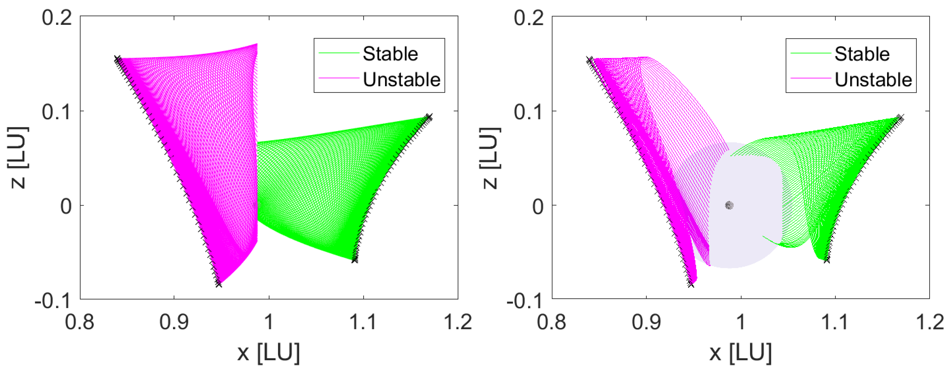
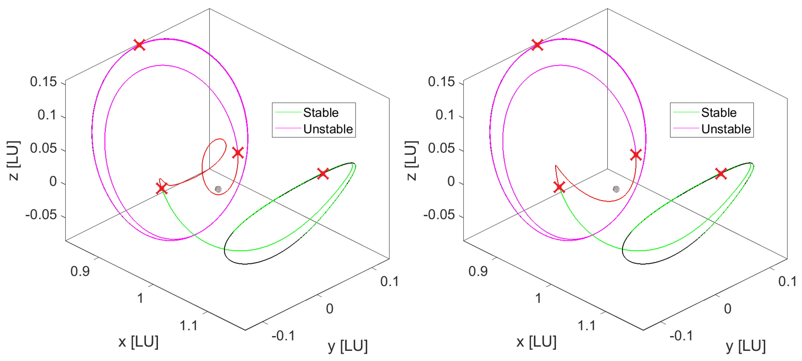
Invariant manifolds are dynamical system constructs that characterize the asymptotic flow in the neighborhood of a hyperbolic fixed point on a periodic orbit. Analyzing them is pertinent to characterizing local behaviors that occur naturally. Performing an eigenanalysis on the monodromy matrix, i.e., the linearized STM after one period, of the selected periodic orbit reveals the local eigenvalues and the corresponding eigenvectors in pairs. The eigenvectors associated with the largest and smallest real eigenvalues (reciprocals in the CR3BP) represent the respective directions for the unstable and stable manifolds (see Figure 2).

Embedded in traditional dynamical system analysis is the concept of hetero-clinical connections, which have been extensively analyzed [20]. These connections unearth natural pathways in space that can be leveraged to design low-energy transfers across LPOs. After the spacecraft departs the original periodic orbit and traverses on the unstable manifold, only a single impulse is necessary at the position intersection point to alter the direction and rendezvous with the stable manifold. An instantaneous correction via impulsive maneuver is generally inefficient. Nevertheless, such a thrusting profile can easily be generated as a “control group” when comparing alternatives. As previously mentioned, multiple studies have combined and compared transfers between various orbits in the CR3BP using these techniques. The overall transfer cost can be further reduced due to the judicious leverage of the gravitational field and naturally occurring dynamics, as well as by using more efficient propulsion systems.

2.3. Indirect Approach to Optimal Control of Continuous Systems

Analysis of continuous systems in the context of finding a stationary condition for a predefined cost function requires calculus of variations [39]. Considering a system described by a set of nonlinear ordinary differential equations ($\mathbf{X}\in {\mathbb{R}}^n$ and $\mathbf{u}\in {\mathbb{R}}^m$):

$$\dot{\mathbf{X}}=\mathit{f}(\mathbf{X},\mathbf{u},t),\forall t\in [t_0,t_f],$$

(3)

where $\mathbf{X}$ defines the state-space of the dynamical system and $\mathbf{u}$ denotes the control inputs. The initial value problem is well defined, i.e., $\mathbf{X}\left(t_0\right)={\mathbf{X}}_{\mathbf{0}}$ is given/known. Let the cost function or performance index be defined as

$$J=\varphi (\mathbf{X}\left(t_f\right),t_f)+{\int }_{t_0}^{t_f}L(\mathbf{X}\left(t\right),\mathbf{u}\left(t\right),t)dt.$$

(4)

Note that $\varphi$ denotes the “terminal cost”, while the integral term denotes the “running cost” using the Lagrangian L. The Lagrange multiplier ($\Lambda \in {\mathbb{R}}^n$) approach is used to define an updated performance index ($\overline{J}$), which levies a running cost as the system departs from the underlying physics under the action of any non-stationary control function $\mathbf{u}\left(t\right)$. $\overline{J}$ is defined as

$$\overline{J}=\varphi (\mathbf{X}\left(t_f\right),t_f)+{\int }_{t_0}^{t_f}[L(\mathbf{X}\left(t\right),\mathbf{u}\left(t\right),t)+{\Lambda }^T\{\mathit{f}-\dot{\mathbf{X}}\}]dt.$$

(5)

Generally, the Hamiltonian function is defined as $\mathrm{H}(\mathbf{X},\mathbf{u},\Lambda ,t)=L+{\Lambda }^T\mathit{f}$. Substituting H in Equation (3) and finding the first variation of the updated cost function -$\delta \overline{J}$ provides the analytical first-order optimality (stationarity) conditions, known as the Euler–Lagrange equations and mathematically represented as

$$\begin{array}{c}{\dot{\Lambda }}^T=-{\displaystyle \frac{\partial \mathrm{H}}{\partial \mathbf{X}}}=-{\displaystyle \frac{\partial L}{\partial \mathbf{X}}}-{\Lambda }^T{\displaystyle \frac{\partial \mathit{f}}{\partial \mathbf{X}}};\mathrm{such}\mathrm{that},{\Lambda }^T\left(t_f\right)={\displaystyle \frac{\partial \varphi }{\partial \mathbf{X}\left(t_f\right)}}\end{array}$$

(6)

$$\begin{array}{c}{\displaystyle \frac{\partial \mathrm{H}}{\partial \mathbf{u}}}=\mathbf{0}.\end{array}$$

(7)

Equations (3) and (6) give the so-called state-adjoint system of differential equations, which must be solved by determining the optimal control using Equation (7). Note that the conditions for this problem as posed are only partially defined at either boundary ($t_0$ OR $t_f$). The known boundary conditions for the described TPBVP, as stated, are as follows: at $t_0$, $\mathbf{X}\left(t_0\right)$ is known, and at $t_f$, ${\Lambda }^T\left(t_f\right)$ is known (Equation (6)).

The formulation described above is generic, but it must be noted that the dynamical system’s state-space description, the governing physics, and the choice of performance criteria may lead to several sub-classes of the general optimal control problem. For instance, consider a continuous system where some state variables are specified at the final time, $t_f$. Circling back, the first variation of $\overline{J}$ can be mathematically described as

$$\delta \overline{J}={\left[\left({\displaystyle \frac{\partial \varphi }{\partial \mathbf{X}}}-{\Lambda }^T\right)\delta \mathbf{X}\right]}_{t=t_f}+{\left[{\Lambda }^T\delta \mathbf{X}\right]}_{t=t_0}+{\int }_{t_0}^{t_f}\left[\left({\displaystyle \frac{\partial \mathrm{H}}{\partial \mathbf{X}}}+{\dot{\Lambda }}^T\right)\delta \mathbf{X}+{\displaystyle \frac{\partial \mathrm{H}}{\partial \mathbf{u}}}\delta \mathbf{u}\right]dt.$$

(8)

Now, given that some subset of the system states are prescribed at $t_f$, the variation of this subset at the final time must be 0. Therefore, the boundary conditions on $\Lambda$ from Equation (6) are only partially defined in this case. This leads to a trade-off between the co-state boundary and state boundary conditions when the generic problem is morphed into the more specific problem described above. More generally, the problem might require constraining a function of the terminal states, rather than the terminal states themselves. Let $\psi (\mathbf{X}\left(t_f\right),t_f)$ denote the set of such constraint functions such that $\psi$ is a q-vector. For such problems, the updated performance index will typically require two sets of Lagrange multipliers, ${\nu }^T\in {\mathbb{R}}^q$ and ${\Lambda }^T\in {\mathbb{R}}^n$, and can be written as

$$\overline{J}=\Phi (\mathbf{X}\left(t_f\right),\nu ,t_f)+{\int }_{t_0}^{t_f}[L(\mathbf{X}\left(t\right),\mathbf{u}\left(t\right),t)+{\Lambda }^T\{\mathit{f}-\dot{\mathbf{X}}\}]dt,$$

(9)

where the function $\Phi$ is given by

$$\Phi =\varphi +{\nu }^T\psi .$$

(10)

The first-order necessary conditions for $\overline{J}$ to have a stationary value can be summarized as

$$\left\{\begin{array}{cc}\hfill \dot{\mathbf{X}}& =\mathit{f}(\mathbf{X},\mathbf{u},t)\left(n\mathrm{diff}.\mathrm{eq}.\right)\hfill \\ \hfill {\dot{\Lambda }}^T& =-{\displaystyle \frac{\partial \mathrm{H}}{\partial \mathbf{X}}}\left(n\mathrm{diff}.\mathrm{eq}.\right)\hfill \\ \hfill {\displaystyle \frac{\partial \mathrm{H}}{\partial \mathbf{u}}}& =\mathbf{0}\left(m\mathrm{algebraic}\mathrm{eq}.\right)\hfill \\ \hfill X_k\left(t_0\right)& \mathrm{given}\mathrm{or}{\lambda }_k\left(t_0\right)=0\forall k=1\cdots n\hfill \\ & \left(n\mathrm{boundary}\mathrm{conditions}\right)\hfill \\ \hfill {\Lambda }^T\left(t_f\right)& ={\left({\displaystyle \frac{\partial \varphi }{\partial \mathbf{X}}}+{\nu }^T{\displaystyle \frac{\partial \psi }{\partial \mathbf{X}}}\right)}_{t=t_f}\hfill \\ & \left(n\mathrm{boundary}\mathrm{conditions}\right)\hfill \\ \hfill \psi (\mathbf{X}\left(t_f\right),t_f)& =0\left(q\mathrm{side}\mathrm{conditions}\right)\hfill \end{array}\right.$$

(11)

The m algebraic equations can be solved to find the optimal control, the m-vector $\mathbf{u}\left(t\right)$. The state-adjoint system has $2n$ different equations with $2n$ boundary conditions, as stated above. The new set of unknown Lagrange multipliers ($\nu$) can be found using the terminal boundary conditions such that they satisfy the “side conditions”. The TPBVP as stated is amenable to numerical treatment by using a non-linear system solver that minimizes the residual function (defined using the boundary conditions), while the augmented system is propagated from $t_0$ to $t_f$ using the optimal control function ${\mathbf{u}}^{*}\left(t\right)$.

2.4. Two-Point Boundary Value Problem

Ideally, for the two-point boundary value problem (TPBVP) in the context of spacecraft trajectory design using an indirect approach, the departure and arrival states are well defined. These correspond to the position and velocity of the spacecraft at the boundaries, and as such, any arbitrary path can only be obtained through a control profile. The trajectory satisfying these boundary conditions at both ends while minimizing the cost function follows an optimal control profile. For the simplest solution approach, since the co-states are unknown at $t_0$, they are guessed and iteratively solved numerically. Certain collocation approaches use uniform trigonometrization to solve the TPBVP. In this case, shooting methods are employed as they guarantee optimality and are discussed below.

2.4.1. Single-Shooting

In the CR3BP, due to the time-invariant nature, the system and state representation are autonomous. The simplest method for finding a trajectory that traverses the desired path based on thrust inputs is a single-shooting scheme. Since the initial state is known, a fixed-free condition is utilized whereby only the co-state profiles are estimated. While single-shooting schemes have smaller numerical overhead, for long-term or complicated transfers, the sensitivity of the initial guess to the final states grows, and the domain of convergence shrinks substantially. This may also occur when the trajectory passes through regions of dominant dynamic forces, as is the case for an $L_1$ to $L_2$ LPO transfer transitioning through the Hill sphere.

2.4.2. Multi-Shooting

As previously mentioned, the sensitivities on the initial guess may be too strenuous for the numerical solver to find a valid solution using a “cold start”. In these instances, a multi-shooting scheme alleviates these challenges. Instead of solving for a single end-to-end segment, the trajectory is split into multiple segments such that the terminal states and co-states are set free for each segment as seen in Figure 3. To further expand the domain of convergence, rather than having a fixed-free state residual, a free-free state residual is used instead. This means that the initial state is also “guessed” even though it is typically known. To avoid the introduction of additional variables, the time of flight was partitioned uniformly for the current work. An optimal solution is achieved when continuity is established between the states and co-states throughout the trajectory while satisfying the first-order optimality conditions.

2.5. Boundary Condition—Filtering

In this section, filtering schemes are presented that systematically determine boundary conditions for the manifold-assisted LPO transfer problem discussed earlier. Given that the invariant manifolds for any periodic orbit can be propagated indefinitely, a terminal criterion is necessary. Based on Figure 2, the ideal location for orbits near $L_1$ and $L_2$ tend to be those near the secondary body, in this case, the Moon. Depending on the direction of travel, the spacecraft must be on an unstable manifold when departing the initial halo orbit and rendezvous with the stable manifold of the destination periodic orbit.

2.5.1. Plane Piercings

The most straightforward scheme is a planar surface at $x=1-\mu$ in the CR3BP akin to a Poincaré section. This plane can be used to find piercing points of the manifolds and the corresponding hetero-clinical connections if any exist. A y-z plane as shown, centered around the Moon, is defined as the piercing point location in Figure 4 using selected $L_1$ and $L_2$ orbits. MATLAB’s $ode45$ propagator was used to propagate the manifold dynamics with the piercing condition embedded as an event function.

2.5.2. Sphere Piercings

Although the plane-piercing approach adequately poses a TPBVP, the large state-space discontinuities may lead to convergence challenges for the desired transfer architecture where the intermediate leg is a low-thrust powered segment. Even if solutions are found, the costs for such transfers would be exorbitantly high. An alternate scheme defines a “fictitious” lunar Hill-sphere analogue in the Earth–Moon CR3BP. Note that the Hill three-body problem defines an approximate influence sphere ≈ 58,000 km or $33{\mathrm{R}}_{\mathrm{m}}$; for low-thrust trajectory design, the filtering sphere needs to be relatively comparable. As stated earlier, the manifolds can be propagated indefinitely and pierce the sphere multiple times; therefore, an additional constraint is necessary to enumerate the piercing sequence with the piercing points. This can also be achieved by defining an appropriate event function and using the $ode45$ propagator. For this paper, boundary conditions were filtered by only considering the first piercing and removing any points that pierce at or beyond $x=1-\mu$ from either side (see Figure 4 right). This procedure resulted in boundary conditions that map the manifold’s LPO origins to the sphere intersections. Furthermore, the states for the sphere piercing set are more structured than the plane piercing set, leading to easier convergence by following a more natural path—an opportunity to leverage lunar gravity and possibly reduce fuel cost.

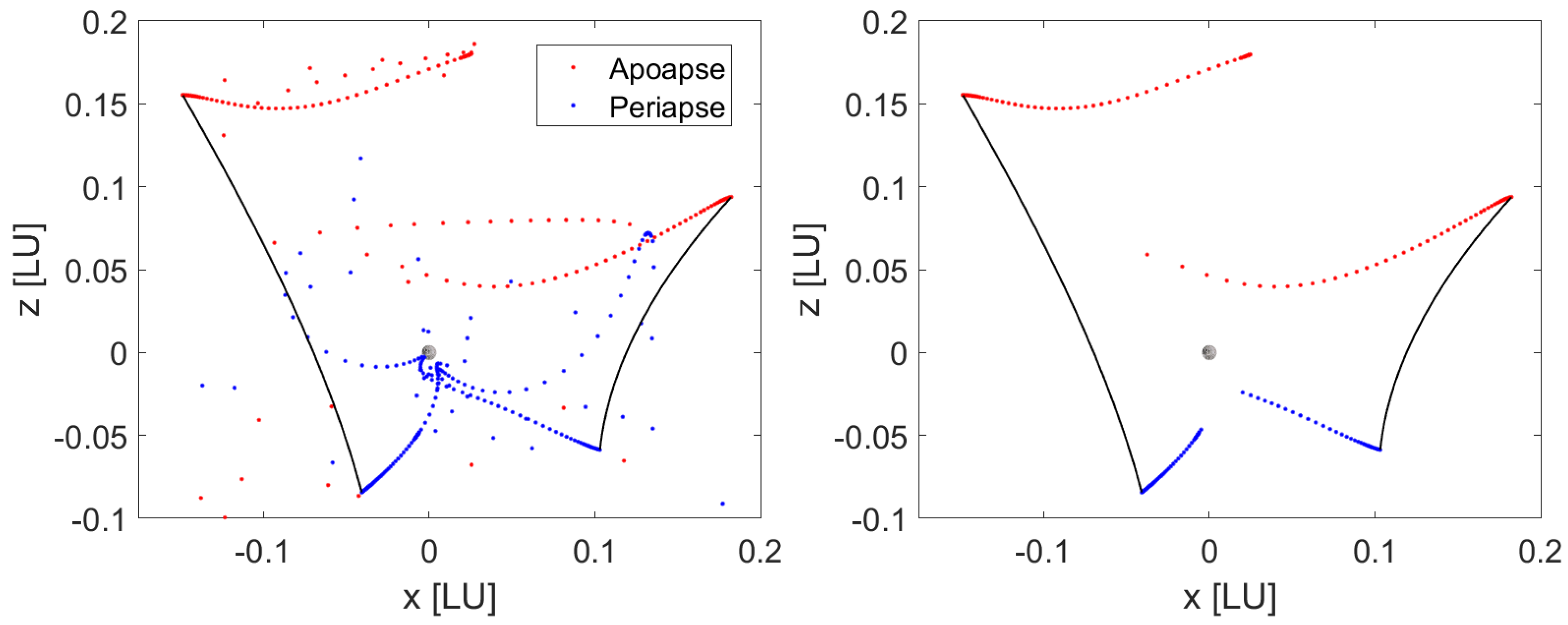
2.5.3. Osculating Conditions

When looking at the restricted “Moon–spacecraft” two-body problem, fuel-efficient transfers tend to gravitate towards periapse and apoapse locations as boundary conditions. Keeping this in mind, a heuristic hypothesis can be proposed wherein these conditions replicate the behavior in higher-fidelity models. Ideally, periapse to apoapse transfers are best suited, but for more complex dynamics, a comprehensive analysis requires quantification of trajectory parameters for all possible combinations.

With an unbounded search space, an infinite number of candidate boundary conditions satisfying the vanishing radial velocity criteria could be obtained. Figure 5 shows this phenomenon, as their location becomes unpredictable and erratic. To avoid the inclusion of said osculating conditions that lie in a close variety of the periodic orbits, the search space was bounded accordingly. These results are also presented within the same figure but are now suitable for continuation.

2.6. Numerical Continuation

Finding solutions for a non-linear system can be challenging, especially if the convergence domain does not permit large deviations from the solution during initialization. If a local solution to a neighboring TPBVP is known, rather than using a randomly initialized “cold start” every time, the similarity dictates a “warm start” by initializing with the known solution. Such a process is called a predictor-corrector scheme, whereby an initial estimate of the solution is made based on previously converged solutions and subsequently corrected to solve for the current states. These so-called continuation methods have previously achieved convergence for low-thrust spacecraft trajectory design applications [11,35]. One straightforward continuation scheme used to aid convergence is natural parameter continuation. By defining a fixed step size of the naturally occurring variable to inform the guess for the unknowns, similar transfer trajectories can be bundled together, allowing for quick and effective convergence and dense mapping of the solution space. Natural parameter continuation, however, cannot track artifacts like turning points/bifurcations in the solution space. It is noted that layering multiple continuation schemes in a nested fashion can further alleviate challenges with convergence.

3. Problem Formulation

In the context of transfers between LPOs, “optimal” transfers can be classified as (1) end-to-end or (2) piecewise. Since there are many scientific applications for deploying spacecraft in cis-lunar space, it is imperative to study and quantify the trade-offs over a dense solution space. The filtered boundary conditions in conjunction with a two-tiered continuation and multi-shooting approach are utilized to map the solution space for transfer trajectories with terminal coast arcs (asymptotic manifolds) connected through a time-optimal intermediate leg. Results are shown for a chosen pair of $L_1$–$L_2$ LPOs, but the presented methodology is generally applicable in any CR3BP system and any periodic orbit pair.

Referring to Figure 6 for a time-optimal transfer architecture, the spacecraft is expected to depart the initial $L_1$ LPO at a prescribed location. The direction of travel is such that the unstable manifold winds off towards the secondary. After a certain time, the low-thrust engine is turned on, providing momentum changes such that the spacecraft deviates from the initial asymptotic trajectory and rendezvous with a prescribed location on the stable manifold of the $L_2$ LPO. Due to the engine being low thrust, judicious utilization of close approaches of the Moon is paramount to complete this transfer. Upon insertion into this trajectory, the manifold will allow it to reach the target periodic orbit. In the subsequent sections, indirect formulation of the time-optimal trajectories and the two-tiered continuation used to map the complete solution space for “COAST-THRUST-COAST” type transfers are discussed in more detail.

3.1. Time-Optimal Trajectories

Time-optimal trajectories aim to minimize the transfer time for the spacecraft. This means that the time of flight is treated as an unknown and must be guessed to solve for an optimal trajectory. These trajectories can be defined either as a “free-insertion” problem, where the insertion point in the target orbit is not important, or as a “rendezvous” problem, where the insertion location is also important and explicitly specified as a boundary condition. In the context of finding the optimal control profile for a trajectory that is time optimal or minimum time, the performance index can be described as $\overline{J}=t_f$, and the Hamiltonian as $\mathrm{H}={\Lambda }^T\dot{\mathbb{X}}$, $\Lambda ={\left[{\lambda }_{\mathbf{X}}{\lambda }_m\right]}^T$ and $\mathbb{X}={\left[\mathbf{X}m\right]}^T$. Utilizing Pontryagin’s minimum principle and primer vector theory to find the optimal control, the TPBVP in the CR3BP is posed as:

$$\mathrm{TPBVP}-\mathrm{Time}-\mathrm{Optimal}\left\{\begin{array}{cc}\hfill & \mathrm{State}\mathrm{Equations}\left\{\begin{array}{cc}\hfill \dot{\mathbf{X}}& =\mathbf{f}+{\displaystyle \frac{T_n{\widehat{\delta }}_t}{m}}\sigma ,T_n=\left({\displaystyle \frac{T}{MU}}\right){\displaystyle \frac{TU}{VU}}\hfill \\ \hfill \dot{m}& =-{\displaystyle \frac{T_n}{c_n}}\sigma ,c_n=I_{sp}{g}_0/VU\hfill \end{array}\right\}\hfill \\ \hfill & \mathrm{Co}-\mathrm{state}\mathrm{Equations}{\dot{\Lambda }}^T=-{\displaystyle \frac{\partial \mathbf{H}}{\partial \mathbb{X}}}\hfill \\ \hfill & \mathrm{Optimal}\mathrm{Control}\left\{\begin{array}{cc}\hfill \sigma & =1\hfill \\ \hfill {\widehat{\delta }}_t& =-{\displaystyle \frac{{\lambda }_{\mathbf{v}}}{|{\lambda }_{\mathbf{v}}{|}_2}}\hfill \end{array}\right\}\hfill \\ \hfill & \mathrm{Boundary}\mathrm{Conditions}\left\{\begin{array}{cc}\hfill \mathbb{X}\left(t_0\right)={\mathbb{X}}_0& ,\mathbf{X}\left(t_f\right)={\mathbf{X}}_f\hfill \\ \hfill \left|\right|{\lambda }_{\mathbf{X}}\left(t_f\right){\left|\right|}_2=1& ,{\lambda }_m\left(t_f\right)=0\hfill \end{array}\right\}\hfill \end{array}\right.$$

(12)

where $\dot{\mathbf{X}}=\mathbf{f}$ denotes the CR3BP dynamics, and $\mathbf{u}$ = ${[\sigma ,{\widehat{\delta }}_t]}^T$ denotes the control inputs, namely throttle and thruster pointing direction, respectively. The primer vector exclusively uses the velocity co-states such that they form a unit vector heading. Note that the formulation above incorporates normalization within the CR3BP continuous-thrust dynamics. These include the spacecraft’s initial mass as the mass unit $\left(MU\right)$ in kg and velocity unit $\left(VU\right)$ as $LU/TU$ given in $\mathrm{k}\mathrm{m}/\mathrm{s}$, whereas the length unit $\left(LU\right)$ and time unit $\left(TU\right)$ are found from the semi-major axis and duration of 1 radian, respectively. The normalized mass, m, is used to determine the current spacecraft mass ratio. At the start, $m\left(t_0\right)=1$, and it diminishes as propellant is used. The normalized thrust $\left(T_n\right)$ and normalized effective exhaust velocity $\left(c_n\right)$ are also used to pose the entire problem in canonical units.

As stated earlier, the thruster operates in full-throttle mode for time-optimal transfers. This is heuristically sensible since the objective is to minimize flight time. Depending on the number of segments, N, the set of unknowns ($S\in {\mathbb{R}}^{14\times (N+1)}$) must be solved for a continuous and valid solution. For the multi-shooting scheme employed in this work, a “free-free” formulation is utilized. At the final state, the respective transversality conditions associated with the unknown parameters (time and mass) must be satisfied along with the continuity conditions at the intermediate times $(t_i,i=1,2,\cdots ,(N-1))$ and terminal state conditions. Typically, the $14\times (N+1)$ unknowns are guessed, and a comprehensive residual function is minimized via a non-linear solver, resulting in a locally optimal solution.

3.2. Manifold Transfer Trajectories

The stable and unstable manifolds of the periodic orbits generate continuous surfaces where the piercing points shown in Figure 4 are locally similar. This allows for a nominal continuation scheme to be implemented that would reduce the computational cost necessary to find all possible permutations and eventually map the dense solution space. The natural parameter in this instance is defined by manifold trajectories within the bundle. Since none of the solutions are known when initializing, a “cold start” must be implemented until an initial convergence is achieved. Subsequently, each successive TPBVP can be “warm started” with the previously converged states. This allows for rapid and efficient convergence, reducing total computational overhead and ensuring convergence over a larger solution space.

Since the problem at hand deals with $L_1$ and $L_2$ LPO transfers (i.e., in the secondary’s vicinity), any non-linear solver will struggle with convergence without an adequate frame transformation of the traditional CR3BP synodic frame due to increased sensitivities. Therefore, the problem was posed in a selenocentric rotating frame rather than the original barycentric frame. The dynamical system described by Equations (1), (2) and (12) is transformed via the following equation: $\tilde{x}=x-1+\mu$. The co-state dynamics are re-derived to reflect the selenocentric frame. For this paper, MATLAB’s mex version of ode45 was implemented to propagate the state–co-state dynamics with relative and absolute tolerances of ${10}^{-12}$. The entire TPBVP required fsolve of 100,000 maximum iterations and function evaluations, of which the step and function tolerances were maintained at ${10}^{-12}$. The overall scheme can be summarized as follows (Algorithm 1):

Algorithm 1: Two-Tiered Continuation Algorithm

Note that the problem is initially solved using a single segment multi-shooting scheme to leverage the free-free boundary conditions for continuation, but these values are re-converged in the final step. When re-converging, the fixed-free single shooting method is used with the same tolerances, this reduction in the overall search variables reduces both computational and compounding errors. Over the entire solution domain, the spacecraft’s final mass is then used to estimate the $\Delta v$ costs for the respective stable-unstable manifold pairs using the “coast-thrust-coast” control profile which varies the manifold coast states. Likewise, the cumulative time-of-flight can be computed via a summation of the time spent throughout all the legs of the trip.

4. Results

Using the described problem formulation and solution methodology, two Earth–Moon northern halo orbits were selected as a use case for determining the piece-wise optimal transfers leveraging invariant manifold pairs as terminal coast segments. For establishing a control group, direct time-optimal transfers were performed on the ${\mathrm{EML}}_1$ and ${\mathrm{EML}}_2$ periodic orbit pair with Jacobi constants 3.0326 and 3.1166, respectively [38]. Before analyzing the fuel savings and the commensurate trade-offs with transfer time, direct transfers are solved by discretizing the two periodic orbits to set up the end-to-end transfer problem. The results below are for a spacecraft equipped with a low-thrust engine with an $I_{sp}$ of 4170 s (similar to one of NASA’s NEXT engine operating modes [40]). While the final results use $1\times {10}^{-3}$ m/${\mathrm{s}}^2$ as the thrust acceleration, to provide a comprehensive perspective on this class of transfer trajectories, some results are also presented for higher thrust accelerations—$2\times {10}^{-2}$ m/${\mathrm{s}}^2$, $1\times {10}^{-2}$ m/${\mathrm{s}}^2$, and $5\times {10}^{-3}$ m/${\mathrm{s}}^2$—in the following section.

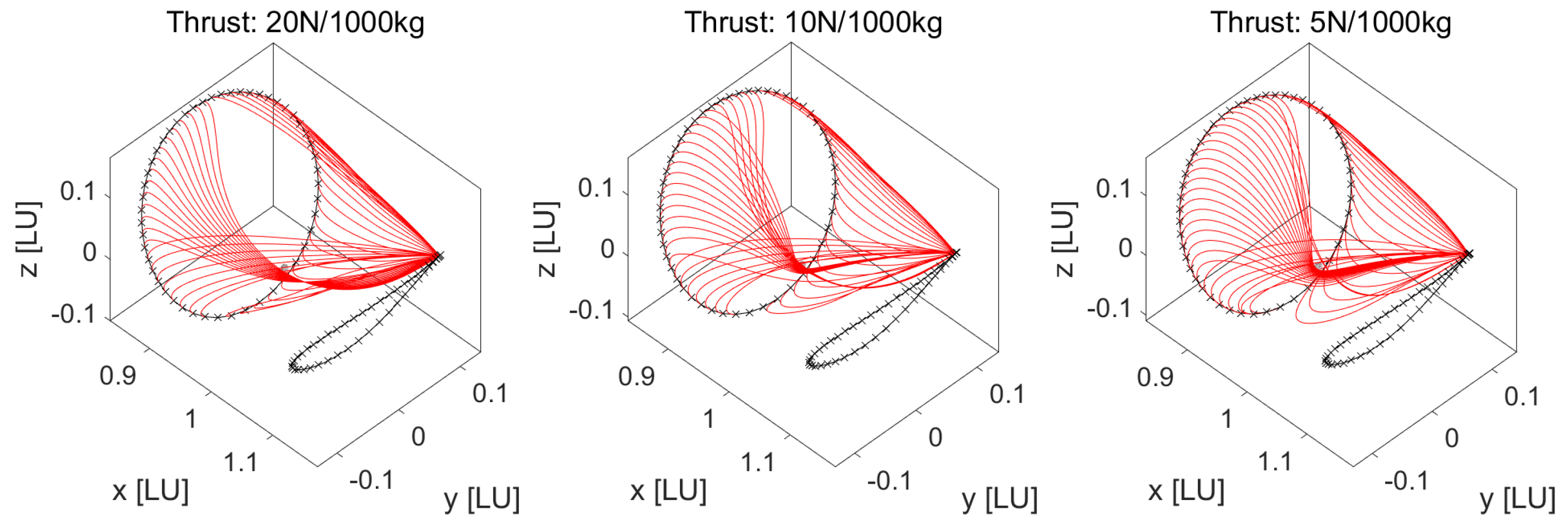
4.1. Direct Transfers

The quickest transfer between the two orbits given a bounded control can be determined by solving an end-to-end time-optimal transfer for all combinations of discretized states on the two orbits and picking the “global” minima. The straightforwardness of such a maneuver means that the time will be minimized at the expense of higher total fuel consumption. Nevertheless, by solving this problem, the relative fuel savings for manifold-assisted transfers can be contextualized. It is apparent that if the periodic orbits are discretized into N fixed points, the total number of TPBVPs is $N^2$, which includes all combinations of terminal states. For the current analysis, $N=50$; therefore, 2500 TPBVPs were solved to reveal the optimal control profile associated with each transfer.

Upon performing a qualitative analysis for decreasing thrust acceleration levels, Figure 7 shows that for the same TPBVP, the trajectory profiles are remarkably different. This is due to the relative values of the instantaneous thrust acceleration and the lunar perturbation. With a stronger control authority, the lunar gravity well can be traversed through ‘brute force’ with minimal alteration. It was also observed that for the lowest thrust acceleration analyzed as a part of this work (see Figure 8), a cyclical pattern emerges in fuel consumption with well-pronounced regions of optimality. This can be attributed to certain boundary conditions, enabling the spacecraft to leverage the close lunar encounters rather than fighting off the lunar gravity well.

The transfer requiring the least fuel consumption is depicted in Figure 9 and validates the discussed qualitative insights. This trajectory has a close encounter with the Moon and leverages the momentum change due to the underlying physics of the system. Quantitatively, the most fuel-efficient transfer required a $\Delta$V = 566 m/s, amounting to $13.74$ kg for every 1000 kg onboard, before executing the burn. From start to finish, the total time of flight was 6.5 days for the described end-to-end transfer.

These qualitative metrics provide a benchmark to compare the trade-offs by using manifolds to assist such transfers. The relative position indicates the time to reach that state from the topmost point on the periodic orbit, normalized by the time period. Since the optimal case had an initial position of 0.24$T_1$, starting from the state with the maximum $z-amplitude$, a forward propagation is performed to 0.24 periods or 0.652 $TU$, as the period is 2.717 $TU$. The same process is repeated for the ending terminal at 0.92$T_2$, except that the orbital period is now 3.339 $TU$ for that LPO. If the value is negative, then the system is back-propagated to find the states.

4.2. Manifold-Assisted Transfers—Plane Piercings

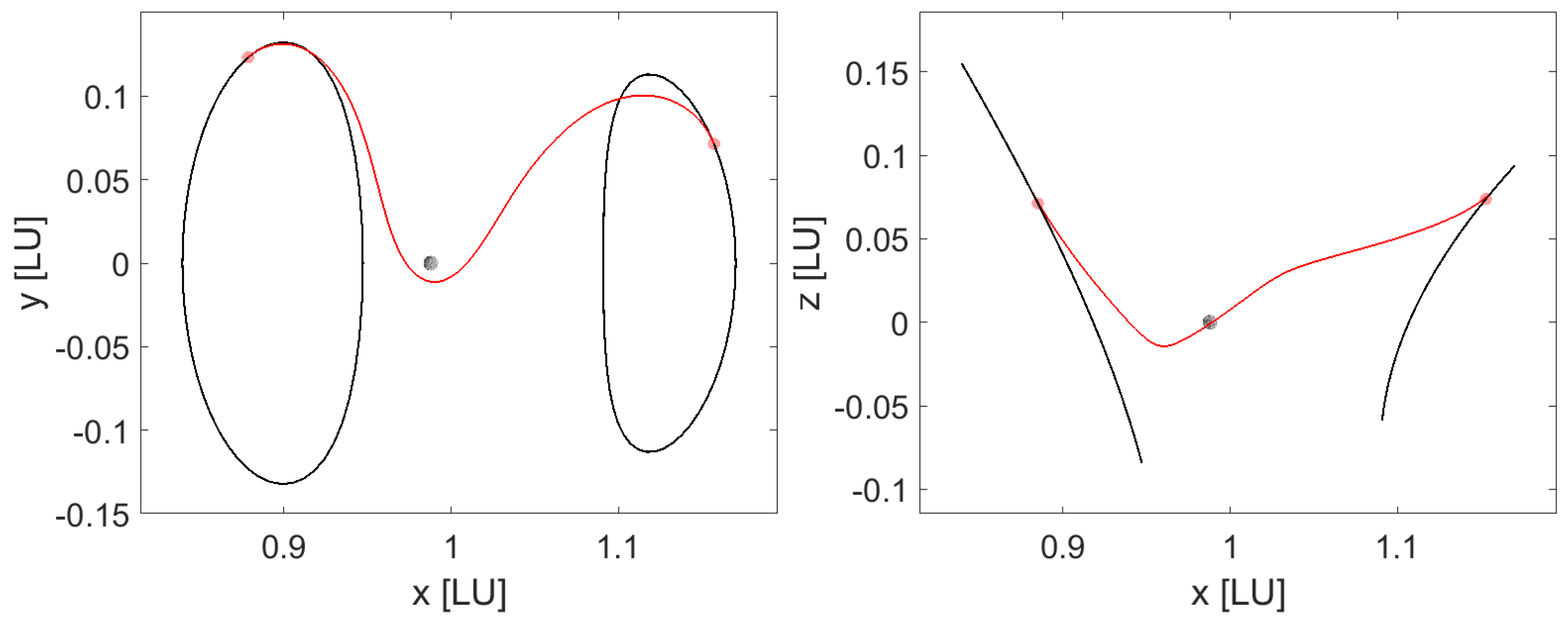
This section presents results for manifold-assisted transfers utilizing plane-piercing way-points. It was observed that for the acceleration levels that are commensurate with low-thrust propulsion, convergence for boundary pairs was extremely challenging. The reason for this comes from the geometric dissimilarity in the target states associated with the plane-piercing conditions, rendering the problem numerically intractable in most cases. Additionally, for the sparse regions in the solution space where convergence was possible, significant bifurcations were observed, which contributed to further challenges in performing continuation.

Figure 10 shows an example of bifurcation in locally optimal solutions where the result shows markedly different “time-optimal” intermediate legs between identical boundary conditions. The converged trajectory depicted in the left sub-image has a longer flight time and therefore higher fuel costs but still satisfies the first-order optimality conditions, which is the same as the solution on the right. Nevertheless, in both cases, the spacecraft has a close lunar encounter, passing through an osculating periapse condition, which alters the trajectory significantly, as expected. This is heuristically characteristic of time-optimal solutions as the relative time traveled reduces near periapsis conditions and the Moon assists in orbital alterations. Nonetheless, a sphere is more emblematic of the dominant lunar gravity in the vicinity of the Moon. Therefore, using a “fictitious” sphere of influence to filter boundary conditions is anticipated to lead to geometrically consistent mathematical formulations.

4.3. Manifold-Assisted Transfers—Sphere Piercings

Now that a sphere defines the piercing surface, this boundary set acts as a pseudo-sphere of influence (pseudo-SOI). A thrust variation study shows how the continuous-thrust pathways are still significantly altered by the lunar gravity well.

Figure 11 shows that for high-thrust acceleration, the trajectory stays within the confines of the sphere, the radius of which was 34,760 km or ≈20 times the equatorial lunar radius ($20{\mathrm{R}}_{\mathrm{m}}$). For lower thrust levels, it was observed that the spacecraft exits the sphere to transfer between manifold states. This effect is more pronounced than direct transfer due to the constrained filtering of boundary conditions. Although this seems drastic, the typical cost is much lower as travel time is much shorter between the manifold states.

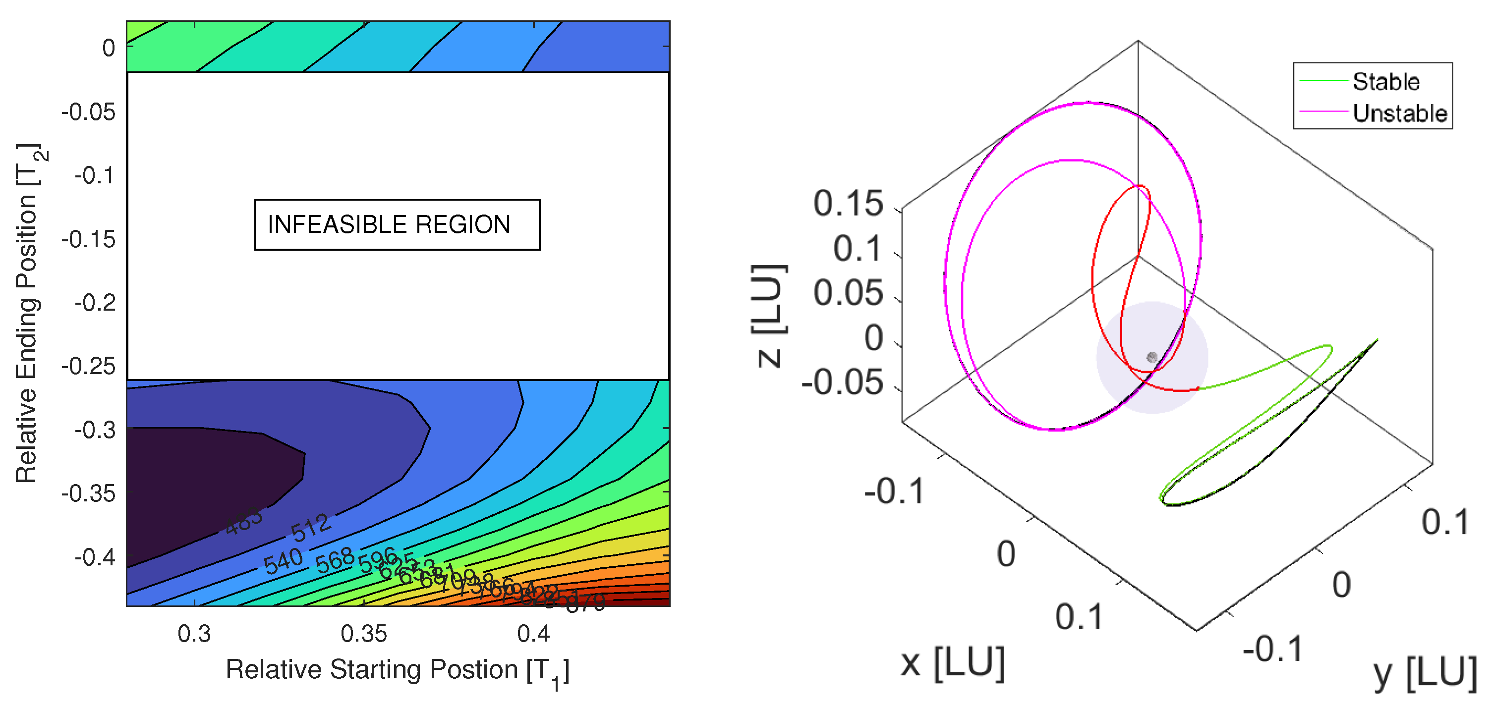
To capture any interplay between sub-optimality and ballistic descent into the lunar gravity well, the pseudo-SOI was reduced up to $\approx 10{\mathrm{R}}_{\mathrm{m}}$ and the two-tiered continuation scheme was employed to densely map the solution space. Solution sets for sphere sizes of 18, 14, and 10 ${\mathrm{R}}_{\mathrm{m}}$ are shown in Figure 12, where, as the radius decreases in size, constrained filtering results in a sparse boundary condition set. Ergo, the solution space shrinks, and numerical convergence becomes more challenging. As seen from Figure 13, pork chop plots depict distinct regions of fuel-optimality. Note that vacant regions denote sub-domains where convergence was not achieved. Further analysis revealed that such cases include trajectories with extremely close/catastrophic encounters with the Moon. Leveraging the underlying physics is beneficial, and the solver attempts to secure optimality to the detriment of crashing the spacecraft. The dark blue region depicts optimal solutions that briefly pass by the Moon but do not crash. The most fuel-efficient solution required a $\Delta$V = 463 m/s, or $11.26$ kg for every 1000 kg of the initial mass. The geometry of the optimal transfer shows the spacecraft has two lunar encounters: the first to escape the gravitational well and change direction, and the second to rendezvous with the stable manifold. Using linearized correlation analysis to study the interdependence of the change in selenocentric orbital elements at the boundary conditions, specifically eccentricity and inclination $\{\Delta e,\Delta i\}$ with $\Delta$V, the linear correlation between $\{\Delta \mathrm{V},\Delta e\}$ was statistically similar, ≈0.09.

Continuing onto 14 ${\mathrm{R}}_{\mathrm{m}}$, the domain of boundary-condition combinations shrinks as more regions become inaccessible. However, the overall contours in Figure 14 still bear a significant resemblance to the 18 ${\mathrm{R}}_{\mathrm{m}}$ solution space. The most fuel-efficient case also shows similar qualitative and quantitative characteristics, requiring a $\Delta$V = 448 m/s, or $10.89$ kg for every 1000 kg of the initial mass. The linear correlation between $\{\Delta \mathrm{V},\Delta e\}$ was statistically stronger, growing to ≈$0.42$. Based on the observed trends, further reduction in sphere size would be expected to lead to increased fuel savings. However, this was not observed upon mapping the 10 ${\mathrm{R}}_{\mathrm{m}}$ solution space. The increased lunar proximity of the boundary conditions made the initial “cold starts” ineffective, and therefore a continuation path was required. As depicted on the pork chop plot, there is an increase in area of the vacant regions. The most fuel-efficient solution required a $\Delta$V = 455 m/s, or $11.06$ kg for every 1000 kg of the initial mass. The linear correlation trends were consistent, and $\{\Delta \mathrm{V},\Delta e\}$ bore a stronger correlation, slightly less pronounced than the previous case, ≈0.28, indicating a relation between the boundary condition set and optimality.

Table 1. Linear correlation coefficients for time-optimal solution sets sorted by SOI radius.

Radius (${\mathit{R}}_{\mathit{m}}$)	${\mathit{C}}_{\mathbf{\Delta }\mathit{v},\mathbf{\Delta }\mathit{e}}$	${\mathit{C}}_{\mathbf{\Delta }\mathit{v},\mathbf{\Delta }\mathit{i}}$
20	$0.06$	$0.03$
18	$0.09$	$0.08$
16	$0.26$	$0.16$
14	$0.42$	$0.19$
12	$0.36$	$0.10$
10	$0.28$	$0.07$

denotes the linearized correlation coefficients for six discrete sphere sizes, $10{\mathrm{R}}_{\mathrm{m}}\le R\le 20{\mathrm{R}}_{\mathrm{m}}$. Generally, the dependence of $\Delta$V on changes in osculating seleno-centric orbital elements, particularly eccentricity and inclination osculating conditions, at larger distances from the Moon is minimal due to the physical significance of the sphere of influence. As the sphere radius is reduced, the interdependence grows stronger until the solution domain shrinks substantially and the vacant sub-domains grow. The eccentricity change is by far the most significantly correlated with fuel cost, and it is found upon further analysis that fuel-efficient maneuvers typically have the lowest $\Delta e$ values. Most of the time, these boundary conditions denote elliptical selenocentric orbits that are near-parabolic. The inclination does not truly affect the fuel costs, only in that the direction of motion may indicate the relative stability of the orbit in the three-body problem. Normally, naturally occurring prograde orbits are much more unstable than naturally occurring retrograde ones within the CR3BP; ergo, leveraging the natural instability translates to more economical maneuverability.

When looking specifically at the most fuel-efficient case for each sphere size, it is clear that the lowest possible fuel cost is achieved through a judicious close encounter with the Moon. The term ‘judicious’ indicates that lunar gravity should be leveraged just enough to facilitate the transfer, but descending deeper into the gravity well is detrimental. The solutions listed in

Table 2. “Global” piecewise-optimal, manifold-assisted transfers sorted by SOI radius.

Radius (${\mathit{R}}_{\mathit{m}}$)	${\mathit{T}}_1$	${\mathit{T}}_2$	$\mathbf{\Delta }\mathit{v}$ (m/s)	$\mathbf{\Delta }\mathit{a}$ (LU)	$\mathbf{\Delta }\mathit{e}$	$\mathbf{\Delta }\mathit{i}$ (°)	t (TU)
20	$0.28$	$0.68$	476	$0.06323$	$-0.0244$	$30.91$	$15.47$
18	$0.20$	$0.64$	463	$0.06088$	$0.0359$	$37.94$	$15.57$
16	$0.22$	$0.64$	455	$0.06476$	$0.0641$	$46.96$	$15.57$
14	$0.22$	$0.62$	448	$0.06778$	$0.1325$	$56.7$	$15.60$
12	$0.26$	$0.64$	451	$0.07116$	$0.1121$	$60.5$	$15.59$
10	$0.28$	$0.64$	455	$0.07348$	$0.1297$	$63.6$	$15.62$

have similar initial and final configurations. These manifold pairs have the unique characteristic of a small discrepancy in eccentricity and inclination changes within a small bounded region around ${50}^{\circ }$. Although this seems drastic, both the thruster and the Earth’s presence cause greater momentum changes at locations farther from the Moon, which explains this discrepancy. As shown in Figure 13, Figure 14 and Figure 15, the inclination change that optimal solutions tend towards is ≈${50}^{\circ }$ as a byproduct of the previously discussed relationship. The total flight time is consistent even with different sphere sizes, where the values range from 68–70 days from start to finish. This value is much greater than the direct transfer solution of 6.5 days but results in fuel savings of up to 20%, which is significant.

4.4. Manifold-Assisted Transfers—Osculating Conditions

To test the hypothesis that filtering via restricted two-body osculating periapsis and apoapsis condition may lead to more fuel-efficient transfers, further analysis was conducted using the same LPO pair. Usable perilune and apolune conditions were determined by forward propagating the manifolds upon departing the periodic orbit’s neighborhood. Otherwise, the proximity of the osculating points to the original orbit would diminish the coast segments and mimic direct transfers in the limiting case.

Figure 16 depicts the solution bundles graphically, with each solution family exhibiting starkly different characteristics. In the conditions starting at apolune, the spacecraft is far enough from the Moon that maneuvering is straightforward. If the lunar gravity well is used, then the fuel spent is expected to be minimized. Nevertheless, since the distance traveled is much longer, the overall costs are significantly higher than those from the sphere-piercing sets. When targeting perilune, most solutions must turn around to enter the stable manifold conditions, thus leading to long journey times as this is performed far from the Moon. For the most efficient solution, though, the boundary pairs are similar enough that only a small powered segment is necessary. The perilune initial states meant that the spacecraft has already performed the flyby and therefore could not leverage it to diminish fuel costs. This is why, for cases starting at perilune, the powered segment took the spacecraft away from the Moon rather than towards it. Many of these solutions are actually mimicking hetero-clinic connections where none are present. Ergo, for the rest of the cases aside from apolune to apolune, the primary indicator for fuel cost was the dissimilarity of the initial and final states. This is also reflected in the most fuel-efficient transfer in each “class”, as shown in

Table 3. “Global” piecewise-optimal, manifold-assisted transfers sorted by osculating pairs.

Direction	${\mathit{T}}_1$	${\mathit{T}}_2$	$\mathbf{\Delta }\mathit{v}$ (m/s)	$\mathbf{\Delta }\mathit{a}$ (LU)	$\mathbf{\Delta }\mathit{e}$	$\mathbf{\Delta }\mathit{i}$ (°)	t (TU)
A-A	$0.79$	$0.30$	593	$0.0571$	$-0.477$	$-17.0$	$14.12$
A-P	$0.92$	$0.15$	488	$0.0260$	$0.3414$	$45.8$	$14.55$
P-A	$0.05$	$0.88$	472	$0.0609$	$-0.243$	$-15.7$	$14.19$
P-P	$0.96$	$0.32$	548	$0.0666$	$0.4038$	$34.5$	$14.37$

. Figure 17 then compares the most fuel-efficient solutions across all filtering techniques analyzed in this work.

It must be noted that computational cost must also be considered to evaluate efficacy, as the boundary conditions and engine parameters may significantly alter convergence time. The total time for completion varied with each scheme due to a multitude of factors but averaged ≈ 2 s for each TPBVP. However, the computational time was severely correlated with boundary conditions. Sometimes, up to 10 solutions were found each second using continuation since the trajectories were geometrically similar, and convergence was achieved in a few hundred iterations. In certain regions of the solution space, numerical convergence was either not achieved or required a large number of iterations. For such cases, it may prove valuable to use cold-starts. Luckily, most cases were well behaved and converged rapidly towards a solution. This indicates the computational advantages of the two-tiered continuation technique. In future work, rather than employing grid search, gradient-based approaches could improve computational cost.

After analyzing direct transfers, plane-piercing, and sphere-piercing boundary conditions for time-optimal solutions, it was shown that low-thrust transfers using terminal ballistic arcs as coast segments can unearth a dense solution space, which can be leveraged for designing transfers between LPOs centered around the Moon. Better solutions appeared when the constraint conditions were set to those of sphere-piercing points more so than any other as they better resembled the periodic orbit geometries.

5. Conclusions

Searching for low-thrust direct transfers between LPOs is rife with numerical challenges due to the small, continual change in momentum being insufficient to overcome the gravitational forces experienced while transitioning through the lunar vicinity. Future endeavors to support sustained cis-lunar presence will have mission architectures that are far more dynamic and require rigorous transfer designs. This paper presented a systematic approach to densely map the manifold-assisted trajectories with an intermediate-powered leg. Rather than using a strictly fuel-optimal approach, a time-optimal manifold-assisted transfer was implemented to indicate the magnitude of expected fuel costs, and key design trade-offs were quantified. A two-tiered continuation scheme determined the time-optimal solution space for direct transfers between the two periodic orbits. Continuation was specifically selected to warm start the shooting scheme rather than cold start it, which drastically sped up the process. It was demonstrated that with decreasing maximum thrust, the spacecraft either had to leverage the lunar gravity to change course or move far enough away that the engines, with the assistance of the Earth, would be able to maneuver efficiently.

To circumvent the boundary condition filtering challenges on the manifold trajectories, plane-piercing, sphere-piercing, and osculating periapsis/apoapsis mapping approaches were studied. Issues arose when solving for the planar conditions as multiple larger discontinuities were prevalent. This often led to unsuccessful convergence attempts, inefficient maneuvers, or solution bifurcations. The sphere intersections proved to be more robust. Additionally, the popular approach of using discrete osculating periapsis conditions defined by a restricted two-body problem in the lunar vicinity to quantify transfer costs was also studied. This process demonstrated that an osculating periapsis to periapsis transfer is not the optimum choice universally. It was further observed that with a reduction in the pseudo-SOI radius, the design domain shrunk. Analysis of the corresponding selenocentric osculating orbital elements for the “global optimal” solution revealed that the osculating eccentricity change was minimal. Another key insight was that the prograde trajectories tended to be far more maneuverable due to their general inherent instability in the CR3BP.

The most fuel-efficient solution based on the restricted domain and control profile occurred at ≈12 ${\mathrm{R}}_{\mathrm{m}}$, requiring $\Delta \mathrm{V}=448$ m/s be used, a savings of 20% when compared to the analogous optimal end-to-end transfer at the expense of an increase in transfer time by 61–64 days. The underlying methodology presented is general in applicability across different primary–secondary pairs and lower thrust acceleration levels. The selected case study is of importance to future cis-lunar efforts and instills confidence in leveraging a manifold-assisted transfer approach to find fuel-efficient solutions through a densely populated design space and improved numerical convergence.