Model-Free Adaptive Control for Attitude Stabilization of Earth-Pointing Spacecraft Using Magnetorquers

Abstract

This paper presents an attitude stabilization algorithm for a Low Earth Orbit (LEO) Earth-pointing spacecraft using magnetorquers as the only torque actuators and employing Model-Free Adaptive Control (MFAC) as the control algorithm. MFAC is a data-driven control algorithm that relies solely on input–output data from the plant. This paper validates the effectiveness of the proposed approach through numerical simulations in a specific case study. The simulations show that the proposed algorithm drives the spacecraft’s attitude to three-axis stabilization in the orbital frame from arbitrary initial tumbling conditions. The numerical study also shows that the proposed control algorithm outperforms a model-based Proportional–Derivative (PD) control in terms of pointing accuracy at the expense of higher energy consumption.

1. Introduction

Spacecraft often have an attitude stabilization system. They can be either passive (e.g., spin-stabilized or gravity gradient-stabilized systems [1]) or active. The most accurate active stabilization systems usually include momentum or reaction wheels. However, in some spacecraft flying in low Earth orbits, attitude stabilization is achieved using magnetorquers. These systems are composed of flat coils, which are activated by electric currents and securely positioned on the spacecraft, usually along three perpendicular axes. They function by utilizing the interaction between the magnetic dipole moment produced by these coils and the Earth’s magnetic field. Specifically, this interaction with the Earth’s field induces a torque that endeavors to orient the entire magnetic dipole moment in alignment with the direction of the field. Consequently, magnetorquers present the following strong points: (i) they offer simplicity, reliability, and affordability; (ii) they solely require renewable electrical power for their operation; (iii) they contribute to reducing overall system weight when compared to alternative torque actuators. However, magnetorquers come with significant drawbacks: (i) the control torque they produce is limited to the plane perpendicular to the Earth’s magnetic field; (ii) their maximum torque output is considerably lower compared to other types of torque actuators. As a result of these limitations, relying exclusively on magnetorquers for attitude control results in reduced pointing accuracy and slower convergence in comparison to alternative torque actuators [2]. Attitude stabilization through magnetorquers has been explored as a viable choice, particularly for cost-effective micro- and nanosatellites and satellites encountering failures in their primary torque actuators [3]. Paper [4] provides an extensive review of results on several methods for active attitude control using magnetic actuators.

This paper focuses on active three-axis attitude stabilization of an Earth-pointing spacecraft with magnetorquers as the only torque actuators and without onboard momentum storage. The literature in this specific area of research is vast, and several works propose PD-like stabilization laws. Since a spacecraft with magnetometers is intrinsically a time-varying plant due to the variation in the geomagnetic field along the orbit, selecting the PD gains is not a straightforward task. In [5], the scalar PD gains are selected to guarantee stability by considering the locus for the characteristic multipliers. Reference [6] presents a semi-analytic approach for selecting scalar gains that optimize the time response. Paper [7] proposes time-varying matrix gains that guarantee stability by solving linear–quadratic optimization problems. The same work also presents a method for designing constant matrix gains considering a time-invariant approximated model. However, the method does not guarantee stability, which must be checked separately. Work [8] also determines time-varying gains by a linear–quadratic approach and extends it to the rejection of generic disturbance torques. A similar approach in discrete time is employed in [9]. In [10,11], constant matrix gains are designed by solving a different linear–quadratic optimization problem by which stability is obtained. Paper [12] proposes an adaptation mechanism for the gains to guarantee stability and also convergence to the nominal attitude for almost all initial conditions. A different PD-like stabilization law is presented in [13], where the gains are determined through a heuristic optimization strategy without providing an analytical stability analysis. A reconfiguration method for a PD-like stabilization law in case of failure of a magnetometer is proposed in [14]. A Proportional–Integral–Derivative (PID)-like stabilization algorithm is employed in [15] to achieve more accurate pointing. However, similarly to before, the proposed method does not guarantee stability, which must be checked after having determined the gains. Reference [16] proposes a more complex law designed by a robust backstepping method which achieves global asymptotic stability. Work [17] presents a two-timescale control in which, first, the pitch axis is aligned to the orbit normal, and then the pitch rate is enforced to the desired value, thus achieving stability for the closed loop. Paper [18] presents an algorithm based on a sequence of Riccati equations for which stability is not guaranteed.

All the designs presented in the cited works present limitations in rejecting the effects of some disturbance torques. This is probably a consequence of the fact that those designs are model-based, and models for those disturbance torques are not included in the design process. To overcome the above limitation, data-driven control can be a valid alternative. Indeed, in data-driven control, there is no necessity for a mathematical spacecraft model in the design process. It relies completely on the measurements coming from the Input/Output (I/O) data of the plant that have to be controlled. Data-driven control methods are divided into two main categories: online and offline data-driven methods. In offline methods, controller parameters are estimated through a learning process before implementation on the controlled plant. Several offline data-driven methods have been developed including iterative feedback tuning [19], correlation-based tuning [20], virtual reference feedback tuning [21], and PID control [22]. On the other hand, in online data-driven methods, only initial values are assigned to the controller parameters, which are updated online without employing any identification process. Several online data-driven methods were developed such as Simultaneous Perturbation Stochastic Approximation (SPSA) [23], unfalsified control [24], dynamic neural network-based control [25], and model-free adaptive control [26,27,28].

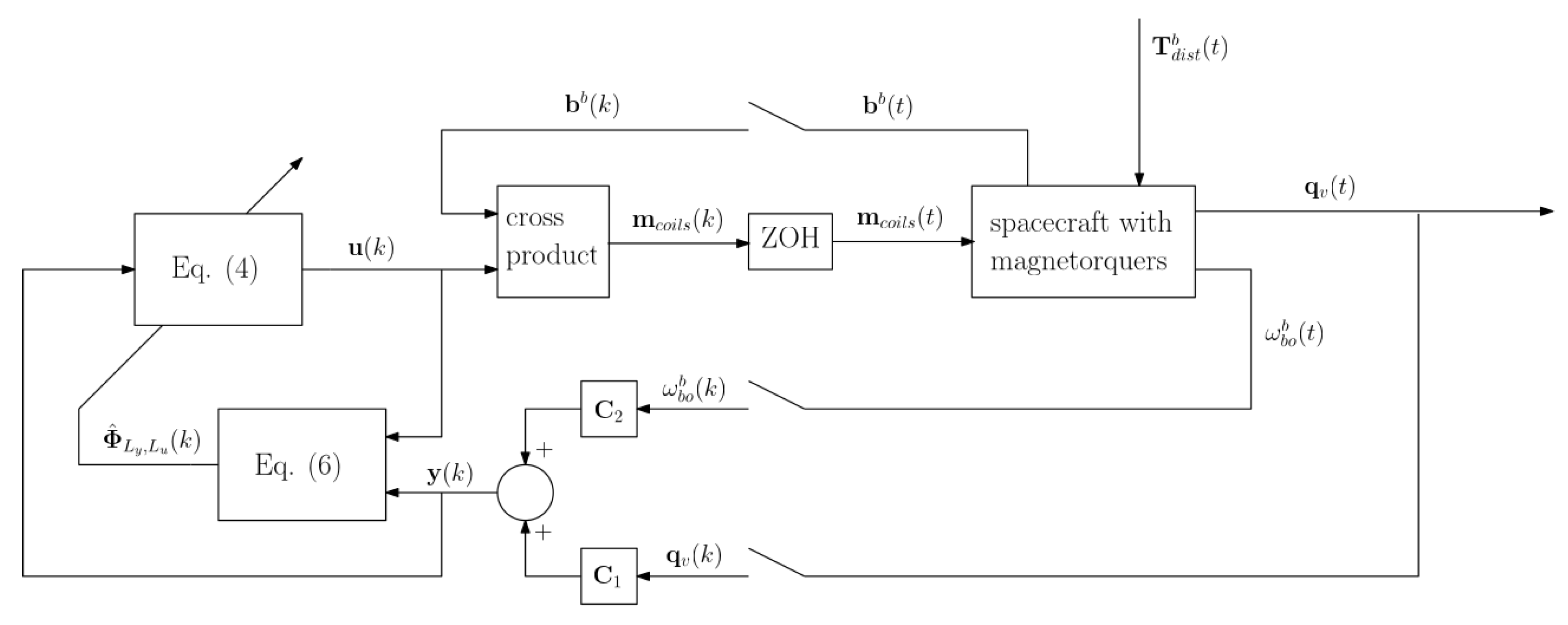
Online data-driven control was employed for three-axis stabilization of an Earth-pointing spacecraft with magnetorquers in [29], in which dynamic neural networks were utilized. In this paper, the same type of attitude stabilization is performed by using a different online data-driven method known as Model-Free Adaptive Control (MFAC). The MFAC method is based on the dynamic linearization technique and a new concept called Pseudo Partitioned Jacobian Matrix (PPJM) [26]. The PPJM is employed to dynamically linearize the nonlinear plant in real time, based on I/O measurement data. By estimating the PPJM, the controller output can be calculated. The MFAC method stands out as a feasible solution for the attitude stabilization of spacecraft with magnetorquers due to the following reasons: (1) no mathematical model of the spacecraft with magnetorquer is required, leading to the design of an attitude controller which is solely based on the available I/O measurement data; (2) when contrasted with other data-driven controllers, MFAC requires the tuning of few parameters and low computational effort, making it a practical and efficient choice; (3) MFAC is known for its adaptive structure, allowing it to handle variations in the spacecraft’s dynamics and environmental conditions; in fact, spacecraft operations can involve different variations such as those due to changing payloads and orbital conditions, and MFAC can adapt control actions based on real-time measurements; (4) some control methods require knowledge of bounds on the plant initial conditions which are unnecessary for MFAC; such a feature is advantageous for spacecraft control, where obtaining those bounds could be unfeasible; (5) MFAC has demonstrated successful implementation in various practical fields such as combustion systems [30], combined spacecraft [31], unmanned surface vehicles [32], launch vehicles [33,34], air vehicle pitch channels [35], moving mass controlled flying robots [36], multiagent systems [37], autonomous cars [38], wastewater treatment processes [39], wind turbine rotors with controllable flaps [40], and satellites with large rotational components [41].

The effectiveness of the MFAC design is evaluated through numerical simulations. Specifically through Monte Carlo campaigns, it is shown that the designed attitude controller is able to achieve three-axis stabilization in the orbital frame from an arbitrary tumbling condition. Moreover, the numerical study also reveals that the proposed control algorithm outperforms a model-based PD control in terms of pointing accuracy at the expense of higher energy consumption.

Employing MFAC for three-axis stabilization of an Earth-pointing spacecraft using only magnetorquers represents a novel approach. In [31], the MFAC method is used for the attitude stabilization of a combined spacecraft that is fully actuated and is not affected by disturbance torques. The main differences compared to the attitude stabilization considered in [31] are as follows: (i) torque actuation is obtained by using magnetorquers in place of reaction flywheels; (ii) disturbance torques are considered in evaluating the performance of the proposed method; (iii) stabilization is performed with respect to the orbital frame instead of an inertial frame. As a result, in all above aspects, the present work presents advancements with respect to [31]. In [41], a modified version of MFAC called model-free prescribed performance adaptive control is employed for the attitude stabilization of a fully actuated satellite with large misaligned rotational components.

This paper is organized into the following sections: The next section describes the attitude of an Earth-pointing spacecraft with magnetorquers. Section 3 introduces the MFAC algorithm employed to stabilize the spacecraft’s attitude. Numerical simulations and evaluation of the obtained results are included in Section 4. Concluding remarks end the paper. The paper includes an appendix which concisely recalls the theoretical framework of MFAC.

2. Attitude of Earth-Pointing Spacecraft with Magnetorquers

2.1. Coordinate Frames

To describe the attitude motion of a rigid Earth-pointing spacecraft in a circular orbit, it is advantageous to introduce reference frames as follows:

• Geocentric Inertial Frame denoted by ${\mathcal{F}}_i$. This frame is commonly used for Earth orbits. It is centered at the Earth’s core. The $x_i$ axis corresponds to the vernal equinox direction, the $z_i$ axis points northward along the Earth’s axis of rotation, and the $y_i$ axis is chosen to create a right-handed coordinate system.
• Orbital frame denoted by ${\mathcal{F}}_o$. This frame is also known as the Local Vertical Local Horizontal (LVLH) frame. The origin of the frame is at the spacecraft’s center of mass. The $x_o$ axis aligns with the spacecraft’s velocity direction, the $z_o$ axis is aligned with the nadir direction, and the $y_o$ axis is oriented perpendicular to the orbital plane, forming a right-handed coordinate system.
• Spacecraft body frame denoted by ${\mathcal{F}}_b$. The origin of the body frame coincides with the spacecraft’s center of mass, and its axes align with principal axes of inertia of the spacecraft.

The desired Earth-pointing orientation corresponds to aligning ${\mathcal{F}}_b$ with ${\mathcal{F}}_o$.

A summary of the notation used in this paper can be found in

Table 1. Notation.

Symbol	Meaning
$\overrightarrow{\mathbf{b}}$	geomagnetic field on spacecraft
n	spacecraft orbital rate
$\mathbf{q}$	quaternion related to attitude of ${\mathcal{F}}_b$ relative to ${\mathcal{F}}_o$
${\mathbf{q}}_v$, $q_4$	vector part and scalar part of quaternion $\mathbf{q}$
${\mathbf{v}}^i$, ${\mathbf{v}}^o$, ${\mathbf{v}}^b$	column matrices of coordinates of vector $\overrightarrow{\mathbf{v}}$ resolved in ${\mathcal{F}}_i$, ${\mathcal{F}}_o$, and ${\mathcal{F}}_b$, respectively
${\mathbf{I}}_{3\times 3}$	three-dimensional identity matrix
${\overrightarrow{\mathit{\omega }}}_{bo}$	angular velocity of ${\mathcal{F}}_b$ relative to ${\mathcal{F}}_o$
${\overrightarrow{\mathit{\omega }}}_{bi}$	angular velocity of ${\mathcal{F}}_b$ relative to ${\mathcal{F}}_i$
${\overrightarrow{\mathit{\omega }}}_{oi}$	angular velocity of ${\mathcal{F}}_o$ relative to ${\mathcal{F}}_i$

.

2.2. Attitude Stabilization Using Magnetorquers

In this work, the primary focus is on the attitude of the spacecraft in relation to the orbital frame. The attitude of ${\mathcal{F}}_b$ relative to ${\mathcal{F}}_o$ is here represented by using quaternion denoted by $\mathbf{q}$ that is indicated as follows:

$$\mathbf{q}={\left[q_1{q}_2{q}_3{q}_4\right]}^T={\left[{\mathbf{q}}_v^T{q}_4\right]}^T$$

with the condition $\parallel \mathbf{q}\parallel =1$. The angular velocity of ${\mathcal{F}}_b$ relative to ${\mathcal{F}}_o$ resolved in ${\mathcal{F}}_b$ is denoted by ${\mathit{\omega }}_{bo}^b$.

The spacecraft employs three magnetic coils as torque actuators that are aligned with the axes of the spacecraft’s body frame ${\mathcal{F}}_b$. These coils generate a magnetic control torque through the following mechanism:

$${\mathbf{T}}_{coils}^b={\mathbf{m}}_{coils}\times {\mathbf{b}}^b$$

(1)

where ${\mathbf{m}}_{coils}$ represents the magnetic dipole moment generated by the three magnetorquers, ${\mathbf{b}}^b$ represents the geomagnetic field at the position of the spacecraft, and both are resolved in ${\mathcal{F}}_b$.

The objective of this work is stabilizing the nominal Earth-pointing attitude corresponding to ${\mathbf{q}}_v=\mathbf{0}$ and ${\mathit{\omega }}_{bo}^b=\mathbf{0}$. The available physical control input is given by the variable ${\mathbf{m}}_{coils}$.

Let ${\mathbf{b}}^b\left(k\right)$ and ${\mathbf{m}}_{coils}\left(k\right)$ denote the samples of ${\mathbf{b}}^b\left(t\right)$ and ${\mathbf{m}}_{coils}\left(t\right)$ with sampling time $T_s$. Since ${\mathbf{b}}^b\left(k\right)$ can be measured by using magnetometers, apply the preliminary control action

$${\mathbf{m}}_{coils}\left(k\right)={\mathbf{b}}^b\left(k\right)\times \mathbf{u}\left(k\right)$$

(2)

where $\mathbf{u}\left(k\right)$ denotes the samples of a new purely mathematical control input that will be designed later. The purpose of control in Equation (2) is enforcing that ${\mathbf{m}}_{coils}\left(k\right)$ is perpendicular to ${\mathbf{b}}^b\left(k\right)$ to save energy, since Equation (1) shows that a term in ${\mathbf{m}}_{coils}$ along ${\mathbf{b}}^b$ does not contribute to the control torque ${\mathbf{T}}_{coils}^b$.

3. Attitude Stabilization Using Model-Free Adaptive Control

In this work, attitude stabilization is achieved by using an approach known as Model-Free Adaptive Control (MFAC). MFAC is a data-driven online control that relies on the real-time I/O data of the plant being controlled. In this study, the plant is the spacecraft with magnetorquers, and the variable $\mathbf{u}$ appearing in Equation (2) is selected as input. Inspired by [31], the output is selected as follows:

$$\mathbf{y}={\mathbf{C}}_{\mathbf{1}}{\mathbf{q}}_v+{\mathbf{C}}_{\mathbf{2}}{\mathit{\omega }}_{bo}^b$$

(3)

in which matrices ${\mathbf{C}}_{\mathbf{1}}$ and ${\mathbf{C}}_{\mathbf{2}}$ are design parameters. ${\mathbf{q}}_v=\mathbf{0}$ and ${\mathit{\omega }}_{bo}^b=\mathbf{0}$ correspond to the nominal Earth-pointing attitude for the spacecraft. Consequently, the desired output is set as $\mathbf{y}=\mathbf{0}$.

Let $\mathbf{u}\left(k\right)$ and $\mathbf{y}\left(k\right)$ denote the samples of $\mathbf{u}\left(t\right)$ and $\mathbf{y}\left(t\right)$ with sampling time $T_s$. The attitude stabilization law employed in this research is known as Full-Form Dynamic Linearization (FFDL)–MFAC ([26] Section 5.4) and is described by the following equation:

$$\begin{array}{c}\mathbf{u}\left(k\right)=\mathbf{u}(k-1)-{\displaystyle \frac{{\widehat{\mathsf{\Phi }}}_{L_y+1}^T\left(k\right)\left({\rho }_{L_y+1}\mathbf{y}\left(k\right)+{\Sigma }_{i=1}^{L_y}{\rho }_i{\widehat{\mathsf{\Phi }}}_i\left(k\right)\mathrm{\Delta }\mathbf{y}(k-i+1)\right)}{\lambda +\parallel {\widehat{\mathsf{\Phi }}}_{L_y+1}{\left(k\right)\parallel }^2}}\hfill \\ -{\displaystyle \frac{{\widehat{\mathsf{\Phi }}}_{L_y+1}^T\left(k\right){\Sigma }_{i=L_y+2}^{L_y+L_u}{\rho }_i{\widehat{\mathsf{\Phi }}}_i\left(k\right)\mathrm{\Delta }\mathbf{u}(k+L_y-i+1)}{\lambda +\parallel {\widehat{\mathsf{\Phi }}}_{L_y+1}{\left(k\right)\parallel }^2}}\hfill \end{array}$$

(4)

In the previous equation, $\mathrm{\Delta }\mathbf{y}\left(k\right)=\mathbf{y}\left(k\right)-\mathbf{y}(k-1)$ and $\mathrm{\Delta }\mathbf{u}\left(k\right)=\mathbf{u}\left(k\right)-\mathbf{u}(k-1)$. Non-negative integers $L_y$ and $L_u$ with $(L_y,L_u)\ne (0,0)$ are design parameters known as pseudo orders of the controlled plant ([26] Section 3.3.3). Magnitudes $\lambda >0$ and ${\rho }_i\in (0,1]i=1,2,\dots ,L_y+L_u$ are additional design parameters. Symbols ${\widehat{\mathsf{\Phi }}}_i\left(k\right)i=1,2,\dots ,L_y+L_u$ denote 3 × 3 matrices which are obtained from an adaptation law as follows. Introduce the following $3\times 3(L_y+L_u)$ matrix

$${\widehat{\mathsf{\Phi }}}_{L_y,L_u}\left(k\right)=[{\widehat{\mathsf{\Phi }}}_1\left(k\right)\dots {\widehat{\mathsf{\Phi }}}_{L_y+L_u}\left(k\right)]$$

(5)

which includes all matrices ${\widehat{\mathsf{\Phi }}}_i\left(k\right)i=1,2,\dots ,L_y+L_u$. (Matrix ${\widehat{\mathsf{\Phi }}}_{L_y,L_u}$ is an estimate of the so-called pseudo partitioned Jacobian matrix ([26] Section 3.3.3, see also Appendix A). Matrix ${\widehat{\mathsf{\Phi }}}_{L_y,L_u}$ is obtained from the following adaptation law:

$${\widehat{\mathsf{\Phi }}}_{L_y,L_u}\left(k\right)={\widehat{\mathsf{\Phi }}}_{L_y,L_u}(k-1)+{\displaystyle \frac{\eta \left(\mathrm{\Delta }\mathbf{y}\left(k\right)-{\widehat{\mathsf{\Phi }}}_{L_y,L_u}(k-1)\mathrm{\Delta }{\overline{\mathbf{H}}}_{L_y,L_u}(k-1)\mathrm{\Delta }{\overline{\mathbf{H}}}_{L_y,L_u}^T(k-1)\right)}{\mu +\parallel \mathrm{\Delta }{\overline{\mathbf{H}}}_{L_y,L_u}{(k-1)\parallel }^2}}$$

(6)

In the above equation, $\mathrm{\Delta }{\overline{\mathbf{H}}}_{L_y,L_u}\left(k\right)$ is a column matrix of dimension $3(L_y+L_u)$ defined as follows:

$$\mathrm{\Delta }{\overline{\mathbf{H}}}_{L_y,L_u}\left(k\right)={\overline{\mathbf{H}}}_{L_y,L_u}\left(k\right)-{\overline{\mathbf{H}}}_{L_y,L_u}(k-1)$$

(7)

in which ${\overline{\mathbf{H}}}_{L_y,L_u}\left(k\right)$ is also a column matrix of dimension $3(L_y+L_u)$ given by

$${\overline{\mathbf{H}}}_{L_y,L_u}\left(k\right)=\left\{\begin{array}{cc}{\left[{\mathbf{y}}^T\left(k\right),\dots ,{\mathbf{y}}^T(k-L_y+1),{\mathbf{u}}^T\left(k\right),\dots ,{\mathbf{u}}^T(k-L_u+1)\right]}^T\hfill & \mathrm{if}{L}_y>0\mathrm{and}{L}_u>0\hfill \\ {\left[{\mathbf{u}}^T\left(k\right),\dots ,{\mathbf{u}}^T(k-L_u+1)\right]}^T\hfill & \mathrm{if}{L}_y=0\mathrm{and}{L}_u>0\hfill \\ {\left[{\mathbf{y}}^T\left(k\right),\dots ,{\mathbf{y}}^T(k-L_y+1)\right]}^T\hfill & \mathrm{if}{L}_y>0\mathrm{and}{L}_u=0\hfill \end{array}\right.$$

(8)

Magnitudes $\mu >0$ and $\eta \in \left(02\right]$ are both design parameters.

The theoretical framework that leads to the FFDL-MFAC algorithm in Equations (4)–(8) is described in [26]. For convenience, a concise description of the framework is reported in Appendix A.

Figure 1 depicts a block diagram of the spacecraft with magnetorquers controlled by the FFDL-MFAC algorithm.

4. Results

This section presents the results of numerical simulations conducted to evaluate the effectiveness of the MFAC method in stabilizing the Earth-pointing attitude of a spacecraft equipped with magnetorquers. Furthermore, the performances achieved with MFAC are compared to those of a model-based control of the PD type.

For the generation of I/O data in numerical simulations, employ the standard model of a rigid spacecraft given by the following attitude kinematics equation

$$\begin{array}{ccc}\hfill {\dot{\mathbf{q}}}_v& =& {\displaystyle \frac{1}{2}}({\mathbf{q}}_v\times {\mathit{\omega }}_{bo}^b+q_4{\mathit{\omega }}_{bo}^b)\hfill \\ \hfill {\dot{q}}_4& =& -{\displaystyle \frac{1}{2}}{\mathbf{q}}_v^T{\mathit{\omega }}_{bo}^b\hfill \end{array}$$

(9)

along with the following attitude dynamics equation

$$\mathbf{J}{\dot{\mathit{\omega }}}_{bi}^b+{\mathit{\omega }}_{bi}^b\times \left(\mathbf{J}{\mathit{\omega }}_{bi}^b\right)={\mathbf{T}}_{gg}^b+{\mathbf{T}}_{coils}^b+{\mathbf{T}}_{dist}^b$$

(10)

where $\mathbf{J}=\mathrm{diag}[J_x,J_y,J_z]$ represents the inertia matrix of the spacecraft, ${\mathbf{T}}_{gg}^b$, ${\mathbf{T}}_{coils}^b$, and ${\mathbf{T}}_{dist}^b$ denote the gravity gradient torque, the control torque generated by magnetic coils (see Equation (1)), and the disturbance torque all resolved in ${\mathcal{F}}_b$.

The relation between ${\mathit{\omega }}_{bo}^b$ and ${\mathit{\omega }}_{bi}^b$ is obtained by considering the equation ${\mathit{\omega }}_{bo}^b={\mathit{\omega }}_{bi}^b-{\mathit{\omega }}_{oi}^b$, in which, for the term ${\mathit{\omega }}_{oi}^b$, the following holds true: ${\mathit{\omega }}_{oi}^b={\mathbf{R}}_{bo}{\mathit{\omega }}_{oi}^o$ with ${\mathit{\omega }}_{oi}^o={[0-n0]}^T$, where n is the constant spacecraft orbital rate. Rotation matrix ${\mathbf{R}}_{bo}$ is obtained from $\mathbf{q}$ through the following equation:

$${\mathbf{R}}_{bo}=(q_4^2-\parallel {\mathbf{q}}_v{\parallel }^2){\mathbf{I}}_{3\times 3}+2{\mathbf{q}}_v{\mathbf{q}}_v^T-2q_4{\mathbf{q}}_v^{\times }$$

(11)

In the above equation, ${\mathbf{I}}_{3\times 3}$ indicates the three-dimensional identity matrix, and symbol ${\mathbf{q}}_v^{\times }$ denotes the skew-symmetric matrix.

$${\mathbf{q}}_v^{\times }=\left[\begin{array}{ccc}\hfill 0& -q_3& q_2\hfill \\ \hfill q_3& 0& -q_1\hfill \\ \hfill -q_2& q_1& 0\hfill \end{array}\right]$$

(12)

The model used for the gravity gradient torque resolved in ${\mathcal{F}}_b$ is defined as follows ([1] Section 8.1):

$${\mathbf{T}}_{gg}^b=3n^2{\widehat{\mathbf{z}}}_o^b\times \mathbf{J}{\widehat{\mathbf{z}}}_o^b$$

(13)

where ${\widehat{\mathbf{z}}}_o^b$ represents the body coordinates of the unit vector associated with the $z_o$-axis, which are obtained as follows: ${\widehat{\mathbf{z}}}_o^b={\mathbf{R}}_{bo}{\left[001\right]}^T$.

The major disturbance torques affecting a spacecraft flying in low Earth orbit are considered, and to generate data in the numerical simulations, the following models described in [17] are adopted. The first of these is the residual magnetic torque, which is represented in body coordinates as follows:

$${\mathbf{T}}_{rm}^b={\mathbf{m}}_{rm}^b\times {\mathbf{b}}^b$$

(14)

in which ${\mathbf{m}}_{rm}^b$ is the residual magnetic dipole moment from onboard electrical components in body coordinates. The aerodynamic torque is modeled as follows:

$${\mathbf{T}}_a^b={\mathbf{r}}_{ap}^b\times {\mathbf{F}}_a^b$$

(15)

where ${\mathbf{r}}_{ap}^b$ denotes the vector from the mass center to the pressure center resolved in ${\mathcal{F}}_b$, and ${\mathbf{F}}_a^b$ represents the aerodynamic force exerted on the spacecraft, also in the ${\mathcal{F}}_b$ frame. The model for ${\mathbf{F}}_a^b$ is as follows:

$${\mathbf{F}}_a^b=-{\displaystyle \frac{1}{2}}{C}_D{S}_D\rho \parallel {\mathbf{v}}^b\parallel {\mathbf{v}}^b$$

(16)

in which $C_D$ represents the coefficient related to drag, $S_D$ denotes the area of the cross-section of the spacecraft, $\rho$ corresponds to the density of the atmosphere at the altitude of the orbit, and ${\mathbf{v}}^b$ represents the body coordinates of the spacecraft’s velocity relative to the air, which is approximated using the spacecraft’s velocity. The model of the solar radiation pressure torque is as follows:

$${\mathbf{T}}_{srp}^b={\mathbf{r}}_{sp}^b\times {\mathbf{F}}_{srp}^b,$$

(17)

where ${\mathbf{r}}_{sp}^b$ is the vector from the spacecraft’s mass center to the spacecraft’s solar pressure center resolved in ${\mathcal{F}}_b$, and ${\mathbf{F}}_{srp}^b$ is the solar radiation pressure force in body coordinates, which is given by

$${\mathbf{F}}_{srp}^b=-({\mathsf{\Phi }}_s/c)(1+q_s)A_s{\widehat{\mathbf{s}}}^b.$$

(18)

In the above equation, ${\mathsf{\Phi }}_s$ is the constant related to the solar flux density, c is the speed of light, $q_s$ is a factor related to the reflectance, $A_s$ is the sunlit surface area which is assumed constant considering the worst-case scenario, and ${\widehat{\mathbf{s}}}^b$ is the unit vector from the spacecraft to the Sun resolved in ${\mathcal{F}}_b$. Note that ${\widehat{\mathbf{s}}}^b$ is obtained from ${\widehat{\mathbf{s}}}^i$, which denotes the same unit vector resolved in ${\mathcal{F}}_i$.

The numerical values of the parameters for the spacecraft model are obtained from [17] and are reported in

Table 2. Parameters for spacecraft model.

Parameter	Value	Unit
$J_x=J_z$	1.416	kg m2
$J_y$	2.0861	kg m2
maximum control dipole moment	3.5	A m2
$R_{orbit}$ (orbital radius)	7021	km
orbital period	5858	sec
$incl$ (orbit inclination)	98	deg
right ascension of the ascending node	137	deg
${\mathbf{m}}_{rm}^b$	${[0.15-0.12-0.1]}^T$	An m2
${\mathbf{r}}_{ap}^b={\mathbf{r}}_{sp}^b$	${\left[0.00820.0030.0492\right]}^T$	m
${\widehat{\mathbf{s}}}^i$	${\left[0.5780.5780.578\right]}^T$	m
$\rho$	$6.39·{10}^{-13}$	kg/m3
$A_s$	0.33	m2
$S_D$	0.22	m2
${\mathsf{\Phi }}_s$	6.39·10−13	W/m2
${\mu }_{ad}$	$7.6047·{10}^{15}$	Wb m
$C_D$	2.2
$q_s$	0.8

.

The performances of the MFAC method are compared with those of the following control of the Proportional–Derivative (PD) type

$${\mathbf{m}}_{coils}={\mathbf{b}}^b\times (-k_p{\mathbf{q}}_v-k_d{\mathit{\omega }}_{bo}^b)$$

(19)

where $k_p$ and $k_d$ are positive scalar gains. The considered PD control law is widely employed in practice for stabilizing the attitude of a spacecraft using only magnetorquers. Thus, it represents a good benchmark for comparing magnetic attitude stabilization methods.

Gains $k_p$ and $k_d$ are selected by employing the approach presented in [5], which can be described as follows: Consider the model given by Equations (9)–(13) and neglect disturbance torques by setting ${\mathbf{T}}_{dist}^b=\mathbf{0}$. Use the so-called axial dipole model for the geomagnetic field [11,42] given by

$${\mathbf{b}}^o\left(t\right)={\displaystyle \frac{{\mu }_{ad}}{R_{orbit}^3}}\left[\begin{array}{c}sin\left(incl\right)cos(nt+u_0)\\ -cos\left(incl\right)\\ 2sin\left(incl\right)sin(nt+u_0)\end{array}\right]$$

(20)

where ${\mu }_{ad}$ is the total strength of the axial dipole, $R_{orbit}$ is the orbit radius, $incl$ is the orbit inclination, and $u_0$ is the satellite argument of latitude at time $t=0$. The corresponding numerical values are reported in Table 2. The resulting spacecraft model is periodic with a period equal to $T_{orbit}$. Thus, select $k_p$ and $k_d$ so that all characteristic exponents of the linearized closed loop have a modulus smaller than one to achieve asymptotic stability for the closed loop ([43] Section 1.2.3). The selected values for $k_p$ and $k_d$ are reported in

Table 3. PD gains.

Parameter	Value
$k_p$	$6·{10}^3$
$k_d$	$9·{10}^6$

.

The resulting characteristic exponents are indicated in

Table 4. Characteristic exponents.

Characteristic Exponent	Modulus of Characteristic Exponent
0.6294	0.6294
0.1228	0.1228
−0.0276 ± 0.0259	0.0379
$3.5075·{10}^{-6}$	$3.5075·{10}^{-6}$

.

To validate numerically the selection of the gains $k_p$ and $k_d$, the closed loop obtained by combining Equations (9)–(13) with Equations (19) and (20) is numerically simulated. Specifically, a Monte Carlo campaign of 40 simulation runs is executed with ${\mathbf{T}}_{dist}^b=\mathbf{0}$. In each simulation, the initial quaternion $\mathbf{q}\left(0\right)$ is randomly selected with a uniform distribution over all its possible values. The angular velocity at time $t=0$ is randomly selected within the set $\parallel {\mathit{\omega }}_{bo}^b\left(0\right)\parallel \le$ 10 deg/sec with a uniform distribution. The initial value of the spacecraft argument of latitude $u_0$ is randomly selected with a uniform distribution over $\left[02\pi \right]$.

The three-axis alignment of the body frame to the orbital frame is evaluated through the principal angle of rotation (also known as the Euler angle of rotation) given by

$$\phi =2arccos\left(q_4\right)$$

(21)

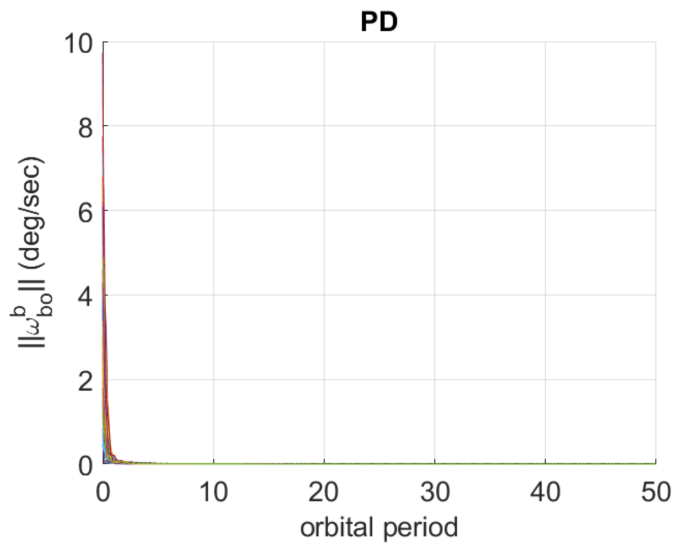
The 40 time behaviors of $\phi$ and of $\parallel {\mathit{\omega }}_{bo}^b\parallel$ obtained in the considered simplified scenario are represented in Figure 2 and Figure 3.

The time histories show that PD control is able to stabilize the nominal attitude even for large initial tumbling conditions.

Regarding the FFDL-MFAC algorithm described by Equations (2)–(8), to the best of the authors’ knowledge, a stability analysis is still an open problem ([26] Section 5.4.1.3). Thus, the numerical values of the MFAC parameters are selected by trial-and-error and are reported in

Table 5. MFAC parameters.

Parameter	Value	Unit
$T_s$	0.1	sec
$L_y$	1
$L_u$	0
$\lambda$	1.2
${\rho }_1={\rho }_2$	0.2
$\mu =\eta$	1
${\mathbf{C}}_1$	${10}^5·$ diag(5 150 0.1)
${\mathbf{C}}_2$	${10}^9·$ diag(0.8 1 0.8)
${\widehat{\mathsf{\Phi }}}_{L_y,L_u}\left(0\right)$	${\mathbf{I}}_{3\times 3}$

.

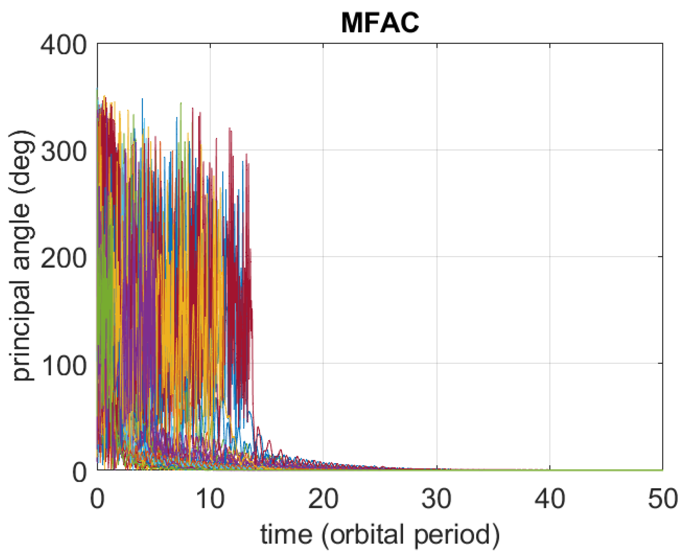
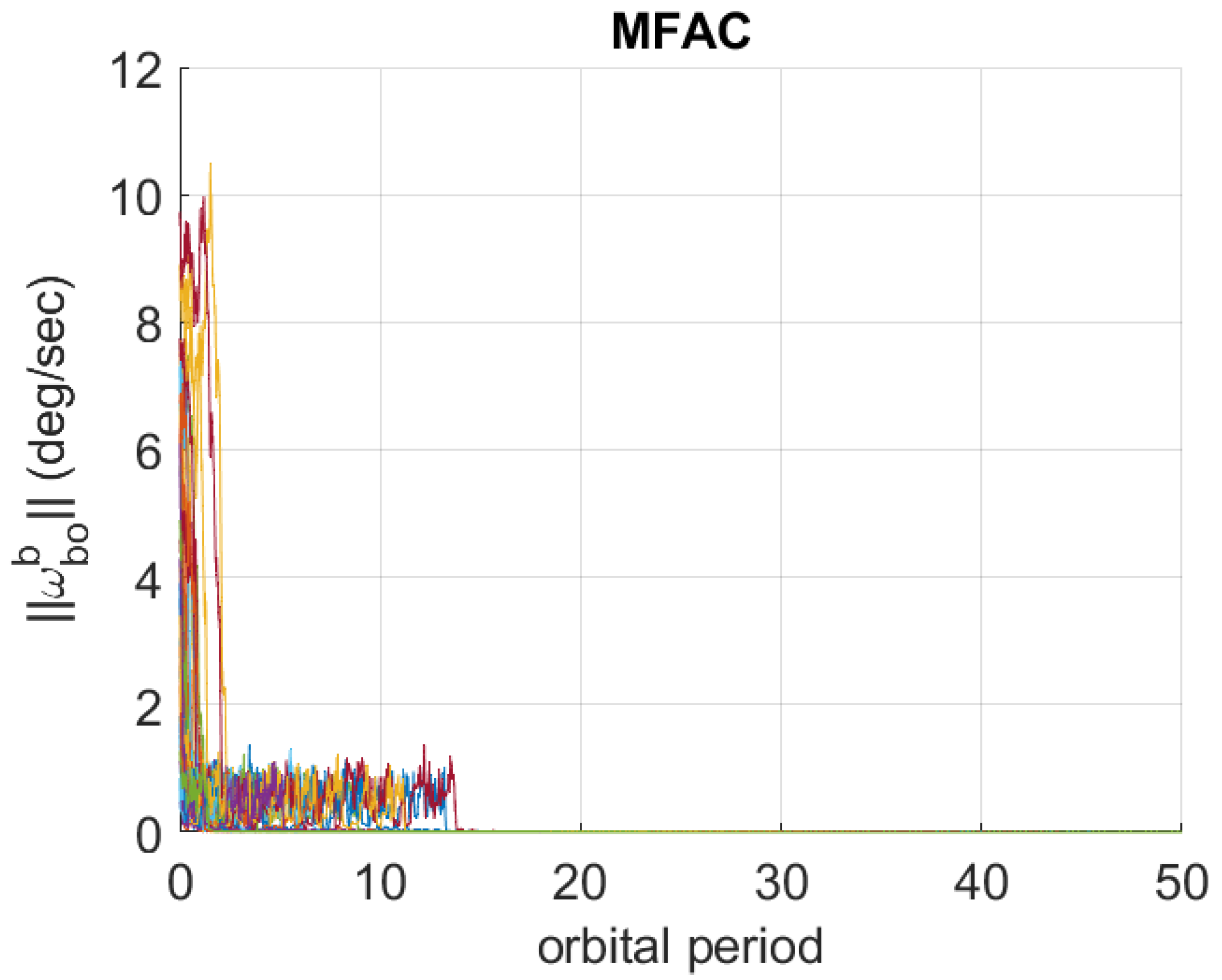
The MFAC algorithm is validated numerically first considering the same simplified scenario as for the validation of PD control. As a result, a new Monte Carlo campaign of 40 simulation runs with the same initial conditions as in the previous campaign is executed with MFAC replacing PD. The corresponding 40 time behaviors of the principal angle of rotation and of $\parallel {\mathit{\omega }}_{bo}^b\parallel$ are represented in Figure 4 and Figure 5.

The time histories show that MFAC is also able to stabilize the nominal attitude even for large initial tumbling conditions.

The effectiveness of the MFAC algorithm is evaluated more thoroughly by running more realistic numerical simulations. In those simulations, the disturbance torques in Equations (14), (15) and (17) are included. The geomagnetic field data are generated by using the International Geomagnetic Reference Field (IGRF) [42,44], which is more accurate than the axial dipole model in Equation (20). Navigation errors are introduced by adding Gaussian noise to ${\mathbf{q}}_v$ and ${\mathit{\omega }}_{bo}^b$ with standard deviations equal to ${10}^{-4}$ and ${10}^{-5}$ deg/s, respectively. The magnetometer’s measurement noise is modeled as a Gaussian noise with standard deviation equal to $3·{10}^{-9}$ T. In each simulation, the initial quaternion $\mathbf{q}\left(0\right)$, the initial angular velocity ${\mathit{\omega }}_{bo}^b\left(0\right)$, and the initial value of the spacecraft argument of latitude $u_0$ are all randomly selected as in the previous Monte Carlo campaign. In addition, the Earth’s angle of rotation at $t=0$ denoted by ${\varphi }_0$ (the Earth’s angle of rotation is the angle between the vernal equinox axis and the axis on the equatorial plane from the Earth’s center to the Earth’s prime meridian) is randomly selected with a uniform distribution over $\left[02\pi \right]$. Thus, a new Monte Carlo campaign with 40 simulation runs has been executed, and in such a scenario, the performances of the proposed MFAC method are compared with those of the following PD control:

$${\mathbf{m}}_{coils}={\mathbf{b}}^b\times (-k_p{\mathbf{q}}_v-k_d{\mathit{\omega }}_{bo}^b)-{\widehat{\mathbf{m}}}_{rm}^b$$

(22)

where the values of $k_p$ and $k_d$ are kept as those indicated in Table 3, and ${\widehat{\mathbf{m}}}_{rm}^b$ denotes an estimate of the residual dipole moment ${\mathbf{m}}_{rm}^b$, which is determined through a Kalman filter [11]. The term $-{\widehat{\mathbf{m}}}_{rm}^b$ partially compensates for the residual magnetic torque in Equation (14), leading to an improvement in three-axis pointing accuracy.

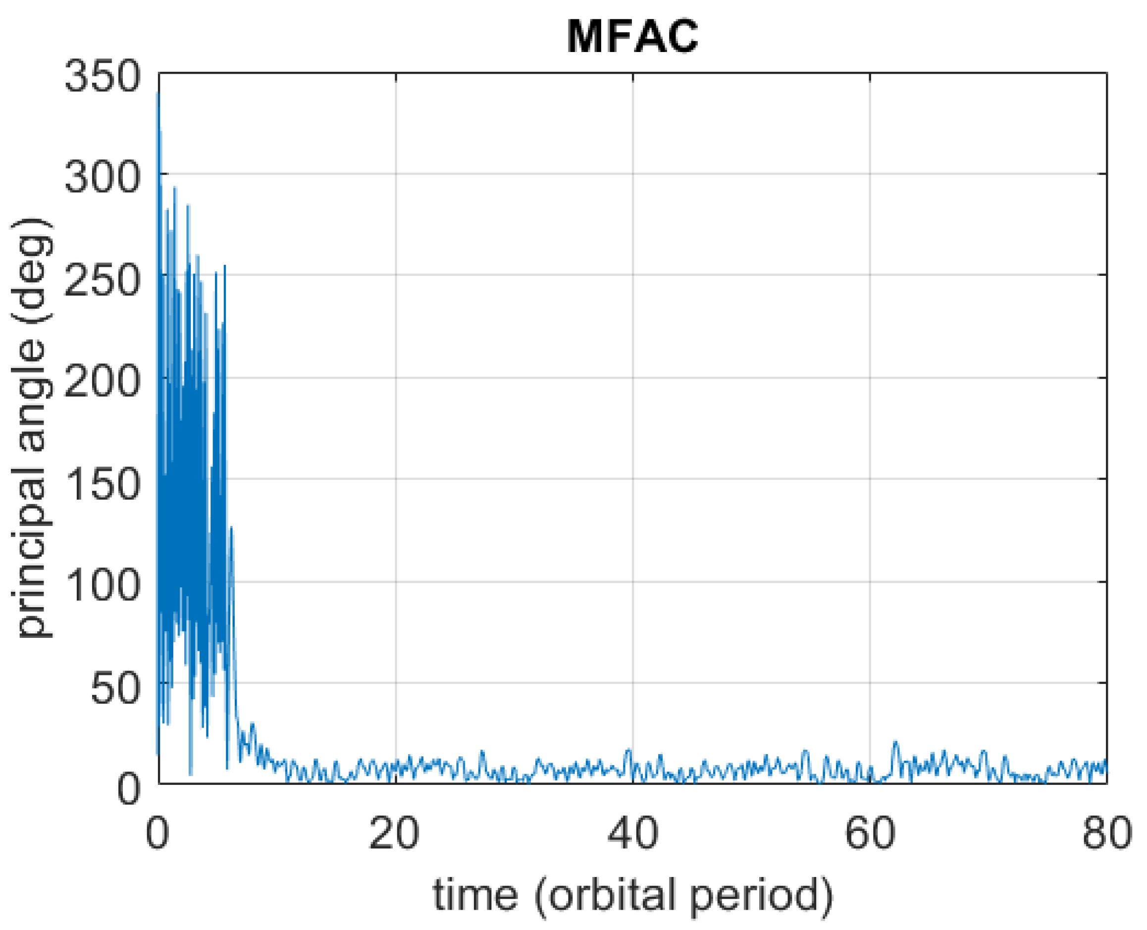
Figure 6 displays a sample time behavior out of the 40 for the principal angle of rotation obtained using MFAC.

The initial conditions employed to generate the plot are indicated in

Table 6. Initial conditions employed to generate the plots in Figure 6 through Figure 11.

Parameter	Unit	Initial Condition
$\mathbf{q}\left(0\right)$		$\left[\begin{array}{c}0.0994\\ -0.0602\\ -0.0513\\ 0.9919\end{array}\right]$
${\mathit{\omega }}_{bo}^b\left(0\right)$	deg/s	$\left[\begin{array}{c}-0.0062\\ -0.0019\\ -0.0482\end{array}\right]$
$u_0$	deg	293.3
${\varphi }_0$	deg	326.1

.

Figure 7 displays the corresponding time behavior of the principal angle of rotation obtained by using PD control in Equation (22).

In these figures as well as in those that follow, the remaining 39 time behaviors are not showcased to obtain representations that can be read more easily. It occurs that in all 40 simulation runs, both MFAC and PD are able to effectively stabilize the nominal attitude.

To compare the performances of MFAC and PD control in terms of accuracy in three-axis alignment, the maximum value of the principal angle of rotation in the steady state is determined.

Table 7. Statistics on maximum principal angle of rotation in steady state.

Maximum Principal Angle in Steady State	Unit	PD	MFAC	Variation
Mean value	deg	28.75	17.61	$-39\%$
Standard deviation	deg	2.39	1.16	$-51\%$

reports the mean values and standard deviations of those maximum values.

The statistics show that MFAC leads to significant reductions in both the mean values and the standard deviations of the principal angle in the steady state. Thus, in this numerical study, MFAC is able to achieve better three-axis pointing accuracy than PD control, which implies that MFAC is able to better compensate for the disturbance torques.

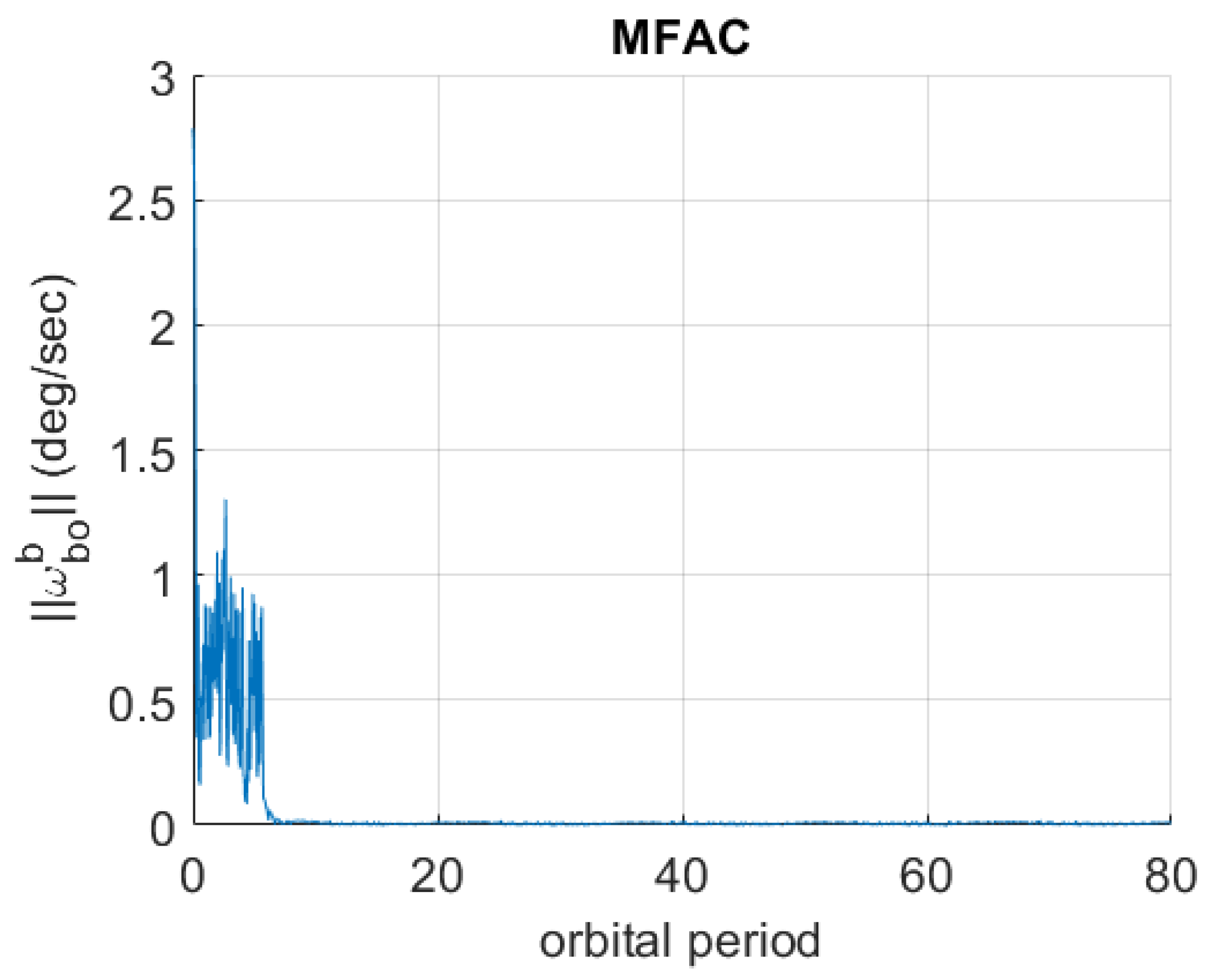
Figure 8 showcases a sample time history out of the 40 $\parallel {\mathit{\omega }}_{bo}^b\parallel$ obtained by using MFAC.

To evaluate the ability of both MFAC and PD control to make ${\mathit{\omega }}_{bo}^b$ converge to zero, for each simulation run, the maximum value of $\parallel {\mathit{\omega }}_{bo}^b\parallel$ is determined once a steady-state condition is reached.

Table 8. Statistics on maximum $\parallel {\mathit{\omega }}_{bo}^b\parallel$ in steady state.

Maximum $\parallel {\mathit{\omega }}_{\mathit{b}\mathit{o}}^{\mathit{b}}\parallel$ in Steady State	Unit	PD	MFAC	Variation
Mean values	deg/sec	1.83·10−2	1.84·10−2	$+0.6\%$
Standard deviations	deg/sec	2.2·10−3	1.6·10−3	$-29\%$

reports the mean values and standard deviations of those maximum values.

The statistics show that in this numerical study, PD and MFAC are able to achieve convergence to zero of $\parallel {\mathit{\omega }}_{bo}^b\parallel$ with comparable accuracy.

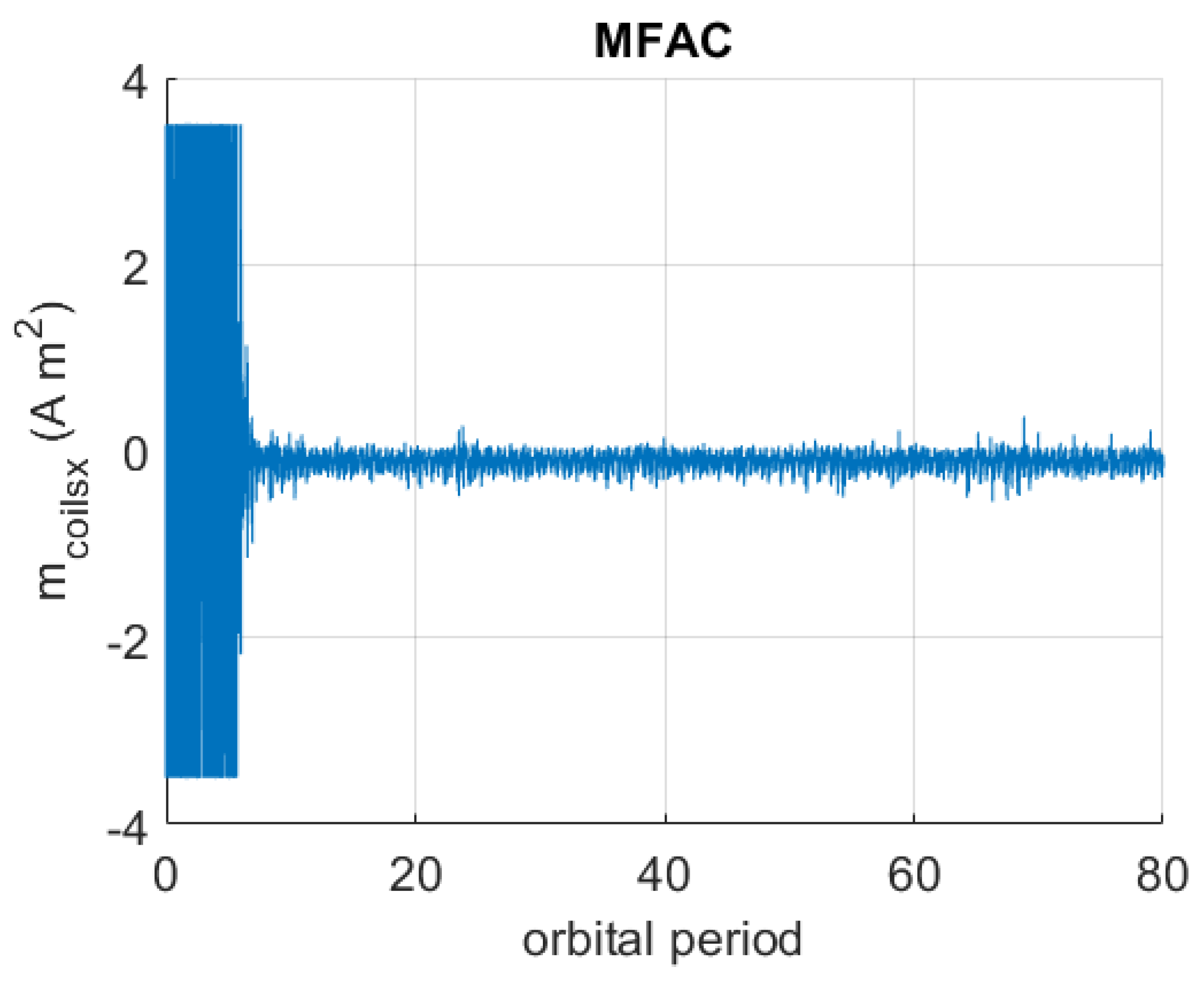
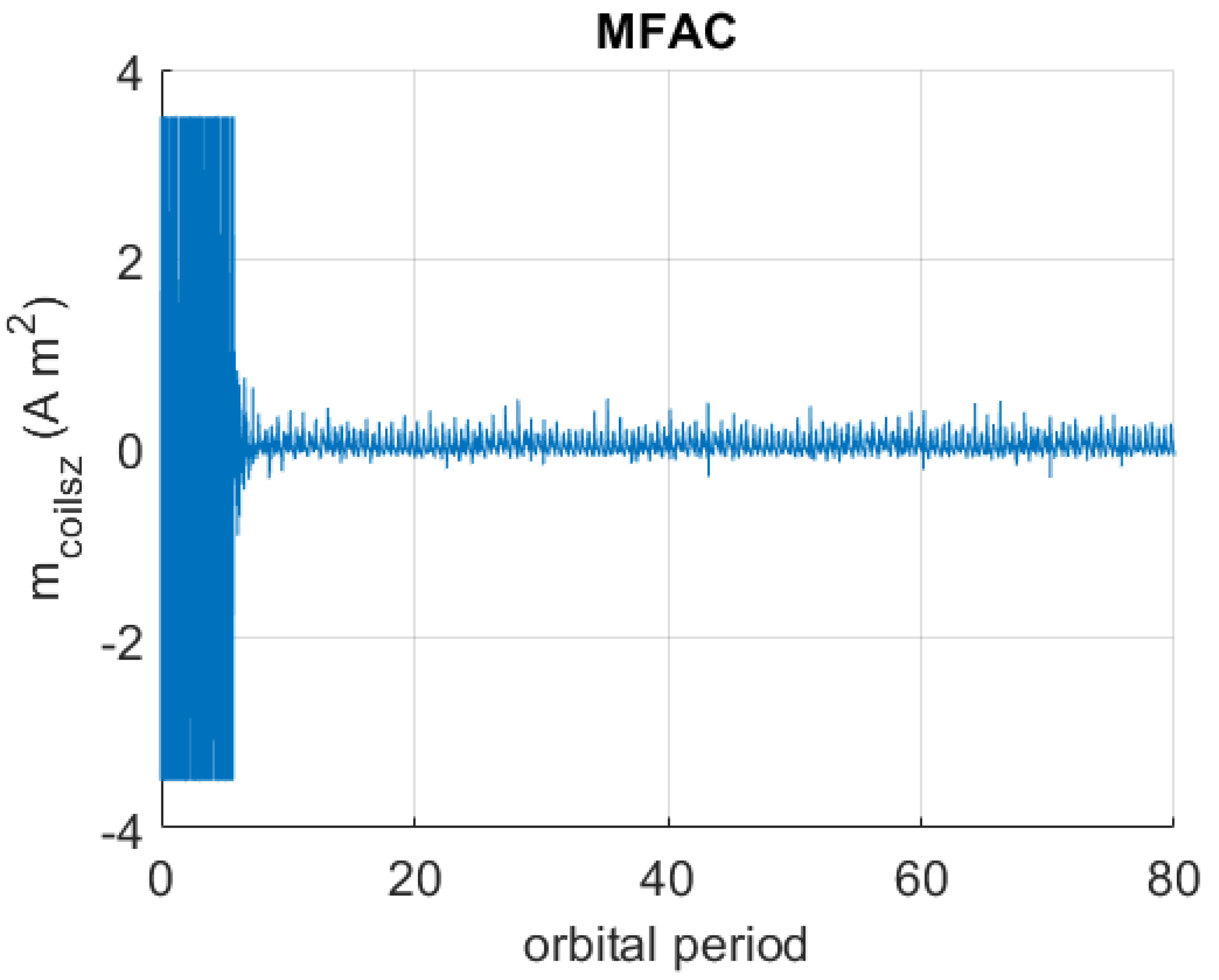
Figure 9, Figure 10 and Figure 11 display a sample time behavior of the control magnetic dipole moment generated by magnetorquers using MFAC, out of the 40 time behaviors.

It is of interest to compare the performances obtained with MFAC and PD control in terms of the energy employed by magnetorquers to stabilize the spacecraft’s attitude. A rough and indirect measure of the latter energy is given by

$${\mathcal{E}}_{coils}={\int }_0^{t_f}{\parallel {\mathbf{m}}_{coils}\left(t\right)\parallel }^{2}dt$$

(23)

where $t_f$ denotes the final simulation time, which is set equal to 80 orbital periods.

Table 9. Statistics on ${\mathcal{E}}_{coils}$.

${\mathcal{E}}_{\mathit{c}\mathit{o}\mathit{i}\mathit{l}\mathit{s}}$	Unit	PD	MFAC	Variation
Mean value	A2 m4 sec	$4.75\times {10}^5$	$7.32\times {10}^5$	$+54\%$
Standard deviation	A2 m4 sec	$7.33\times {10}^5$	$5.78\times {10}^5$	$-21\%$

reports the mean values and standard deviations of ${\mathcal{E}}_{coils}$.

The statistics show that employing MFAC leads to a significant increase in the mean value of ${\mathcal{E}}_{coils}$. Thus, in this numerical study, MFAC consumes significantly more energy to obtain substantially higher pointing accuracy.

5. Discussion

This work shows the effectiveness of employing FFDL-MFAC for three-axis stabilization of the attitude of a spacecraft pointing to the Earth using only magnetic torque actuators. Numerical simulations for a case study show that the proposed control algorithm is able to achieve a good pointing accuracy starting from a random tumbling condition. A comparative analysis with a model-based PD control reveals the superiority of MFAC in terms of pointing accuracy at the cost of a higher energy consumption. These findings confirm that MFAC is an effective algorithm in spacecraft attitude control.