Article

Trajectory Segmentation and Clustering in Terminal Airspace Using Transformer–VAE and Density-Aware Optimization

College of Civil Aviation, Nanjing University of Aeronautics and Astronautics, Nanjing 211106, China
*
Author to whom correspondence should be addressed.
Aerospace 2025, 12(11), 969; https://doi.org/10.3390/aerospace12110969
Submission received: 5 September 2025 / Revised: 22 October 2025 / Accepted: 24 October 2025 / Published: 30 October 2025
(This article belongs to the Section Air Traffic and Transportation)

Abstract

Clustering of aircraft trajectories in terminal airspace is essential for procedure evaluation, flow monitoring, and anomaly detection, yet it is challenged by dense traffic, irregular sampling, and diverse maneuvering behaviors. This study proposes a unified framework that integrates dynamics-aware segmentation, Transformer–Variational Autoencoder (Transformer–VAE)-based representation learning, and density-aware clustering with joint optimization. A dynamic-feature Minimum Description Length (DFE-MDL) algorithm is introduced to preserve maneuver boundaries and reduce reconstruction errors, while the Transformer–VAE encoder captures nonlinear spatiotemporal dependencies and generates compact latent embeddings. Clusters are initialized using Hierarchical Density-Based Spatial Clustering of Applications with Noise (HDBSCAN) and further refined through Kullback–Leibler (KL) divergence minimization to improve consistency and separability. Experiments on large-scale ADS-B data from Guangzhou Baiyun International Airport, comprising over 27,000 trajectories, demonstrate that the framework outperforms conventional geometric and deep learning baselines. Results show higher reconstruction fidelity, clearer cluster separation, and reduced computation time, enabling interpretable flow structures that reflect operational practices. Overall, the framework provides a data-driven and scalable approach for terminal-area trajectory analysis, offering practical value for STAR/SID compliance monitoring, anomaly detection, and airspace management.

1. Introduction

The continuous growth of global air traffic has intensified concerns regarding the safe and efficient operation of terminal airspace. As the critical interface between en route and runway phases, terminal areas are distinguished by compressed vertical separation, intricate route structures, and frequent sequencing constraints. Although these phases represent only a small fraction of total flight time, they contribute disproportionately to conflicts, delays, and safety incidents. According to the ICAO Annual Safety Report [1], more than 60% of safety-related events occur during approach and departure. Long-term forecasts, including the Eurocontrol Challenges of Growth report [2], the SESAR European ATM Master Plan [3], and the ICAO Global Air Navigation Plan [4], consistently identify terminal-area safety and efficiency as persistent bottlenecks for the sustainable development of global air transport.
To address these risks, data-driven methods for analyzing aircraft trajectory patterns have attracted increasing attention in both research and practice. Among these, clustering has emerged as a promising technique for traffic flow monitoring, operational procedure evaluation, and anomaly detection [5,6]. By extracting representative structures from large-scale trajectory datasets, clustering provides valuable insights that can support airspace redesign, inform revisions of standard instrument procedures, and enhance conflict detection in high-density environments. Nonetheless, the direct application of clustering to terminal-area operations remains highly challenging. Unlike en route trajectories, which tend to be smoother and more predictable, terminal-area trajectories are strongly shaped by continuous air traffic control (ATC) interventions, dynamic environmental conditions, and heterogeneous flight intents. These influences result in data that often exhibit irregular sampling rates, abrupt heading or speed changes, and diverse maneuvering behaviors. Such characteristics complicate the discovery of underlying structural patterns and reveal the limitations of conventional clustering methods, which typically rely on assumptions of smoothness or homogeneity.
In response to these challenges, recent studies have incorporated advanced data-driven techniques—such as nonlinear dimensionality reduction, probabilistic modeling, and density-based clustering—into trajectory analysis. While these approaches have improved robustness and interpretability, they often rely on handcrafted features, assume fixed clustering structures, or struggle to scale under real-world traffic conditions. As a result, there remains a clear need for a more integrated framework capable of adaptively segmenting trajectories, capturing nonlinear spatiotemporal dependencies, and producing operationally coherent clusters under complex and dynamic environments.
To this end, this study proposes a unified trajectory clustering framework that integrates segmentation, representation learning, and clustering within a single pipeline.
First, a dynamic-feature Minimum Description Length (DFE-MDL) algorithm is applied to identify motion-consistent breakpoints that preserve critical structural and dynamic information. By incorporating speed variation and heading-rate change as dynamic cues, the segmentation process becomes more robust to noise and better aligned with genuine motion transitions in terminal operations. Second, a Transformer–Variational Autoencoder (Transformer–VAE) model is designed to encode nonlinear spatiotemporal dependencies, enabling the construction of compact and discriminative latent representations. Here, the Transformer–VAE refers to a deep representation framework that integrates the sequential modeling capability of the Transformer with the latent-space learning of a Variational Autoencoder (VAE).Unlike previous studies that treat representation learning and clustering as separate processes, the proposed framework jointly optimizes both through a Kullback–Leibler (KL) divergence-based density-aware objective, thereby enhancing consistency between latent embeddings and cluster assignments. The clustering module is initialized with Hierarchical Density-Based Spatial Clustering of Applications with Noise (HDBSCAN)—a robust density-based algorithm capable of identifying clusters of varying densities without requiring a predefined number of clusters—and is subsequently refined through the same KL-divergence-based joint optimization to improve cluster cohesion and interpretability. This integrated design enables the framework to capture complex spatiotemporal structures more effectively than conventional autoencoder- or Principal Component Analysis (PCA)-based clustering approaches.
Extensive experiments using Automatic Dependent Surveillance–Broadcast (ADS-B) data from Guangzhou Baiyun International Airport demonstrate that the proposed framework consistently outperforms conventional baselines in terms of clustering quality, robustness, and operational interpretability.

1.1. Literature Review

Research on aircraft trajectory clustering has progressed from conventional similarity-based methods to advanced deep learning approaches and domain-specific frameworks for terminal operations. Early studies employed geometric or distance measures such as Hausdorff, Fréchet, and dynamic time warping, combined with K-Means, DBSCAN, or Gaussian Mixture Models [7,8,9,10,11]. These methods are computationally efficient and interpretable, but they are highly sensitive to noise and irregular sampling, and their reliance on fixed-length representations limits the ability to capture dynamic flight behaviors. Their applicability in complex terminal environments is further constrained by parameter sensitivity and the assumption of a predefined number of clusters [9,10].
With the advent of deep learning, trajectory representation learning has advanced from shallow dimensionality reduction methods, including PCA and simple autoencoders [12], to more powerful architectures such as Variational Autoencoders (VAEs) and Transformers [13,14,15]. Neural embeddings have proven effective in capturing nonlinear spatiotemporal dependencies [5,6,15], and extensions such as temporal convolutional autoencoders [16] or multi-scale attention models [17] have been applied to trajectory prediction and clustering. Nevertheless, most of these methods learn representations independently of clustering, leaving the latent space misaligned with clustering objectives. Moreover, key aviation dynamics—such as heading rate, vertical speed, and coordinated turns—are often underrepresented, limiting the operational interpretability of the results [16,17].
Parallel research has examined segmentation and similarity measures as essential tools for uncovering interpretable structures. Threshold-based methods using heading or speed changes [7,8] are simple but noise-sensitive, while MDL-based segmentation reduces approximation errors at the cost of heuristic assumptions [18,19]. Broader surveys have compared spatial–temporal similarity measures [20,21,22,23], and adaptive methods such as reinforcement-based online segmentation [24] have been introduced. However, segmentation and similarity learning are typically studied in isolation from representation learning and clustering, leaving integration gaps unaddressed.
Several works have focused specifically on terminal airspace. Examples include deep autoencoders combined with Gaussian Mixture Models [25], probabilistic trajectory modeling approaches tailored to terminal airspace operations [26], Fréchet-based multi-level refinements [27], and unified spatial–temporal similarity metrics [22]. Large-scale evaluations of similarity functions [23], unsupervised flow identification [28], visualization frameworks [29] further highlight ongoing efforts. While these studies underscore the need for tailored solutions, segmentation, representation, and clustering are generally addressed separately, which limits generalizability and scalability in operational environments.
In summary, although previous studies have provided valuable insights and contributed important methodological advances, they generally fall short of integrating segmentation, representation learning, and clustering into a cohesive framework. At the same time, the underutilization of aviation-specific dynamic features and the limited availability of large-scale validations in real terminal operations constrain both interpretability and practical applicability. These gaps motivate the unified framework proposed in this study, which combines dynamic-feature segmentation, Transformer–VAE-based embedding, and density-aware clustering with joint optimization to address the challenges of complex terminal-area operations.

1.2. Our Contributions

This paper proposes a unified framework for trajectory clustering in terminal airspace and makes several contributions to the existing literature:
(1)
We develop a dynamic-featured segmentation algorithm (DFE-MDL) that incorporates speed variation and heading rate into the description length criterion, thereby improving robustness under irregular sampling and maneuvering noise while preserving critical trajectory structures.
(2)
We design a Transformer–VAE model for representation learning and couple the encoder with clustering assignments through a joint optimization procedure, enabling the generation of compact and separable latent embeddings that enhance clustering consistency.
(3)
We validate the proposed framework using large-scale ADS-B data collected from a busy terminal area, and the results demonstrate notable improvements in clustering quality, trajectory discrimination, and computational efficiency, confirming its operational relevance in complex terminal environments.

1.3. Organization of This Paper

The remainder of this paper is organized as follows. Section 2 presents the proposed methodology, covering trajectory preprocessing, dynamic segmentation, latent representation learning, cluster initialization, and joint optimization. Section 3 reports the experimental results, including evaluations of segmentation, representation learning, and clustering performance, as well as a large-scale efficiency analysis. Section 4 concludes the study and discusses potential directions for future research.

2. Methodology

2.1. Overview of the Proposed Method

To address the challenges of clustering flight trajectories in terminal airspace, a multi-stage unsupervised framework is developed. The framework integrates preprocessing, dynamic segmentation, latent representation learning, density-based initialization, and joint optimization. Its objective is to derive structurally coherent clusters directly from raw Automatic Dependent Surveillance–Broadcast (ADS-B) data without relying on predefined routes or intent labels.
As shown in Figure 1, the framework consists of five main components:
Data Processing: Raw ADS-B trajectories are first cleaned to remove missing or duplicated points and then converted from geodetic coordinates to a local East–North–Up (ENU) reference frame. In addition to positional and velocity information, dynamic indicators—such as acceleration, heading change rate, and climb/descent rate—are derived to enrich trajectory features. This step establishes a standardized representation of the data, ensuring consistency for subsequent segmentation.
Trajectory segmentation: A Minimum Description Length-based segmentation algorithm is applied, incorporating both geometric and dynamic attributes. This enables the detection of motion-consistent breakpoints under irregular sampling conditions while reducing the impact of noise and maneuvering variability. The resulting sub-trajectories provide structured inputs that capture local dynamics, which are essential for effective representation learning.
Latent representation via Transformer–VAE: Each segmented sub-trajectory is encoded using a Transformer-based variational autoencoder. The model captures long-range temporal dependencies and spatiotemporal continuity, mapping trajectories into a compact latent space suitable for clustering. In this way, complex raw trajectories are transformed into low-dimensional embeddings that retain the structural information revealed by segmentation.
Cluster initialization with HDBSCAN: Density-based clustering is performed in the latent space using HDBSCAN, which automatically determines the number of clusters and identifies noise trajectories commonly present in operational data. This stage leverages the separable latent representations to produce an initial partition, serving as the foundation for refinement.
Joint optimization: Finally, clustering assignments and encoder parameters are refined jointly. By minimizing the Kullback–Leibler divergence between soft assignments and an adaptive target distribution, intra-cluster compactness and inter-cluster separability are enhanced. This step links representation learning and clustering objectives, closing the loop and producing stable, interpretable trajectory clusters.
The proposed framework is fully unsupervised and applicable to both arrival and departure flows in terminal areas. By representing diverse operational structures in a unified manner, it provides a basis for subsequent tasks such as flow monitoring, anomaly detection, and procedure evaluation.

2.2. Data Preprocessing

Raw ADS-B data provide time-ordered flight states, including position, altitude, speed, and heading. Quality control is performed by removing trajectories with more than 30% missing values, eliminating outliers using a 3σ filter on velocity and heading, and discarding redundant samples based on a minimum Euclidean distance threshold. All features are subsequently normalized using Z-score standardization to ensure comparability across dimensions.
For spatial analysis, geographic coordinates must be expressed in a locally consistent Cartesian system. To this end, raw WGS-84 geodetic coordinates are converted into a local East–North–Up (ENU) frame centered at the airport. This two-step conversion ensures that Euclidean distances and directional changes can be directly computed, which is essential for segmentation and clustering.
  • WGS−84 to Earth-Centered Earth-Fixed (ECEF):
The first step maps latitude, longitude, and altitude onto the Earth-centered Cartesian system. This transformation removes the curvature dependency of geodetic coordinates, providing a globally uniform reference frame.
N = α 1 e 2 s i n φ X = ( N + h ) c o s φ c o s λ Y = ( N + h ) cos φ sin λ Z = ( ( 1 e 2 ) N + h ) s i n φ
where φ denotes latitude (°),  λ denotes longitude (°),  h is the altitude relative to the WGS-84 ellipsoid (m),  α is the semi-major axis of the WGS-84 ellipsoid (m),  e is the eccentricity of the WGS-84 ellipsoid,  N (m) is the radius of curvature in the prime vertical.
2.
Convert ECEF to ENU using a reference point:
The second step converts the ECEF representation into a local ENU system centered at the airport. This local frame aligns axes with east, north, and up directions, simplifying trajectory comparison and allowing spatial relationships to be interpreted relative to the terminal area.
X E N U Y E N U Z E N U = sin λ 0 cos λ 0 0 sin φ 0 cos λ 0 sin φ 0 sin λ 0 cos φ 0 cos φ 0 cos λ 0 cos φ 0 sin λ 0 sin φ 0 X X 0 Y Y 0 Z Z 0
where (X,Y,Z) are the coordinates of a trajectory point in the ECEF frame (m), ( X E N U , Y E N U , Z E N U ) are the transformed coordinates in the local ENU frame (m), with axes aligned to east, north, and up directions, respectively,  φ 0 , λ 0 , h 0 , reference point centered at the airport,  X 0 , Y 0 , Z 0 , ECEF coordinates of the reference point.
  • To enrich the motion description, several dynamic features are derived. Specifically:
  • Speed change rate:
Δ v i = v i v i 1 t i t i 1
where  v i is the ground speed at point  i (m/s),  t i is the timestamp at point  i (s), and  Δ v i denotes the speed change rate (m/s2).
  • Heading angle change rate:
Δ θ i = θ i θ i 1 t i t i 1
where  θ i denotes the heading angle at point  i (°), and  Δ θ i represents the heading change rate (°/s).
  • Linear acceleration:
a i = v i 2 v i 1 2 2 Δ s i
where  Δ s i is the horizontal distance between points i and i 1 (m), and  a i the linear acceleration (m/s2).

2.3. Trajectory Segmentation

To extract meaningful structural segments while preserving dynamic information, each trajectory is processed using a segmentation algorithm grounded in the Minimum Description Length (MDL) principle. The objective is to identify a set of breakpoints that minimizes the total description cost, thereby balancing model complexity and approximation fidelity.
Let the original trajectory be defined as follows:
T = { p 1 , , p T } , p i = x i , y i , z i , v i , Δ v i , χ i , Δ χ i , t i
where each point  p i consists of positional coordinates and dynamic attributes (e.g., speed  v i , speed change rate  Δ v (m/s), heading angle  χ i and heading angle change rate  Δ χ (deg/s),  t i time). Including the variation terms of speed and heading allows the segmentation algorithm to distinguish genuine maneuvering behaviors (e.g., turns or accelerations) from random measurement fluctuations, thereby improving robustness and ensuring that detected breakpoints correspond to physically meaningful motion changes.
The trajectory is partitioned into  k line segments by a set of breakpoints  B = { b 0 = 1 , b 1 , , b k = T } , each  b j 1 , b j defines a segment. The total description length for a given segmentation is expressed as follows:
L t o t a l = L m o d e l + L e r r o r
Assuming a 3D linear model for each segment, the model cost is proportional to the number of segments:
L m o d e l = α k
where  α is a weighting factor reflecting model complexity,  k is number of segments.
The error term captures both spatial deviation and dynamic discrepancy between the original trajectory and its linear approximation:
L e r r o r = i = 1 n λ 1 p i p ^ i + λ 2 f i f ^ i ,
Here,  f i = v i , χ i represents the dynamic state and  p ^ i f ^ i denote their respective linear approximations. Coefficients  λ 1 λ 2 balance the influence of spatial and dynamic reconstruction error.
To improve computational efficiency, candidate breakpoints are restricted to local peaks of a composite dynamic change rate:
Δ t = d v d t 2 + C d χ d t 2 ,
To maintain physical consistency, a dimensional coefficient  C = 1 , m 2 / ( rad 2 , s 2 ) is introduced to the angular-rate term. This ensures that the dynamic change rate  Δ t remains invariant under unit transformations.
The set of candidate breakpoints is then defined as follows:
B cand = t i Δ t i is   a   local   maximum ,
The optimal set of breakpoints  B B cand is determined by minimizing the total cost:
B = arg min B B cand L total ,
This optimization can be solved using greedy search or dynamic programming. After segmentation, each trajectory is uniformly resampled to a fixed length by linear interpolation to ensure compatibility with downstream neural encoders.

2.4. Derivation of Dynamic and Geometric Features

Given  T steps and hidden size  d h , the encoder/decoder each scale as  O ( L T 2 d h ) due to self-attention mechanism, while the VAE heads add  O ( d h d z ) , where  d z denotes the dimension of the latent variable vector  z in the variational bottleneck. In practice  T 128 keeps runtime feasible for large-scale batches.
Figure 2 Architecture of the Transformer–VAE model used for trajectory representation learning. The input sequence  X is processed by four layers of Transformer encoders. The resulting latent vector  z is sampled and fed into a symmetric Transformer decoder to reconstruct the sequence  X . The model is optimized using a combination of reconstruction loss and KL divergence.
The model consists of four stacked Transformer encoder layers and four symmetric decoder layers (indicated by “×4”) used for trajectory representation learning.
The purple blocks represent input and output trajectory sequences, while the green trapezoids denote the encoder and decoder modules.
Different colors are used only to visually distinguish the network components.
To obtain compact trajectory representations that preserve spatiotemporal and dynamic characteristics, we employ a Transformer-based variational autoencoder (Transformer–VAE). The model encodes each segmented trajectory into a fixed-dimensional latent vector, which is then used for downstream clustering.
Let the preprocessed and segmented trajectory be  X T × d , where  T is the resampled sequence length and  d = 6 is the feature dimension including normalized ENU  ( E , N , U ) position in meters, ground speed  v (m/s), heading angle  χ (deg), vertical rate (m/s), speed change rate  Δ v (m/s), and heading change rate  Δ χ (deg/s). All continuous variables are standardized to zero mean and unit variance.
The encoder is a stack of  L Transformer layers with multi-head self-attention and position-wise feed-forward networks (FFNs), each followed by residual connections, layer normalization, and dropout.
Given input  X , the encoder produces hidden states:
H = TransformerEncoder ( X ) T × d h , where  d h is the hidden size and  H t d h denotes the  t -th row of  H .
To obtain a fixed-size code, we apply temporal average pooling:
h avg = 1 T t = 1 T H t d h ,
Remark, other reductions (CLS token, attention pooling, max/mean mix) were tested; average pooling offered the best stability-to-accuracy trade-off in our setting.
Two linear heads project  h avg to the mean and log-variance of a diagonal Gaussian:
μ = W μ h avg + b μ , log σ 2 = W σ h avg + b σ , with  W μ , W σ d z × d h and b μ , b σ d z , where  d z is the latent dimension.
The latent vector is sampled via the reparameterization trick:
σ = exp 1 2 log σ 2 , z = μ + σ ϵ , ϵ ~ N ( 0 , I d z ) , z d z
The decoder mirrors the encoder architecture. The latent code  z is linearly projected to  d h , repeated to length  T ( T = T in our experiments), and combined with positional encodings before passing through  L Transformer decoder layers to produce  X T × F . Padding masks are applied when variable-length inputs are used.
The model is trained to minimize a reconstruction term plus a KL regularizer:
L rec = 1 n i = 1 n X ( i ) X ( i ) 2 2 ,
L KL = 1 2 j = 1 d z ( 1 + log σ j 2 μ j 2 σ j 2 ) ,
L VAE = L rec + β KL L KL ,
Here n is the batch size  μ j σ j are the  j elements of  σ ; and  β KL [ 0 , 1 ] controls the strength of the regularize. We use KL annealing (linear warm-up from 0 to 1) to avoid posterior collapse and encourage informative latent factors.
If feature channels require balancing, a weighted reconstruction loss is used:
L rec = 1 n i t , f w f ( X t , f ( i ) X ^ t , f ( i ) ) 2   with   f w f = 1 ,
where  w f is the weight for channel  i .

2.5. Cluster Initialization and Joint Optimization

To assign latent trajectory embeddings into coherent groups, we adopt a two-stage clustering procedure. First, initial clusters are identified using a density-based algorithm. Then, the encoder and cluster assignments are refined iteratively through soft assignment learning and KL divergence minimization.
  • Initial Cluster Assignment via HDBSCAN
After extracting the latent vectors  z i d z , initial clusters are obtained using the Hierarchical Density-Based Spatial Clustering of Applications with Noise (HDBSCAN). Unlike K-Means, HDBSCAN does not require the number of clusters to be predefined and can identify noise points based on local density.
Given a set of latent embeddings  z = z 1 , z 2 , z N , HDBSCAN produces A cluster label  y i { 1 , , K } { 1 } , where −1 denotes noise; A set of cluster centers { μ j } j = 1 K , computed as the mean of latent vectors in each cluster.
Trajectories labeled as noise are excluded from subsequent optimization.
2.
Soft Assignment and Target Distribution
To enable differentiable learning of cluster structure, soft assignment probabilities between each latent vector  z i and cluster center  μ j are computed using the student’s t-distribution kernel:
q i j = 1 + z i     μ j 2 γ γ   +   1 2 j 1 + z i μ j 2 γ γ   +   1 2 ,
where  γ is the degree of freedom, typically set to 1.
To emphasize high-confidence assignments, a target distribution  p i j is defined as follows:
p i j = q i j 2 / i q i j j q i j 2 / i q i j ,
which increases the influence of confident samples while reducing the impact of ambiguous ones.
3.
Optimization Objective and Training Procedure
The clustering objective is defined as the Kullback–Leibler divergence between the target and soft assignment distributions:
L c l u s t e r = i j p i j log p i j q i j ,
The final training loss combines the VAE loss (Section 3.3) with the clustering loss:
L t o t a l = L r e c + β K L L K L + λ c l u s t e r L c l u s t e r ,
where  λ c l u s t e r and  β K L are coefficients balancing reconstruction fidelity, latent regularization, and clustering consistency.
The training process proceeds as follows:
  • Encode all trajectories using the Transformer–VAE to obtain  z i ;
  • Apply HDBSCAN to obtain initial cluster centers  μ j ;
  • Compute soft assignments  q i j and target distribution  p i j ;
  • Update encoder parameters and cluster centers by minimizing  L t o t a l ;
  • Repeat steps 3–4 until convergence criteria are met, such as stabilization of cluster assignments or reduction in KL divergence.
This joint optimization process simultaneously refines the latent representations and the cluster structure, thereby enabling the model to more effectively capture diverse operational patterns in terminal-area trajectory data.

3. Experimental Results

3.1. Dataset

Experiments are conducted on ADS-B trajectory data collected in November 2018 from the terminal area of Guangzhou Baiyun International Airport. The dataset covers both arrival and departure operations within a 50 km radius and altitudes below 6 km. Each record contains position, altitude, ground speed, heading, timestamp, and associated flight identifiers.
After applying the preprocessing pipeline described in Section 2, trajectories with holding patterns, large vectoring deviations, or incomplete records are excluded. A total of 11,563 arrival trajectories and 16,196 departure trajectories are retained. All trajectories are scaled to the range [0,1] using min–max normalization and represented as fixed-length tensors, which serve as standardized inputs to the Transformer–VAE and subsequent clustering modules.
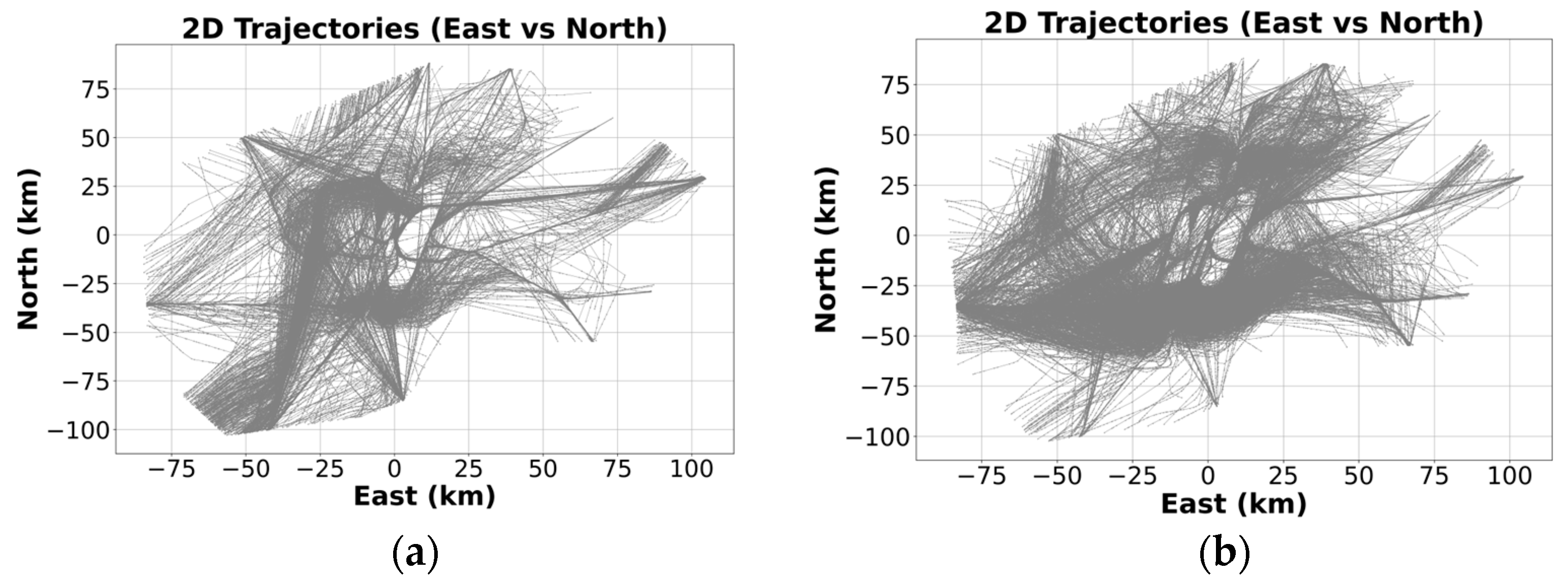
The spatial coverage of the processed trajectories is illustrated in Figure 3a,b, where flows are shown in the ENU reference frame and normalized for downstream analysis.

3.2. Experimental Setup

All experiments were implemented in Python3.10 using PyTorch 2.0. The training was conducted on a workstation equipped with an AMD Ryzen 9 7950X CPU, an NVIDIA RTX 4090 GPU with 24 GB memory, and 64 GB RAM.
Unless otherwise stated, the encoder/decoder stack uses  L = 4 layers, hidden size  d h = 256 , attention heads  = 8 , FFN size  = 1024 d z = 16 , dropout  = 0.1 . The model is trained for 100 epochs using Adam with initial learning rate  10 3 , cosine decay scheduling, batch size 64, and gradient clipping at 1.0. Angular features are unwrapped before differencing to avoid discontinuities at the 360° boundary, and time masks are applied to handle variable-length sequences. All trajectories are preprocessed and normalized as described in Section 2, ensuring that the inputs are consistent across segmentation, representation learning, and clustering modules.

3.3. Evaluation Metrics and Visualization

To assess the effectiveness of the proposed clustering framework, we employ both quantitative metrics and qualitative visualization techniques. These tools evaluate training dynamics, validate the learned latent representation, and compare clustering outcomes against baseline methods.
  • Clustering Evaluation Metrics
The clustering performance is evaluated using four widely adopted indices:
Silhouette Coefficient (SC): Measures the compactness and separation of clusters. Higher SC values indicate better-defined clusters.
S C = 1 N i = 1 N b i a i max ( a i , b i ) ,
where  a i is the average distance from sample x to other points in the same cluster, and  b i is the minimum average distance from x to points in other clusters.
Calinski–Harabasz Index (CH): Computes the ratio of between-cluster dispersion to within-cluster dispersion. A higher score suggests better clustering structure.
CH = Tr ( B k ) Tr ( W k ) N k k 1 ,
where  Tr B k is the trace of the between-group dispersion matrix,  Tr W k is the trace of the within-group dispersion matrix,  N is the number of total samples,  k is the number of clusters.
Davies–Bouldin Index (DB): Represents the average similarity between each cluster and its most similar one. Lower DB values imply better clustering.
DB = 1 k i = 1 k max j i σ i + σ j μ i μ j ,
where  σ i is the average distance from each point in cluster  i to its centroid,    μ i   is the centroid of cluster  i .
Sum of Squared Errors (SSE): Captures the total intra-cluster variance. Lower SSE values indicate tighter clusters.
SSE = j = 1 K x i C j x i μ j 2 ,
These metrics are computed both before and after joint optimization to assess improvements in clustering consistency. Specifically, SSE evaluates intra-cluster compactness (lower values indicate better performance), SC measures cohesion and separation (higher values are preferred), CH captures the ratio of inter- to intra-cluster dispersion (higher values are better), and DB penalizes high intra-cluster variance and low separability (lower values are better). For fair comparison, baseline models are trained using the default settings of scikit-learn unless otherwise specified.
2.
Latent Space Visualization
To provide an intuitive understanding of the learned representations, t-distributed Stochastic Neighbor Embedding (t-SNE) is employed to project the high-dimensional latent vectors into a two-dimensional space. Visual comparisons before and after clustering refinement illustrate the effect of joint optimization on cluster separability.
3.
Optimization Convergence Monitoring
During training, the Kullback–Leibler divergence between the soft assignment distribution and the target distribution is continuously monitored. The evolution of the KL loss reflects the stability of the joint optimization process and the degree of alignment between latent embeddings and cluster structures.

3.4. Verification of the Segmentation Algorithm

The accuracy of the proposed DFE-MDL segmentation method was evaluated against three widely used trajectory simplification algorithms: Uniform Sampling, Douglas–Peucker, and Visvalingam–Whyatt. These methods are commonly applied in aviation and geospatial analysis and thus serve as appropriate benchmarks for assessing reconstruction performance.
For quantitative evaluation, two metrics were employed: Root Mean Square Error (RMSE) and Average Percentage Deviation (APD). RMSE measures the absolute deviation between reconstructed and original trajectories, with higher sensitivity to large errors. APD captures relative deviation normalized by trajectory length, enabling fair comparison across flights of varying scales.
Table 1 summarizes the results. The proposed DFE-MDL achieved the lowest RMSE (0.0294) and APD (0.0187), demonstrating superior reconstruction fidelity, particularly in preserving turning maneuvers, curved segments, and localized structural variations that are often lost in geometry-driven simplification. By contrast, Uniform Sampling produced the highest errors due to its fixed interval selection, while Douglas–Peucker and Visvalingam–Whyatt, though adaptive to curvature or area, exhibited greater deviations in complex segments. By jointly encoding dynamic features and geometric properties within a description length framework, DFE-MDL achieves a balanced trade-off between model complexity and reconstruction accuracy, adapting effectively to diverse trajectory structures. These findings confirm that DFE-MDL provides a reliable and consistent representation suitable for downstream applications such as clustering, anomaly detection, and flow monitoring.
To further assess the performance of different segmentation methods, a qualitative comparison of trajectory reconstructions is presented in Figure 4, where all methods retain 25 representative points (approximately 10% of the original samples) to ensure fair comparison. The results show that the DFE-MDL reconstruction aligns with the original trajectories more accurately, particularly in high-curvature regions, turning maneuvers, and areas with localized variations. In contrast, conventional approaches tend to oversmooth these features, leading to geometric distortion and under-representation of trajectory complexity. These visual differences clearly illustrate that DFE-MDL better preserves local dynamic patterns while maintaining global trajectory consistency.
Uniform Sampling produces coarse approximations due to its non-adaptive point selection strategy. Douglas–Peucker and Visvalingam–Whyatt, although adaptive in nature, under-segment high-curvature regions and oversimplify abrupt directional changes. By contrast, DFE-MDL effectively preserves localized structural details while maintaining global trajectory consistency. These findings further highlight its suitability for applications that demand high-fidelity reconstruction, such as airspace monitoring and trajectory pattern analysis.
Building on the basic segmentation results, trajectory fidelity is further enhanced through a neighborhood expansion strategy applied around the detected breakpoints. This approach increases sampling density in regions of rapid maneuvering, such as sharp turns or abrupt directional changes, while preserving the overall trajectory shape and ensuring global consistency.
Figure 5 illustrates the effect: the left panel shows uniform resampling with 128 points, which produces sparse representations in curved regions; the middle panel shows segmentation with 27 DFE-MDL points, which captures major transitions but lacks local continuity; and the right panel shows neighborhood expansion around key points, providing denser coverage in dynamic regions and improving local continuity while maintaining the global structure.
Quantitatively, the strategy reduces mean squared reconstruction error (MSE) by 15% and increases the silhouette coefficient by 12% compared with baseline resampling. These improvements demonstrate that neighborhood expansion not only enhances reconstruction accuracy but also strengthens clustering separability in the latent space.

3.5. Feature Extraction

The Transformer–VAE was evaluated for its effectiveness in dimensionality reduction and trajectory representation, with the analysis focusing on three aspects: reconstruction accuracy, latent space structure, and comparative performance against baseline methods. To support this evaluation, the model was trained on standardized ADS-B trajectories represented as fixed-length tensors of shape [T,8], incorporating ENU position, speed, heading angle, vertical rate, and dynamic feature derivatives. Details of the encoder–decoder architecture are provided in Section 3.3, while training was performed using the Adam optimizer with a learning rate of η = 0.001, batch size of 64, and a maximum of 100 epochs.
The ability of the model to preserve essential trajectory properties was assessed using six complementary metrics: Root Mean Square Error (RMSE), Mean Absolute Error (MAE), Mean Squared Error (MSE), coefficient of determination ( R 2 ), Dynamic Time Warping (DTW) distance, and Hausdorff distance. These jointly capture numerical accuracy, temporal alignment, and spatial similarity, thereby providing a comprehensive basis for evaluating reconstruction performance.
Table 2 reports reconstruction errors by dimension. The Transformer–VAE achieves low errors for spatial attributes (East, North, altitude), indicating strong geometric fidelity. Larger deviations are observed in speed and heading, which are inherently more variable in dynamic operations. DTW and Hausdorff analyses confirm that the model preserves overall trajectory shape and temporal alignment.
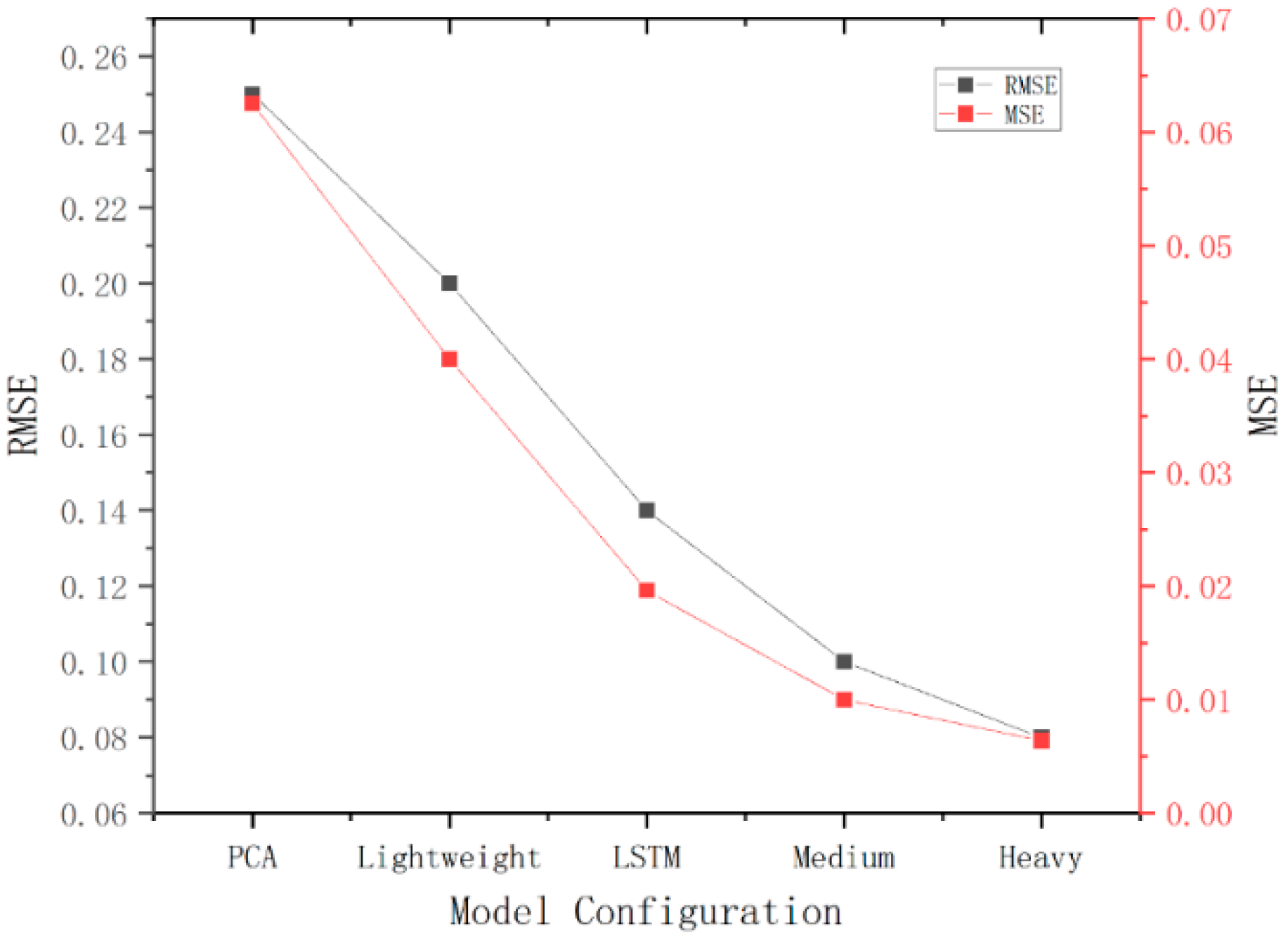
The network configuration and key hyperparameters used for model training are summarized in Table 3. A comparative analysis of reconstruction accuracy is presented in Figure 6 and Figure 7, where RMSE and MSE values are computed as the mean errors across five primary trajectory dimensions—East, North, altitude, ground speed, and heading angle—covering both spatial and kinematic fidelity. The results show that the Transformer–VAE consistently outperforms principal component analysis (PCA) and LSTM-based autoencoders, indicating its superior ability to extract compact representations while maintaining spatiotemporal structure.

3.5.1. Latent Space Visualization and Discrimination Analysis

To examine the structural distribution and class separability of the learned representations, the t-distributed Stochastic Neighbor Embedding (t-SNE) algorithm was employed to project 16-dimensional latent vectors into a two-dimensional space. The latent features were derived from the Transformer–VAE encoder after training on standardized trajectory inputs.
For the sake of reproducibility and interpretability, the Barnes–Hut implementation of t-SNE was adopted using a consistent set of stable parameters: perplexity = 30, learning rate = 200, 1000 iterations, Euclidean distance metric, and PCA initialization with a fixed random seed. These configurations are appropriate for the current dataset size—comprising several thousand trajectories—and they produce stable local neighborhood structures without excessive clustering.
It is important to note that t-SNE primarily preserves local similarity relationships rather than global metric distances. Consequently, the generated visualizations are used for qualitative analysis of the latent embedding space—for example, assessing the compactness and separation between arrival and departure trajectories, or comparing the distributions before and after joint optimization—rather than for quantitative evaluation. To maintain consistency, all t-SNE visualizations presented in this study were generated using the same parameters and initialization settings.
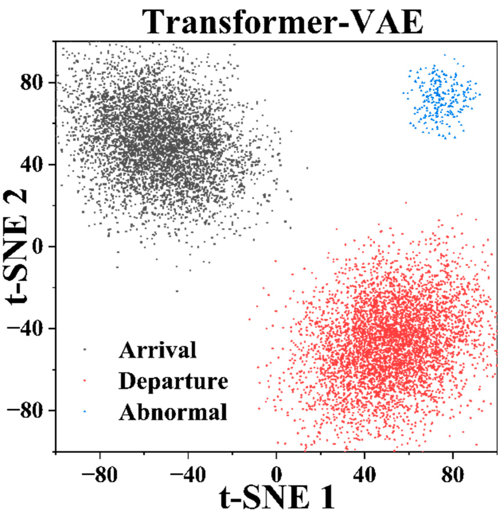
The resulting embedding is shown in Figure 8, where each point corresponds to a trajectory sample colored by its operational type (arrival, departure, or anomalous). The visualization reveals that arrival and departure trajectories form distinct clusters with compact intra-class alignment and clear inter-class separation. Low-density trajectories typically appear near the periphery, often lying between or outside the main clusters.
These results indicate that the latent space preserves the structural patterns of flight behaviors and exhibits meaningful separability, providing a solid basis for clustering and anomaly detection.

3.5.2. Comparison with Other Feature Extraction Models

To assess the comparative performance of representation methods, we benchmark the Transformer–VAE against Principal Component Analysis (PCA) and an LSTM-based Autoencoder (LSTM-AE). All models are trained on the same dataset, and their latent vectors are projected into two dimensions using t-SNE for visual inspection.
The embeddings are shown in Figure 9. PCA produces latent features with limited structural organization, resulting in substantial overlap between arrival and departure trajectories. LSTM-AE yields a more structured representation but still exhibits noticeable mixing between categories. By contrast, Transformer–VAE produces clearly separated clusters: arrivals and departures are grouped into distinct regions, while anomalous trajectories occupy a separate subspace.
This comparative analysis confirms that Transformer–VAE generates latent representations with stronger class separability, which is advantageous for downstream clustering and anomaly detection tasks.

3.6. Initial Cluster Center Extraction

After obtaining latent representations from the Transformer–VAE, initial clustering is performed using the Hierarchical Density-Based Spatial Clustering of Applications with Noise (HDBSCAN). As a density-based method, HDBSCAN does not require predefining the number of clusters and can adapt to variable-density distributions. The resulting partitions are used to compute mean latent vectors for each group, which serve as initialization for the subsequent joint optimization process described in Section 3.4.
The effectiveness of cluster initialization is further examined by comparing HDBSCAN with traditional strategies, including random initialization and K-means++ seeding. Figure 10 illustrates the latent space partitions obtained for both departure and arrival trajectories, while Table 4 summarizes the quantitative evaluation. The results show that HDBSCAN consistently achieves lower SSE, higher silhouette coefficients, and improved CH and DB scores relative to the baselines. Notably, the silhouette coefficient increases from 0.50 under random initialization to 0.65 under HDBSCAN, reflecting enhanced intra-cluster compactness and inter-cluster separability. These findings confirm that HDBSCAN provides a robust initialization strategy in latent spaces with heterogeneous density, thereby enabling more stable joint optimization in subsequent training.

3.7. Trajectory Clustering Results and Visualization

3.7.1. Clustering Results for Arrival Trajectories

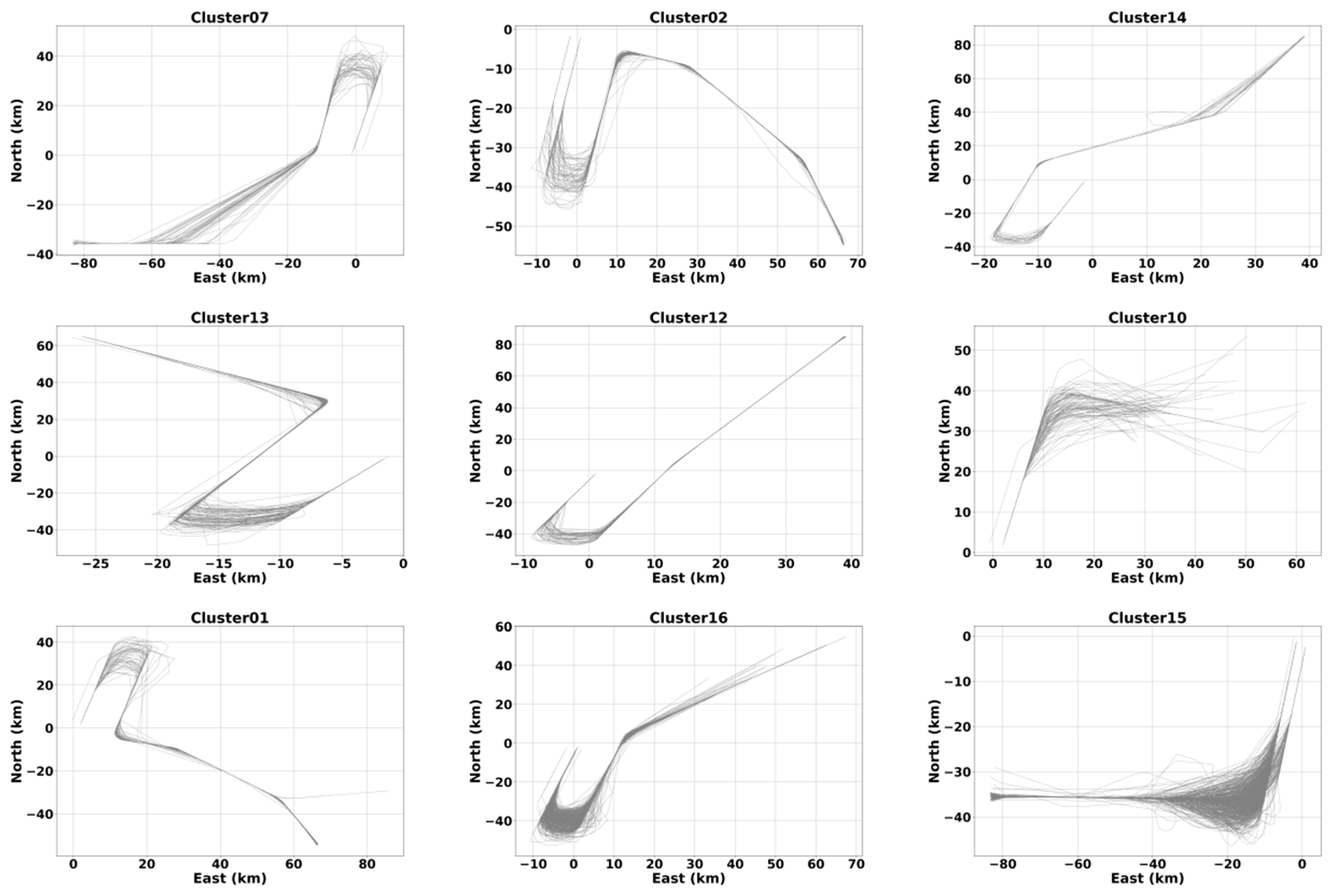
To evaluate the clustering performance for arrival operations, nine representative clusters were selected for visualization. For each cluster, a subset of trajectories was randomly sampled and projected onto the East–North–Up (ENU) plane to assess structural consistency and spatial separation. As shown in Figure 10, the Transformer–VAE-based framework effectively distinguishes diverse arrival patterns within the terminal area.
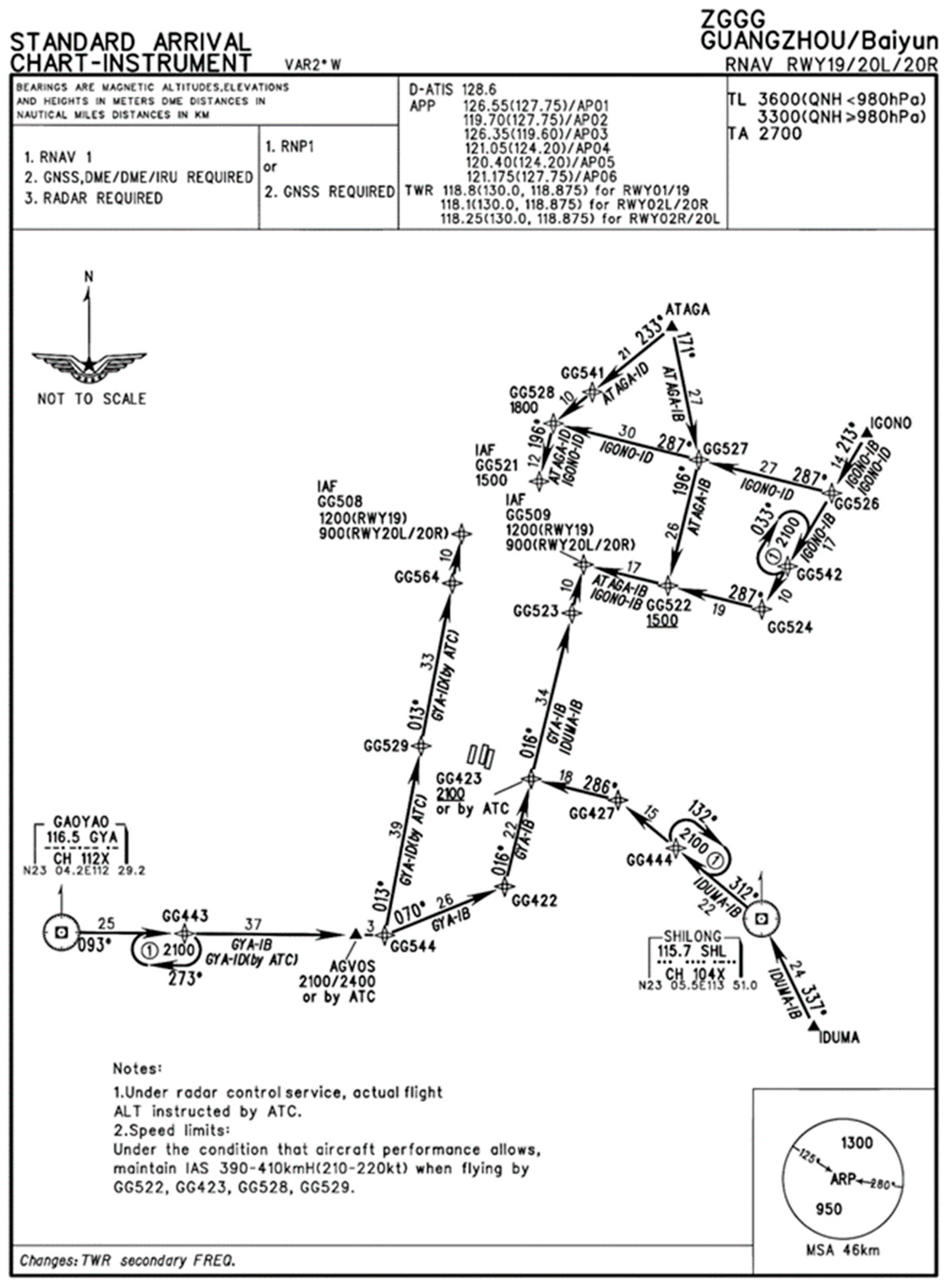
To provide spatial context, Figure 11 illustrates an illustrative Standard Terminal Arrival Route (STAR) chart for Guangzhou Baiyun International Airport.
This schematic chart is intended to provide a typical example of the arrival procedures in operation during 2018–2019.
Guangzhou Baiyun International Airport operates three runways—Runway 01/19 on the west side and two parallel runways 02L/20R and 02R/20L on the east side—with multiple approach directions serving both northern and southern entries to the terminal area.
The figure specifically depicts representative arrival flows toward Runways 19, 20L, and 20R, illustrating the converging inbound paths from different sectors.
The following cluster visualizations correspond to data-driven arrival patterns derived from ADS-B trajectories under these operational contexts.
The western 01/19 runway primarily handled single-runway operations, whereas the eastern pairs supported parallel approaches on 02L/02R and 20L/20R.
For readability, the horizontal and vertical scales of the subplots in Figure 12 differ slightly, but the relative orientations and trajectory patterns are preserved.
Overall, the clustered trajectories exhibit high intra-cluster compactness and clear inter-cluster separation, confirming the model’s ability to capture the geometric and operational diversity of terminal-area arrivals.
Northbound Arrivals (aligned with Runway 01 or 02L/02R)
Clusters 02, 13, 14, 12, 15, and 16 correspond to south-to-north arrivals primarily assigned to Runway 01 and the 02L/02R pair.
Clusters 13, 14, and 12 are clearly aligned with the single Runway 01:
Cluster 13 originates from the northwest, performs a ~90° right turn, briefly follows the runway direction, and then executes a ~180° left U-turn for final alignment—typical of curved turnaround approaches.
Cluster 14 approaches from the northeast, exhibits multiple small heading refinements (±10°) near characteristic arrival fixes, and ends with a left U-turn into final.
Cluster 12 represents a standardized straight-in descent from the northeast with minimal lateral deviation.
The remaining Clusters 02, 15, and 16 correspond to approaches toward the eastern 02L/02R runways:
Cluster 02 originates from the east–southeast, performing a wide right-turn convergence toward the parallel runways.
Cluster 15 approaches from the west, maintains a long straight segment, and shows a mild northeastward correction before aligning northbound.
Cluster 16 also enters from the northeast but includes intermediate merging and turning adjustments, reflecting more complex converging behavior.
Southbound Arrivals (aligned with Runway 20L/20R)
Clusters 01, 07, and 10 correspond to north-to-south arrivals assigned mainly to the 20L/20R runways.
Cluster 07 approaches from the southwest and achieves terminal alignment via a right-hand turn into a southbound final.
Cluster 01 originates from the east, showing small heading refinements near fix points—a ~90° right turn followed by a ~180° left U-turn for final alignment.
Cluster 10 enters from the northeast, featuring a smooth, broad left-hand descending curve into the final approach path.
Overall, the proposed method achieves compact intra-cluster consistency and distinct inter-cluster separation in terminal-area arrival flows.
The spatial structures identified by the Transformer–VAE framework are consistent with the three-runway layout and standard arrival (STAR) procedures at Guangzhou Baiyun International Airport, validating its utility for route classification, procedure evaluation, and airspace-structure monitoring.

3.7.2. Clustering Results for Departure Trajectories

As described in Section 3.7.1, Guangzhou Baiyun International Airport operated a three-runway configuration during 2018–2019.
In this section, the clustering results for departure operations are analyzed under the same spatial framework.
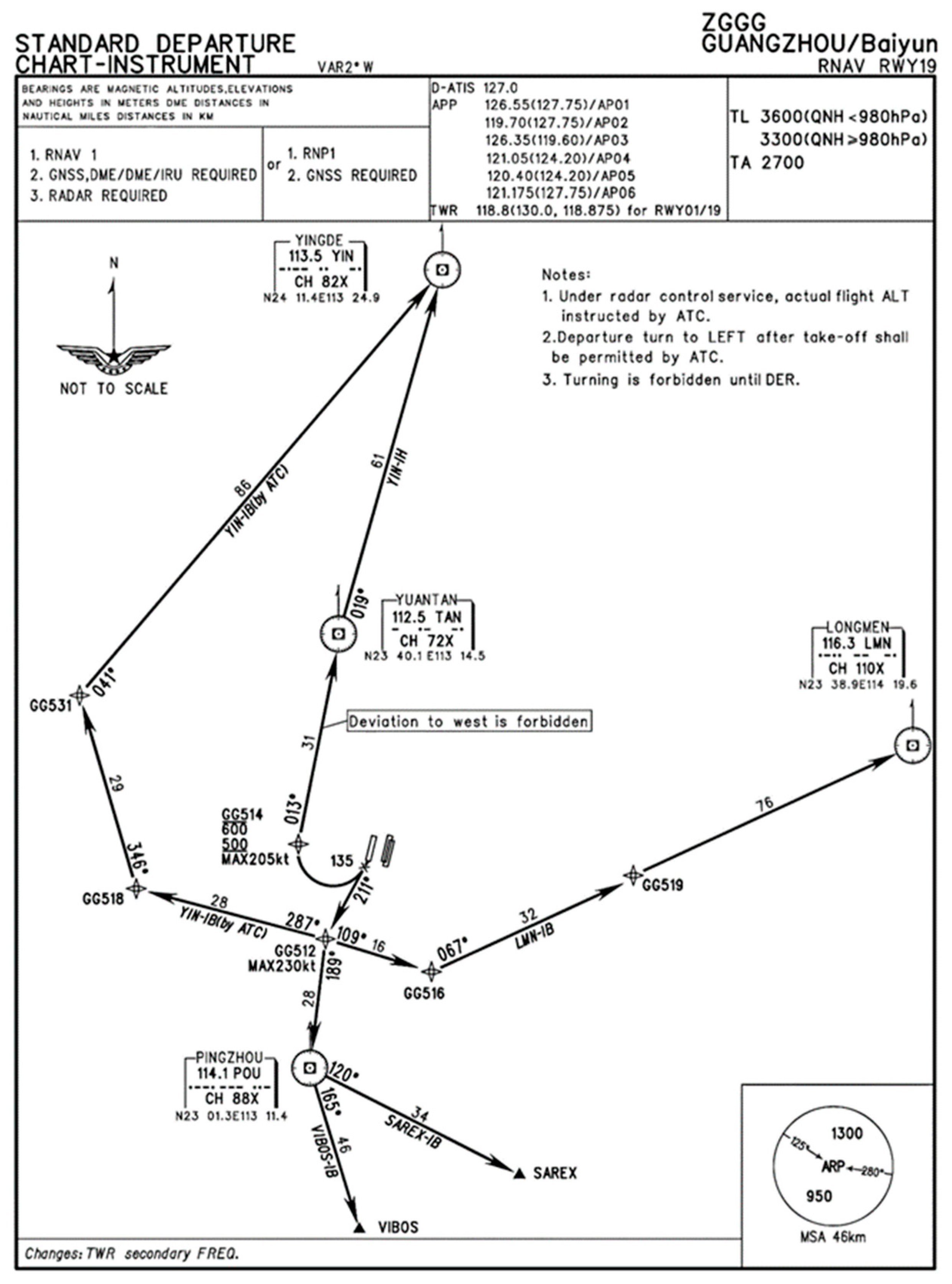
To enhance interpretability, Figure 13 presents a representative Standard Instrument Departure (SID) chart for Guangzhou Baiyun International Airport. This schematic example depicts the primary outbound direction and standard turning points for departures from Runway 01 during 2018–2019.
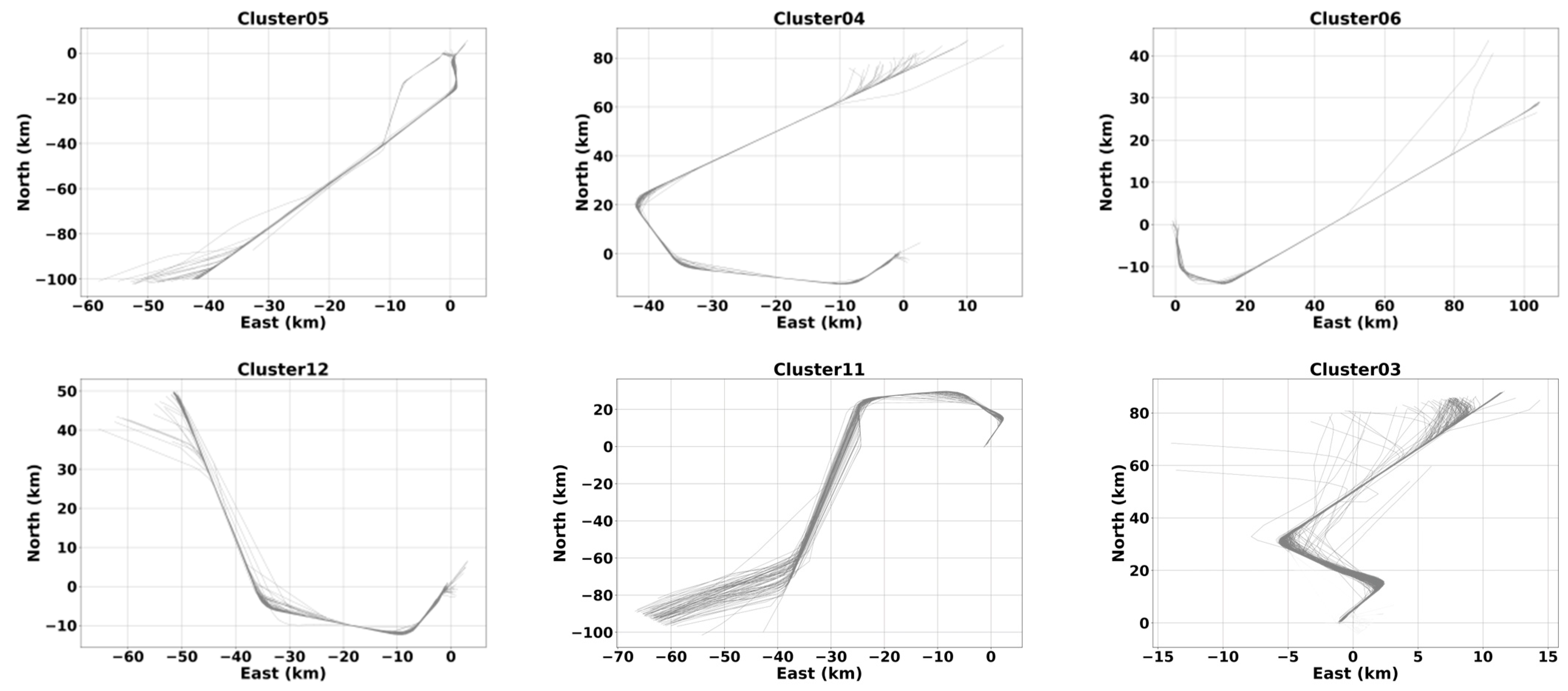
Nine representative clusters were selected for visualization. For each cluster, a subset of trajectories was randomly sampled and projected onto the East–North–Up (ENU) plane to examine the internal consistency and inter-cluster separability.
As illustrated in Figure 14, the Transformer–VAE-based framework effectively identifies multiple representative departure structures with clear directional patterns and compact cluster formations. For readability, the horizontal and vertical scales of the subplots in Figure 14 differ slightly, but the relative directions and geometric patterns are preserved for each cluster.
Northbound Departures (Runway 02L/02R).
Clusters 02, 03, 09, 11, and 12 correspond to northbound departures primarily taking off from Runways 02L/02R, exhibiting diverse geometric shapes while maintaining strong intra-cluster coherence.
Cluster 02 represents a standard northbound takeoff with a smooth right-hand turn toward the northeast, forming a stable and compact corridor.
Cluster 03 shows a left-turn maneuver after takeoff, transitioning from north to northwest heading, consistent with routes toward northern and northwestern China.
Cluster 09 initiates eastward and then performs a gentle right turn toward the southeast, delineating an eastbound outbound path.
Cluster 11 demonstrates a curved left-turn structure, evolving from northeast to northwest direction, indicating merging toward the northwestern exit point.
Cluster 12 executes a right-turn climb after takeoff, aligning with the northeastern outbound route, with highly consistent trajectories within the cluster.
These northbound patterns highlight the model’s capability to distinguish structured directional divergences in parallel runway departures.
Southbound Departures (Runway 19/20L/20R).
Clusters 01, 04, 05, and 06 represent southbound or southwest-bound departures, mainly operating on Runways 19 or 20L/20R.
Cluster 01 departs southeastward and then performs a left-turn toward the northeast, forming an “L”-shaped trajectory, typically associated with flights toward East Asia and coastal destinations.
Cluster 04 conducts a large right-turn maneuver in the southeastern sector, transitioning from east to southwest headings, typical of long-haul or southern domestic routes.
Cluster 05 climbs southward and then performs a broad left turn toward the southeast, maintaining high internal consistency and reflecting a stable southbound corridor.
Cluster 06 maintains a southbound climb, followed by a right turn into the southwest corridor, consistent with westbound or inland departures.
Overall, the proposed Transformer–VAE-based clustering framework achieves a high degree of intra-cluster compactness and clear inter-cluster separation for departure operations.
The clustered structures align well with the Standard Instrument Departure (SID) procedures of Guangzhou Baiyun International Airport and accurately reflect the organized flow of northbound and southbound departures under multi-runway operation.
These results confirm the effectiveness of the proposed method for route pattern recognition, airspace flow analysis, and departure flow management in complex terminal environments.

3.8. Effectiveness of Joint Optimization

In addition to the qualitative assessments in Section 3.5, a quantitative evaluation is conducted to examine the impact of the joint optimization strategy, which integrates Transformer–VAE-based representation learning with density-aware clustering to refine latent space structure. The analysis consists of three components.
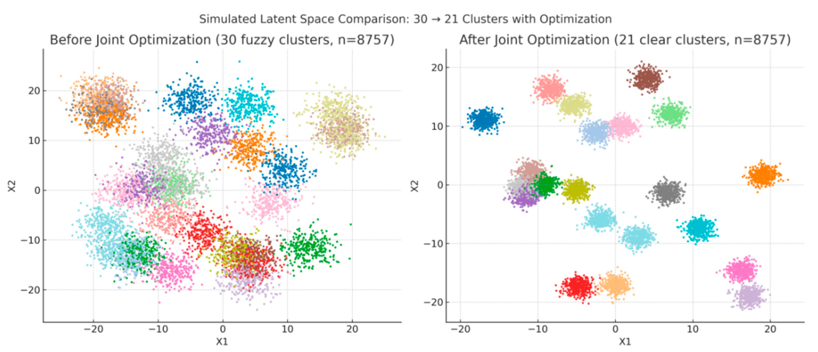
The effectiveness of joint optimization was first examined through quantitative evaluation. Table 5 summarizes clustering performance before and after optimization using four standard metrics: Sum of Squared Errors (SSE), Silhouette Coefficient (SC), Calinski–Harabasz Index (CH), and Davies–Bouldin Index (DB). The results indicate a substantial reduction in SSE and DB, accompanied by notable improvements in SC and CH, which together demonstrate enhanced intra-cluster compactness and inter-cluster separability.
To further assess structural changes, two-dimensional t-SNE projections of the latent embeddings are shown in Figure 15. Prior to optimization, the embedding distribution is diffuse, with substantial overlap between clusters. After optimization, clusters become more compact with clearer boundaries, reflecting improved separability in the latent space.
Training dynamics were also monitored by tracking the Kullback–Leibler divergence between the soft assignment distribution and the target distribution. As shown in Figure 16, the KL loss decreases rapidly within the first 80 epochs and then stabilizes, suggesting that the latent space converges to a consistent clustering configuration.

3.9. Computational Efficiency and Large-Scale Evaluation

To ensure practical applicability in large-scale trajectory processing, the proposed framework incorporates optimizations in segmentation, representation learning, and clustering with emphasis on runtime and memory efficiency. The evaluation is conducted on a real-world ADS-B dataset consisting of approximately 27,759 terminal-area trajectories and more than 3.0 million data points.
In the segmentation stage, the DFE-MDL algorithm adaptively selects key points based on speed and heading rate variations, reducing the number of retained points while maintaining reconstruction fidelity. This reduces average segmentation time from 95 ms to 28 ms per trajectory, corresponding to a 72.4% improvement under comparable accuracy (Table 6).
In subsequent stages, the Transformer–VAE employs a lightweight symmetric encoder–decoder architecture (four layers, latent dimension 16–64) to accelerate training, while HDBSCAN is used for cluster initialization to avoid redundant computations and manual parameter tuning.
The complete pipeline—including preprocessing, segmentation, feature extraction, and clustering—was executed under the same hardware environment described in Section 3.2. The average per-trajectory processing time decreased from 122 ms to 55 ms after optimization, enabling the full dataset to be processed in approximately 1.389 s.
These results confirm that the proposed framework achieves substantial runtime reductions while maintaining or improving clustering quality. The observed efficiency gains highlight its computational feasibility for high-volume trajectory analysis under standard workstation configurations.

4. Conclusions and Future Works

This study proposed a unified framework for trajectory clustering in terminal airspace, integrating dynamics-aware segmentation, Transformer–VAE-based representation learning, and density-aware clustering with joint optimization. The DFE-MDL segmentation effectively preserved maneuver boundaries and reduced reconstruction errors, while the Transformer–VAE encoder generated compact latent embeddings with clear separability. Initialization with HDBSCAN and refinement through KL divergence further improved clustering performance, as confirmed by consistent gains across SSE, SC, CH, and DB metrics. Experiments on large-scale ADS-B data from Guangzhou Baiyun International Airport demonstrated that the framework achieves both accuracy and computational efficiency, producing interpretable flow structures that support STAR/SID compliance monitoring, flow discovery, and anomaly detection.
One avenue for future research is to extend the framework with contextual factors such as weather and ATC interventions to enhance robustness in operational environments. Another is to develop online or adaptive variants that enable real-time clustering in dynamic terminal areas. It would also be interesting to integrate explainability mechanisms to improve transparency and support practical adoption in air traffic management.

Author Contributions

Conceptualization, Q.C.; methodology, Q.C.; coding, Q.C.; validation, Q.C.; investigation, Q.C.; resources, M.L.; data curation, Q.C.; writing—original draft preparation, Q.C.; writing—review and editing, M.L.; visualization, Q.C.; supervision, M.L.; funding acquisition, M.L. All authors have read and agreed to the published version of the manuscript.

Funding

This work was supported in part by the Jiangsu Provincial Natural Science Foundation [BK20151479] and the Humanities and Social Science Fund of the Ministry of Education [Grant 23YJC790027].

Data Availability Statement

Data will be made available on request.

Conflicts of Interest

The authors declare no conflicts of interest.

Abbreviations

TMAs Terminal Maneuvering Areas
ATM Air Traffic Management
TBO Trajectory Based Operations
ATOP Aircraft Trajectory Optimization Problem
t-SNEt-Distributed Stochastic Neighbor Embedding
HDBSCANHierarchical Density-based Spatial Clustering of Applications with Noise
VAEVariational Autoencoder

References

  1. ICAO. Annual Safety Report 2023; ICAO: Montreal, QC, Canada, 2023. [Google Scholar]
  2. Eurocontrol. Challenges of Growth 2018—Summary Report; Eurocontrol: Brussels, Belgium, 2018. [Google Scholar]
  3. SESAR Joint Undertaking. European ATM Master Plan—Digitalising Europe’s Aviation Infrastructure; SESAR JU: Brussels, Belgium, 2020. [Google Scholar]
  4. ICAO. Global Air Navigation Plan 2022–2038; ICAO: Montreal, QC, Canada, 2022. [Google Scholar]
  5. Olive, X.; Basora, L.; Delahaye, D. Deep learning for aircraft trajectory clustering: An enabler for traffic complexity analysis. Transp. Res. Part C Emerg. Technol. 2023, 147, 103956. [Google Scholar] [CrossRef]
  6. Wang, S.; Wu, Y.; Wang, Y. Deep spatiotemporal trajectory representation learning for clustering. IEEE Trans. Intell. Transp. Syst. 2024, 25, 7687–7700. [Google Scholar] [CrossRef]
  7. Lee, J.G.; Han, J.; Whang, K.Y. Trajectory clustering: A partition-and-group framework. In Proceedings of the 2007 ACM SIGMOD International Conference on Management of Data, Beijing, China, 11–14 June 2007; pp. 593–604. [Google Scholar] [CrossRef]
  8. Li, Z.; Ding, B.; Han, J.; Kays, R.; Nye, P. Mining periodic behaviors for moving objects. In Proceedings of the 16th ACM SIGKDD International Conference on Knowledge Discovery and Data Mining, Washington, DC, USA, 24–28 July 2010; pp. 1099–1108. [Google Scholar] [CrossRef]
  9. Mahboubi, H.; Miller, N.; Kamgarpour, M. Trajectory Clustering with Application to Air Traffic. In AIAA Scitech 2021 Forum; AIAA: Reston, VA, USA, 2021. [Google Scholar] [CrossRef]
  10. Bolić, T.; Pantazis, A.; Reyes, L. Trajectory clustering for air traffic categorisation. Aerospace 2022, 9, 227. [Google Scholar] [CrossRef]
  11. Hao, J.-Y.; Xu, C.; Fan, R.; Li, S.; Zhang, T. Trajectory clustering based on length-scale directive Hausdorff. In Proceedings of the 16th International IEEE Conference on Intelligent Transportation Systems (ITSC 2013), The Hague, The Netherlands, 6–9 October 2013; pp. 1300–1305. [Google Scholar] [CrossRef]
  12. Hinton, G.E.; Salakhutdinov, R.R. Reducing the dimensionality of data with neural networks. Science 2006, 313, 504–507. [Google Scholar] [CrossRef]
  13. Kingma, D.P.; Welling, M. Auto-encoding variational Bayes. arXiv 2014. [CrossRef]
  14. Vaswani, A.; Shazeer, N.; Parmar, N.; Uszkoreit, J.; Jones, L.; Gomez, A.N.; Kaiser, L.; Polosukhin, I. Attention is all you need. Adv. Neural Inf. Process. Syst. 2017, 30, 5998–6008. [Google Scholar]
  15. Zhang, W.; Hu, M.; Du, J. An end-to-end framework for flight trajectory data analysis based on deep autoencoder network. Aerosp. Sci. Technol. 2022, 123, 107726. [Google Scholar] [CrossRef]
  16. Liu, Y.; Ng, K.H.; Chu, N.; Hon, K.K.; Zhang, X. Spatiotemporal image-based flight trajectory clustering model with deep convolutional autoencoder network. J. Aerosp. Inf. Syst. 2023, 20, 234–247. [Google Scholar] [CrossRef]
  17. Postnikov, A.; Gamayunov, A.; Ferrer, G. Transformer-based trajectory prediction. arXiv 2021, arXiv:2112.04350. [Google Scholar] [CrossRef]
  18. Nogueira, T.P.; Braga, R.B.; Oliveira, C.T.; Martin, H. FrameSTEP: A framework for annotating semantic trajectories based on episodes. Expert Syst. Appl. 2018, 92, 533–545. [Google Scholar] [CrossRef]
  19. Cao, H.; Mamoulis, N.; Cheung, D.W. Discovery of periodic patterns in spatiotemporal sequences. IEEE Trans. Knowl. Data Eng. 2007, 19, 453–467. [Google Scholar] [CrossRef]
  20. Hu, D.; Chen, L.; Fang, H.; Fang, Z.; Li, T.; Gao, Y. Spatio-temporal trajectory similarity measures: A comprehensive survey and quantitative study. IEEE Trans. Knowl. Data Eng. 2024, 36, 2191–2212. [Google Scholar] [CrossRef]
  21. Fang, Z.; Du, Y.; Zhu, X.; Hu, D.; Chen, L.; Gao, Y.; Jensen, C.S. Spatio-temporal trajectory similarity learning in road networks. In Proceedings of the 28th ACM SIGKDD Conference on Knowledge Discovery and Data Mining, Washington, DC, USA, 14–18 August 2022; pp. 347– 356. [Google Scholar] [CrossRef]
  22. Li, L.; Si, J.; Lv, J.; Lu, J.; Zhang, J.; Dai, S. MSST: Multi-scale spatial-temporal representation learning for trajectory similarity computation. IEEE Trans. Big Data 2025, 11, 2657–2668. [Google Scholar] [CrossRef]
  23. Su, H.; Liu, S.; Zheng, B.; Zhou, X.; Zheng, K. A survey of trajectory distance measures and performance evaluation. VLDB J. 2020, 29, 3–32. [Google Scholar] [CrossRef]
  24. Liang, A.; Yao, B.; Wang, B.; Liu, Y.; Chen, Z.; Xie, J.; Li, F. Sub-trajectory clustering with deep reinforcement learning. VLDB J. 2024, Online First. [Google Scholar] [CrossRef]
  25. Zeng, W.; Guo, X.; Chen, W.; Zhang, R.; Liu, P. Aircraft trajectory clustering in terminal airspace based on deep autoencoder and Gaussian mixture model. Aerosp. Sci. Technol. 2022, 122, 107674. [Google Scholar] [CrossRef]
  26. Barratt, S.T.; Kochenderfer, M.J.; Boyd, S.P. Learning probabilistic trajectory models of aircraft in terminal airspace from position data. IEEE Trans. Intell. Transp. Syst. 2019, 20, 3536–3545. [Google Scholar] [CrossRef]
  27. Bombelli, A.; Soler, L.; Trumbauer, E.; Mease, K.D. Strategic air traffic planning with Fréchet distance aggregation and rerouting. J. Guid. Control Dyn. 2017, 40, 700–711. [Google Scholar] [CrossRef]
  28. Zhang, W.; Payan, A.; Mavris, D.N. Air traffic flow identification and recognition in terminal airspace through machine learning approaches. In Proceedings of the AIAA Scitech 2024 Forum, Orlando, FL, USA, 8–12 January 2024. Paper AIAA 2024-0536. [Google Scholar] [CrossRef]
  29. Paradis, C.; Davies, M.D. Visualizing corridors in terminal airspace using trajectory clustering. In Proceedings of the IEEE/AIAA 41st Digital Avionics Systems Conference (DASC), Portsmouth, VA, USA, 18–22 September 2022. [Google Scholar] [CrossRef]
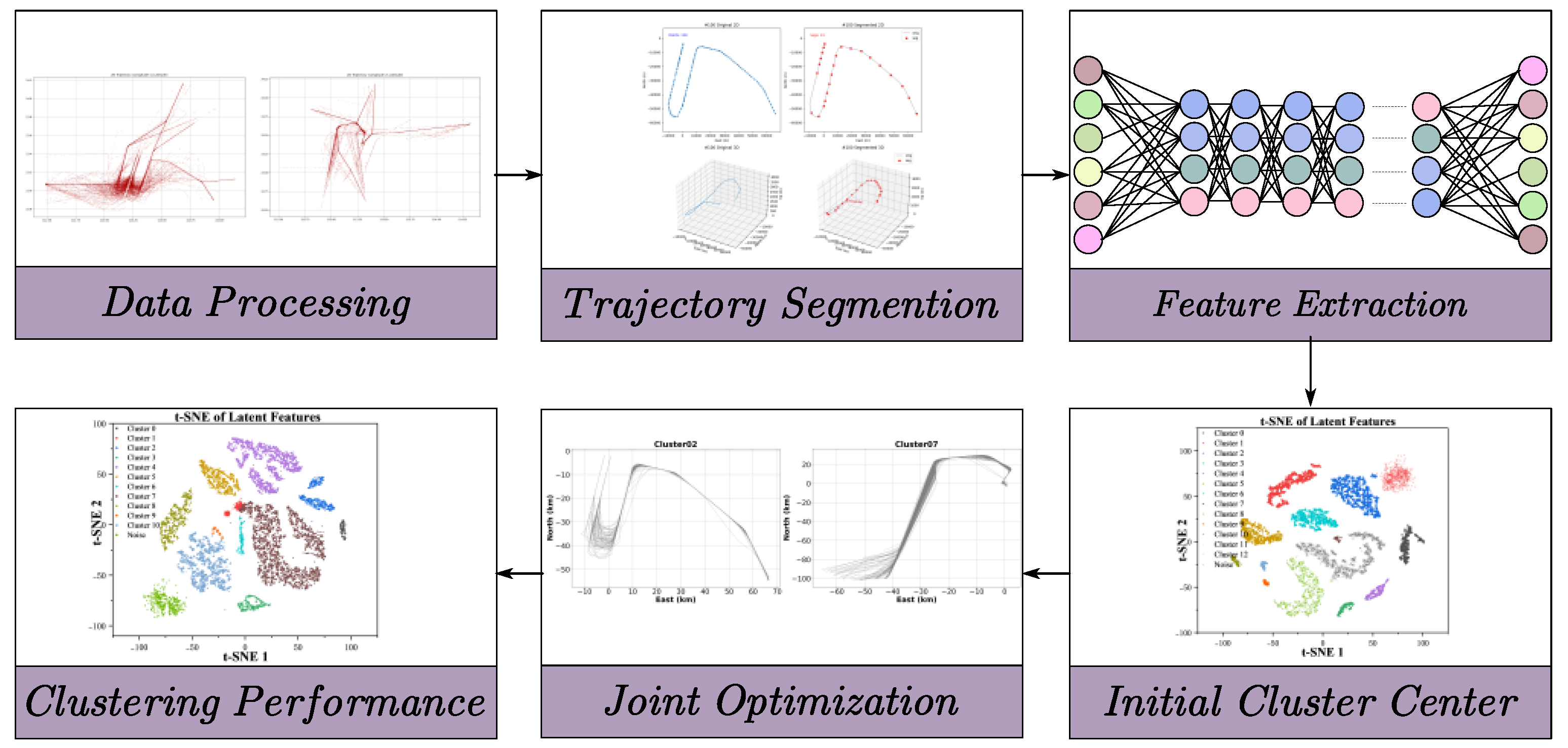
Figure 1. Overview of the proposed trajectory clustering framework.
Aerospace 12 00969 g001
Figure 2. Architecture of the Transformer–VAE network.
Aerospace 12 00969 g002
Figure 3. Trajectories in the ENU frame: (a) Departure trajectories in the ENU frame; (b) Arrival trajectories in the ENU frame.
Aerospace 12 00969 g003
Figure 4. Visual comparison of trajectory reconstructions with 25 uniformly retained points (≈10% of the original samples) across all methods.
Aerospace 12 00969 g004
Figure 5. Comparison of resampling strategies.
Aerospace 12 00969 g005
Figure 6. Overall reconstruction errors (RMSE and MSE) averaged across five key trajectory dimensions. “Light,” “Medium,” and “Heavy” correspond to different network configurations with hidden dimensions of 128, 256, and 512, respectively.
Aerospace 12 00969 g006
Figure 7. Reconstruction errors (RMSE and MSE) for different network configurations, averaged across the same five dimensions.
Aerospace 12 00969 g007
Figure 8. t-SNE Visualization of Latent Trajectory Embeddings by Flight Operation Type.
Aerospace 12 00969 g008
Figure 9. Comparison of Latent Feature Distributions via PCA, LSTM-AE, and Transformer–VAE.
Aerospace 12 00969 g009
Figure 10. Latent-space projections and HDBSCAN clustering for (left) departures and (right) arrivals.
Aerospace 12 00969 g010
Figure 11. Representative Standard Terminal Arrival Route (STAR) for Guangzhou Baiyun International Airport, illustrating the typical converging approach paths toward Runways 19, 20L and 20R.
Aerospace 12 00969 g011
Figure 12. Arrival Trajectory Clusters (9 Categories). Note that the scales of subplots are adjusted individually to reflect the actual spatial extent of trajectories (10–80 km).
Aerospace 12 00969 g012
Figure 13. Representative Standard Instrument Departure (SID) for Guangzhou Baiyun International Airport, showing the main outbound directions and turning points from Runways 01.
Aerospace 12 00969 g013
Figure 14. Departure Trajectory Clusters (9 Categories).
Aerospace 12 00969 g014aAerospace 12 00969 g014b
Figure 15. t-SNE projections of latent embeddings before (left) and after (right) joint optimization.
Aerospace 12 00969 g015
Figure 16. KL divergence convergence during joint optimization.
Aerospace 12 00969 g016
Table 1. Reconstruction accuracy under different segmentation algorithms.
MethodRMSEAPD
Uniform Sampling0.05710.0312
Douglas–Peucker0.04650.0251
Visvalingam–Whyatt0.04230.0215
DFE-MDL (proposed)0.02940.0187
Table 2. Trajectory reconstruction performance of Transformer–VAE across multiple feature dimensions.
DimensionsRMSEMAE
East (km)0.00180.0014
North (km)0.00150.0012
Altitude (m)22.618.2
Speed (kt)5.24.1
Heading angle (°)7.15.6
Table 3. Different network configuration parameters.
Model ParametersLightMedium
Hidden Dimensions128256
Number of Encoder and Decoder Layers24
Feedforward Network Dimension5121204
Table 4. Final clustering performance under different initialization strategies.
Initialization StrategySSESilhouette
Coefficient
Calinski-HarabaszDavies-Bouldin
Random520.40.5300.20.9
K-means++480.10.58350.70.72
HDBSCAN430.70.65410.90.55
Table 5. Clustering performance before and after joint optimization.
MetricBefore OptimizationAfter Optimization
SSE124,50083,200
Silhouette Coefficient0.310.48
Calinski–Harabasz43007950
Davies–Bouldin1.871.12
Table 6. Estimated per-trajectory processing time across core modules before and after optimization.
Module StageProcessing Time
(per Trajectory)
Before Optimization (Full Trajectory)After Optimization (Segmented + Filtered)
Trajectory Preprocessing~5 ms~5 msConstant
Segmentation ComputationAvg. 42 ms~95 msReduced to 28 ms
Feature Extraction (VAE)~22 msConstant
Clustering Initialization (HDBSCAN)~1.3 min (overall)Constant
Disclaimer/Publisher’s Note: The statements, opinions and data contained in all publications are solely those of the individual author(s) and contributor(s) and not of MDPI and/or the editor(s). MDPI and/or the editor(s) disclaim responsibility for any injury to people or property resulting from any ideas, methods, instructions or products referred to in the content.