Real-Time Aerodynamic Airfoil Optimisation Using Deep Reinforcement Learning with Proximal Policy Optimisation

Abstract

This research presents the application of Reinforcement Learning (RL) techniques to optimise aerodynamic profiles in real time, within the context of morphing wings. By implementing Proximal Policy Optimisation (PPO), a methodology has been developed that learns to satisfy both aerodynamic objectives and complex geometric constraints, such as internal spatial limitations or payload integration volumes. The approach achieves an effective balance between performance and constraint satisfaction while maintaining low computational cost and millisecond-level optimisation speed. A scalable tool has been developed for real-time optimisation in such contexts, with applications in adaptive design for both manned and unmanned aviation.

1. Introduction and State of the Art

Since the early days of aviation, continuous efforts have been made to design lighter and more efficient aircraft, achieving milestones unimaginable a century ago. Today, hundreds of passengers can cross oceans in a single flight at increasingly affordable costs. Commercial aviation even entered the supersonic era, which is expected to return soon with projects such as Boom Supersonic [1]. Military aviation, meanwhile, has produced highly manoeuvrable aircraft capable of exceeding twice the speed of sound and sustaining long missions thanks to engine efficiency.

The advances achieved are the result of the unprecedented efforts of the industry, largely driven by a branch of engineering dedicated to obtaining better results with fewer resources: optimisation.

In this research, Reinforcement Learning (RL) methods are applied for the optimisation of an airfoil design, considering both aerodynamic performance and explicit geometric constraints under specific boundary conditions.

Lampton et al. [2] apply the Q-Learning algorithm to a 2D morphing wing, providing degrees of freedom such as the airfoil thickness, camber, maximum camber position, and angle of attack. Additionally, they discretise the states and actions so that the algorithm can work with them. They achieve this by creating a grid of values in the continuous space. The study demonstrates that a larger state step (profile variation) at each stage leads to faster convergence, though this may result in less detailed exploration. Furthermore, after conducting a balance analysis between exploration and exploitation, it is observed that starting with dominant exploration and progressively shifting towards greater exploitation is the most effective approach.

On the other hand, Chen et al. [3] use the Deep Deterministic Policy Gradient (DDPG) algorithm to optimise the surface of aerodynamic profiles, successfully eliminating transonic buffet, a phenomenon that causes large self-excited oscillations of the shockwave on the wing surface, triggered by the interaction between the shockwaves and the boundary layer. Jiang et al. [4] apply the algorithm to a variable-sweep morphing wing, adding a Long Short-Term Memory (LSTM) network, resulting in a DDPG with a Task Classifier. This approach allows the LSTM to classify the phase in which the aircraft is, enabling the strategy to change depending on the detected flight phase. The new approach has led to more efficient training and more robust results, with a reward up to 75% higher than with DDPG. Yan et al. [5] use DDPG to optimise the geometry of missile fins with the aim of maximising cruising efficiency, having to meet constraints such as the position of the centre of pressure or a maximum drag coefficient (CD). Additionally, they innovate by introducing Transfer Learning in the agent’s training, allowing an agent to be retrained in a new environment. This is used in their research to carry out initial training with the semi-empirical software DATCOM, which allows general knowledge to be acquired, before later using neural networks in new training conducted with CFD, which enables greater precision. In this way, a less computationally expensive environment is used in the early stages, before finally employing a more accurate but considerably slower environment.

Dussauge et al. [6] use the Proximal Policy Optimisation (PPO) algorithm for the design of optimised aerodynamic profiles, exploring different parameterisation methods and action spaces, which will be addressed later. They conclude that, compared to other algorithms such as gradient-based ones, the learning is more efficient, and it is also capable of learning a policy that can be applied to new cases. Hui et al. [7] also investigate the optimisation of profiles using PPO. To do so, they propose a Pareto optimisation approach, where the profile must maximise its efficiency under two different flight conditions, while meeting a dimensional constraint of not reducing its thickness. After their analysis, they indicate that it required 15% of the time that a genetic algorithm would need for the same task, achieving between 4.3% and 10.1% better results than the base profile. Viquerat et al. [8] optimise profiles using a degenerate DRL approach, which consists of achieving their goal in just one step, unlike other cases where each episode consists of numerous steps. Li et al. [9] carry out the optimisation seeking to reduce the CD, and to increase the efficiency of model creation, they first perform pretraining using Imitation Learning, a technique that allows the model to be trained with high-quality action-state samples obtained through other methods, such as human experience. In this way, the training is guided more effectively.

Finally, Bruin et al. [10] propose starting the model training with gradient-based optimisation, as is commonly done in DRL algorithms, and at a later stage switching to gradient-free optimisation. In this way, the effectiveness of the former is combined with the stability and convergence capability of the latter. Results are achieved that would not be possible with gradient-based optimisation alone, requiring far fewer iterations than an evolutionary algorithm like CMA-ES, one of the most advanced algorithms.

The novelty of our research lies in the design of a reinforcement learning methodology capable of optimising airfoil geometries while simultaneously satisfying user-defined aerodynamic and geometric constraints. Unlike previous works focused on unconstrained optimisation, the proposed framework explicitly accounts for internal spatial limitations, enabling designs that respect predefined integration or payload volumes. The method operates in a quasi-real-time environment, computing morphing-wing geometries within milliseconds and demonstrating the feasibility of applying DRL to constrained aerodynamic design. To evaluate the approach, a software tool, DRLFoil v0.1.0, has been developed, allowing users to obtain optimised profiles that meet design constraints almost in real time. The developed tool, named DRLFoil, can be found with its respective user guide at https://github.com/DRL-Geometry-Optimization/DRLFoil.git (accessed on 15 August 2025).

The structure of the document is as follows: Section 2 describes the technological background used for the development of the methodology, a schematic of the idea behind the methodology, and the necessary algorithms are elaborated. Section 3 shows the results obtained with the tool developed to test the methodology, and Section 4 concludes with the outcomes.

2. Materials and Methods

2.1. Deep Reinforcement Learning Algorithm

Machine Learning, and specifically Deep Learning, has marked a significant advancement in the development of AI and modern technology. However, one of its greatest limitations stems from its nature: its ability to generate outputs depends on the training data it has received, preventing it from discovering new possibilities. The need to find solutions without relying on external data has been addressed through Reinforcement Learning.

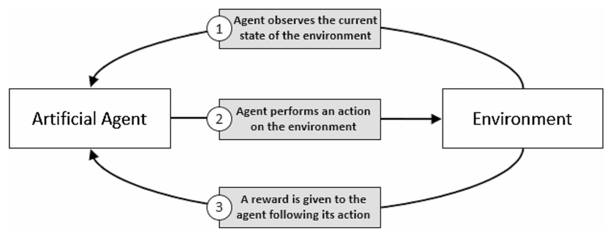
Reinforcement Learning consists of a learning process that seeks to maximise a numerical reward signal. This is achieved through the interaction of an intelligent agent with an environment, as shown in Figure 1. Unlike other methods, the agent does not receive explicit instructions on which actions to take but must discover them through trial and error. Additionally, the actions consider not only the immediate reward but also future rewards that may be received based on the action taken.

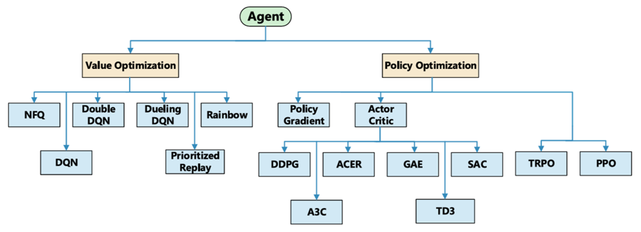
The growth of current needs, especially with the emergence of higher-dimensional states and actions, has rendered existing algorithms incapable of meeting the proposed requirements. One of the most widely used and successful options has been the use of DL as approximation functions. This is how Deep Reinforcement Learning (DRL) emerged, and it has been responsible for most advances in this field. Some of the most important DRL algorithms can be seen in Figure 2.

2.1.1. Agent

The algorithm governing the RL agent will be implemented using the open-source library Stable Baselines 3 (SB3) [12]. This has been developed using PyTorch v2.3.0 and is based on the OpenAI Baselines library. Its development focuses on providing reliable and reproducible implementations of the algorithms, ensuring that the performance obtained is stable and preventing a small user difference in the implementation from significantly affecting the results. Additionally, it includes automated unit tests that cover 95% of the code, thus avoiding development errors that could occur if the algorithms were created by the user [13].

The algorithms implemented by SB3 are numerous, including Stable Baselines3 Contrib, DDPG, and PPO, as well as DQN and Recurrent Proximal Policy Optimisation (RecurrentPPO).

Table 1. Action spaces and multithreading support for some of the SB3 algorithms [12].

Name	Box	Discrete	MultiDiscrete	MultiBinary	Multiprocessing
PPO	Yes	Yes	Yes	Yes	Yes
DDPG	Yes	No	No	No	Yes
DQN	No	Yes	No	No	Yes
RecurrentPPO	Yes	Yes	Yes	Yes	Yes

shows the capabilities of each implementation to support different action spaces. Box is an N-dimensional space that contains all possible points in the action space. Discrete refers to a list of actions where only one can be used at each time step. MultiDiscrete consists of a list of sets of discrete actions, allowing one action from each set to be used at each time step. Finally, MultiBinary is a list of possible actions where any combination of these actions can be used at each time step.

The algorithm selected for the aerodynamic optimisation of DRLFoil is PPO. This is due to the simplicity of its hyperparameters, which allows for easier optimisation compared to DDPG, and particularly because of its ability to support continuous action spaces, which DQN does not allow. Additionally, its design provides more stable implementation than DDPG and is less prone to deviations during training, which is crucial in complex applications such as aerodynamic optimisation. On the other hand, the option of Recurrent-PPO has been discarded as it is an experimental version, although its future use may be relevant due to its ability to handle temporal dependencies, which is ideal for real-time optimisation like morphing wings, among other features.

2.1.2. Environment

In this case, Gymnasium [14] has been used, an API that continues the OpenAI Gym project and provides standards for the development of environments and the subsequent use and evaluation of RL algorithms. In this way, since common methods are provided for all environments developed on this platform, as well as full compatibility of SB3 with Gymnasium, developing the environment based on this library is particularly straightforward.

When selecting an aerodynamic analysis method, a balance must be struck between the project’s requirements, the results expected, and the computational and time resources available. In our case, we have decided to prioritise minimising training and inference times for several reasons: firstly, because we seek to obtain results quickly to avoid unnecessary resource expenditures; secondly, it has been considered that there are numerous analysis resources that are sufficiently accurate with considerably lower analysis times compared to methods such as CFD; thirdly, achieving very low inference times opens the door to real-time and onboard optimisations in aircraft, such as in the case of morphing wings or even other systems like flight control using DRL.

In this way, the method that offered the shortest calculation time while maintaining acceptable results is NeuralFoil [15], a tool consisting of a PINN trained with millions of profiles in XFOIL. As shown in

Table 2. Comparison of different model sizes of NeuralFoil with XFOIL [15].

Model	CL MAE	CD MAE	CM MAE	Time (1 Execution)
NF “medium”	0.02	0.039	0.003	5 ms
NF “large”	0.016	0.03	0.003	8 ms
NF “xlarge”	0.013	0.024	0.002	13 ms
NF “xxlarge”	0.012	0.022	0.002	16 ms
NF “xxxlarge”	0.012	0.02	0.002	56 ms
XFOIL	0	0	0	73 ms

and graphically in Figure 3, the accuracy of NeuralFoil is high compared to the training data, achieving inference times of around five milliseconds.

The tool can calculate both CL and CD on Reynolds numbers from 10² to 10¹⁰. The developer warns that larger models tend to show greater oscillations in the results due to the high number of parameters in the model, which can complicate the learning process [16]. For this reason, the “xlarge” model will be used throughout this project.

NeuralFoil is implemented within AeroSandbox [17], a package by the same author that includes tools to facilitate working with aerodynamic profiles. Using this tool, the CST parameterisation will be used to characterise the profiles, as it is directly compatible with NeuralFoil’s operation.

The Class-Shape Transformation (CST) parameterisation is the most widely used method in aerodynamic profile optimisation. It is a method designed to obtain these shapes in a simple way and is especially useful in optimising geometries. Among the advantages it offers compared to other methods is the existence of an infinite slope at the leading edge, which allows for a rounded edge, as well as a finite trailing edge [18].

$$\mathsf{\zeta }\left(\mathsf{\psi }\right)=C\left(\mathsf{\psi }\right)S\left(\mathsf{\psi }\right)$$

(1)

where $\mathsf{\psi }={\displaystyle \frac{x}{c}} \mathrm{and}\mathsf{\zeta }={\displaystyle \frac{z}{c}}$. The class function for the upper and lower coordinates of the aerodynamic profile is defined as:

$$C\left(\mathsf{\psi }\right)={\mathsf{\psi }}^{N_1}{\left(1-\mathsf{\psi }\right)}^{{ N}_2}$$

(2)

${\mathrm{N}}_1=0.5$ ensures a rounded leading edge with an infinite slope at $\mathsf{\psi }=0$. To achieve a finite trailing edge angle at $\mathsf{\psi }=1$, ${\mathrm{N}}_2$ is set as ${\mathrm{N}}_2=1$. S Bernstein polynomials are used as weighted shape functions. The weighting factors ${\mathrm{x}}_{\mathrm{i}}$ are the design variables for the optimisation.

$$\mathrm{S}\left(\mathsf{\psi }\right)={\displaystyle \sum _{\mathrm{i}=0}^{\mathrm{n}}}{\mathrm{x}}_{\mathrm{i}}{\mathrm{B}}_{\mathrm{i}}\left(\mathsf{\psi }\right)$$

(3)

where

$${\mathrm{B}}_{\mathrm{i}}\left(\mathsf{\psi }\right)={\mathrm{K}}_{\mathrm{i}}{\mathsf{\psi }}^{\mathrm{i}}{\left(1-\mathsf{\psi }\right)}^{ \mathrm{n}-\mathrm{i}}$$

(4)

$${\mathrm{K}}_{\mathrm{i}}=\left({\displaystyle \genfrac{}{}{0pt}{}{\mathrm{n}}{\mathrm{i}}}\right)={\displaystyle \frac{\mathrm{n}!}{\mathrm{i}!\left(\mathrm{n}-\mathrm{i}\right)!}}$$

(5)

2.2. Project Outline

Figure 4 shows the process followed in any optimisation performed. First, the user can define the initial aerodynamic profile, i.e., the initial seed for the optimisation. This is a key consideration, as depending on the agent’s configuration, considerably different results can be obtained. The influence of this parameter will be studied later. Next, the main optimisation loop begins, where multiple iterations are performed on the profile until a set limit is reached. This limit can be determined by a desired reward, a maximum number of iterations, or any other criterion one wishes to set. As a standard limit, a maximum number of iterations is defined before completing the optimisation. At the end of the episode, an additional decision is made, allowing the user to choose between ending the process or restarting the environment with a new profile, which can be user-defined or randomly generated. Commonly, the restart option is used in the agent’s training process or when one wishes to perform optimisation starting from different initial profiles.

The way in which the agent receives observations and infers actions is outlined in Figure 5. The observations received by the agent will be of two types: on one hand, the parameters that characterise the profile and vary with each iteration; on the other hand, the environmental constraints, such as the desired CL, the Reynolds number of the case, or dimensional constraint boxes. In most optimisation cases, these latter observations remain constant throughout the episode and provide the agent with additional information about the environment, enabling it to make decisions tailored to the circumstances.

The reward received by the agent encourages efficiency improvements while staying within the user-defined constraints, as will be discussed later. At first glance, it can be inferred that the reward depends on the CL and CD parameters, which in turn depend on the Reynolds number of the case. Similarly, the reward system also allows the agent to understand if geometric constraints are being met. Therefore, adding constraints to the agent’s observations allows it to always understand the reasons behind the rewards, avoiding “blind” decision-making.

Finally, the actions taken involve variations in the different profile parameters. This encourages the agent to experiment with different actions and learn new possibilities based on the initial profile, which would be significantly more complex if the agent’s action were to directly provide the profile parameters. A crucial aspect when defining the agent’s actions is determining how much the different profile values can vary in each iteration, which will be analysed in the section on the Influence of Maximum Variation in the Aerodynamic Profile per Iteration.

2.3. Algorithm Preparation

2.3.1. Creation of the Environment

In this research, a custom Gymnasium environment was created based on the reset, step, and render methods. In Figure 4, the step method corresponds to the “Modify parameters” block, while the reset method corresponds to the affirmative decision in the conditional block “Reset state?”.

The interactions involving the environment are summarised simply as receiving actions and returning observations. Thus, when the reset method is invoked, the environment returns a new observation, while the step method receives an action and, as before, returns an action. The observations represent the information received by the agent, while the actions are the decisions inferred by it, making it crucial to define both well, as the success of the training depends on it. Insufficient observations will cause the agent to lack enough information to understand the environment, resulting in poor decision-making in many instances. Conversely, an excess of observations will create an information overload, complicating the agent’s training due to the difficulty of processing and filtering relevant data efficiently. This can lead to increased processing time and potential confusion in decision-making.

Therefore, the observations shown in Figure 5 have been defined to provide the agent with all the essential information to carry out inferences. The profile, in both observation and action, is treated as a list consisting of the parameters that characterise its geometry, as explained earlier. The CL corresponds to the lift coefficient desired in the current case. Including this parameter is fundamental for the agent to understand how the geometry should be, allowing it to grasp the relationship between the geometric configuration and the reward obtained. Since the optimisation can be performed over a wide range of Reynolds numbers, this parameter must also be included in the observations. Finally, geometric constraints must be added as observations, as will be discussed later. A key aspect is the normalisation of actions within the range [−1, +1] [12]. This is why the actions taken on the profile will be within that range and will later be scaled with a parameter from the environment, scale_actions. The influence of this parameter will be studied later. Additionally, it is good practice to ensure that the observations maintain similar orders of magnitude, as this facilitates convergence and prevents some parameters from dominating others.

A key aspect of the environment is the modularity of the observations. One of the objectives of DRLFoil is to enable the optimisation of profiles under a wide variety of circumstances. This includes both defining a CL target and the possibility of optimising a profile without this constraint. Therefore, when the environment is instantiated, it allows the characteristics to be defined according to the user’s preferences. For example, if the user wishes to create or use a model that does not take the CL target into account, this option can be disabled when defining the environment. In this way, the environment will not return that observation and will eliminate unnecessary data for the agent. The agent can automatically recognise how many observations it is receiving from the environment, adjusting the neural network inputs accordingly. If an agent is trained without one of the input parameters, the environment will automatically eliminate that data.

Summarising the process, the idea is that when an instance is created, numerous control parameters can be defined, which generally allow control over aspects such as the number of iterations before resetting the environment, the number of profile parameters, the optimisation constraints, and parameters that adjust rewards, among others. Once the environment is created, each iteration involves a step; at this point, actions are performed on the profile, compliance with imposed constraints is checked, aerodynamic characteristics are analysed, and finally, the reward is calculated. The data returned includes observations and other information, such as the reward or whether the episode has ended. Whenever an episode ends or the user decides to reset it (provided the execution is not to be terminated), the reset method is called, which restores the profile to an initial state defined by the user. Additionally, for most parameters, such as the profile, CL target, or Reynolds number, random resets can be defined. In this way, during training, the agent can learn all combinations of different situations.

2.3.2. Geometric Constraints

Up to this point, aerodynamic characteristics and constraints have been primarily defined. This section describes how geometric constraints are implemented in profile optimisation. These constraints are imposed using boxes, whose dimensions and locations are determined by the user. Imposing this type of limitation allows for simple and flexible optimisation objectives, where the boxes could represent cargo spaces, fuel tanks, or structural elements. Moreover, moving and modifying these boxes is also a method of changing the obtained geometries, enabling different final profiles for the same optimisation problem.

The user defines each constraint box using the class BoxRestriction, which requires four parameters: the x-axis centre position, the y-axis centre position, width, and height. These are defined when creating an instance of the object and later introduced as an attribute of AirfoilTools using the get_boxes method, so that all information about the profile is unified. Additionally, random constraint boxes can be generated using the random_box method, which allows ranges of position and dimensions to be defined when generating them. This is particularly useful for model training. Some examples of the constraint boxes can be seen in Figure 6.

The presence of constraint boxes means that the agent must modify profiles that contain these boxes, which is checked after the agent’s action using the step method. As will be shown later, the reward received by the agent will be significantly negative when this criterion is not met, helping the agent to understand the existing limitation.

The agent receives, as input related to the geometric constraints (see Figure 5), the four parameters that define each box, so the inputs will be 4 × n, where n is the number of these boxes. As with the parameters that define the profile, the environment adapts to the number of boxes to be used, and this must be specified when instantiating the environment. This means that an agent will only support the number of boxes it was trained for, and this number cannot change, just as with the number of parameters representing the profile.

2.3.3. Agent Configuration

As previously mentioned, the agent uses the PPO algorithm, and its implementation is through Stable Baselines 3. One of the most relevant aspects of the implementation used in the project is the presence of two neural networks, where the Actor is responsible for action-taking, and the Critic evaluates the actions taken by the Actor, estimating the value function. A simplified diagram of these two networks can be seen in Figure 7, showing the input neurons (one for each incoming value) and a feature extractor common to both networks, where the architecture branches. Subsequently, there are intermediate layers, called dense layers, and finally, the output neurons. The Actor’s output will be the variation in the profile parameters, while the Critic’s output will be the expected value and error signal calculation.

Hyperparameters play a significant role in the agent’s learning ability and convergence speed. These are elements whose values are set before the learning process and are not learned from the data, so they must be chosen for each environment. There are numerous methods for this task, as will be seen later. Most of the hyperparameters that can be modified using PPO are shown in

Table 3. Hyperparameters to be set in the PPO algorithm [12].

Hyperparameter	Value	Hyperparameter	Value
learning_rate	0.0003	clip_range_vf	None
n_steps	2048	ent_coef	0.0
batch_size	64	vf_coef	0.5
n_epochs	10	max_grad_norm	0.5
gamma	0.99	target_kl	None
gae_lambda	0.95	net_arch	128, 128
clip_range	0.2	Activation_fn	Tanh

.

2.3.4. Reward Function

The way the agent’s behaviour is defined is through the reward function. As mentioned earlier, the agent will aim to maximise this value in each episode, making it crucial to define how this value will be calculated, not only considering the desired goal but also the effectiveness of different reward function options. In the case of DRLFoil, the main objective is to maximise the efficiency of the generated profiles while meeting the constraints imposed by the user. The efficiency of a specific state, $\mathrm{E}\left(\mathrm{s}\right)$, is defined as follows:

$$\mathrm{E}\left(\mathrm{s}\right)={\displaystyle \frac{\mathrm{C}\mathrm{L}\left(\mathrm{s}\right)}{\mathrm{C}\mathrm{D}\left(\mathrm{s}\right)}}$$

(6)

where $\mathrm{C}\mathrm{L}\left(\mathrm{s}\right)$ and $\mathrm{C}\mathrm{D}\left(\mathrm{s}\right)$ are the lift coefficient and drag coefficient obtained for the given state, respectively. The deviation of $\mathrm{C}\mathrm{L}$ from the target $\mathrm{C}\mathrm{L}$ is also defined as follows:

$$\Delta \mathrm{C}\mathrm{L}=\mathrm{C}\mathrm{L}\left(\mathrm{s}\right)-\mathrm{C}{\mathrm{L}}_{\mathrm{o}\mathrm{b}\mathrm{j}\mathrm{e}\mathrm{c}\mathrm{t}\mathrm{i}\mathrm{v}\mathrm{e}}$$

(7)

where $\mathrm{C}\mathrm{L}\left(\mathrm{s}\right)$ is the lift coefficient for the state and $\mathrm{C}{\mathrm{L}}_{\mathrm{o}\mathrm{b}\mathrm{j}\mathrm{e}\mathrm{c}\mathrm{t}\mathrm{i}\mathrm{v}\mathrm{e}}$ is the coefficient the user wants to achieve in the optimisation process.

Firstly, a simple function has been defined to obtain a reward related exclusively to the profile’s efficiency. It takes the following form:

$$\mathrm{r}\left(\mathrm{s}\right)=\mathsf{\alpha }\mathrm{E}\left(\mathrm{s}\right)$$

(8)

where $\alpha$ is an adjustable parameter that modifies the slope of the function. The CL target is not considered, which limits the utility of this function to optimisation processes whose sole objective is to maximise efficiency without considering other aerodynamic requirements. However, its simplicity in formulation allows for easy implementation and validation of results, helping to prevent unexpected errors.

One of the initial objectives defined for this project is the optimisation of the aerodynamic profile around a CL target. Therefore, a reward function must be formulated that takes this value into account and forces the agent to learn a policy that maximises efficiency while considering the lift coefficient. Thus, the following reward function is defined:

$$\mathrm{r}\left(\mathrm{s}\right)=\mathsf{\alpha }\mathrm{E}\left(\mathrm{s}\right)+\mathsf{\beta }{\mathrm{e}}^{-\mathsf{\gamma }{\left(\Delta {\mathrm{C}}_{\mathrm{L}}\left(\mathrm{s}\right)\right)}^2}$$

(9)

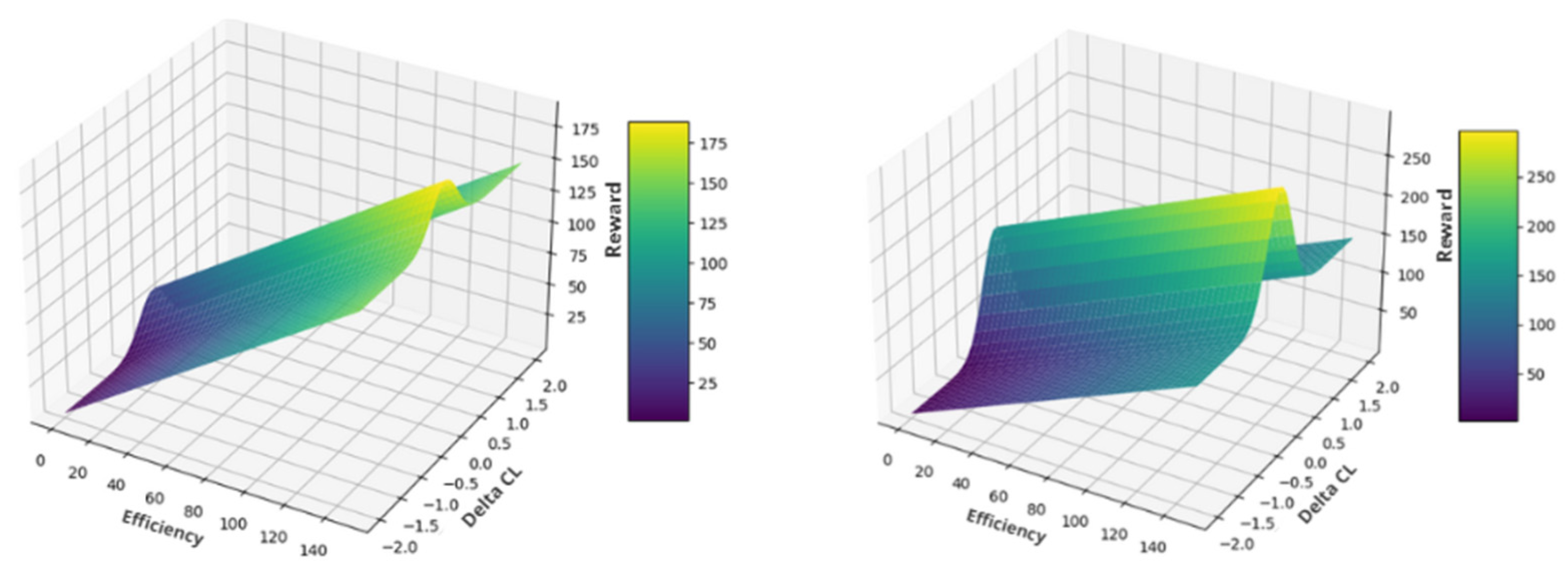
where $\mathsf{\alpha }$ is a parameter that defines the slope of $\mathrm{E}\left(\mathrm{s}\right)$, and $\mathsf{\beta }$ and $\mathsf{\gamma }$ are two parameters that characterise the Gaussian function, modifying the height and width of the bell curve, respectively. Some examples can be seen in Figure 8. This function is a combination of the previously mentioned linear function with an additional term that rewards the proximity of $\mathrm{C}\mathrm{L}\left(\mathrm{s}\right)$ to $\mathrm{C}{\mathrm{L}}_{\mathrm{o}\mathrm{b}\mathrm{j}\mathrm{e}\mathrm{c}\mathrm{t}\mathrm{i}\mathrm{v}\mathrm{e}}$. Using $\Delta \mathrm{C}\mathrm{L}\left(\mathrm{s}\right)$ instead of $\mathrm{C}\mathrm{L}\left(\mathrm{s}\right)$ directly normalises the function for any target value, allowing the agent to learn to minimise that value for any case without changing the rewards between different $\mathrm{C}{\mathrm{L}}_{\mathrm{o}\mathrm{b}\mathrm{j}\mathrm{e}\mathrm{c}\mathrm{t}\mathrm{i}\mathrm{v}\mathrm{e}}$ values, thus stabilising the learning process. It is crucial that the agent receives $\mathrm{C}{\mathrm{L}}_{\mathrm{o}\mathrm{b}\mathrm{j}\mathrm{e}\mathrm{c}\mathrm{t}\mathrm{i}\mathrm{v}\mathrm{e}}$ as input, as it allows the agent to recognise the case with which it is dealing.

The profiles obtained do not always seem to meet the CL target correctly. As shown in

Table 4. Comparison of CL target with the CL obtained using the reward function 9. The parameters of the equation are α = 1, β = 80 and γ = 15. The results of the highest rewards are shown for each case.

CL Target	0.30	CL Target	0.40	CL Target	0.60
Efficiency	77.87	Efficiency	82.74	Efficiency	78.60
CL	0.74	CL	0.81	CL	0.69
CL Error	0.44	CL Error	0.41	CL Error	0.09

, this has been particularly observed in low-lift profiles, as they tend to have low efficiency simply due to having a reduced CL. Therefore, the agent achieves better results by generating higher-lift profiles, which are much more efficient but with a CL significantly higher than desired, rendering them unusable. Therefore, a new equation must be sought to ensure that the CL target is met.

Thus, the following formula is defined:

$$\mathrm{r}(\mathrm{s})=\mathsf{\alpha }\mathrm{E}(\mathrm{s}){\mathrm{e}}^{-\mathsf{\gamma }{\left(\Delta \mathrm{C}\mathrm{L}\left(\mathrm{s}\right)\right)}^2}$$

(10)

where, like the previous case, $\mathsf{\alpha }$ is a parameter that adjusts the slope of the function, and $\mathsf{\gamma }$ is a parameter that determines the width of the Gaussian bell curve.

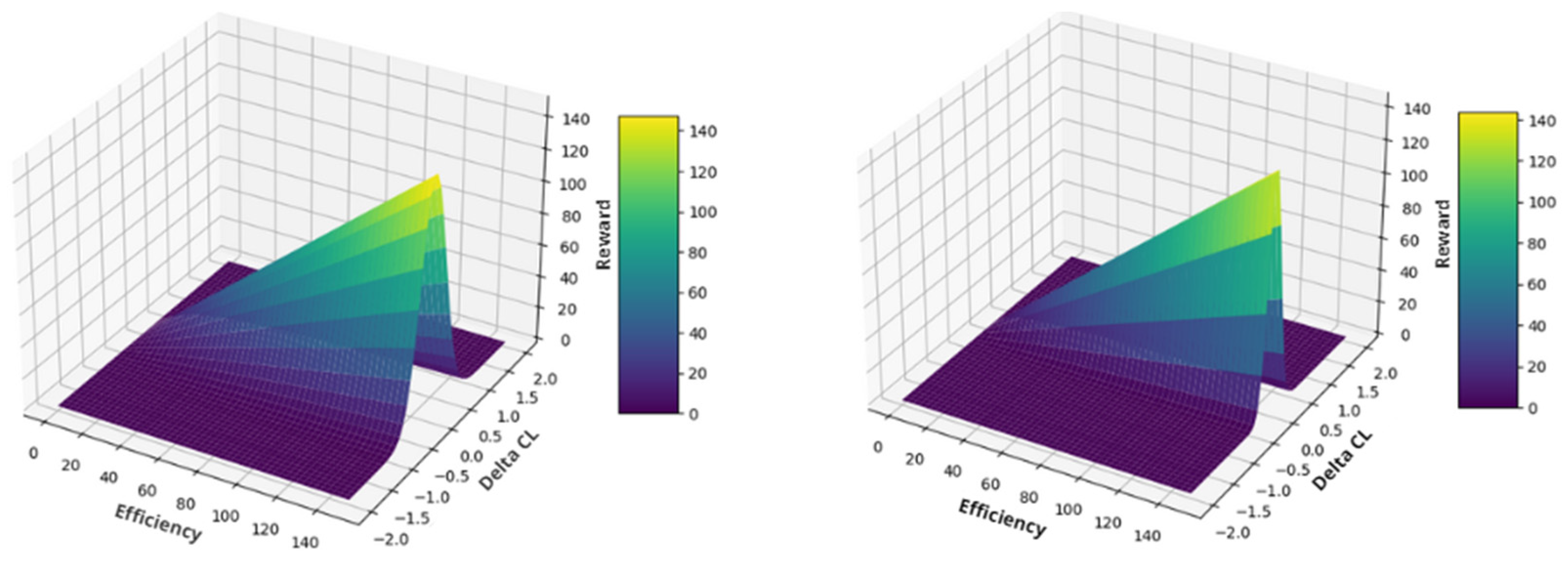
This function shares similarities with the previous one but removes the linear component. As seen in Figure 9, it is a Gaussian bell curve that increases in height as efficiency grows. This ensures that rewards are only obtained when CL is close to CL target, avoiding the issue.

In this case, the parameter $\mathsf{\gamma }$ plays a crucial role as it defines how strict the reward function is in relation to $\Delta C_L$. A lower value increases the width of the bell curve, allowing for profiles with higher efficiency but a lift coefficient different from the target. Conversely, a higher value imposes stricter limits, forcing the model to meet the requirements but making it harder to obtain efficient profiles.

Table 5. Comparison of CL target with CL obtained using the reward function 10. The parameters of the equation are α = 1, $\mathsf{\gamma }$ = 20. The results of the highest rewards are shown for each case.

CL Target	0.30	CL Target	0.40	CL Target	0.60
Efficiency	50.61	Efficiency	54.89	Efficiency	76.22
CL	0.40	CL	0.43	CL	0.69
CL Error	0.10	CL Error	0.03	CL Error	0.09

shows greater compliance with CL target, at the cost of a noticeable loss of efficiency due to the phenomenon.

In summary, there are numerous options when establishing the reward function. Equation (8) is a candidate for providing acceptable results for the target case, while if the objective is to focus on CL, Equation (10) appears to show the best results.

It is important to note that a wider Gaussian bell leads to lower precision with respect to the CL target, but the smoother shape of the reward function facilitates convergence. Conversely, a narrower Gaussian increases accuracy but makes training slower and more difficult due to the sharper reward landscape.

On the other hand, it is necessary to establish a significant penalty if the generated profile shows geometric anomalies, such as surface intersections. The agent may perform actions that result in these geometries, and just as a variable reward has been established based on the parameters mentioned earlier, a reward of −100 will be given if the profile is invalid. This establishes a clear distinction and will help the agent learn not to perform such actions. In the same process as verifying geometric anomalies, the constraint boxes are also checked.

Finally, an additional limitation has been introduced during profile verification, consisting of setting minimum thicknesses for the leading and trailing edges. This is due to initial training observations where the agent tended to create “spikes,” as shown in Figure 10. A possible explanation is the creation of an artificial angle of attack, producing a specific geometry that might go unnoticed by NeuralFoil’s neural network and fail to account for the aerodynamic effects this would cause. By establishing these minimum thicknesses, the problem has been resolved.

2.4. Training Configuration

2.4.1. Computational Resources

Table 6. Specifications of the computer used for the development of DRLFoil.

Element	Specification
CPU	Intel Core i7-14700K
GPU	NVIDIA GeForce RTX 4060 Ti 16 GB
RAM	32 GB (2×16 GB) DDR5 6000 MHz CL36
Storage	2 TB SSD M.2 Gen4
Operative System	Windows 11 Pro
CUDA	12.1
Python	3.10.11
PyTorch	2.3.0

shows the main components used for both the training and inferences of DRLFoil, as well as the versions of the main tools, with all results presented in this research being obtained using the same setup.

During training, n environments are used per step, and to achieve this, observations, actions, and rewards become vectors of dimension n. There are two different implementations. On one hand, DummyVecEnv allows environments to be vectorised in a single process, processing them in series. This simplifies debugging and requires fewer resources, as true parallelism does not exist. On the other hand, SubprocVecEnv uses multiple processes to run copies of the environment in parallel. This improves performance but consumes more resources and can be more complex. For the training conducted with DRLFoil, SubprocVecEnv is used to maximise the use of computational resources and accelerate training time.

2.4.2. Hyperparameter Optimisation

To achieve the best possible result during training, all hyperparameters must be adjusted using optimisation techniques [19]. RL Baselines3 Zoo [20] is a training framework that uses Stable Baselines 3, including numerous tools, one of which is hyperparameter optimisation. This specific task is performed using the Optuna framework [21], which conducts the optimisation automatically with several methods available.

The environment parameters used for the optimisation (whose names are described in

Table 7. Description of the parameters of the environment.

Parameter	Description
max_steps	Number of steps per episode
n_params	Number of weights per skin
scale_actions	Maximum variation of weights per step
airfoil_seed	Initial profile seed
cl_reward	Enable or disable the CL target
efficiency_param	Slope of reward growth
cl_wide	Width of the Gaussian bell curve
delta_reward	Difference between the current and previous step rewards. When enabled, the agent receives the relative change in performance instead of the absolute reward.
n_boxes	Number of constraint boxes

) can be seen in

Table 8. Environment parameters used in hyperparameter optimisation.

Parameter	Values
max_steps	10
n_params	10
scale_actions	0.15
airfoil_seed	Upper surface: [0.1, …, 0.1] Lower surface: [0.1, …, 0.1] Leading edge: [0.0]
cl_reward	True
efficiency_param	1
cl_wide	20
delta_reward	False
n_boxes	1

.

The method used is the Tree-structured Parzen Estimator, a popular variant of Bayesian optimisation methods for hyperparameter tuning [22]. A total of thirty-five different trials are conducted, each using a different combination of hyperparameters, with 600,000 steps per trial. This results in a total of 21,000,000 steps—a high number. To reduce the optimisation time, a technique called pruning is used, which consists of early stopping for inefficient trials. The median method is used, which stops a trial if its intermediate performance is worse than the median of all trials at the same stage.

After the optimisation, the results of all trials were synthesised in

Table 9. Comparison of the rewards obtained after 600,000 steps. The six best resulting models are shown, as well as the unoptimized model used so far.

Model	Mean Reward
1	311
2	31
3	20
4	5
5	1
6	−3
Not Optimised	−100

, where the top six are shown. Since the number of steps performed in each trial is limited, it is crucial to conduct a full trial with the best candidates to analyse their real performance in detail.

Using the environment parameters from Table 8, five different training sessions were conducted: four of them correspond to the best models obtained from the optimisation, while the last one uses the hyperparameters from Table 3, with the modifications mentioned in subsequent paragraphs regarding learning rate and network size. The training sessions last for two million steps, and the history of the average rewards obtained can be seen in Figure 11. As expected, the first model presents the best results, followed by the second. The fourth model, despite showing satisfactory results during optimisation, stagnates prematurely.

In summary, the hyperparameters selected for the final development phase are those shown in

Table 10. Hyperparameters selected as a basis after optimisation, making use of one constraint box.

Hyperparameter	Value	Hyperparameter	Value
learning_rate	0.000268	clip_range_vf	None
n_steps	32	ent_coef	0.001
batch_size	512	vf_coef	0.754843
n_epochs	20	max_grad_norm	5
gamma	0.995	target_kl	None
gae_lambda	0.98	net_arch	64, 64
clip_range	0.3	Activation_fn	Tanh

. It has been demonstrated that slight variations in these parameters are useful depending on the scenario presented (especially noteworthy is the change in network size, which will be applied in the final models in the section).

3. Results and Discussion

3.1. Configuration

The hyperparameters used, except for the network architecture, which will vary for each model, can be seen in Table 8. The environment employed is common across all models, and the defining parameters are shown in

Table 11. Environment parameters used by the final models.

Parameter	Value
max_steps	10
n_params	8
scale_actions	0.3
airfoil_seed	Upper surface: [0.3, …, 0.3] Lower surface: [0.3, …, 0.3] Leading edge: [0.0]
efficiency_param	1
cl_wide	20

. These were determined after conducting a sensitivity analysis of each characteristic, yielding several conclusions. Firstly, it was observed that using a larger number of weights per curve of the profile resulted in anomalous geometries, due to overfitting by the agent, which produces unreliable results in real-world applications. Secondly, the scaling of actions was reduced, meaning that each action performed by the agent is limited in its modifications, which stabilises the training by preventing abrupt changes. Finally, the initial profile seed was set to fixed parameters. This ensures that each time the environment is reset, the initial profile remains the same, leaving exploration to the randomness of the agent’s actions. The rest of the parameters correspond to other adjustments previously discussed.

For model training, minimum and maximum values were set for both the target lift coefficient and the Reynolds number. Defining this range is crucial not only to prevent the user from imposing unrealistic conditions but also to facilitate the agent’s training by reducing the number of cases to consider. The limits are listed in

Table 12. Operating ranges of target lift coefficient and Reynolds number.

Parameter	Minimum	Maximum
CL target	0.1	1.6
Reynolds	100,000	50,000,000

.

The CL target has been restricted to positive values only, excluding values below 0.1, as the agent would not be able to optimise the profile due to the resulting negligible efficiency.

The minimum Reynolds number is set at 100,000, as it was found that NeuralFoil produces erratic results when the number is below this threshold. On the other hand, the maximum value of fifty million covers a wide range of operations for drones and even small aircraft. For example, an aircraft with a 2 m chord and a speed of 100 m/s has a Reynolds number of approximately 14,000,000. In contrast, a drone with a 0.3 m chord and a speed of 23 m/s has a Reynolds number close to 500,000.

3.2. Model Without Restriction Box

The current model is characterised by not using any form of dimensional constraint, making it the simplest case. Therefore, the only constraints that can be imposed by the user are the CL target and the desired Reynolds number, which simplifies its training due to the reduction in the number of observations. As a result, the network size, both for the actor and the critic, consists of two layers with thirty-two neurons each. The number of hidden layers (two) and neurons per layer was selected empirically to balance model capacity and training stability. Larger networks were tested during preliminary trials and led to overfitting or slower convergence, while smaller ones were insufficient to capture the nonlinear aerodynamic dependencies.

The training results can be seen in Figure 12, which shows the average reward obtained as a function of the step. Additionally, an evaluation of the model’s performance is conducted, and the results are shown in

Table 13. Rewards obtained in the evaluation of the agent in thirty random scenarios.

Evaluation	Mean	Standard Deviation
General	1036.06	382.31
CL target = 0.3	586.77	101.37
CL target = 0.6	991.91	233.73
CL target = 0.9	1352.89	231.55
CL target = 1.2	1395.8	140.71
CL target = 1.5	1238.75	340.43

, based on thirty random evaluations where the accumulated reward was recorded for each episode. The table first shows a general evaluation where both the CL target and the Reynolds number are random. Subsequently, different evaluations are conducted where the CL target is fixed, allowing an analysis of how each range of CL affects the reward. Since the reward is related to efficiency, it logically increases with an increase in the lift coefficient. It is also interesting to observe the standard deviation, which shows the variation in rewards obtained in each episode, primarily caused by fluctuations in the Reynolds number.

Table 14. Results obtained for a fixed Reynolds value of 1,000,000.

CL Target	CL Obtained	Difference	CD Obtained	Efficiency
0.1	0.225	0.125	0.007	33.195
0.3	0.36	0.06	0.008	43.704
0.5	0.531	0.031	0.008	68.981
0.7	0.746	0.046	0.01	77.644
0.9	0.959	0.059	0.011	90.067
1.1	1.113	0.013	0.014	80.394
1.3	1.225	−0.075	0.014	87.353
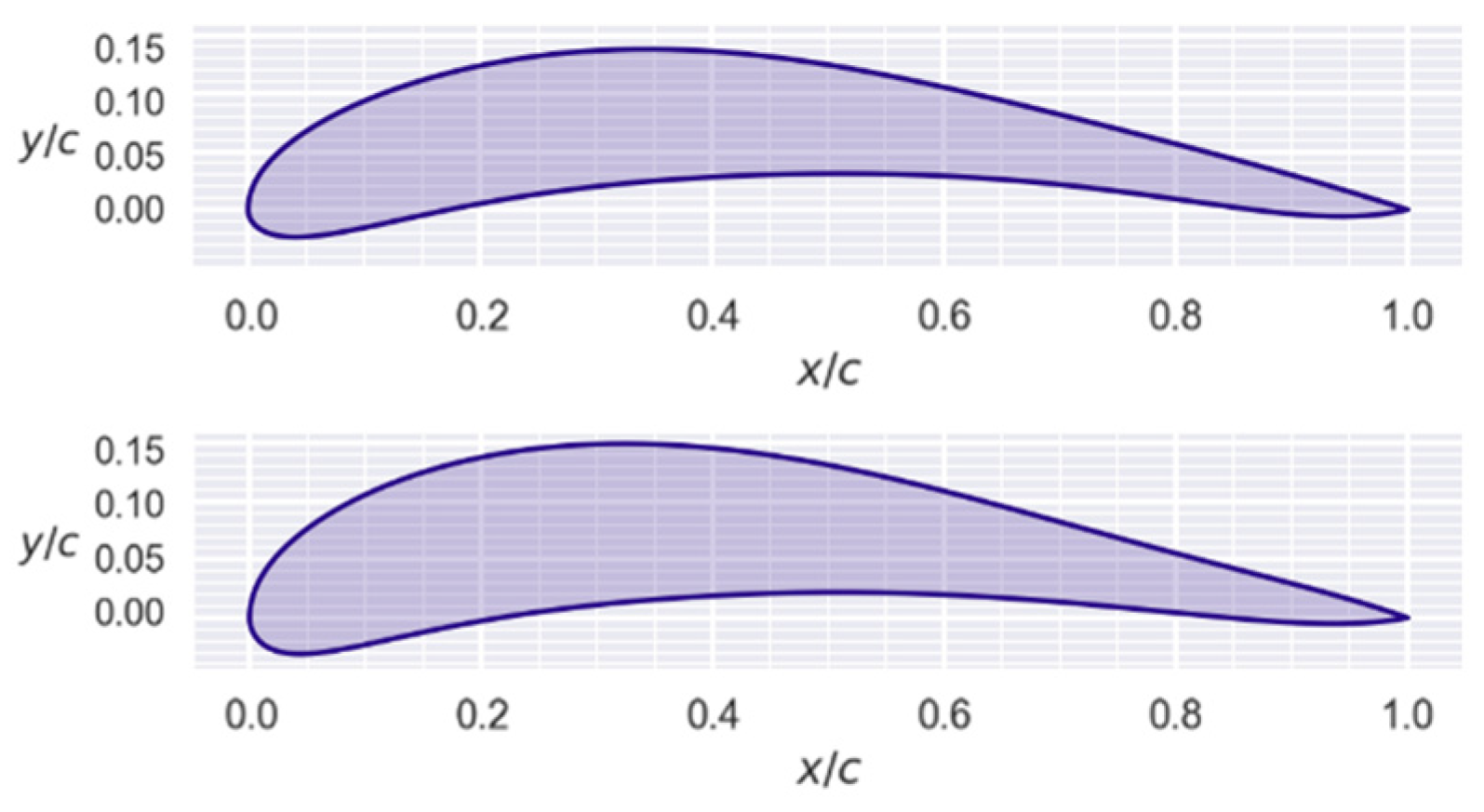
1.5	1.313	−0.187	0.017	77.894

presents different optimisation processes, each consisting of ten steps, selecting the profile with the best results. As can be observed, the accuracy obtained in CL is high, keeping in mind that this could be improved by modifying the width of the Gaussian bell curve in the reward function (see Figure 9). Additionally, the geometries shown in Figure 13 display considerable similarities to conventionally used profiles, demonstrating the model’s ability to converge to realistic policies. The average time for an optimisation process, using a total of ten steps, is 0.108 s.

Furthermore, in

Table 15. Results obtained for a fixed value of CL target of 0.6.

Reynolds	CL Obtained	Difference	CD Obtained	Efficiency
100,000	0.583	−0.017	0.032	17.958
300,000	0.623	0.023	0.014	45.441
500,000	0.622	0.022	0.011	55.501
1,000,000	0.627	0.027	0.08	74.043
3,000,000	0.611	0.011	0.07	90.149
5,000,000	0.609	0.009	0.06	100.311
10,000,000	0.616	0.016	0.05	113.093
40,000,000	0.607	0.007	0.05	128.499

, a similar comparison is made, this time fixing the target lift coefficient at 0.6 and allowing an analysis of how the agent responds to variations in the Reynolds number. As expected, efficiency increases proportionally, remaining low when the Reynolds number is low and increasing significantly at higher Reynolds numbers. In Figure 14, the slight changes in profiles for different Reynolds values can be observed, showing that the agent is able to understand the influence of this parameter on the optimisation process.

3.3. Model with a Restriction Box

After confirming how an agent can generate optimal profiles without dimensional constraints, this section analyses the model’s ability to interpret a constraint box. As explained earlier, this involves adding four additional parameters to the observations, corresponding to the dimensions of the box and its two position coordinates. Naturally, this increases the model’s inherent difficulty, which can be observed in the difference in network size between this model and the previous one. In this case, the architecture still consists of two layers, but each layer uses 128 neurons.

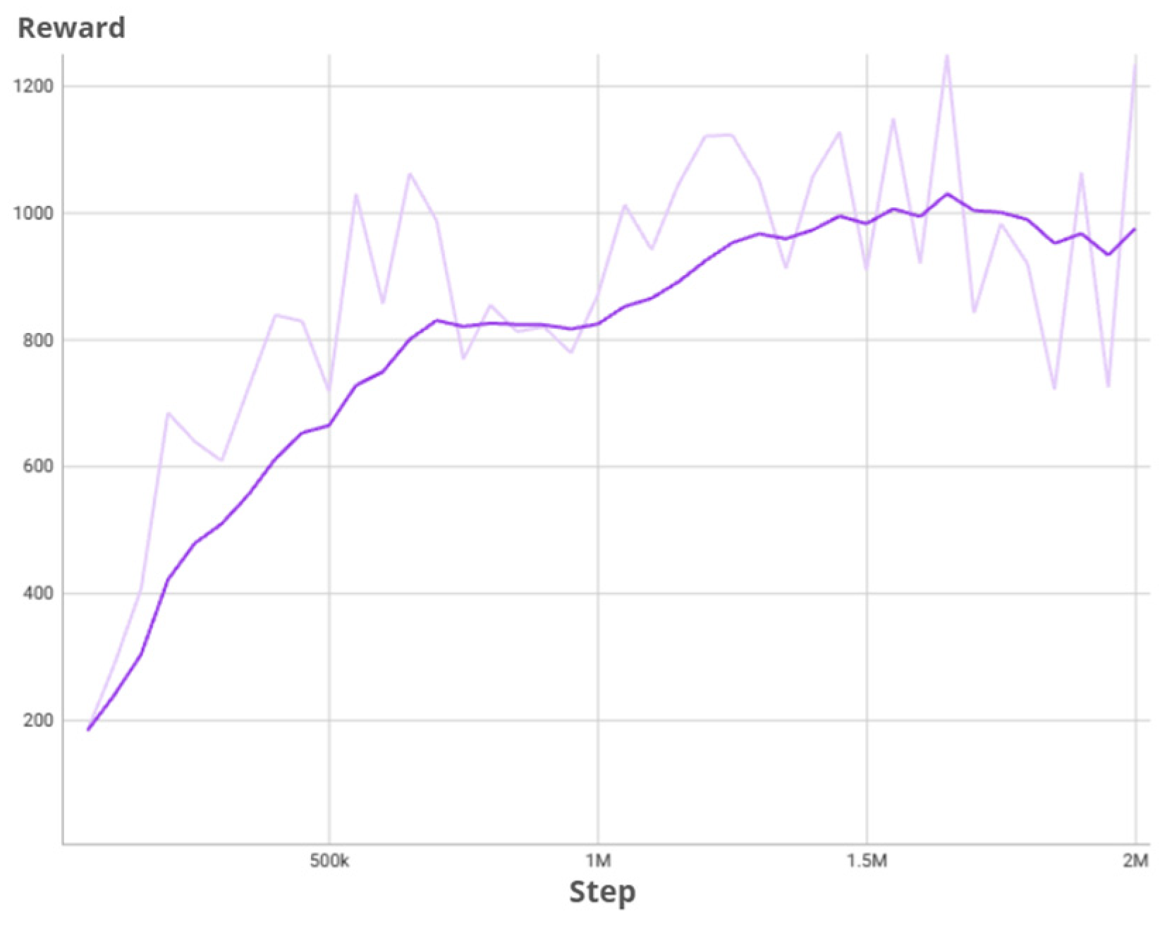
In Figure 15, the reward graph as a function of steps can be seen, using one million more steps than the previous agent due to its slower convergence.

Table 16. Rewards earned in the agent’s evaluation with a box in thirty random scenarios.

Evaluation	Mean	Standard Deviation
General	712.25	262.26
CL target = 0.3	483.72	78.62
CL target = 0.6	782.38	158.52
CL target = 0.9	925.88	97.28
CL target = 1.2	842.97	293.73
CL target = 1.5	646.77	11.12

shows the agent’s evaluation under different circumstances, where a key difference from Table 13 can be noted: once the CL exceeds one, the agent begins to struggle to generate optimal profiles. This can be interpreted because of the reward diminishing when the CL target reaches 1.2, unlike the previous model, where this value corresponds to the maximum reward.

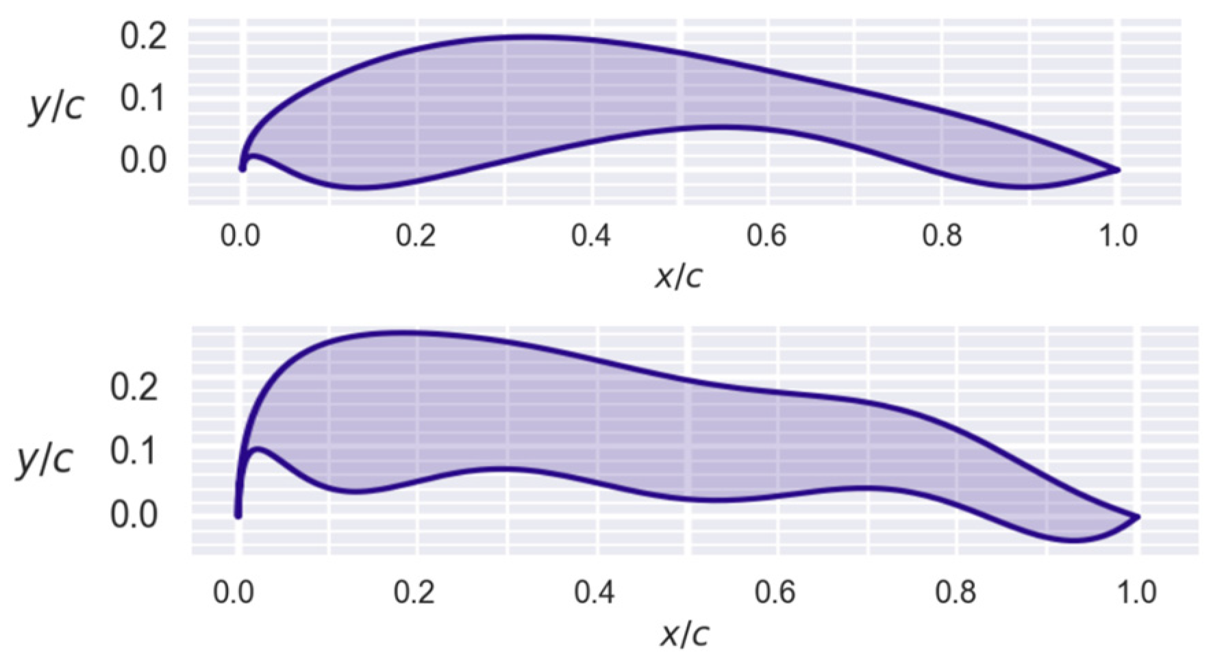
Some examples of optimised profiles can be seen in Figure 16, where, under the same CL target condition, the agent attempts to meet the imposed dimensional constraints.

It is clearly evident how all profiles share common characteristics, something that is not as drastic in Figure 17. Given the high value of the CL target, the agent requires more complex geometries to satisfy the imposed requirements.

Finally,

Table 17. Results obtained for a fixed constraint box and Reynolds value of 10,000,000.

CL Target	CL Obtained	Difference	CD Obtained	Efficiency
0.1	-	-	-	-
0.3	0.347	0.047	0.006	57.921
0.5	0.511	0.011	0.006	85.713
0.7	0.709	0.009	0.008	91.408
0.9	0.901	0.001	0.009	101.138
1.1	1.082	−0.018	0.010	106.099
1.3	1.223	−0.077	0.013	94.055
1.5	1.324	−0.176	0.017	80.092

provides a performance study of the model under the same Reynolds number and the same constraint box, which can be observed in Figure 18. This example was chosen because it represents several common situations encountered when optimising with this model. As can be seen, the extreme cases of the CL target have been the most challenging. When the value was 0.1, the agent was unable to provide a valid result, while at 1.5, the CL obtained showed the greatest deviation. However, excluding these two cases, the results demonstrate a strong ability to adapt to the constraints while maintaining high efficiency, even at high lift coefficients where the constraint box significantly limits the possibility of curving the profile.

3.4. Model with Two Restriction Boxes

Finally, the agent capable of interpreting two-dimensional constraint boxes is presented, which adds eight additional parameters to the observation. This is the most complex model trained in this work, as it was considered unnecessary to include a model capable of managing a greater number of boxes, given the added difficulty this task poses for the neural network. The architecture is made up of two layers with 256 neurons each, making it the largest model of the three studied.

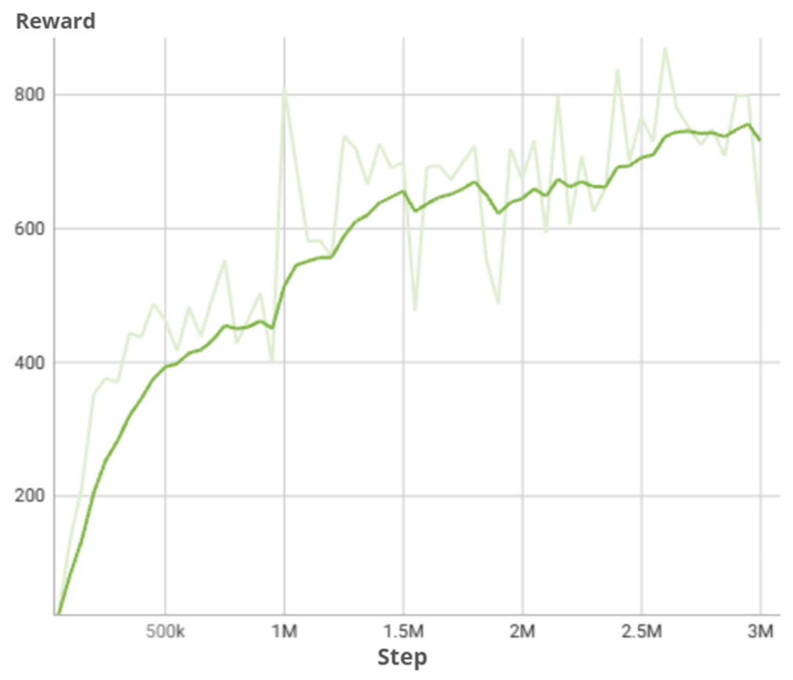
Figure 19 shows the training graph, reaching up to five million steps and demonstrating a slightly slower reward convergence speed compared to the case with one constraint box.

Table 18. Rewards earned in the two-box agent evaluation in thirty random scenarios.

Evaluation	Mean	Standard Deviation
General	611.71	160.58
CL target = 0.3	402.82	147.22
CL target = 0.6	589.92	216.12
CL target = 0.9	669.64	166.91
CL target = 1.2	639.83	179.71
CL target = 1.5	459.33	118.32

presents the evaluation results, using the same procedure as in the one-box model to ensure equal conditions. In this case, although the rewards increase with the CL target, similar to the previous models, the differences are not as pronounced as they were before. This suggests a difficulty for the model in achieving high efficiencies.

Some optimisation cases are shown in Figure 20, where the model’s ability to adapt the geometry of the profiles to the constraints imposed by the boxes can be observed. This opens possibilities for optimisation applied to real-world scenarios, such as the presence of passing structures, contained loads, or even the use of constraint boxes with the sole purpose of obtaining different aerodynamic profile concepts.

Thus, we can conclude that the model demonstrates a high capacity to adapt to complex environments, as well as the ability to meet demanding requirements, such as a high CL target, in a satisfactory manner by using complex and unconventional geometries.

4. Conclusions and Future Works

The research successfully demonstrates the application of Deep Reinforcement Learning (DRL) to aerodynamic profile optimisation for aerodynamic efficiency while explicitly learning to satisfy geometric constraints. Through the integration of Proximal Policy Optimisation (PPO), the research has effectively shown the potential for real-time optimisation of constrained geometries, in environments characterised by strict spatial and aerodynamic requirements. The results indicate that the methodology achieves rapid convergence and high precision across a wide range of Reynolds numbers and CL target values, validating the feasibility of applying DRL to geometrically constrained aerodynamic scenarios.

As a result of the methodology, a tool has been developed that allows users to dynamically define several optimisation parameters and introduce spatial restrictions such as internal bounding boxes. This versatility enables adaptation to a variety of scenarios, including morphing wings and configurations with internal payload or structural limitations. The computational efficiency achieved by the pre-trained neural networks ensures that the geometries of aerodynamic profiles can be optimised in milliseconds, a key factor for real-time applications. This achievement bridges the gap between traditional computational fluid dynamics (CFD) methods and real-time requirements, offering a more efficient alternative without sacrificing accuracy.

The robustness of the PPO algorithm, particularly its ability to adapt to different aerodynamic and geometric conditions, has been evident throughout the study. For example, the agent’s response to variations in Reynolds numbers illustrates its ability to effectively understand and leverage environmental parameters. This behaviour highlights the importance of selecting appropriate reinforcement learning algorithms when addressing real-world optimisation problems with complex geometric feasibility domains. Additionally, the decision to normalise the action and observation spaces contributed to the stability and efficiency of the learning process, preventing overfitting, and ensuring smooth convergence.

The research opens several avenues for future work. One potential direction is to expand the current framework to optimise multiple and potentially conflicting objectives simultaneously, for instance maximising aerodynamic efficiency and structural integrity while maintaining target lift distribution and manufacturability constraints. This approach would require the development of more sophisticated reward structures that account for trade-offs between aerodynamic, structural, and geometric performance metrics. Furthermore, exploring the integration of Transfer Learning within the DRLFoil environment could improve the initial training phase, allowing agents to learn from pre-existing data before adapting to specific aerodynamic or geometric conditions. Another promising line of research involves the use of computer vision or generative models to automatically infer geometric constraints from simplified or visual design inputs, allowing the agent to adapt the optimisation space to predefined structural or integration requirements. Finally, real-time implementation on embedded systems could enable onboard morphing or adaptive design, with UAVs autonomously adjusting their shape in response to changing flight conditions, illustrating the broader potential of this framework for adaptive and constraint-aware aerodynamics.

References

1. Boom Supersonic. Available online: https://boomsupersonic.com/ (accessed on 21 May 2025).
2. Lampton, A.; Niksch, A.; Valasek, J. Reinforcement Learning of a Morphing Airfoil-Policy and Discrete Learning Analysis. J. Aerosp. Comput. Inf. Commun. 2010, 7, 241–260. [Google Scholar] [CrossRef]
3. Chen, H.; Gao, C.; Wu, J.; Ren, K.; Zhang, W. Study on Optimization Design of Airfoil Transonic Buffet with Reinforcement Learning Method. Aerospace 2023, 10, 486. [Google Scholar] [CrossRef]
4. Jiang, W.; Zheng, C.; Hou, D.; Wu, K.; Wang, Y. Autonomous Shape Decision Making of Morphing Aircraft with Improved Reinforcement Learning. Aerospace 2024, 11, 74. [Google Scholar] [CrossRef]
5. Yan, X.; Zhu, J.; Kuang, M.; Wang, X. Aerodynamic shape optimization using a novel optimizer based on machine learning techniques. Aerosp. Sci. Technol. 2019, 86, 826–835. [Google Scholar] [CrossRef]
6. Dussauge, T.P.; Sung, W.J.; Fischer, O.J.; Mavris, D.N. A reinforcement learning approach to airfoil shape optimization. Sci. Rep. 2023, 13, 9753. [Google Scholar] [CrossRef] [PubMed]
7. Hui, X.; Wang, H.; Li, W.; Bai, J.; Qin, F.; He, G. Multi-object aerodynamic design optimization using deep reinforcement learning. AIP Adv. 2021, 11, 085311. [Google Scholar] [CrossRef]
8. Viquerat, J.; Rabault, J.; Kuhnle, A.; Ghraieb, H.; Larcher, A.; Hachem, E. Direct shape optimization through deep reinforcement learning. J. Comput. Phys. 2021, 428, 110080. [Google Scholar] [CrossRef]
9. Li, R.; Zhang, Y.; Chen, H. Learning the aerodynamic design of supercritical airfoils through deep reinforcement learning. AIAAJ 2021, 59, 3988–4001. [Google Scholar] [CrossRef]
10. de Bruin, T.; Kober, J.; Tuyls, K.; Babuška, R. Fine-tuning Deep RL with Gradient-Free Optimization. IFAC-PapersOnLine 2020, 53, 8049–8056. [Google Scholar] [CrossRef]
11. Shakya, A.K.; Pillai, G.; Chakrabarty, S. Reinforcement learning algorithms: A brief survey. Expert Syst. Appl. 2023, 231, 120495. [Google Scholar] [CrossRef]
12. Raffin, A.; Gleave, A.; Kanervisto, A.; Ernestus, M.A.D.N. Stable-Baselines3 2021. Available online: https://github.com/DLR-RM/stable-baselines3 (accessed on 17 June 2025).
13. Raffin, A.; Gleave, A.; Kanervisto, A.; Ernestus, M.A.D.N. Stable-Baselines3: Reliable Reinforcement Learning Implementations. J. Mach. Learn. Res. 2021, 22, 268. [Google Scholar]
14. Towers, M.; Kwiatkowski, A.; Terry, J.; Balis, J.U.; de Cola, G.; Deleu, T.; Goulão, M.; Kallinteris, A.; Krimmel, M.; KG, A.; et al. Gymnasium: A Standard interface for reinforcement learning environments. arXiv 2024, arXiv:2407.17032. [Google Scholar] [CrossRef]
15. Sharpe, P. NeuralFoil 2023. Available online: https://github.com/peterdsharpe/NeuralFoil (accessed on 24 June 2025).
16. Sharpe, P.; Hansman, R.J. NeuralFoil: An Airfoil Aerodynamics Analysis Tool Using Physics-Informed Machine Learning. arXiv 2025, arXiv:2503.16323. [Google Scholar]
17. Sharpe, P.D. AeroSandbox Massachusetts Institute of Technology. 2021. Available online: https://peterdsharpe.github.io/AeroSandbox/ (accessed on 3 May 2025).
18. Achleitner, J.; Rohde-Brandenburger, K.; Hornung, M. Airfoil optimization with CST-parameterization for (un-)conventional demands. In Proceedings of the XXXIV OSTIV Congress, Hosin, Czech Republic, 28 July–4 August 2018. [Google Scholar]
19. Bischl, B.; Binder, M.; Lang, M.; Pielok, T.; Richter, J.; Coors, S.; Thomas, J.; Ullmann, T.; Becker, M.; Boulesteix, A.; et al. Hyperparameter Optimization: Foundations, Algorithms, Best Practices and Open Challenges. WIREs Data Min. Knowl. Discov. 2021, 13, e1484. [Google Scholar] [CrossRef]
20. Raffin, A. RL Baselines3 Zoo. 2020. Available online: https://github.com/DLR-RM/rl-baselines3-zoo (accessed on 17 June 2025).
21. Networks, I.P. Optuna. Available online: https://optuna.org/ (accessed on 7 July 2025).
22. Watanabe, S. Tree-Structured Parzen Estimator: Understanding Its Algorithm Components and Their Roles for Better Empirical Performance. arXiv 2023, arXiv:2304.11127. [Google Scholar] [CrossRef]
Figure 1. Structure of a Reinforcement Learning algorithm [6].
Aerospace 12 00971 g001
Figure 2. Scheme of deep reinforcement learning agents [11].
Aerospace 12 00971 g002
Figure 3. Comparison of analyses obtained with NeuralFoil and XFOIL models [15].
Aerospace 12 00971 g003
Figure 4. Flow chart of the optimisation process.
Aerospace 12 00971 g004
Figure 5. Block diagram of the inference process.
Aerospace 12 00971 g005
Figure 6. Examples of restriction boxes (blue and red rectangles). At the top are valid profiles, while at the bottom are invalid profiles.
Aerospace 12 00971 g006
Figure 7. Diagram of the DRLFoil PPO network.
Aerospace 12 00971 g007
Figure 8. Representation of the linear-Gaussian function of the reward, with value. (Left), β = 40 and γ = 5 ; (right), β = 150 and γ = 5 .
Aerospace 12 00971 g008
Figure 9. Representation of the Gaussian function of the reward, with value α = 1 . (Left), γ = 5 ; (right), γ = 20 .
Aerospace 12 00971 g009
Figure 10. Generation of peaks in the profiles.
Aerospace 12 00971 g010
Figure 11. Plot of average rewards as a function of pace obtained in each model.
Aerospace 12 00971 g011
Figure 12. Graph of average rewards for the model without boxes.
Aerospace 12 00971 g012
Figure 13. Profiles obtained for different CL targets: (above left), 0.4; (above right), 0.7; (bottom left), 1; (bottom right), 1.3.
Aerospace 12 00971 g013
Figure 14. Comparison of two profiles at different Reynolds: (top), 100,000; (bottom), forty million.
Aerospace 12 00971 g014
Figure 15. Graph of average rewards for the one-box model.
Aerospace 12 00971 g015
Figure 16. Profiles generated with a CL target of 0.4 and Reynolds number of 10,000,000.
Aerospace 12 00971 g016
Figure 17. Profiles generated with a CL target of 0.9 and Reynolds number 10,000,000.
Aerospace 12 00971 g017
Figure 18. Comparison of two profiles with the same constraint box and Reynolds number 10,000,000. (left), CL target of 0.3; (right), 1.3.
Aerospace 12 00971 g018
Figure 19. Average reward graph of the two-box model.
Aerospace 12 00971 g019
Figure 20. Airfoils generated with a CL target of 0.4 and Reynolds number of 10,000,000.
Aerospace 12 00971 g020