Abstract
To enhance the objectivity and precision of quality evaluation in flight training, this study proposes an assessment method for the landing flare phase based on time-series flight parameter data from Secure Digital (SD) card. By analyzing landing flare data from flight instructors and trainees, a standard sequence model was established, and the Dynamic Time Warping (DTW) algorithm was employed to calculate the similarity between individual trainee sequences and the standard sequence. Using K-means clustering, the landing flare quality was categorized into four distinct levels: Excellent (22.5%), Good (25.5%), Qualified (23.5%), and Improvement Needed (28.5%). The results demonstrated significant consistency with instructor evaluations (Spearman correlation coefficient 0.71). Furthermore, through the identification of weak parameters, specific technical deficiencies in areas such as airspeed control and pitch attitude maintenance could be accurately pinpointed. This approach not only effectively validates and supplements instructor assessments but also provides data-driven support for developing personalized training programs, thereby improving the quality and efficiency of flight training.
1. Introduction
According to Boeing’s 2025 Pilot and Technician Outlook (PTO) [1], the global civil aviation industry will require nearly 2.4 million new aviation professionals by 2044 to support long-term growth in air travel, including 660,000 new pilots. This has led to a growing demand for high-quality pilots, making pilot training a critical task. The period of flight training is a key phase in the development of their flight skills, as the training received during this time directly affects the stability and safety of their subsequent flight operations. Flight quality assessment serves as the standard for measuring the flight quality of trainees, but traditional methods primarily rely on subjective judgments by instructors, leading to issues related to consistency and efficiency.
Researchers both domestically and internationally have conducted studies in the area of pilot flight quality assessment, including the development of evaluation frameworks for flight trainees, as well as the use of methods like the Analytic Hierarchy Process and Fuzzy Comprehensive Evaluation to assess flight quality [2,3,4,5,6]. However, these methods often involve significant subjectivity in determining the weight of evaluation indicators. In recent years, with the widespread use of airborne data recording devices, data-driven methods for flight quality assessment have become a research hotspot. These methods include building flight quality assessment models using flight parameter data and pilot behavior data [7,8,9,10,11,12], as well as integrating machine learning algorithms for evaluating pilot performance [13,14,15,16,17]. While these methods offer new technical approaches and perspectives in flight data analysis and training assessment, they have notable limitations in terms of applicability and interpretability in practical operations, and their efficiency in personalized pilot assessments still needs improvement. Therefore, there is a need to develop a flight quality assessment method based on objective quantitative data, integrated with instructors’ subjective experiential judgments, to form more comprehensive evaluation conclusions.
Flight data is essentially time-series data that contains dynamic information about various parameters changing over time during flight. The Transformer Encoder models global temporal dependencies directly through the self-attention mechanism and supports parallel computation. Compared to Autoregressive Integrated Moving Average (ARIMA), Long Short-Term Memory (LSTM), and Gated Recurrent Unit (GRU), it offers superior modeling capability and computational efficiency when handling long sequences and multivariate time series data. These advantages have been validated in the field of multivariate time series modeling and analysis [18,19]. Currently, there is a lack of research on time-series similarity analysis for flight data; however, when utilizing flight parameters for refined assessment of handling qualities, most existing studies rely on analyzing statistical characteristics of discrete parameter points (such as extreme values, means) or exceedance event counts. There remains a lack of quantitative evaluation methods capable of effectively capturing the differences in the overall dynamic patterns between complete landing maneuver time series data and standard procedures. Time-series similarity measurement methods [20,21,22] are effective data mining techniques, with common methods including Euclidean distance, DTW [23,24], and Singular Value Decomposition (SVD). Some scholars have already used the DTW method to conduct studies on motion extraction and trajectory prediction in the field of transportation [25,26]. By taking into account the covariance structure among multivariate variables, Mahalanobis distance effectively eliminates the influence of scale differences and captures the correlations between features. Compared to Euclidean distance, it is more suitable for multivariate DTW-based time series similarity measurement, and its advantages have been validated in previous studies [27,28]. By applying time-series similarity analysis, the similarity between each pilot’s flight data and standard flight data can be computed, offering an objective, quantitative assessment of flight quality and providing new insights for flight quality evaluation.
In terms of research phase delineation, existing studies predominantly focus on the complete approach or landing process, relying on static statistical feature analysis of flight parameters or traditional machine learning models [29]. However, the landing flare phase possesses unique analytical value: the aircraft operates in a critical state of low altitude and low speed, where any operational deviation may lead to severe consequences. Although brief, this phase intensively reflects pilots’ fine control skills and serves as a key indicator for distinguishing proficiency levels. Nevertheless, current research remains insufficient in conducting deep time-series analysis of this specific phase. This study precisely defines its analytical scope as the flare phase, aiming to achieve more refined assessment of handling qualities.
Regarding the selection of flight parameters, one approach quality evaluation study [30] primarily relied on three parameters: airspeed, pitch angle, and localizer deviation. Another study on landing safety prediction [31] employed three flight parameters for analysis, yet the model suffers from structural complexity, combinatorial redundancy, and poor interpretability. It is noteworthy that a study on wind shear operations [32] adopted five key parameters, demonstrating comprehensive consideration of flight parameters, but its focus was on extreme weather conditions. Similarly, a study covering the complete landing process [33] utilized an extensive parameter set, yet its analysis spanned multiple phases without in-depth examination of the transient flare process. Consequently, this study concentrates on the landing flare phase under normal conditions, systematically integrating complete time series of key parameters. Through continuous dynamic analysis, it achieves multidimensional and more targeted evaluation of handling qualities in this phase.
In summary, this paper leverages key parameters from the landing flare phase to propose a quality assessment method based on time-series similarity measurement. First, a Transformer encoder is used to model the flight instructor’s flight data in a temporal sequence, outputting a standard multidimensional landing time series as a template. Then, the DTW method is applied to measure the similarity between the flight trainee’s multidimensional landing time series and the template. Next, K-means clustering is used to cluster the similarity measurement values, and a comparative analysis was conducted between the evaluation results and instructor ratings. Finally, through the identification of weak parameters and visual curve analysis, the specific weak flight parameters of the trainee are identified, providing data support for the development of a personalized training plan for the trainee.
2. Phase Delineation, Data and Methods
2.1. Phase Delineation
According to Boeing’s Statistical Summary of Commercial Aviation Accidents 2024 [34], although the landing phase accounts for only 1% of total flight time, its fatality accident rate constitutes 37% of all transport aviation accidents. From a human–machine systems engineering perspective, pilots face dual pressures of high cognitive load and narrow decision-making windows during landing, requiring precise coordination of multiple parameters and parallel processing of multiple tasks within limited time.
The flare phase—transitioning from stabilized approach to touchdown—epitomizes the extremity of these challenges. During this critical period, pilots must execute a series of high-precision operations including trajectory transition, attitude coordination and energy management at low altitude, thereby making the quality of control operations directly determinant of landing safety and operational efficiency. Consequently, the flare phase represents not only the technical core of the landing sequence but also a crucial window for assessing pilots’ fine control capabilities and identifying potential technical deficiencies. This study precisely focuses on this phase due to its critical safety significance and unique technical challenges.
According to the International Civil Aviation Organization (ICAO) Accident/Incident Data Reporting (ADREP) taxonomy [35], this phase begins when the aircraft transitions from the final approach attitude to the landing attitude (flare initiation) and ends when the main landing gear touches the runway. We adopted the standard operating procedures (SOPs) for the DA40NG aircraft at a designated training airport as the benchmark. This benchmark describes the expected characteristics of an ideal landing flare: Initiation Altitude:The maneuver starts at approximately 140–150 ft above ground level. Target Airspeed: The baseline target approach speed is 80 knots upon entry, smoothly decreasing to touchdown speed during the process. Flight Path: The expected flare trajectory is a smooth, continuous reduction in descent rate, aimed at achieving a gentle touchdown. The ideal vertical flight path angle is approximately −3°, gradually leveling off toward the end of the flare. Operational Objective: The core control objective of the flare phase is to manage airspeed and descent rate through smooth back-pressure control on the control column, ultimately achieving a smooth main-wheel touchdown within the designated runway aiming zone.
The data window used for analysis in this study spans from the defined initiation point described above until main-wheel touchdown. Preliminary analysis of the dataset indicated that this phase typically lasts within 30 s under the specified aircraft type and airport conditions. Consequently, a fixed sequence length of T = 30 s was established as the standard. This setting ensures the analytical window fully captures the complete control sequence from flare initiation to touchdown in the studied operational environment, thereby guaranteeing operational integrity.
2.2. Data
The data were collected through an integrated avionics system developed and manufactured by Garmin. The Garmin G1000 integrated avionics system is equipped with numerous sensors that automatically store the acquired flight data on the system’s built-in onboard SD card, with a recording frequency of 1 Hz. The SD card contains a wealth of flight data. Using the Diamond DA40 as an example, the primary flight data includes indicated airspeed (IAS), altitude (AltMSL), vertical speed (VSpd), pitch angle (Pitch), and track angle (TRK), among others. All data processing in this study adhered to privacy protection protocols, ensuring the security of trainees’ personal information. The flight data used during the research underwent anonymization procedures and complies with scientific research ethics requirements.
During the landing process, establishing a stable landing condition essentially involves the precise control of landing parameters. The selection of evaluation parameters is a key aspect of flight assessment. Flight trainees refer to the training syllabus and subjects during their training, with corresponding standards for different flight stages. Therefore, flight parameters can intuitively reflect the trainees’ operational performance. The landing process involves controlling altitude and descent rate while maintaining an appropriate flight attitude, which is crucial for a smooth and safe landing. This study selects five core parameters—Indicated Airspeed (IAS), Altitude Mean Sea Level (AltMSL), Vertical Speed (VSpd), Pitch Angle (Pitch), and Track Angle (TRK)—as feature indicators for landing quality assessment. The parameter set systematically covers three key dimensions of landing control: energy control (jointly characterized by IAS and VSpd), altitude control (precisely described by AltMSL), and attitude and path control (comprehensively measured through Pitch and TRK). This combination ensures comprehensive assessment while effectively avoiding feature redundancy, forming a minimal optimal feature set capable of accurately characterizing flight technical performance during the landing flare phase, with advantages in both computational efficiency and model interpretability.
IAS refers to the speed displayed on the aircraft’s airspeed indicator, which represents the aircraft’s speed relative to the surrounding air, measured in knots (kt). However, it is important to note that IAS does not directly represent the aircraft’s true speed relative to the surrounding air; this would be True Airspeed (TAS). AltMSL refers to the aircraft’s vertical distance from the average sea level, measured in feet (ft). This value is typically obtained using an altimeter and reflects the aircraft’s altitude relative to Mean Sea Level, not the ground level. VSpd indicates the rate at which the aircraft is moving vertically, either climbing or descending, measured in feet per minute (fpm). This value is crucial for assessing the aircraft’s ascent or descent performance. Pitch refers to the angle between the aircraft’s longitudinal axis and the horizontal plane, describing the aircraft’s attitude in the vertical plane. It indicates whether the aircraft’s nose is pointed upwards or downwards, measured in degrees (°). TRK refers to the actual path the aircraft is following over the ground, expressed as an angle relative to true north, measured in degrees (°). It differs from Heading, which is the direction the aircraft is pointed, and the two values can differ due to wind influence. This distinction is important to understand the aircraft’s true path versus the direction in which it is oriented. Table 1 below lists some data for these flight parameters.

Table 1.
Example of flight parameters recorded by the onboard SD card system.
To achieve a smooth representation of the data and fit sparse missing data, ensuring a high-quality dataset for subsequent model training and data analysis comparison, we use Lagrange interpolation as a solution. Lagrange interpolation is a polynomial interpolation method. For a polynomial function, it is known that given k + 1 data points: (,
), …, (,
), where
corresponds to the position of the independent variable, and where
corresponds to the value of the function at this position. Assuming that any two
are different from each other, then the Lagrange interpolation polynomial obtained by applying the Lagrange interpolation formula is as follows:
Each
is a Lagrange basic polynomial (or interpolation basis function), the Lagrange basic polynomial
is characterized by a value of 1 on
, and a value of 0 on other points
, ij, and its expression is as follows:
Then, we defined a fixed sequence length of T = 30 time steps as the standard. This value was determined through preliminary analysis of our dataset to be sufficient to capture the complete target maneuver for the vast majority of flights. After completing the raw data cleaning and processing, we defined a fixed sequence length of T = 30 time steps as the standard. This value was determined through preliminary analysis of our dataset to be sufficient for capturing the complete target maneuver in the vast majority of flights, while also ensuring consistent input dimensions for the deep learning model.
After data processing, flight data from 60 competent flight instructors and 200 flight students, collected from an SD card within the same airport environment, were retrieved. All flight instructors were male, aged between 31 and 42 years, with flight experience ranging from 3400 to 7000 h. All flight students were also male, aged between 20 and 22 years, with flight experience ranging from 40 to 165 h. The statistical values of various flight parameters for both the flight instructors and students are shown in Table 2 and Table 3 below.
Table 2.
Flight Instructor’s Flight Parameter Descriptive Statistics Table.
Table 3.
Flight Student’s Flight Parameter Descriptive Statistics Table.
Each instructor and student performed one standard landing operation during the data collection period. All landings were conducted under similar visual meteorological conditions (VMC) suitable for flight training, and all aircraft belonged to the same type within a single fleet. The data spans from the maximum pitch-down angle to the maximum pitch-up angle during the landing phase. The competent flight instructors hold Civil Aviation Administration of China (CAAC) certified flight instructor qualifications, are ranked in the top 50% in annual competency assessments (covering theoretical knowledge, simulator training, actual flight, and teaching methods), and have never been involved in any unsafe incidents. A standard multidimensional time series was generated using the data from the 60 competent instructors as a template. The data from the 200 flight students were then subjected to similarity measurement analysis against the generated standard multidimensional time series.
2.3. Standard Time Series Generation Based on Transformer Encoder
The process of generating standard multidimensional time series data can be accomplished using the Transformer encoder model. The Transformer can globally model each element in a sequence and establish relationships between the elements [36,37]. Its standard architecture consists of an encoder and a decoder, where the encoder is primarily used for processing input sequence tasks, and the decoder is mainly used for generating new sequence tasks.
In this study, we focus primarily on the encoder part of the Transformer, leveraging its powerful feature extraction capabilities to generate the standard multidimensional time series. The encoder is composed of several identical layers stacked on top of each other, with each layer containing two core components: the multi-head self-attention mechanism and the feed forward neural network. The model was trained using the Adam optimizer with an initial learning rate of 0.001. To prevent gradient explosion, gradient clipping was employed with a threshold set to 1.0. Training was conducted for up to 50 epochs, with early stopping applied if the loss improvement was less than 10−4 for 10 consecutive epochs. The structure of the Transformer encoder is shown in Figure 1 [38].
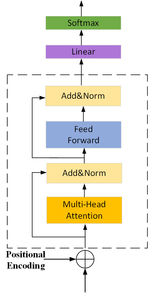
Figure 1.
Structure of the Transformer Encoder.
The structure of the multi-head self-attention mechanism is shown in Figure 2. This part computes the correlation weights between each element in the input sequence and the other elements, then performs a weighted sum of the information in the sequence to obtain the output feature sequence. Specifically, given an input feature sequence X, the multi-head attention mechanism uses a set of learnable parameter matrices to map the input features into H sets of query, key, and value matrices through H linear transformations. The query matrix represents the information that is used to compute how relevant each element in the sequence is to others, essentially asking which parts of the sequence are important for a particular element. The key matrix represents the content of each element that can be compared with the query to determine the relationship. The value matrix holds the actual information from the sequence that is aggregated based on the attention weights calculated between queries and keys. In multi-head attention, a head refers to one set of these query, key, and value matrices, allowing the model to simultaneously focus on different parts of the sequence. The results from each head are then concatenated and passed through a final linear transformation to produce the output sequence.
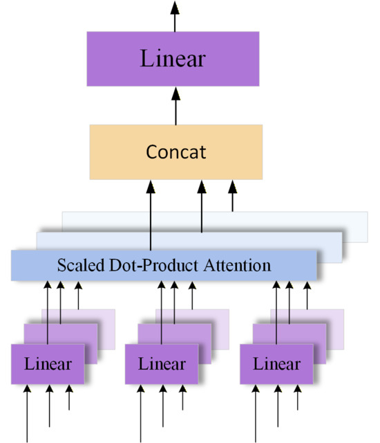
Figure 2.
Structure of the Multi-Head Self-Attention Mechanism.
Then, based on these three matrices, the normalized dot-product attention weighted features are calculated for each head. The model adopts 6 attention heads, 3 encoder layers, and a feed-forward network dimension of 480. The above computation process can be represented as:
where
,
, and
represent the query, key, and value matrices for the h-th attention head, and
,
, and
denote the learnable parameter matrices corresponding to the h-th attention head.
represents the weighted features of the h-th attention head, and d is the dimension of each feature vector.
Finally, the output features from all H attention heads are concatenated, and the concatenated result is mapped back to the original data space through a linear transformation matrix
, in order to achieve information integration and dimensional alignment. The computation process can be represented as:
where “Concat” denotes the feature concatenation operation, and
represents the learnable parameter matrix.
After extracting features through the Transformer encoder, we obtain a high-dimensional feature representation Z∈
, where 40 represents the number of flight instructors, T is the number of time steps, and D is the dimension of the encoder’s hidden layer (D = 120). From the above process, it can be seen that the high-dimensional features are generated through three steps. First is input processing: each flight instructor’s 5-dimensional time series data (IAS, AltMSL, VSpd, Pitch, TRK, of shape T × 5) is mapped to a hidden dimension of D = 120 through a linear mapping layer. Next, the mapped sequences are passed through multiple layers of Transformer Encoders, preserving the time-step dimension T. Finally, the independently processed data of all 60 flight instructors are stacked together to form a tensor of shape 60 × T × D.
To generate a standardized multi-dimensional time series, we perform average pooling across the encoded results of all 60 time series. For each time step t, we compute the average encoding feature across the 60 time series at that time step:
where
represents the encoding feature of the i-th time series at the t-th time step. Through the average pooling operation, we obtain a standardized time series of shape T × D.
To map it back to the original 5-dimensional space, we use a fully connected layer for feature mapping. The computation process is as follows:
where
is the weight matrix of the linear layer, and
is the bias vector of the linear layer.
Through this linear mapping operation, we map the original input data of dimension D to the 5 flight parameters (altitude, indicated airspeed, vertical speed, pitch angle, and heading angle), ultimately obtaining a standardized multi-dimensional time series of shape T × 5. This sequence can serve as the reference template for subsequent DTW similarity measurements.
2.4. DTW Similarity Measurement Based on Mahalanobis Distance
The process of time series similarity measurement is carried out using the DTW algorithm. DTW is a classical algorithm used to measure the similarity between time series. The core idea of this method is to use dynamic programming to find the optimal nonlinear alignment path between two time series, thereby overcoming the limitation of traditional Euclidean distance, which requires strict alignment along the time axis [39,40]. Given two time series X =
and Y =
, where n and m are the lengths of the two sequences, the DTW algorithm constructs an n × m distance matrix D:
In the formula,
represents the local distance between
and
, where
and
are the n-th element of sequence X and the m-th element of sequence Y, respectively. The dynamic programming method is used to find the optimal alignment path W between the two sequences, where W =
, and
is the k-th element in the alignment path, with k ranging from max(m,n) to m + n − 1. The DTW method is then used to calculate the optimal matching path between the two sequences, yielding the minimum dynamic time warping distance, as shown in the following formula:
In the formula, D(x,y) represents the DTW distance between sequences X and Y.
Mahalanobis distance is a multi-dimensional distance measurement method. This approach introduces a covariance matrix, which effectively considers the correlations between features, addressing the issue that Euclidean distance cannot account for feature correlations in multi-dimensional spaces. Given sequence matrices A = [a1,a2,…,an] and B = [b1,b2,…,bm], the Mahalanobis distance between the two sequences is defined as follows:
In the formula, S−1 represents the inverse of the full-rank covariance matrix, also known as the Mahalanobis matrix. The calculation of Mahalanobis distance involves using the linear transformation of the matrix to map the original feature space to a new feature space with improved metrics, thereby effectively measuring the distance between the two sequences. The traditional DTW algorithm based on Euclidean distance, as described earlier, can only measure the distance between unidimensional time series and cannot effectively handle the issue of multi-dimensional time series similarity measurement. Therefore, a DTW similarity measurement method based on Mahalanobis distance is proposed to meet the requirements of multi-dimensional time similarity measurement. Given two multi-dimensional time series XX and YY, the method is as follows:
In this context, d represents the dimensionality of the multi-dimensional time series, while m and n denote the lengths of X and Y, respectively. Define Xi = (x1i,x2i,…,xdi)T as the i-th column of X, which represents the values of all parameters at the i-th time point, and Yj = (y1j,y2j,…,ydj)T as the j-th column of Y, representing the values of all parameters at the j-th time point. The Mahalanobis distance is used to replace the Euclidean distance for calculating the local distance in DTW:
The covariance matrix S in this study is derived from the 5-dimensional time series data of 60 flight instructors. Ultimately, the DTW distance between the multi-dimensional time series X and Y, based on the Mahalanobis distance, is calculated as:
This distance represents the disparity between the multi-dimensional time series of each trainee and the standard multi-dimensional time series generated by the 60 competent instructors. A smaller distance value indicates a smaller difference from the standard sequence, suggesting better landing performance by the trainee.
2.5. Landing Quality Evaluation Based on K-Means Clustering
In this study, the K-means algorithm is used to cluster the similarity measures, which is a commonly employed unsupervised algorithm [41]. The reasons for selecting the K-means clustering method are as follows. Firstly, K-means, as a partition-based clustering algorithm, is renowned for its exceptional computational efficiency and favorable scalability. Secondly, based on expertise in the aviation field, we anticipate that the landing operation data of pilot groups with different skill levels tend to form compact, hyper-spherical clusters of similar sizes in the feature space. K-means, by minimizing the within-cluster sum of squares, naturally tends to discover clusters of this shape. Lastly, each cluster generated by K-means is represented by a clear centroid, which can be interpreted as the “typical” landing operation pattern for that category of pilots. This concise concept of “one central point representing one group” is easier to understand and apply. Given an DTW distances, the K-means algorithm performs clustering by minimizing the within-cluster sum of squares. During each iteration, the distance between the data points and the cluster centroids is calculated, and the data points are assigned to the cluster with the closest centroid. The centroid is then updated by calculating the mean of all the data points in the cluster. The algorithm process is illustrated in Figure 3. A K-means clustering analysis is performed based on the similarity metric values. The most important parameter of the K-means algorithm is the value of K. Before clustering the trainee data, both the elbow method and the silhouette score analysis were employed to determine the optimal number of clusters (K). The elbow method identifies the point where the rate of decrease in within-cluster sum of squares (WCSS) begins to slow down, while the silhouette score quantifies how well each data point fits its assigned cluster, with values ranging from −1 to 1 (higher values indicating better clustering quality).
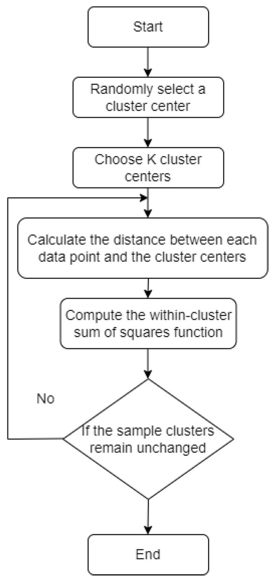
Figure 3.
Flowchart of the K-means Algorithm.
By using the K-means algorithm, the landing performance of the flight trainees is grouped into different clusters, with each group representing a specific level of landing quality, thereby enabling an overall evaluation of the trainees’ landing performance.
When calculating the DTW distance based on Mahalanobis distance, the contribution of each flight parameter is analyzed by calculating the difference between each pair of points in the standard time series and the trainee’s flight sequence using the weakness parameter identification method. The purpose of calculating the parameter contribution is to determine which flight parameters have the greatest impact on the differences between sequences. The specific steps are as follows: First, calculate the difference between each pair of matching points. To quantify the differences and prevent positive and negative differences from canceling each other out, the differences are squared. Then, the contributions of all time points are summed to obtain the total contribution of each flight parameter. At this point, without normalization, the contribution of different flight parameters may be unfairly compared due to differences in their dimensional units and numerical ranges. Therefore, the contribution of each flight parameter is normalized to ensure a fair comparison on the same scale.
3. Results and Discussion
3.1. Quality Clustering and Weak Parameter Identification Results
The flight data of 200 trainees, extracted from the SD card, are measured from the maximum descent angle to the maximum ascent angle. These data are then compared with a standard time series to assess their similarity. A partial list of the similarity measures is shown in Table 4.
Table 4.
Partial Time Series Similarity Metric Value for Selected Trainees.
The relationship between the WCSS (Within-Cluster Sum of Squares) value and K is shown in Figure 4. “WCSS” stands for Within-Cluster Sum of Squares, which is used to measure the sum of squared distances between data points and their respective cluster centroids.
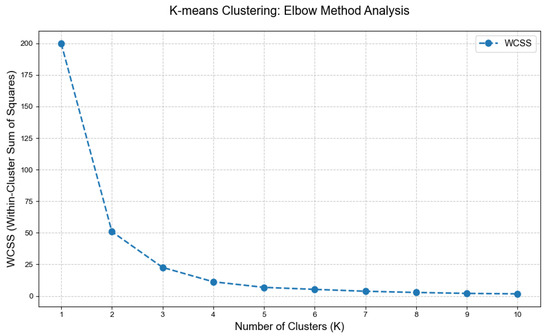
Figure 4.
Relationship between WCSS and K Value in the Elbow Method.
As shown in Figure 4, the inertia value decreases gradually with the increase in K. The objective is to identify an inflection point on the curve, where the reduction in inertia begins to slow down with the increase in the number of clusters. When K is around 4, the slope of the curve starts to flatten. Furthermore, the silhouette coefficients for different K values were calculated to quantitatively validate the clustering quality. As shown in Figure 5, K = 4 achieves the highest silhouette score of 0.6332, confirming it as the optimal number of clusters. Therefore, based on the elbow criterion, K = 4 is selected as the optimal number of clusters for the dataset. The clustering result based on time series similarity measure values when K = 4 is shown in Figure 6.
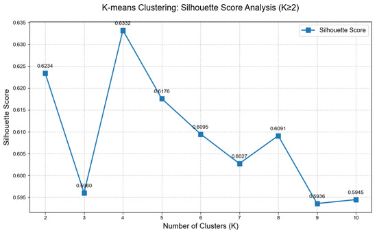
Figure 5.
Different K values correspond to silhouette coefficients.
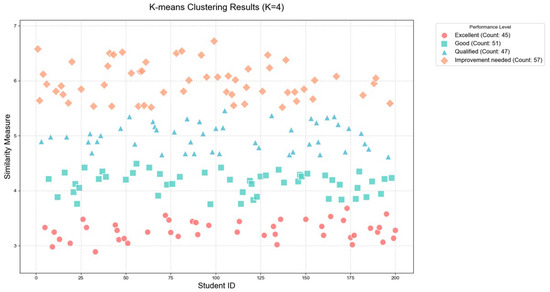
Figure 6.
Clustering Results of Trainee Landing Quality.
From the classification results shown in the figure, the landing performance of flight trainees can be divided into four categories: Excellent, Good, Qualified, and Improvement needed. It can be observed that 45 (22.5%) trainees have an excellent landing performance, 51 (25.5%) trainees have a good landing performance, 47 (23.5%) trainees have a qualified landing performance, and 57 (28.5%) trainees’ performance needs to be improved. Most of the flight trainees’ landing performance is at or above the qualified level. To assess differences between clusters, we performed one-way ANOVA, which revealed highly significant inter-group differences (F (3, 196) = 1098.64, p < 0.0001). Subsequent Tukey’s HSD post hoc tests further demonstrated significant pairwise differences among all cluster groups (all p < 0.0001). Descriptive statistics showed the expected gradient in similarity metric values: Excellent (M = 3.28, SD = 0.19) < Good (M = 4.14, SD = 0.20) < Qualified (M = 4.99, SD = 0.24) < Improvement Needed (M = 5.99, SD = 0.33). These results strongly validate the effectiveness of cluster analysis in distinguishing between trainees’ technical skill levels.
For trainees who are not rated as excellent, targeted training improvement suggestions should be provided. The evaluation results and weak parameters for some trainees are shown in Table 5.
Table 5.
Evaluation Results and Weak Parameters for Some Trainees.
3.2. Comparative Analysis and Discussion of Consistency with Instructor Ratings
To validate the effectiveness of the aforementioned data-driven quality assessment method, it is necessary to systematically compare its results with the subjective evaluations of flight instructors. From the current instructor rating system, landing performance scores based on a 5-point scale can be extracted, where 1 represents the poorest performance and 5 represents the best. The correspondence between the four relative levels derived from cluster analysis and the instructor ratings is shown in Table 6. The following analysis is conducted: score distribution, ranking consistency, and specific discrepancies.
Table 6.
Algorithm Clustering Results vs. Instructor Ratings.
Score Distribution Analysis: Instructor ratings were concentrated in the 3–5 point range. This distribution arises because the selected trainees had all passed the private pilot license screening phase, meaning instructors considered them to have mastered basic flight skills. Scores of 1 and 2 represent absolute failure and are thus rarely assigned, reflecting an absolute standard of pass/fail. In contrast, the algorithm performed classification based on the relative performance within this specific cohort of 200 trainees, resulting in a more uniform distribution across the four levels, which reflects a relative standard of distinction.
Ranking Consistency Analysis: The Spearman rank correlation coefficient was 0.71 (p < 0.001). This indicates a high level of consistency in the relative ranking of trainee performance between the algorithm and the instructors, despite the differences in their scoring systems.
Discrepancy Analysis:
- The primary disagreement centered on the algorithm’s “Improvement Needed” group. All trainees in this group received instructor ratings of 3 or 4, rather than the failing scores of 1 or 2. This stems from the differing evaluation logics: the algorithm identified them as the relatively weakest within the cohort, whereas the instructors deemed them to have met the absolute minimum requirements of the curriculum. While the operational techniques of these trainees likely satisfied all key qualification criteria in the Training Syllabus from an absolute pass/fail standpoint, the algorithm acutely revealed their relative disadvantage within the group. This provides precise targets for instructional intervention, preventing their technical shortcomings from being masked by a “pass” label.
- The average instructor rating for the “Improvement Needed” group (3.59) was higher than that for the “Qualified” group (3.26), further illustrating the difference in assessment logic. Although algorithmically classified as relatively weaker performers, the majority of trainees in the “Improvement Needed” group (33 individuals) were rated by instructors as having met the absolute standard for “Good” (score of 4), thereby elevating the group’s average score. This discrepancy is further accentuated by the differing evaluation scopes: instructors’ comprehensive assessments include the ground roll phase, while the algorithmic analysis is confined solely to the landing flare phase. This clearly demonstrates the algorithm’s capability to reveal relative technical deficiencies during the landing flare phase that remain concealed under the absolute evaluation framework. Even when instructors assign a “Good” rating to trainees in the “Improvement Needed” group, the algorithm accurately identifies them as requiring prioritized assistance within the cohort.
- Cases where trainees received favorable algorithmic ratings but lower instructor evaluations are also noteworthy. Specifically, we identified 10 trainees algorithmically rated as “Good” but instructor-rated as 3 (“Qualified”)—the most typical “algorithm-high, instructor-low” cases. From the algorithm’s perspective, their landing operations showed moderate deviation from the standard sequence (similarity metric ~3.75–4.49), placing them in the upper-middle tier of the cohort. However, instructors judged their performance as merely “Qualified”. Furthermore, 16 trainees were rated “Excellent” by the algorithm but only “Good” (rating 4) by the instructors. These algorithmically top-tier trainees (similarity metric ~2.89–3.68) did not receive the highest instructor rating. A key reason is that instructor evaluations encompass the entire landing phase, including the ground roll, and incorporate assessment criteria beyond technical manipulation, such as Crew Resource Management skills (e.g., communication, workload management). The algorithmic clustering, in contrast, is based solely on flight parameters, excludes non-technical skills, and does not include the ground roll phase. Therefore, for these algorithmically “Excellent” trainees, the lower instructor rating might be due to deficiencies in non-technical factors like passive communication, less satisfactory performance during the ground roll, or potentially higher standards and expectations held by the instructors, who thus refrain from awarding the top score.
Compared to traditional instructor evaluation, the algorithmic assessment, based on objective flight parameter data and relative ranking, effectively mitigates interference from subjective factors. It identifies trainees who, despite meeting the absolute pass standard, still require technical improvement. This data-driven method demonstrates higher sensitivity and discriminative power, enabling precise identification of specific skill gaps during particular training phases and providing reliable quantitative evidence for targeted training intervention. However, instructor evaluation offers a more comprehensive assessment perspective, effectively capturing non-technical skills that are difficult for the algorithm to quantify. Therefore, integrating the algorithmic assessment proposed in this study with instructor evaluations can provide a reference for constructing a more robust and comprehensive assessment system.
3.3. Individual Case Analysis Using Parameter Curves
By combining visual analysis, we plot the similarity curves of the trainee’s parameters and the standard template parameters after time-step alignment on the same graph. Each curve represents the temporal variation in a specific parameter. By comparing the trainee’s curve with the standard template curve, deviations between the trainee and the standard template at different time points can be identified. The trend of the trainee’s curve is compared to that of the standard template curve to observe whether they align. If a trainee’s parameter exhibits significant fluctuations or deviates considerably from the standard template at a certain time point, it indicates weaker performance during that period. Ultimately, based on the differences between the trainee’s and the standard template’s parameters, a personalized training plan can be tailored to the trainee to ensure that the flight parameters at different time points are as close as possible to the standard template. The comparison of a specific trainee’s parameters with the standard template parameters is shown in Figure 7, Figure 8, Figure 9, Figure 10 and Figure 11 below.
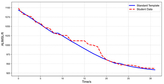
Figure 7.
Comparison of Altitude Similarity Curves for a Specific Trainee.
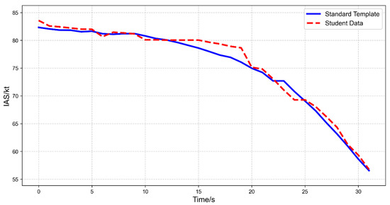
Figure 8.
Comparison of Indicated Airspeed Similarity Curves for a Specific Trainee.
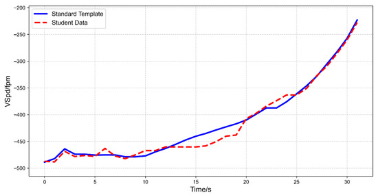
Figure 9.
Comparison of Vertical Speed Similarity Curves for a Specific Trainee.
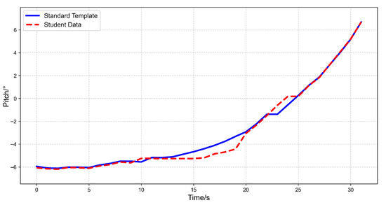
Figure 10.
Comparison of Pitch Angle Similarity Curves for a Specific Trainee.
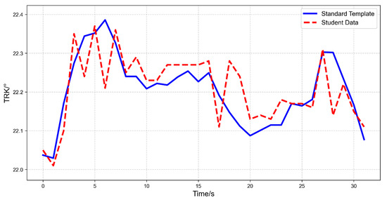
Figure 11.
Comparison of Track Angle Similarity Curves for a Specific Trainee.
The horizontal axis in the figure represents time, where the zero point (0 s) corresponds to the initiation of the transition from the final approach attitude to the landing attitude, extending until main gear touchdown (30 s). The vertical axis represents various flight parameters. Figure 7 presents a comparison between the altitude profile of a specific student and the instructor’s standard template during the final 30 s before landing. It clearly shows that while the instructor’s standard template exhibits a smooth trajectory, the student’s profile displays noticeable altitude fluctuations between 12–20 s. Figure 8 shows a comparison between the airspeed profile of a trainee and the instructor’s standard template during the final 30 s before landing. It can be observed that while the instructor’s standard airspeed profile remains relatively smooth, the trainee exhibits noticeable airspeed fluctuations between 15–20 s. Figure 9 presents a comparison between the vertical speed profile of a trainee and the instructor’s standard template during the final 30 s before landing. It clearly shows that around the 18 s mark, the vertical speed suddenly increases significantly. Figure 10 displays a comparison between the pitch angle profile of a trainee and the instructor’s standard template during the final 30 s before landing. It clearly shows that the pitch angle gradually increases over time, reaching approximately 6 degrees at the moment of touchdown. Figure 11 compares the temporal differences in track angle control between a specific trainee and the standard template.
From the comparison of the similarity curves above, it can be observed that, compared to the standard template, the trainee’s performance in the 15 s prior to touchdown is suboptimal, with larger fluctuations in indicated airspeed and vertical speed, and with higher indicated airspeed and pitch angle, while vertical speed is lower. The trainee’s vertical speed deviates the most from the standard template curve, indicating that vertical speed is the weakest flight parameter. Therefore, during subsequent flight training, the trainee should focus on controlling indicated airspeed and pitch angle in the 15 s before touchdown, and specifically train their ability to manage vertical speed in order to achieve a smooth landing.
These deviations could pose multiple risks. Precise airspeed management is a critical factor in ensuring safety. Excessively high airspeed at touchdown can cause the aircraft to “float” due to excessive residual lift, significantly delaying the touchdown point. This not only consumes more runway length but may also lead to tire bursts or directional control loss during deceleration due to emergency braking, potentially resulting in a runway excursion. Conversely, excessively low airspeed approaches the stall boundary, causing a sharp deterioration in aircraft controllability and making the aircraft prone to sudden sinking and hard landings when encountering turbulence. Simultaneously, pitch angle control is equally crucial: an excessively high pitch angle during the flare phase rapidly increases the angle of attack, potentially triggering a stall at low altitude. This could cause the aircraft to lose lift and impact the runway heavily, potentially damaging the landing gear and airframe structure, or even causing a tail strike. An excessively low pitch angle indicates failure to establish an effective landing attitude, leading to excessive impact force on the main gear or premature nose gear contact. Additionally, vertical sink rate control is particularly important for fixed landing gear. Even a seemingly moderate excessive sink rate may subject the aluminum alloy landing gear structure to overload, causing structural deformation or component cracks. Hard landings may also induce porpoising phenomenon and undermine the trainee’s control confidence. Therefore, training should emphasize strengthening the trainee’s ability to accurately maintain target speed through coordinated throttle and pitch operations, control pitch changes through smooth and consistent control inputs, and develop the skill to actively perceive sink changes during the flare phase, using subtle and consistent pull-up inputs to gradually stabilize the descent rate. Quantitative evaluation based on these flight parameters can effectively diagnose operationally significant control deficiencies, providing clear and objective scientific basis for instructors to develop targeted training programs.
Our research has achieved the capability to diagnose operational deficiencies through quantitative evaluation of flight parameters, providing scientific basis for personalized training programs. Future research could consider quantifying group-level technical deviations by deconstructing the sub-costs of individual parameters in the multivariate DTW calculation, which would enable precise quantification of the extent to which trainees deviate from instructor standards in key variables such as airspeed, pitch angle, and vertical speed, thereby facilitating the identification of common technical bottlenecks. Furthermore, based on the existing clustering results, we can identify stable, frequently co-occurring parameter deviation combinations within specific groups—such as the characteristic “high-pitch, low-airspeed”—to summarize typical error patterns and provide more precise guidance for flight training.
4. Conclusions and Future Work
This study has established a landing quality assessment framework based on SD card data and time-series similarity analysis for the DA40NG aircraft. Compared with existing research, the innovation of this method is mainly reflected in three aspects: by systematically integrating the complete time series of five key flight parameters, a multi-dimensional dynamic evaluation of the flare phase was achieved; the combination of the Transformer encoder and the Mahalanobis distance-based DTW algorithm effectively solved the similarity measurement problem of multivariate time series; a complete assessment chain from data collection to personalized training suggestions was established.
The results demonstrate a significant consistency (Spearman correlation coefficient 0.71) between the proposed method and the instructor evaluation system under the specific operational environment of a designated training airport, confirming the effectiveness of the data-driven approach in flight skill assessment. More importantly, the systematic discrepancies between the algorithmic and instructor evaluations reveal their complementary value: the algorithm can acutely identify subtle deviations in technical parameters, while instructors can comprehensively consider non-technical factors. This complementary relationship provides new insights for constructing a human–machine collaborative evaluation system. However, this study still has several limitations that need to be addressed in future research.
- (1)
- Scope Limitations: Data collection for this study was confined to a single aircraft type and a single airport, with meteorological conditions filtered to control for external variables. While this design facilitates focused analysis of trainees’ fundamental maneuvering skills during the initial research phase, the generalizability and broader applicability of the conclusions require further validation. Future work will aim to expand the scope by incorporating multiple aircraft types, diverse airport characteristics (e.g., runway length), and varied meteorological conditions (e.g., crosswind conditions) to build a more robust evaluation system that meets the complex demands of actual flight training.
- (2)
- Relativity of Evaluation Criteria: It is important to note that the primary contribution of this study lies in providing an objective, quantifiable, data-driven evaluation framework. This framework can precisely identify a trainee’s relative position within the cohort and their individual weaknesses, which is highly valuable for personalized training guidance. However, this study essentially constitutes a relative assessment method based on a specific trainee population. The evaluation results reflect a trainee’s relative standing within the group rather than an absolute benchmark of skill. Therefore, the current assessment outcomes should be integrated with the qualitative evaluations of flight instructors to form a more comprehensive and fair judgment. This method is more suitable for the horizontal comparison and stratification of trainees within the same training batch, enabling the precise allocation of training resources, rather than for the absolute measurement of trainee capability across different training cycles. To enhance long-term repeatability and comparability of assessments, future work will focus on accumulating large-scale data to establish standardized benchmark norms.
Author Contributions
X.D.: Writing—review and editing, Supervision, Resources, Project administration, Funding acquisition, Formal analysis, Conceptualization. G.X.: Writing—original draft, Software, Data curation. Q.Y.: Methodology, Investigation. Y.X.: Methodology, Investigation, Visualization. B.C.: Writing—review and editing, Supervision, Methodology, Investigation, Funding acquisition, Formal analysis. All authors have read and agreed to the published version of the manuscript.
Funding
The study was funded by China Association of Transport Education (Key Project of Educational Science Research, 2024–2026, Grant No. JT2024ZD016), Key Project of Natural Science Foundation for Central Universities (Grant No. 3122025105).
Data Availability Statement
The data that support the findings of this study are available from the corresponding author upon reasonable request.
Conflicts of Interest
Author Qingkui Yang was employed by the company Tianjin Jeppesen International Flight College Co., Ltd. The remaining authors declare that the research was conducted in the absence of any commercial or financial relationships that could be construed as a potential conflict of interest.
References
- Boeing. Pilot & Technician Outlook 2023–2042; Boeing Commercial Market Outlook: Seattle, WA, USA, 2023; Available online: https://www.boeing.com/commercial/market/pilot-technician-outlook/ (accessed on 19 September 2025).
- Li, J.; Sun, H.; Li, F.; Cao, W.; Hu, H. Non-technical Competency Assessment for the Initial Flight Training Based on Instructor Measurement Data. In Proceedings of the 2nd International Conference on Big Data Engineering and Education (BDEE 2022), Shanghai, China, 5–7 August 2022; pp. 1–7. [Google Scholar] [CrossRef]
- Liu, H.; Wang, H.; Meng, G.L.; Wu, H.; Zhou, M. Flight Training Evaluation Based on Dynamic Bayesian Network and Fuzzy Grey Theory. J. Aeronaut. 2021, 42, 243–254. [Google Scholar] [CrossRef]
- Li, Q.; Du, D.; Cao, W.; Qian, J. A Quality Evaluation Model for Approach in Initial Flight Training Utilizing Flight Training Data. In Proceedings of the 2023 International Conference on Computer Applications Technology, CCAT, Guiyang, China, 15–17 September 2023; pp. 36–40. [Google Scholar] [CrossRef]
- Sun, H.; Zhou, X.; Zhang, P.; Liu, X.; You, L. Research on the Evaluation of Flight Manipulation Quality in Cloud Penetration Procedure Training. Flight Mech. 2023, 41, 88–94. [Google Scholar] [CrossRef]
- Liu, L.; Zhang, T.; Ru, B. Establishment of a Flight Quality Evaluation Model Based on Multi-parameter Fusion. Comput. Eng. Sci. 2016, 38, 1262–1268. [Google Scholar]
- Wang, S.; Chen, Y.; Zeng, C. A Flight Training Quality Evaluation Model Based on Over-limit Events. Sci. Technol. Eng. 2022, 22, 5074–5080. [Google Scholar]
- Wang, L.; Zhang, J.; Dong, C.; Sun, H.; Ren, Y. A Method of Applying Flight Data to Evaluate Landing Operation Performance. Ergonomics 2019, 62, 171–180. [Google Scholar] [CrossRef]
- Li, F.; Xu, X.; Li, J.; Hu, H.; Zhao, M.; Sun, H. Wind Shear Operation-Based Competency Assessment Model for Civil Aviation Pilots. Aerospace 2024, 11, 363. [Google Scholar] [CrossRef]
- Liu, W.; Liu, Y.; Yang, Y. Research on Quantitative Evaluation Methods for Flight Technology Combining Artificial Intelligence and Data. Aviat. Eng. Prog. 2025, 16, 171–182. Available online: http://kns.cnki.net/kcms/detail/61.1479.V.20240823.0908.002.html (accessed on 19 September 2025).
- Lu, F.; Wei, X.; Chen, H. Research on the Comprehensive Evaluation System of Civil Aviation Pilot Landing Operation Quality. J. Saf. Environ. 2025, 25, 558–571. [Google Scholar] [CrossRef]
- Smrz, V.; Boril, J.; Vudarcik, I.; Bauer, M. Utilization of recorded flight simulator data to evaluate piloting accuracy and quality. In Proceedings of the NTinAD 2019-New Trends in Aviation Development 2019-14th International Scientific Conference, Chlumec nad Cidlinou, Czech Republic, 26–27 September 2019; pp. 164–169. [Google Scholar] [CrossRef]
- Sun, B.; Shi, Z.; Pan, X.; Yan, Y.; Wang, F. Aircraft Flight Quality Evaluation Based on Grey Relational Analysis and XGBoost. Aviat. Eng. Prog. 2025, 16, 74–81. Available online: http://kns.cnki.net/kcms/detail/61.1479.V.20240701.1402.004.html (accessed on 19 September 2025).
- Yuan, W.L.; Lu, C.Y.; Lu, W.; He, S. Flight Quality Evaluation Based on Machine Learning. Sci. Technol. Eng. 2021, 21, 8262–8269. [Google Scholar]
- Shang, L.; Wang, H.; Si, H.; Wang, Y.; Pan, T.; Liu, H.; Li, Y. Flight Trainee Performance Evaluation Using Gradient Boosting Decision Tree, Particle Swarm Optimization, and Convolutional Neural Network (GBDT-PSO-CNN) in Simulated Flights. Aerospace 2024, 11, 343. [Google Scholar] [CrossRef]
- Li, G.; Wang, H.; Si, H.; Pan, T.; Liu, H. Research on the construction of flight skill evaluation model for flight students based on T-S fuzzy neural network. Manned Spacefl. 2023, 29, 616–623. [Google Scholar] [CrossRef]
- Tian, W.; Zhang, H.; Li, H.; Xiong, Y. Flight maneuver intelligent recognition based on deep variational autoencoder network. Eurasip J. Adv. Signal Process. 2022, 2022, 21. [Google Scholar] [CrossRef]
- Park, J.-C.; Jung, K.-W.; Kim, Y.-W.; Lee, C.-H. Anomaly Detection Method for Missile Flight Data by Attention-CNN Architecture. J. Inst. Control Robot. Syst. 2022, 28, 520–527. [Google Scholar] [CrossRef]
- Wang, S.; Liu, Z.; Jia, Z.; Tang, Y.; Zhi, G.; Wang, X. Fault Detection for UAVs With Spatial-Temporal Learning on Multivariate Flight Data. IEEE Trans. Instrum. Meas. 2024, 73, 2529517. [Google Scholar] [CrossRef]
- Knignitskaya, T.V. Estimate of time series similarity based on models. J. Autom. Inf. Sci. 2019, 51, 70–80. [Google Scholar] [CrossRef]
- Tan, C.W.; Herrmann, M.; Salehi, M.; Webb, G.I. Proximity forest 2.0: A new effective and scalable similarity-based classifier for time series. Data Min. Knowl. Discov. 2025, 39, 14. [Google Scholar] [CrossRef]
- Yin, J.; Wang, R.; Zheng, H.; Yang, Y.; Li, Y.; Xu, M. A New Time Series Similarity Measurement Method Based on the Morphological Pattern and Symbolic Aggregate Approximation. IEEE Access 2019, 7, 109751–109762. [Google Scholar] [CrossRef]
- Lv, J.; Shi, X.; Xiao, Z. Fault diagnosability evaluation method based on DTW timing distance. Acta Armamentarii 2024, 45, 997–1009. [Google Scholar] [CrossRef]
- Wei, H.; Yang, F.; Zhu, H.; Zhang, M.; Yin, H. Matching method of track dynamic and static inspection data based on DTW. J. Railw. Sci. Eng. 2022, 19, 78–86. [Google Scholar] [CrossRef]
- Li, C.; Zhang, Y.; Ji, W.; Si, X.; Li, X. Research on the Extraction and Recognition of Complex Flight Actions of Military Aircraft. Aviat. Weapons 2023, 30, 127–134. [Google Scholar] [CrossRef]
- Wan, J.; Yang, P.; Zhang, W.; Cheng, Y.; Cai, R.; Liu, Z. A taxi detour trajectory detection model based on iBAT and DTW algorithm. Electron. Res. Arch. 2022, 30, 4507–4529. [Google Scholar] [CrossRef]
- Qiao, M.; Liu, Y.; Tao, H. A similarity metric algorithm for multivariate time series based on information entropy and DTW. Zhongshan Daxue Xuebao/Acta Sci. Natralium Univ. Sunyatseni 2019, 58, 1–8. [Google Scholar] [CrossRef]
- Mei, J.; Liu, M.; Wang, Y.-F.; Gao, H. Learning a Mahalanobis Distance-Based Dynamic Time Warping Measure for Multivariate Time Series Classification. IEEE Trans. Cybern. 2016, 46, 1363–1374. [Google Scholar] [CrossRef] [PubMed]
- Dai, M. A hybrid machine learning-based model for predicting flight delay through aviation big data. Sci. Rep. 2024, 14, 4603. [Google Scholar] [CrossRef]
- Sun, H.; Zhou, X.; Zhang, P.; Liu, X.; Lu, Y.; Huang, H.; Song, W. Competency-based assessment of pilots’ manual flight performance during instrument flight training. Cogn. Technol. Work. 2023, 25, 345–356. [Google Scholar] [CrossRef]
- Zhou, S.; Zhou, Y.; Xu, Z.; Chang, W.; Cheng, Y. The landing safety prediction model by integrating pattern recognition and Markov chain with flight data. Neural Comput. Appl. 2019, 31 (Suppl. S1), 147–159. [Google Scholar] [CrossRef]
- Li, G.; Wang, H.; Pan, T.; Liu, H.; Si, H. Fuzzy Comprehensive Evaluation of Pilot Cadets’ Flight Performance Based on G1 Method. Appl. Sci. 2023, 13, 12058. [Google Scholar] [CrossRef]
- Hebbar, P.A.; Pashilkar, A.A. Pilot performance evaluation of simulated flight approach and landing maneuvers using quantitative assessment tools. Sadhana 2017, 42, 405–415. [Google Scholar] [CrossRef]
- Boeing Commercial Airplanes. Statistical Summary of Commercial jet Airplane Accidents: 2015–2024; Boeing: Seattle, WA, USA, 2024; Available online: https://www.boeing.com/content/dam/boeing/boeingdotcom/company/about_bca/pdf/statsum.pdf (accessed on 19 September 2025).
- International Civil Aviation Organization (ICAO). Accident Incident Data Reporting (ADREP) Taxonomy, 2020 Edition; ICAO: Montreal, QC, Canada, 2020; Available online: https://www.icao.int/safety/AIG/taxonomy (accessed on 27 October 2025).
- Guo, C.; Sun, Y.; Xu, T.; Hu, Y.; Yu, R. An Improved Transformer Method for Prediction of Aircraft Hard Landing Based on QAR Data. Int. J. Aeronaut. Space Sci. 2025, 26, 2043–2057. [Google Scholar] [CrossRef]
- Ayhan, B.; Vargo, E.P.; Tang, H. On the Exploration of Temporal Fusion Transformers for Anomaly Detection with Multivariate Aviation Time-Series Data. Aerospace 2024, 11, 646. [Google Scholar] [CrossRef]
- Vaswani, A.; Shazeer, N.; Parmar, N.; Uszkoreit, J.; Jones, L.; Gomez, A.N.; Kaiser, Ł.; Polosukhin, I. Attention Is All You Need. In Proceedings of the Advances in Neural Information Processing Systems 30 (NIPS 2017), La Jolla, CA, USA, 4–9 December 2017; 2017; pp. 5999–6009. [Google Scholar]
- El Amouri, H.; Lampert, T.; Gançarski, P.; Mallet, C. Constrained DTW preserving shapelets for explainable time-series clustering. Pattern Recognit. 2023, 143, 109804. [Google Scholar] [CrossRef]
- Ma, Y.; Tang, Y.; Zeng, Y.; Ding, T.; Liu, Y. An N400 identification method based on the combination of Soft-DTW and transformer. Front. Comput. Neurosci. 2023, 17, 1120566. [Google Scholar] [CrossRef]
- Sinaga, K.P.; Yang, M.-S. Unsupervised K-Means Clustering Algorithm. IEEE Access 2020, 8, 80716–80727. [Google Scholar] [CrossRef]


Disclaimer/Publisher’s Note: The statements, opinions and data contained in all publications are solely those of the individual author(s) and contributor(s) and not of MDPI and/or the editor(s). MDPI and/or the editor(s) disclaim responsibility for any injury to people or property resulting from any ideas, methods, instructions or products referred to in the content. |
© 2025 by the authors. Licensee MDPI, Basel, Switzerland. This article is an open access article distributed under the terms and conditions of the Creative Commons Attribution (CC BY) license (https://creativecommons.org/licenses/by/4.0/).