Deep Reinforcement Learning-Based Differential Game Guidance Law against Maneuvering Evaders

Abstract

To achieve the intelligent interception of different types of maneuvering evaders, based on deep reinforcement learning, a novel intelligent differential game guidance law is proposed in the continuous action domain. Different from traditional guidance laws, the proposed guidance law can avoid tedious manual settings and save cost efforts. First, the interception problem is transformed into the pursuit–evasion game problem, which is solved by zero-sum differential game theory. Next, the Nash equilibrium strategy is obtained through the Markov game process. To implement the proposed intelligent differential game guidance law, an actor–critic neural network based on deep deterministic policy gradient is constructed to calculate the saddle point of the differential game guidance problem. Then, a reward function is designed, which includes the tradeoffs among guidance accuracy, energy consumption, and interception time. Finally, compared with traditional methods, the interception accuracy of the proposed intelligent differential game guidance law is 99.2%, energy consumption is reduced by 47%, and simulation time is shortened by 1.58 s. All results reveal that the proposed intelligent differential game guidance law has better intelligent decision-making ability.

1. Introduction

With the development of intelligent information technology, advanced guidance laws play a crucial role in accurate interception missions. Furthermore, when confronting different types of maneuvering evaders, it is crucial for the pursuer to rapidly perceive the environment and generate a favorable, accurate, and effective guidance strategy. Therefore, intelligent guidance laws for intercepting maneuvering evaders have attracted the attention of many scholars.

Traditional guidance laws include proportional navigation guidance (PNG) [1], augmented proportional navigation guidance (APNG) [2], optimal guidance laws (OGLs) [3], and sliding mode control (SMC) guidance laws [4]. However, those methods are not intelligent and need many manual settings. Additionally, the evader is treated as a stationary object. As is well known, intercepting maneuvering evaders involves a game process known as the classical pursuit–evasion game. For solving the interception problem of maneuvering evaders, differential game (DG) theory shows its advantages, where the interception problem is transformed into finding the saddle point of Nash equilibrium. In [5], an intelligent guidance algorithm was proposed for effectively intercepting the maneuverable target by virtue of DG concepts. The engagement kinematics, in addition to the direct intercept condition, were developed with 2D engagement. In [6], linear quadratic differential game (LQDG) guidance laws were proposed for solving the two-pursuit versus single-evader problem. The interception strategy was derived from the Nash equilibrium strategy set of the game. Similarly, in [7], differential game guidance laws were proposed for a linear system. However, obtaining an analytic solution becomes nearly impossible as the system grows more complex.

To address the nonlinear problem, adaptive dynamic programming (ADP) techniques provide powerful tools to solve nonlinear DG problems. Value iteration and policy iteration are employed to solve differential game guidance laws (DGGLs). In [8], a data-driven value iteration (VI) algorithm was proposed to solve the adaptive continuous-time linear optimal output regulation, and the author designed an online value iteration algorithm to learn the feedback control gain. In [9], an online policy iteration algorithm was proposed to achieve infinite-horizon optimal design for nonlinear two-player zero-sum games. However, insufficient iterations within a fixed sampling time may lead to system instability. To address this problem, in [10], the author proposed a time-based neuro-dynamic programming (NDP) algorithm, where the previous history of system states and cost function approximations were considered to solve the iteration problem. In [11], three neural network approximators were designed to learn the cost function, and an online NDP algorithm was proposed to solve the two-player zero-sum game problem in a continuous-time (CT) system. However, these guidance laws are not autonomous intelligent strategies, indicating that guidance systems lack the attributes of intelligent decision-making systems.

With the development of ADP techniques, reinforcement learning (RL) is gaining more attention as an effective method for obtaining autonomous intelligent guidance strategies. In [12], reinforcement learning was applied to solve the differential game problem, and the minimax point was found using discrete iteration. In [13], the researchers investigated the use of reinforcement learning techniques, based on the Q-learning algorithm, to implement interception strategies. Moreover, in [14], based on Q-learning and the fuzzy inference system, a fuzzy logic controller was proposed for solving pursuit–evasion differential games. The proposed method could solve the maneuverability of the evader when it is unknown. In [15], Jun Jet Tai’s work on reinforcement learning algorithms demonstrates that PyFlyt enables the configuration of arbitrary UAV types, such as dog fighting in the open-source PyFlyt software (PyFlyt 4.0.0). However, these reinforcement learning algorithms were implemented by discretizing the continuous action domain, potentially leading to exponential growth in calculations. To address this problem, deep reinforcement learning (DRL), with its advantage in solving the continuous control problem, was considered. In [16], modified multiagent reinforcement learning was proposed to achieve the underwater target hunting task under the constraints of energetic flows and acoustic propagation delay. In [17], deep deterministic policy gradient (DDPG) techniques were applied in guidance applications, and an intelligent impact time guidance law with the field-of-view was proposed. The guidance gain was obtained by the DDPG framework, which maximizes the expected total reward. In [18], for solving the hypersonic pursuit–evasion game, an intelligent maneuver strategy was proposed based on the TD3 algorithm and a deep neural network; the proposed algorithm could explore potential maneuver manners. Similar work is discussed in reference [19]. Although these DRL guidance laws can solve the interception problem by maximizing the expected reward, the evader is regarded as part of the environment without intelligent decision. Furthermore, there exist almost no papers that study the differential game guidance law (DGGL) for solving the interception problem in a continuous domain by DRL.

This paper innovatively combines DRL technology with DG theory to solve the DDGL design in the continuous domain. An intelligent differential game guidance law (IDGGL) algorithm is proposed. The main contributions of this paper are emphasized as follows.

1. Unlike traditional guidance laws, the advantages of the proposed IDGGL are saving cost efforts and avoiding tedious manual settings. The guidance model is obtained directly from environmental interaction learning through reinforcement learning. It is an intelligent guidance strategy, which can save more simulation time.

2. The problem of differential game interception is transformed into a Markov game. In general guidance algorithms based on deep reinforcement learning, the evader’s strategy is not considered. Unlike traditional DRL algorithms, our method formulates the guidance problem as a differential game, which allows for more sophisticated strategies in adversarial scenarios. The proposed IDGGL algorithm aims to determine the minimax saddle point rather than maximize the return. In this way, the evader is traded as an intelligent agent. This is the first application for DRL to solve the differential game interception problem.

3. Unlike numerous research works on guidance algorithms based on deep reinforcement learning, in our paper, a complex reward function is considered; on the one hand, the designed reward function aligns better with practical applications; on the other hand, it makes the training process faster and the trained model more accurate. A reasonable reward function is designed, which emphasizes not only the terminal interception distance but also the energy consumption and interception distance in the interception process. Additionally, replay buffer stores, “soft” target networks, and normalization techniques are adopted to make the training process more efficient. Additionally, for practical application, the action space with an added noise process is considered.

The structure of this paper is organized as follows. In Section 2, the pursuit–evasion game problem and the core concepts and principles of RL are presented. The framework of the zero-sum differential Markov game and the proposed IDGGL are presented in Section 3. In Section 4, numerical experiments are carried out to evaluate the performance of the proposed IDGGL strategy. Section 5 presents some conclusions.

2. Problem Statement and Preliminaries

First, we present the formulation of the pursuit–evasion game. In this engagement, the pursuer tries to intercept the evader, while the evader tries to escape from the pursuer. Then, the core concepts and principles of RL are introduced.

2.1. The Formulation of the Pursuit–Evasion Game

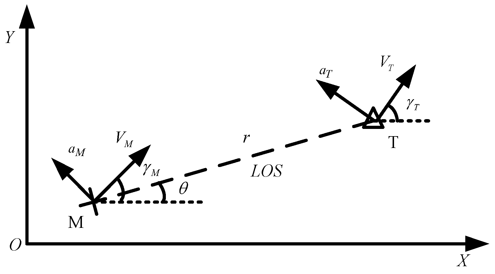
In this subsection, the engagement scenario in a plane is considered in Figure 1. The X-Y plane denotes the Cartesian reference frame. The variables $V_i\mathrm{a}\mathrm{n}\mathrm{d}{a}_i,i=(M,T)$ represent the velocity and the lateral acceleration of the pursuer and the evader, respectively. The variables ${\gamma }_M\mathrm{a}\mathrm{n}\mathrm{d}{\gamma }_T$ denote the flight path angles of the pursuer and the evader, respectively. $u_M\mathrm{a}\mathrm{n}\mathrm{d}{u}_T$ are the control inputs of the two players. We define the pursuer–evader relative distance and the line of sight (LOS) angle as r_d and θ.

In the terminal guidance stage, the interception time is very short; without loss of generality, the speeds of all agents are a constant speed. Thus, the interception curve appears to be a straight line. Then, the nonlinear kinematics of the pursuit–evasion game can be formulated as follows:

$$V_r=\dot{r_d}=V_{T}cos\left({\gamma }_T-\theta \right)-V_{M}cos\left({\gamma }_M-\theta \right)$$

(1)

$$\sigma =\dot{\theta }={(V}_{T}sin\left({\gamma }_T-\theta \right)-V_{M}sin\left({\gamma }_M-\theta \right))/r$$

(2)

where $V_r$ represents the closing velocity, and $\sigma$ donates the angular rate of the LOS.

In order to successfully intercept the evader, the concept of zero miss distance is used [5]. It can be defined as

$$\begin{array}{c}{z}_{miss}\left(t\right)=\frac{r^2\sigma }{\sqrt{{\dot{r}}^2+r^2{\sigma }^2}}\end{array}$$

(3)

It can be found that when the angular rate of the LOS approaches 0, the pursuer can intercept the evader. In general, there always exist external disturbances. Therefore, $x={\left[\theta \sigma \right]}^T$ are chosen as the states of the system [20]; by deriving Equation (2), accurate nonlinear dynamic equations can be obtained

$$\begin{array}{c}\dot{x}=f\left(x\right)-g\left(x\right)\left(a_m+d_m\right)+k\left(x\right)\left(a_t+d_t\right)\end{array}$$

(4)

where $f\left(x\right)={\left[0-\frac{2V_r}{r}\sigma \right]}^T$, $g\left(x\right)={\left[0\frac{cos\left({\gamma }_M-\theta \right)}{r}\right]}^T$, $k\left(x\right)={\left[0\frac{cos\left({\gamma }_T-\theta \right)}{r}\right]}^T$, and $d_m$ and $d_t$ are external disturbances. Generally, in practical applications, controllers are always affected by external disturbances, and considering the influence of external disturbances can make the training model more suitable for practical applications.

Traditionally, it is difficult to obtain the pursuer control command when the system has external disturbances. In this paper, the accurate nonlinear dynamics system is not required; we adopt the DRL technique to learn the interception strategy.

The first-order dynamics of the pursuer can be expressed as follows:

$${\dot{x}}_M=V_{M}cos{\gamma }_T$$

(5)

$${\dot{y}}_M=V_{M}sin{\gamma }_T$$

(6)

$${\dot{\gamma }}_M=\frac{a_m}{V_M}$$

(7)

$${\dot{a}}_M=\frac{u_M-a_m}{{\tau }_M}$$

(8)

where $(x_M,y_M)$ and $a_m$ are the position and the lateral acceleration of the pursuer, respectively. ${\tau }_M$ is a constant.

The first-order dynamics of the evader can be expressed as follows:

$${\dot{x}}_T=V_{T}cos{\gamma }_T$$

(9)

$${\dot{y}}_T=V_{T}sin{\gamma }_T$$

(10)

$${\dot{\gamma }}_T=\frac{a_t}{V_T}$$

(11)

$${\dot{a}}_T=\frac{u_T-a_t}{{\tau }_T}$$

(12)

where $(x_T,y_T)$ and $a_t$ are the position and the lateral acceleration of the evader, respectively. ${\tau }_T$ is a constant.

In the RL simulation, we utilized Equations (5)~(12) to achieve the motion of the pursuer and the evader. External disturbances were considered in the action space.

2.2. RL Framework

The basic principle of RL is that an agent interacts with the environment and learns a control policy, which can be described as a Markov Decision Process (MDP). The MDP consists of five elements $(S,A,P,r,\gamma )$, where $S$ denotes a set of states, $A$ is a set of actions, $P$ represents the state transition probabilities, $r$ is the reward function, and $\gamma$ denotes the optimal discount rate. In the MDP, at each timestep t, the agent interacts with the environment, receives a state $s_i\in S$, takes an action $a_i\in A$, and obtains a reward ${\gamma }_t$. Then, a trajectory $\{s_0,a_0,r_1,s_1,a_1,r_2\cdots \}$ is generated.

The goal in RL of the agent is to learn a control policy $\pi :S\to P\left(A\right)$, which describes states to a transition probability over the action. In general, the control policy $\pi$ can be learned by maximizing the return function, which is the sum of the future reward:

$$\begin{array}{c}R={\sum }_{i=t}^T{\gamma }^{i-t}r\left(s_i,a_i\right)\end{array}$$

(13)

The state-value function $V^{\pi }\left(s\right)$ and action-value function $Q^{\pi }\left(s,a\right)$ are used in many RL algorithms for obtaining the control policy $\pi$ [19]:

$$\begin{array}{c}{V}^{\pi }\left(s\right)=E_{\pi }\left({\displaystyle \sum _{i=0}^T}{\gamma }^{i}R\left(s_i\right)|s_0=S\right)\end{array}$$

(14)

$$\begin{array}{c}{Q}^{\pi }\left(s,a\right)=E_{\pi }({\displaystyle \sum _{i=0}^T}{\gamma }^{i}R\left(s_i,a_i\right)|s_0=S,a_0=A)\end{array}$$

(15)

where $E_{\pi }$ is the policy expected function. For the convenience of writing, $E_{\pi }$ is written as E in the following section.

For solving the continuous control problem, DRL shows its advantages. The basic idea of DRL involves adopting neural networks (NNs) to approximate the action-value function and state-value function. Typical algorithms in this domain include deep deterministic policy gradient (DDPG) and TD3. The main idea of these algorithms is that the state-value function and action-value function are parameterized by NNs. In this paper, we consider that the pursuer is continuously controlled.

3. Deep Reinforcement Learning Formulation of Differential Games

In this section, the pursuit–evasion game problem is considered as a zero-sum differential game. By combining Markov games and DRL, the IDGGL is proposed. Our emphasis is on two agents interacting with the environment and learning the Nash equilibrium strategy.

3.1. The Framework of the Zero-Sum Differential Markov Game

In the traditional Markov Decision Process (MDP), an agent interacts with the environment and maximizes the reward. Based on the MDP, the zero-sum differential Markov game is described by a tuple $(S,A_m,A_t,O,P,r,\gamma )$, where $S$ denotes the set of states. $A_m$ denotes the pursuer’s action space. $A_t$ represents the evader’s action space. $O$ is the set of observations. $P$ is the state transition probability $p\left(s_{t+1}|s_t,a_m,a_t\right).$ $R$ denotes the reward function of the agents. The reward function $r\left(s_t,a_m,a_t\right)$ describes the rewards that the pursuer acquires based on the actions of the evader. $\gamma \in \left(\mathrm{0,1}\right)$ represents the discount rate. In this paper, $S\ne O$; only the relative distance and LOS are observable during the process.

The behavior of the player is determined by a policy $\pi \left(s\right)$, which maps each state to an optimal action $s\to P\left(A_m,A_t\right).$ The evader’s actions can affect the optimal policy. The control strategy of the evader can be obtained through an observer. Thus, a rational pursuer knows the evader’s entire policy. Considering the impact of the evader’s strategies can make the learning model more suitable for practical applications. It is important to note that the policy may be stochastic, reflecting the stochastic nature of actions chosen by the evader and the environment. The goal of DRL is to learn a policy for two agents, who interact with a stochastic environment while finding the saddle point of the return function. The sum of the discounted future reward is defined as the return function, as follows:

$$\begin{array}{c}{R}_t={\sum }_{i=t}^T{\gamma }^{i-t}r\left(s_i,a_{mi},a_{ti}\right)\end{array}$$

(16)

where $\gamma \in \left[\mathrm{0,1}\right]$ represents the discount factor. $r\left(s_i,a_{mi},a_{ti}\right)$ is the designed reward function, which is presented in Section 3.3.

The expected total return is defined as the value function as follows:

$$\begin{array}{c}{Q}^{\pi }\left(s_t\right)=E\left(R_t|s_t\right)\end{array}$$

(17)

In the zero-sum differential Markov game, the pursuer tries to maximize the value function, while the evader has the contrary purpose that minimizes the value function.

$$\begin{array}{c}J={\underset{a_t\in A_t{a}_m\in A_m}{\mathrm{m}\mathrm{a}\mathrm{x}\mathrm{m}\mathrm{i}\mathrm{n}}Q}^{\pi }\left(s_t\right)\end{array}$$

(18)

According to the Bellman equation, the recursive relationship of the differential game value function yields

$$\begin{array}{c}{Q}^{\pi }\left(s_t\right)=E\left[R\left(s_t,a_m,a_t\right)\right]+\gamma Q^{\pi }\left(s_{t+1}\right)\end{array}$$

(19)

Unlikely traditional DRL, the zero-sum differential Markov game includes the evader’s strategy; the optimal policy of two agents is implemented by solving the following optimal value function

$$\begin{array}{c}{\pi }^{\ast }=(A_m^{\ast },A_t^{\ast })=\underset{\mathit{\pi }{\mathit{a}}_t\in A_{\mathit{t}}{a}_m\in A_m}{\arg \mathrm{max\; min}}{Q}^{\ast }\left(s_t\right)\end{array}$$

(20)

where ${\pi }^{\ast }$ is the optimal control variable of the pursuer and the evader. In the Markov game, the pursuer obtains the optimal control policy when the evader chooses the optimal control. In this paper, the pursuer learns the optimal interception policy when the evader chooses the optimal escape strategy. Thus, ${\pi }^{\ast }$ represents the control variables of two players in the game process.

In the DRL pursuit–evasion game, the pursuer will definitely learn the optimal control policy. In other words, the DRL algorithm will converge to the optimal value function $Q^{\ast }\left(s_t\right)$; the convergence of the DRL algorithm is given.

Theorem 1.

Under the framework of the zero-sum differential Markov game, the update rule of the value function is given as follows

$$\begin{array}{c}{Q}_{n+1}\left(s_t\right)=Q_n\left(s_t\right)+{\alpha }_{s_t}\left(r+\gamma \underset{{\mathit{a}}_t\in A_{\mathit{t}}{a}_m\in A_m}{\mathrm{maxmin}}{Q}_n\left(s_{t+1},a_{m+1},a_{t+1}\right)-Q_n\left(s_t\right)\right)\end{array}$$

(21)

where  ${\alpha }_{s_t}$  is the step-size and satisfies   $0{\le \alpha }_{s_t}\le 1$. Then, the DRL algorithm will converge to the optimal value function   $Q^{\mathrm{*}}\left(s_t\right)$, which corresponds to the optimal control policy.

Proof. 

First, we define the maximum error function as

$$\begin{array}{c}{∆}_n=\underset{}{\max }\left|Q_n\left(s_t\right)-Q^{\ast }\left(s_t\right)\right|\end{array}$$

(22)

where $Q_n\left(s_t\right)$ is the n-th step value function.

Then, Equation (19) can be rewritten as

$$\begin{array}{c}{Q}_{n+1}\left(s_t\right)=\left(1-{\alpha }_{s_t}\right)Q_n\left(s_t\right)+{\alpha }_{s_t}\left(r+\gamma \underset{{\mathit{a}}_t\in A_{\mathit{t}}{a}_m\in A_m}{\mathrm{maxmin}}{Q}_n\left(s_{t+1},a_{m+1},a_{t+1}\right)\right)\\ =\left(1-{\alpha }_{s_t}\right)Q_n\left(s_t\right)+{\alpha }_{s_t}{\Gamma Q}_n\left(s_t\right)\end{array}$$

(23)

where $\Gamma$ represents the Bellman operator.

Similarly, $Q^{\ast }\left(s_t\right)$ can be written as

$$\begin{array}{c}{Q}^{\ast }\left(s_t\right)=\left(1-{\alpha }_{s_t}\right)Q^{\ast }\left(s_t\right)+{\alpha }_{s_t}\Gamma Q^{\ast }\left(s_t\right)\end{array}$$

(24)

It is clearly noted that

$$\begin{array}{c}\left|{\Gamma Q}_n\left(s_t\right)-\Gamma Q^{\ast }\left(s_t\right)\right|\le \gamma \left|Q_n\left(s_t\right)-Q^{\ast }\left(s_t\right)\right|\end{array}$$

(25)

Subtracting Equation (21) from Equation (22) and combining Equation (23), we have

$$\begin{array}{c}\left|Q_{n+1}\left(s_t\right)-Q^{\ast }\left(s_t\right)\right|=\left|{\alpha }_{s_t}\left({\Gamma Q}_n\left(s_t\right)-\Gamma Q^{\ast }\left(s_t\right)\right)+\left(1-{\alpha }_{s_t}\right)\left(Q_n\left(s_t\right)-Q^{\ast }\left(s_t\right)\right)\right|\\ \le {\alpha }_{s_t}\left|{\Gamma Q}_n\left(s_t\right)-\Gamma Q^{\ast }\left(s_t\right)\right|+\left(1-{\alpha }_{s_t}\right)\left|Q_n\left(s_t\right)-Q^{\ast }\left(s_t\right)\right|\\ \le \left({\alpha }_{s_t}\gamma +\left(1-{\alpha }_{s_t}\right)\right){∆}_n\end{array}$$

(26)

Therefore, it can be concluded that the maximum $Q_{n+1}\left(s_t\right)$ is $\left({\alpha }_{s_t}\gamma +\left(1-{\alpha }_{s_t}\right)\right)$ times $Q_n\left(s_t\right)$. Let ${∆}_0$ represent the initial maximum error between $Q_0\left(s_t\right)$ and $Q^{\ast }\left(s_t\right)$. Then, upon the k-th iteration, the cumulative error can be obtained

$$\begin{array}{c}\left|Q_0\left(s_t\right)-Q^{\ast }\left(s_t\right)\right|\le {\left({\alpha }_{s_t}\gamma +\left(1-{\alpha }_{s_t}\right)\right)}^k{∆}_n\end{array}$$

(27)

□

Due to the fact that $0{\le \alpha }_{s_t}\le 1$, it can be concluded that $0\le \left({\alpha }_{s_t}\gamma +\left(1-{\alpha }_{s_t}\right)\right)\le 1$. Therefore, when $k\to \infty ,$ we have $\left|Q_0\left(s_t\right)-Q^{\ast }\left(s_t\right)\right|\le 0$. Thus, the DRL algorithm will converge to the optimal value function $Q^{\mathrm{*}}\left(s_t\right)$. In other words, when the pursuer learns the optimal policy, the closed-loop system of the pursuit–evasion game is stable.

Directly optimizing the value function or action-value function can obtain the optimal policy. However, this approach requires accurate model information. In practical applications, implementing such methods with model uncertainties can be challenging. Fortunately, model-free RL algorithms relax this requirement and find the optimal policy. One method to find the optimal policy is iteratively evaluating the value function, which is approximated by NNs. A well-known algorithm for this approach is the Q-learning algorithm. However, iterative approaches are typically limited to discrete action spaces. Another method involves policy gradient algorithms, which learn a deterministic function. In this approach, the action-value function is updated by the gradient direction of the value function with respect to the action. A well-known algorithm in this category is the DDPG algorithm [21], which can be applied in the continuous action domain. Thanks to this property, our proposed algorithm may solve the zero-sum differential game problem based on the framework of DDPG. The implementation is explained in the next section.

3.2. The Proposed Algorithm

For solving the zero-sum differential Markov game problem, an actor–critic NN framework is adopted based on the DDPG algorithm. In the zero-sum differential Markov game, our aim is to find the saddle point, which corresponds to learning the Nash equilibrium. The action-value function $Q(s,a_m,a_t)$ describes the return of the pursuer acquiring the maximum reward while the evader obtains the minimum reward. This function is approximated using the NN ${\theta }^Q(s,a_m,a_t)$ and parameterized by $Q$. The action-value function, commonly utilized in many RL algorithms, describes the expected return after taking actions $\left(a_m,a_t\right)$ in state $s_t$.

$$\begin{array}{c}{Q}^{\pi }\left(s_t,a_m,a_t\right)=E\left[R_t|s_t,a_m,a_t\right]\end{array}$$

(28)

According to the Bellman equation, the recursive relationship of the action-value function yields

$$\begin{array}{c}{Q}^{\pi }\left(s_t,a_m,a_t\right)=E\left[r\left(s_t,a_m,a_t\right)+\gamma E\left[Q^{\pi }\left(s_{t+1},a_{m+1},a_{t+1}\right)\right]\right]\end{array}$$

(29)

The action-value function is parameterized by ${\theta }^Q$; based on the temporal difference (TD) error, the loss function can be defined as follows:

$$L\left({\theta }^Q\right)=E{\left[{(Q}^{\pi }\left(s_t,a_t,a_t|{\theta }^Q\right)-y_t\right)}^2]$$

(30)

where

$$\begin{array}{c}{y}_t=r\left(s_t,a_t,a_t\right)+\gamma Q^{\mu }\left(s_{t+1},{\mu (s}_{t+1}\left)\right|{\theta }^Q\right)\end{array}$$

(31)

By minimizing the loss function, the parameter ${\theta }^Q$ is updated by using the gradient descent algorithm:

$$\begin{array}{c}{\theta }_{t+1}^Q={\theta }_t^Q-{\alpha }_{{\theta }^Q}{\nabla }_{{\theta }^Q}L\left({\theta }^Q\right)\end{array}$$

(32)

where ${\alpha }_{{\mathsf{\theta }}^{\mathrm{Q}}}$ is the learning rate of the critic network.

The inner expectation can be avoided by taking a deterministic policy. Thereafter, Equation (27) becomes the following:

$$\begin{array}{c}{Q}^{\mu }\left(s_t,a_m,a_t\right)=E\left[r\left(s_t,a_m,a_t\right)+\gamma Q^{\mu }\left(s_{t+1},{\mu (s}_{t+1},a_{m+1},a_{t+1})\right)\right]\end{array}$$

(33)

From Equation (31), it can be seen that the policy function depends only on the environment, which means $Q^{\pi }$ can be learned by using off-policy and transitions. Thus, the critic NN maps states to a specific action, which is parameterized by $\mu \left(s\right|{\theta }^{\mu })$. The update rule is to the expected return function $J$ with respect to the actor parameters:

$$\begin{array}{c}{\nabla }_{{\theta }^{\mu }}J=E\left[{\nabla }_{{\theta }^{\mu }}Q\left(s_t,a_m,a_t|{\theta }^Q\right){|}_{s=s_t,a_m,a_t=\mu \left(s_t|{\mu }^{\theta }\right)}\right]\\ =E\left[{\nabla }_{a_m,a_t}Q\left(s_t,a_m,a_t|{\theta }^Q\right){|}_{s=s_t,a_m,a_t=\mu \left(s_t\right)}{\nabla }_{{\theta }^{\mu }}\mu \left(s|{\theta }^{\mu }\right){|}_{\mathrm{s}=s_t}\right]\end{array}$$

(34)

where ${\nabla }_{(·)}$ represents the partial derivative of parameter $(·)$.

For the player, we expect maximizing the policy function. Therefore, the parameter ${\theta }^{\mu }$ is updated by using the policy gradient:

$$\begin{array}{c}{\theta }_{t+1}^{\mu }={\theta }_t^{\mu }+{\alpha }_{{\theta }^{\mu }}{\nabla }_{{\theta }^{\mu }}J\left({\theta }^{\mu }\right)\end{array}$$

(35)

where ${\alpha }_{{\mathsf{\theta }}^{\mathsf{\mu }}}$ is the learning rate of the actor network.

Remark 1.

In most optimization algorithms, samples are typically assumed to be independent and uniformly distributed. However, this assumption no longer holds when the samples are obtained from exploring sequentially in an environment. To address this problem, we adopt an experience replay buffer, as inspired by the DDPG algorithm. The finite replay buffer stores finite-sized transitions, denoted as$B_t=\left(s_t,a_t,o_t,r_t,s_{t+1}\right)$, which are sampled from the environment according to the sample policy. The actor and critic network can be updated by sampling a minibatch from the buffer. By using the experience replay buffer, the algorithm is an off-policy and benefits from learning across a set of uncorrelated transitions, rather than online. Additionally, minibatches are set in the learning process.

Remark 2.

Directly implementing the actor–critic NN can lead to instability, particularly in environments where the update of the critic network may diverge. To address this issue, a modification similar to the one used in the DDPG algorithm is employed, which involves using “soft” target updates. We create two copy target networks for calculating target values. The weights of target networks are updated by the following iteration:

$$\begin{array}{c}{\theta }^{Q^{\prime }}\leftarrow \tau {\theta }^Q+\left(1-\tau \right){\theta }^{Q^{\prime }}\end{array}$$

(36)

$$\begin{array}{c}{\theta }^{{\mu }^{\prime }}\leftarrow \tau {\theta }^{\mu }+\left(1-\tau \right){\theta }^{{\mu }^{\prime }}\end{array}$$

(37)

where   $\tau$  is a constant, with   $\tau \ll 1$. In general, a smaller   $\tau$ (e.g., 0.001) ensures stable and gradual updates, reducing the risk of oscillations and divergence. The two target networks of Equations (36) and (37) are copied from the actor–critic network, The initialization of the two target networks is random seed.

In DRL, the target network helps stabilize training by providing consistent target values for Q-network updates, reducing oscillations and divergence in the learning process. Similarly, the soft target network stabilizes training in DDPG by gradually updating the target network parameters with a small fraction of the main network’s parameters, reducing volatility and improving learning stability. The two target networks of Equations (36) and (37) are copied from the actor–critic network; the initialization of the two target networks is random seed.

Remark 3.

A major challenge in the learning process in continuous action spaces is exploration. The environment initializes random states, and the agent explores the environment by choosing probability action spaces. To address this issue, a random noise sample from a noise process is added in our exploration policy $N$. The action space can be rewritten as

$$\begin{array}{c}{a}_m^{\prime }=a_m+N\end{array}$$

(38)

$$\begin{array}{c}{a}_t^{\prime }=a_t+N\end{array}$$

(39)

For the convenience of training, we assume that the noise of the agent and all agents has the same distribution [22]. The noise satisfies the following:

$$\begin{array}{c}{N}_t=N_{t-1}+\beta \left({\mu }_v-N_{t-1}\right)T_s+\left(0,{\sigma }_v\right)\sqrt{T_s}\end{array}$$

(40)

where ${\mu }_v$ is the mean of the noise, ${\sigma }_v$ represents the exploration variance of the noise, and $\beta$ is the mean attraction constant. $T_s$ denotes the sampling time.

The pseudocode of the proposed algorithm for solving the zero-sum differential Markov game is as follows (Algorithm 1):

Algorithm 1. Pursuer interception strategy based on DDPG

1. Randomly initialize the actor and critic networks with weights ${\theta }^Q$ and ${\theta }^{\mu }$      # Initialize actor–critic network

2. Initialize the target networks with weights ${{\theta }^{Q^{\prime }}\leftarrow \theta }^Q$ and ${{\theta }^{{\mu }^{\prime }}\leftarrow \theta }^{\mu }$         # Initialize target network

3. Initialize the experience buffer $B$                         # Initialize experience buffer

4. for episode $=1$, Max Episode do                         # learning process

5.   Initialize random noise $N$ to the action for exploration              # Initialize action noise

6.   Initialize the initial state of the pursuer and the evader              # Initialize environmental status

7.   Obtain initial observation state ${\mathrm{s}}_1$                       # Initialize observation status

8.   for $t=1,T$ do                               # Action chosen

9.       select action $a_m^{\prime }=a_m+N$ based on current state and current policy

10.     observe the evader selecting action $a_t^{\prime }=a_t+N$ based on current state and current policy

11.     Execute the action $a_m^{\prime }$ and the evader execute the action $a_t^{\prime }$, then observe $r_t$ and the new state $s_{t+1}$

12.     Store the transition $\left(s_t,a_m,a_t,r_t,s_{t+1}\right)$ in the experience buffer $B$

13.     sample a random minibatch of N transitions from $B$

14.     Calculate: $y_i=r_i+\gamma Q^{\prime }\left(s_{i+1},{{\mu }^{\prime }(s}_{t+1}\left|{\theta }^{{\mu }^{\prime }}\right)|{\theta }^{Q^{\prime }}\right)$              # Calculate actor–critic network

15.     Calculate the TD error and update the critic network using gradient descent:                         $L=\frac{1}{B}\sum _{i=1}^N(y_i-Q{\left(s_i,a_{mi},a_{ti}|{\theta }^Q\right)}^2$                           ${\theta }_{t+1}^Q={\theta }_t^Q-{\alpha }_{{\mathsf{\theta }}^{\mathrm{Q}}}{\nabla }_{{\mathsf{\theta }}^{\mathrm{Q}}}L\left({\theta }^Q\right)$    # Update critic network

16.     update the actor network using policy gradient:                         ${\nabla }_{{\theta }^{\mu }}J=\frac{1}{B}\sum _{i=1}^N{\nabla }_{{\theta }^{\mu }}\mu \left(s|{\theta }^{\mu }\right){\nabla }_{a}Q\left(s_t,a_m,a_t|{\theta }^Q\right)$                           ${{\theta }^{\mu }}_{t+1}={{\theta }^{\mu }}_t+{\alpha }_{{\theta }^{\mu }}{\nabla }_{{\theta }^{\mu }}J$      # Update actor network

17.     Update the target network:                         ${\theta }^{Q^{\prime }}\leftarrow \tau {\theta }^Q+\left(1-\tau \right){\theta }^{Q^{\prime }}$                         ${\theta }^{{\mu }^{\prime }}\leftarrow \tau {\theta }^{\mu }+\left(1-\tau \right){\theta }^{{\mu }^{\prime }}$        # Update target network

18.   if the task is accomplished then

19.     Terminate the current episode

20.   end if

21.  end for

22. end for                                     # End learning

3.3. The IDGGL Design Based on the Proposed Algorithm

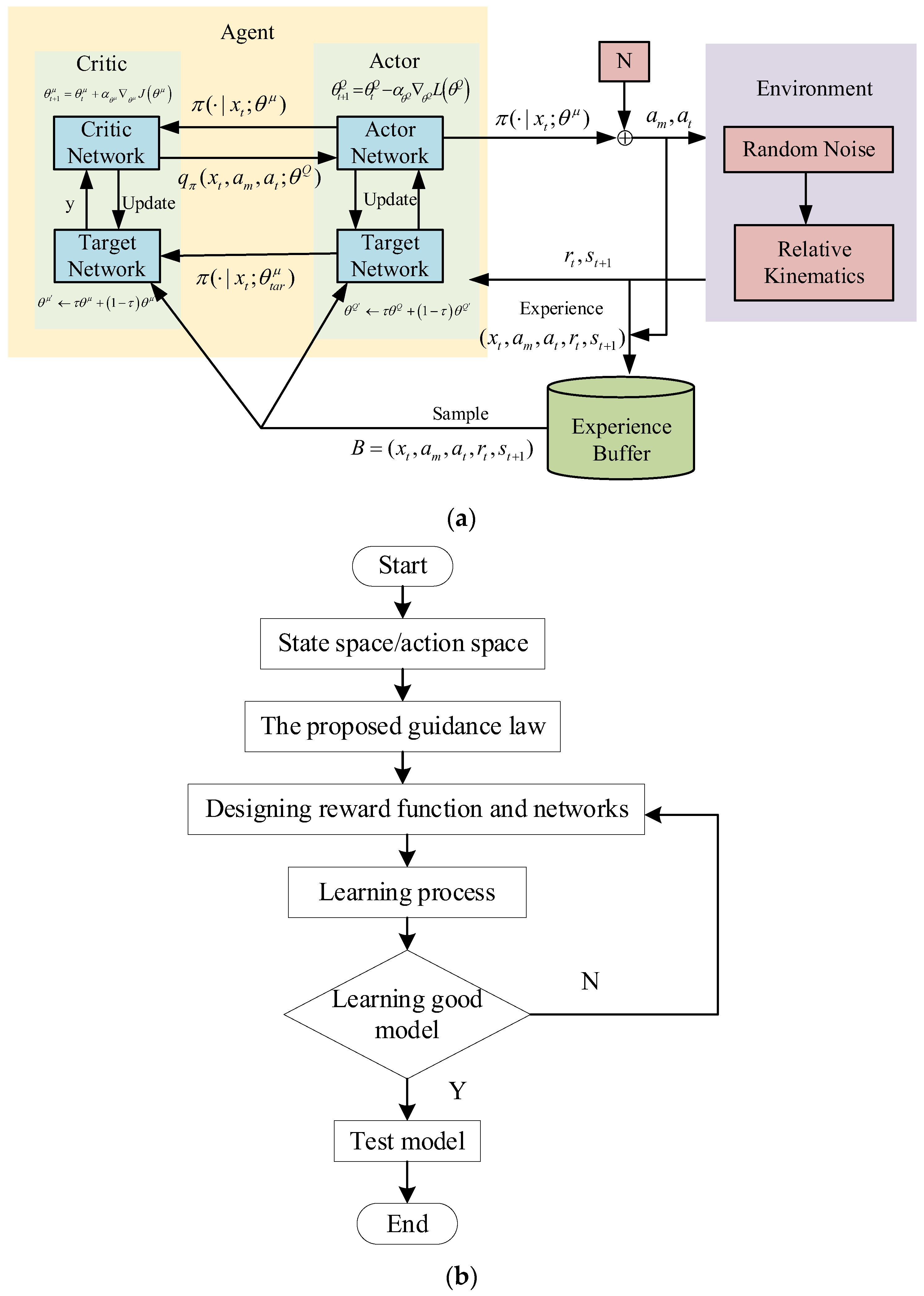
Based on the above section, we formulate the zero-sum differential Markov game problem in the DRL framework. The proposed IDGGL strategy can be learned by using the proposed algorithm. The basic structure of the system and algorithm flowchart are illustrated in Figure 2, which describes the specific implementation process. Next, the pursuit–evasion environment, states, action spaces, and the reward function are presented. Importantly, the reward function design is one of the key points.

A.

State Spaces

In the pursuit–evasion game scenario, the relative kinematic models of the pursuer and the evader are considered as state spaces, which can be designed as follows:

$$s_t=\left(r_d,\theta ,{\dot{r}}_d,\dot{\theta }\right)$$

(41)

The relative distance and the rate of the relative distance can directly reflect the success or failure of interception. The active radar seeker can provide information on the relative distance and LOS. Traditional control techniques like PNG assume that the LOS rate is known. By referring to the principle of PNG, the LOS and LOS rate are chosen as state spaces, which reflect the angle information and can ensure that the pursuer approaches the evader as parallel as possible. Thus, all states can be calculated and fully characterize the engagement states.

B.

Action Spaces

In the zero-sum differential Markov game, we consider two action spaces in the continuous space, which are the normal accelerations of the pursuer and the evader $a=(a_m,a_t)$.

$$a_m\in \left({-n}_{M}g,n_{M}g\right)$$

(42)

$$a_t\in \left({-n}_{T}g,n_{T}g\right)$$

(43)

where $n_M$ and $n_T$ denote the limit coefficients of the acceleration. It can be seen that the accelerations of the two agents are limited to a certain range, which is beneficial for the control command.

C.

Reward Function

In order to successfully intercept the evader, a reasonable reward function not only affects the learning speed and feasibility but also reflects the interception efficiency of the pursuer. Therefore, a proper reward function design is crucial for learning the optimal interception guidance law. According to the pursuit–evasion information, the reward function is designed as follows.

(1) The terminal reward $r_e$. This term reflects whether the pursuer successfully intercepts the evader or not. This function is designed as

$$\begin{array}{c}{r}_e=\left\{\begin{array}{cc}{a}_1& r_d<r_D\\ -1& r_d>r_D\end{array}\right.\end{array}$$

(44)

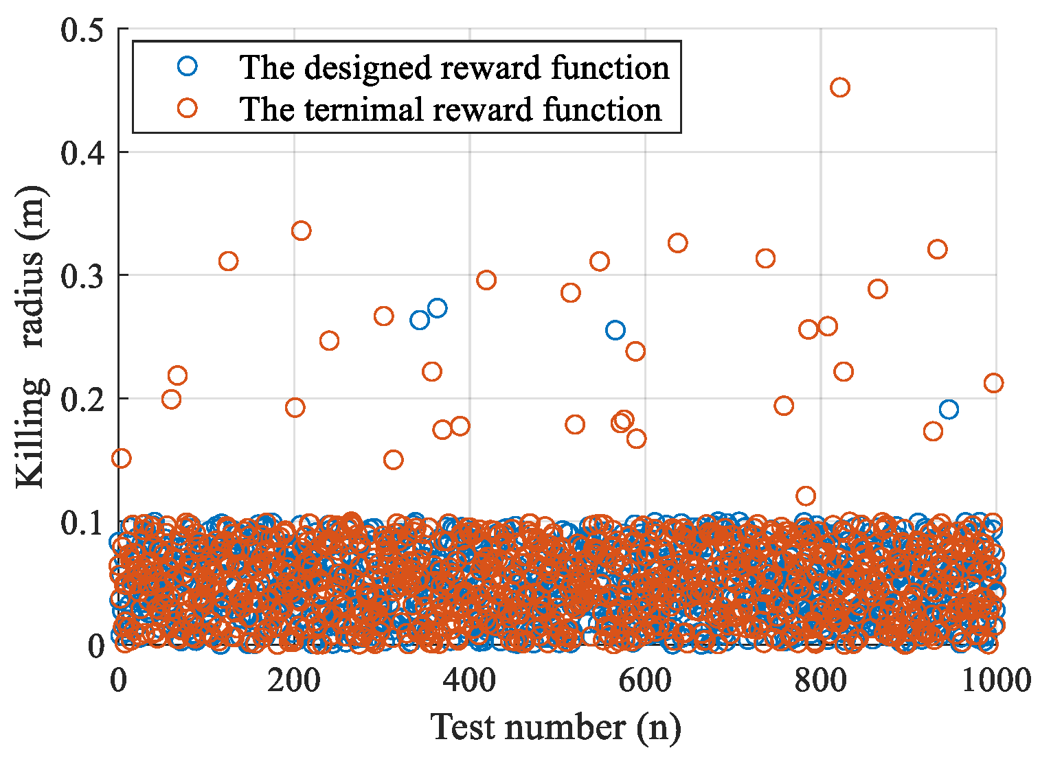
where $r_D$ represents the distance of successful interception. In most cases, $r_D$ is also the interception radius, which is set as $r_D=$ 0.1 m. $a_1$ is the interception reward.

(2) The relative distance reward $r_z$. This term means that the pursuer tried to intercept the evader. The closer the pursuer is to the evader, the higher the reward that will be obtained. This function is designed as

$$\begin{array}{c}{r}_z=-k_r{\left(\frac{r_d}{r_0}\right)}^2\end{array}$$

(45)

where $r_0$ is the initial relative distance between the pursuer and the evader; $k_r$ is a constant weight.

(3) The control effect reward $r_a$. This term takes into account the overload of the pursuer and encourages the pursuer to intercept the evader within the minimum energy consumption. This function is designed as

$$\begin{array}{c}{r}_a={-k}_a{\left(\frac{a_m}{a_{mmax}}\right)}^2\end{array}$$

(46)

where $a_{mmax}$ is the limited overload of the pursuer; $k_a$ is a constant weight.

(4) The LOS reward $r_v$. This term refers to proportional navigation guidance (PNG), which ensures that the pursuer intercepts the evader as close as possible in parallel. This term also ensures that the evader is maintained within the pursuer’s LOS. The function is designed as

$$\begin{array}{c}{r}_v=-k_{v1}{\left(\frac{\theta }{{\theta }_0}\right)}^2-k_{v2}{\left(\frac{\dot{\theta }}{{\dot{\theta }}_0}\right)}^2\end{array}$$

(47)

where ${\theta }_0$ is the initial LOS, ${\dot{\theta }}_0$ denotes the initial rate of the LOS, and $k_{v1}$ and $k_{v2}$ are constant weights.

In summary, the total designed reward function is

$$\begin{array}{c}r\left(s_i,a_{mi},a_{ti}\right)=r_e+r_p=r_e+(r_z+r_a+r_v)\end{array}$$

(48)

where $r\left(s_i,a_{mi},a_{ti}\right)$ is the reward function in Equation (16). $r_e$ is the terminal reward. $r_p$ is the process reward.

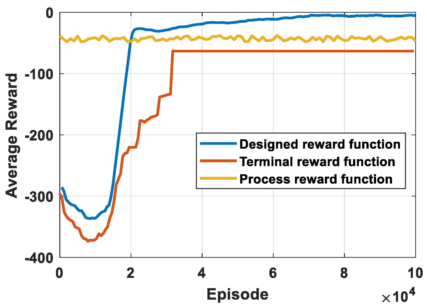
The proposed reward function is a comprehensive function, which consists of interception accuracy, energy consumption, and interception distance.

Remark 4.

Since the process of DRL is stochastic in nature, the selected parameters of the reward function are not quantitative. In this paper, based on a lot of training results, the parameters of the reward function are selected as shown in

Table 1. The parameters of the reward function.

Parameters	${\mathit{a}}_1$	${\mathit{k}}_{\mathit{r}}$	${\mathit{k}}_{\mathit{a}}$	${\mathit{k}}_{\mathit{v}1}$	${\mathit{k}}_{\mathit{v}2}$
value	100	10	0.5	0.1	0.1

.

In order to improve the training efficiency, the normalized tips are adopted in the training process. The normalized states and actions are defined as follows:

$${\overline{r}}_d=\frac{r_d}{r_0},\overline{\theta }=\frac{\theta }{{\theta }_0},{\overline{\dot{r}}}_d=\frac{{\dot{r}}_d}{{\dot{r}}_0},\overline{\dot{\theta }}=\frac{\dot{\theta }}{{\dot{\theta }}_0},{\overline{a}}_m=\frac{a_m}{a_{mmax}},{\overline{a}}_t=\frac{a_t}{a_{tmax}}$$

where ${\left(·\right)}_0$ represents the initial value of the variable $\left(·\right)$, and $a_{max}$ stands for the maximum acceleration of two agents.

D.

Neural Network Structure and Hyperparameter Setting

Inspired by the DDPG algorithm, the actor–critic NN is shown in Figure 3. Both networks have a similar structure, which is composed of four-layer fully connected neural networks. The input layer of the actor network (Figure 3a) is states; the output layer of the actor network is actions. The input layer of the critic network (Figure 3b) is states and actions; the output layer of the critic network is Q-value. Two hidden layers are considered, which are activated by the Relu function. The numbers of two hidden layers are set as 128 and 64, respectively. The ReLU function is defined as follows:

$$\begin{array}{c}ReLU\left(x\right)=\left\{\begin{array}{c}xx\ge 0\\ 0x<0\end{array}\right.\end{array}$$

(49)

The output layer is activated by the Tanh function, which can be expressed as

$$\begin{array}{c}Tanh\left(x\right)=\frac{e^x-e^{-x}}{e^x+e^{-x}}\end{array}$$

(50)

From Equation (48), it can be seen that the output layer is limited in (−1,1). Therefore, the problem of action saturation can be avoided.

The details of the input layer, hidden layers, and output layer are shown in

Table 2. The architecture of the actor–critic network.

Layer	Actor Network		Critic Network
	Units	Activation Function	Units	Activation Function
Input	4 (states)	None	5 (states + actions)	None
Hidden layer 1	64	ReLU	64	ReLU
Hidden layer 2	16	ReLU	16	ReLU
Output	1	Tanh	1	Tanh

. All hyperparameters are listed in

Table 3. Hyperparameters setting.

Parameters	Values
Maximum steps	1000
Maximum episodes	1000
Actor learning rate	0.0005
Critic learning rate	0.0005
Experience buffer	5000
Minibatch samples	128
Discount factor	0.99
Soft update coefficient	0.1
Gradient steps	−1
Action noise	0.1
Mean attraction constant	0.05
Sampling time	0.01
Policy	Mlp-policy

.

4. Simulation Results and Analysis

In the training process, to ensure diversity in random samples, we select several random positions, random flight angles, random LOS angles, and random accelerations. The details are given in

Table 4. Random initial condition of training process.

Parameters	Maximum	Minimum
$x_M$	0 m	100 m
$y_M$	0 m	100 m
$x_T$	400 m	500 m
$y_T$	0 m	100 m
${\gamma }_M$	0°	160°
${\gamma }_T$	120°	10°
LOS	5°	−5°
${\tau }_M,{\tau }_T$	0.1 s	0.2 s
$n_M,n_T$	10	0

. The speeds of the pursuer and evader are V_M = 120 m/s and V_T = 100 m/s, respectively. The simulation occurs during the terminal guidance phase. Additionally, the acceleration is limited to a reasonable range. The simulation scenario can refer to reference [22]. The experiment environments are tested on the PC platform with i7-9750H CPU @ 2.90 GHZ, 32 G DDR3, using Python (Python 3.7) and PyTorch (PyTorch 12.1).

4.1. Training Results

First, before training the RL model, we use an experience dataset to test the correctness of the simulation environment. In this experiment, the initial states of the pursuer and the evader are random. The results are presented in Figure 4 and

Table 5. The Monte Carlo result of the training process.

Successful	Fail	Monte Carlo Number
478	522	1000

.

Figure 4 shows the 50 interception processes where the pursuer and the evader are untrained, where the pursuer’s acceleration is random in $a_m\in \left({-n}_{M}g,n_{M}g\right)$. It can be seen that the pursuer may fail to intercept the evader. To further illustrate this result, 1000 Monte Carlo tests are presented in Table 5. It can be found that the pursuer can successfully intercept the evader with 52.2% accuracy. Figure 4 and Table 5 show the training data, which are samples and untrained data. The results of Figure 4 and Table 5 reveal the correctness of the RL simulator.

Then, according to the above parameter setting, the training process is learned to test the proposed IDGGL strategy. The results are shown in Figure 5.

To make the results compact, the average reward and average steps of each episode are presented together in Figure 5a. The left y-coordinate represents the average reward, and the right y-coordinate represents the average steps. It can be noted that the average reward (blue line) of the proposed IDGGL can converge within 20,000 episodes. It can be seen that the average steps (orange line) of the proposed algorithm can converge around 60 steps, which means that the pursuer can intercept the evader within 65 steps. Figure 5b presents the interception distance of the learning process. It can be observed that the average interception distance can converge to a reasonable interception region. All results illustrate the effectiveness of the proposed IDGGL.

To further demonstrate the better performance of the designed reward function (Equation (46)), we designed a comparative experiment. In this experiment, we compared the terminal reward function, the process reward function, and the designed reward function for the learning process. The results are shown in Figure 6.

The comparison results of the average reward are shown in Figure 6. It can be found that the average reward of the designed reward function will converge within 20,000 episodes, while the average reward of the terminal reward function will converge within 37,000 episodes. Additionally, the average reward of the designed reward function is larger than the average reward of the terminal reward function. Both results illustrate that the design reward function has a faster training speed and better reward. The reason behind this observation is that the pursuer cannot learn the full information and may stay in certain positions. Furthermore, it can be found that only in the process reward function, the training process may not converge. The reason is that the pursuer does not know if the interception is successful or not.

4.2. Test Results

In the test experiment, to verify the effectiveness of the proposed IDGGL algorithm, four experiments are conducted.

4.2.1. The Effectiveness of the Proposed IDGGL and the Designed Reward Function

First, the learned model is used to prove the effectiveness of the proposed IDGGL. In this experiment, the pursuer adopts the trained model to intercept the evader. The results are shown in Figure 7.

Figure 7 shows the interception process of 50 games’ trained data between pursuers and evaders, where the pursuer’s acceleration is chosen by the trained model. It can be seen that the pursuer almost successfully intercepts the evader. This result reveals the effectiveness of the proposed IDGGL. Additionally, by comparing Figure 4 and Figure 7, it can be seen that the proposed algorithm can train a better interception model.

To further validate the effectiveness of the designed reward function, two reward functions are compared in 1000 Monte Carlo tests. A total of 1000 Monte Carlo results with random initialization conditions are presented in Figure 8 and

Table 6. The details of the Monte Carlo results.

Reward Function	Successful	Fail	Monte Carlo Number
The designed reward function	992	8	1000
The terminal reward function	948	52	1000

.

Figure 8 shows 1000 Monte Carlo results with random initialization conditions for the designed reward function and the terminal reward function. It can be found that the pursuer almost successfully intercepts the evader with different reward functions. From Table 6, it can be found that the pursuer can successfully intercept the evader with 99.2% accuracy by the designed reward function.

4.2.2. Intercepting a Game Evader

In this experiment, the game process of the pursuer and the evader is test, where the pursuer adopts the proposed IDGGL, while the evader performs the corresponding optimal escape strategy. The initial positions of the pursuer and the evader are set at (0 m, 0 m) and (500 m, 0 m), respectively. Their initial flight path angles are α = 40° and β = 120°, respectively. The initial LOS is 0°. The interception results are presented in Figure 9.

Figure 9a shows the trajectory of the pursuer and the evader. It is a game process where the pursuer and the evader are unwilling to lose their own interests. Thus, the interception paths appear to be straight. The change in the relative distances of two agents is presented in Figure 9b. It can be clearly noted that both results indicate that the pursuer can intercept the evader successfully. Figure 9c,d show the performance curves of the closing speed and the LOS rate. Figure 9c reveals that the closing speed converges to zero, which implies that the pursuer intercepts the evader as soon as possible. Figure 9d presents that the LOS rate is maintained at zero, which implies that the pursuer intercepts the evader with a parallel manner. It also keeps up with the interception characteristics of PNG. This result indicates that the motion direction of the pursuer and the target remains unchanged, and the paths appear to be straight. The acceleration curves of two agents are presented in Figure 9e, which reveals that the proposed guidance algorithm provides smooth guidance command within the limited acceleration range. It can be seen from Figure 9e that the accelerations of the pursuer and the evader approach the maximum amplitude within 0.1 s. Therefore, it can be concluded that the evader tries its best to escape from the pursuer, while the pursuer tries its best to intercept the evader, which reflects that the game process is an accelerated interception process.

4.2.3. Intercepting Maneuvering Evaders

To further demonstrate the general applicability of the proposed IDGGL, two different maneuvering manners of the evader are considered. In case 1, the evader executes a square-wave maneuver with a magnitude of $10g$, as shown:

$$a_t=100\mathrm{s}\mathrm{g}\mathrm{n}\left(\sin \left(2\mathrm{t}+\mathsf{\pi }/2\right)\right)$$

In case 2, the evader performs a sin-wave maneuver with a magnitude of $10g$, as shown:

$$a_t=100\mathrm{s}\mathrm{i}\mathrm{n}(2t+\mathsf{\pi }/2)$$

The simulation results for this experiment are shown in Figure 10.

Figure 10a,b present the flight trajectories of the two agents and the change in the relative distance between two agents under different conditions. It can be seen that the proposed IDGGL can successfully intercept the evader with different maneuvering manners. Additionally, the relative distance between the two agents tends to zero, which also reveals that the evader is intercepted by the pursuer. Figure 10c,d show the acceleration of two agents within $10g$. It can be seen that the proposed IDGGL can provide a smooth acceleration command for the pursuer within $10g$.

4.2.4. Comparison for Different Guidance Laws

To further demonstrate the advantage of the proposed guidance law, the OGL and DGGL are compared with the proposed IDGGL, respectively. The simulation environment’s three methods are the same, which means that the information of the target’s motion $(\dot{r},\dot{\theta })$ is known in the three methods. We define the control effort as $J=\underset{0}{\overset{\infty }{\int }}{u}^T\left(\tau \right)u\left(\tau \right)d\tau$. It can quantify the advantages of the proposed IDGGL. The evader executes a sin-wave maneuver. The compared results are shown in Figure 11 and

Table 7. The performance summary of the three guidance laws.

Methods	Control Effort (J)	Simulation Time (s)	Monte Carlo Number
OGL	289.4	1.647	100
DGGL	264.2	0.883	100
Our method	152.4	0.058	100

.

Figure 11a indicates the trajectories of three different guidance laws. It can be seen that all guidance laws can successfully intercept the evader. Traditional control commands (OGL, DG) require manual parameter settings, most of which are based on expert experience. The parameters of the proposed method are learned by DRL. Therefore, the parameters are optimal, and the proposed method can save simulation time. Figure 11b presents the accelerations of the pursuer with three guidance laws. It can be concluded that the smallest acceleration amplitude is our algorithm, the second is the OGL, and the largest is the DGGL. More important, the acceleration of the DGGL may exceed 10g, which is harmful to the system. Figure 11c shows the control effort of the pursuer. Table 7 summarizes the average result obtained from 100 Monte Carlo simulations. It can be noted that the control effort of our proposed method is the least compared with the other two guidance laws, which implies that our proposed guidance law saves energy consumption and is more intelligent. Moreover, the simulation time of the three guidance laws were compared. It can be found that the simulation time of our proposed method is the shortest. All in all, by comparing the three methods, it can reflect the advantages of the proposed method in terms of the interception accuracy, interception time, and cost energy of the pursuer. The proposed IDGGL algorithm can intercept evaders with a fast time and a lower control effort.

5. Conclusions

This paper proposes an intelligent differential game guidance law based on DRL. First, the interception problem is converted into finding the Nash equilibrium strategy. We proposed an algorithm for obtaining the optimal IDGGL strategy. Subsequently, a reasonable reward function, which includes the interception accuracy, the energy consumption, and the interception distance, is designed for the engagement. The simulation results demonstrate that the proposed IDGGL algorithm exhibits superior performance in terms of acceleration response, control efforts, and quick computation. Moreover, compared with traditional guidance laws, the IDGGL algorithm can confront the complex game environment and avoid tedious manual setting. Additionally, compared to other reinforcement learning guidance laws, the proposed IDGGL algorithm takes into account the effect of the evader. Importantly, by designing a more reasonable reward function, the proposed IDGGL algorithm has good performance in intercepting different maneuvering evaders. The intercepting accuracy is up to 99.2%. All in all, simulation experiments demonstrate the efficiency of the proposed IDGGL. However, the limitations and challenges of the proposed approach include the following: the escape strategies of the evader, real-time processing constraints, the impact of obstacles, complex scenarios. By using a state observer, employing advanced hardware, and using optimizing algorithms, the specific limitations can be solved. In the terminal guidance phase, when the pursuer and the evader reach a certain height, the proposed intelligent differential game guidance law can be used in practical applications. For implementing the proposed method in real-world systems, some modifications should be considered, which include adjustments for environmental variability, integration with existing systems, and considerations for robustness and reliability. For example, when the pursuer and evader are in a 2D scenario and the environmental state is known, the algorithm proposed can completely achieve the interception of the evader. In future work, more complex scenarios should be considered, such as changes in heading angle and the interceptor’s altitude, which would enhance the robustness and applicability of our guidance laws. Additionally, the impact of external disturbances should be considered, such as winds, which lead to the development of more resilient guidance laws capable of operating under various environmental conditions.