Article

Beyond Static Obstacles: Integrating Kalman Filter with Reinforcement Learning for Drone Navigation

by
Francesco Marino
*,† and
Giorgio Guglieri
Dipartimento di Ingegneria Meccanica e Aerospaziale (DIMEAS), Politecnico di Torino, 10129 Torino, Italy
*
Author to whom correspondence should be addressed.
These authors contributed equally to this work.
Aerospace 2024, 11(5), 395; https://doi.org/10.3390/aerospace11050395
Submission received: 28 March 2024 / Revised: 6 May 2024 / Accepted: 14 May 2024 / Published: 15 May 2024

Abstract

:
Autonomous drones offer immense potential in dynamic environments, but their navigation systems often struggle with moving obstacles. This paper presents a novel approach for drone trajectory planning in such scenarios, combining the Interactive Multiple Model (IMM) Kalman filter with Proximal Policy Optimization (PPO) reinforcement learning (RL). The IMM Kalman filter addresses state estimation challenges by modeling the potential motion patterns of moving objects. This enables accurate prediction of future object positions, even in uncertain environments. The PPO reinforcement learning algorithm then leverages these predictions to optimize the drone’s real-time trajectory. Additionally, the capability of PPO to work with continuous action spaces makes it ideal for the smooth control adjustments required for safe navigation. Our simulation results demonstrate the effectiveness of this combined approach. The drone successfully navigates complex dynamic environments, achieving collision avoidance and goal-oriented behavior. This work highlights the potential of integrating advanced state estimation and reinforcement learning techniques to enhance autonomous drone capabilities in unpredictable settings.

1. Introduction

Autonomous drones hold immense potential across various industries, with applications ranging from surveillance to delivery [1]. However, their effective operation in dynamic environments poses significant challenges. Traditional path-planning methods, often designed for static settings, can become inadequate when objects and conditions change unpredictably. Accurate state estimation of moving elements and adaptive path-planning techniques are essential to tackle this.
State estimation involves determining objects’ positions and potentially other characteristics (e.g., velocities) in the relevant environment. This information is crucial for decision making of path planning but becomes complex when objects are in motion.
Traditionally, researchers have gravitated towards model-based control methods like model predictive control (MPC), which capitalizes on known system dynamics and optimization techniques for structured control. While MPC is proficient at leveraging precise models for prediction and control, its effectiveness is hampered by the dual challenges of requiring highly accurate models and undertaking computationally intensive online trajectory optimization. In contrast, reinforcement learning (RL) excels at deriving complex control policies directly from data, adapting to environmental changes and uncertainties without needing explicit models.
Our approach combines RL’s adaptive learning capabilities with the Kalman filter’s strength in estimating states in uncertain environments. We propose using a set of IMM Kalman filters to estimate and predict the positions of target waypoints, in our context defined as the centers of gates. The Kalman filter supports real-time trajectory planning by forecasting waypoint locations over variable time horizons. Subsequently, the Proximal Policy Optimization (PPO) reinforcement learning (RL) algorithm uses the new enriched observation space for optimal path planning in dynamic environments. RL enables drones to learn through trial and error, maximizing rewards for desired behaviors like goal-reaching and obstacle avoidance.
This hybrid methodology not only overcomes the limitations posed by reliance on accurate models and computational bottlenecks but also enhances the agility of drones by enabling more responsive and adaptive control strategies in real-time, unpredictable scenarios. Additionally, in line with established robotics practices, our framework treats navigation and perception as distinct problems. This decoupling offers several advantages. Perception focuses on interpreting raw sensor data (such as images or lidar scans) to identify objects and build an understanding of the environment. Conversely, navigation leverages this perceived information to plan paths, control movement, and avoid obstacles. By treating these as separate modules, we can develop specialized algorithms for each task. This enhances modularity, allowing us to upgrade perception systems with better sensors or algorithms without overhauling the navigation components. This facilitates isolated testing and refinement of individual modules, leading to a more robust overall solution.
The schema reported in Figure 1 presents a novel approach for autonomous drone navigation in dynamic environments. Our contribution includes successfully demonstrating the Interactive Multiple Model (IMM) Kalman filter for accurate gate position prediction over varying time horizons, enabling improved optimal path planning, success rate, and convergence of the Proximal Policy Optimization (PPO) in a dynamic environment. Our results analysis validates the proposed framework, demonstrating the drone’s ability to successfully navigate complex scenarios while achieving collision avoidance and goal-oriented behavior.

Related Works

Policy search is a crucial aspect of reinforcement learning, focusing on identifying the optimal parametric policy that maximizes the expected return from sampled trajectories [2,3]. This process is instrumental in effectively discovering how to generate actions to achieve desired outcomes in various scenarios. Policy search methods diverge into two main categories based on their approach to exploring stochastic trajectories: step-based and episode-based methods [2,4].
Step-based methods introduce exploration noise at each control time step within the action space, aiding in the stepwise generation of trajectories. These methods [5,6,7,8,9] are especially prevalent in tasks requiring continuous control. They have been successfully applied in diverse areas, such as enabling legged robots to learn agile motor skills [10] and managing the control of a simulated race car to navigate at the edge of its friction limits [11]. The advantage of step-based algorithms lies in their ability to develop end-to-end black-box control policies, facilitating a direct mapping from observations to control commands.
In contrast, episode-based policy search strategies [4,12,13,14] incorporate exploration noise directly into the policy’s parameter space, but only at the start of each episode. These methods excel in crafting movement primitives [15,16,17,18], which serve as succinct parameterizations of a robot’s control policy. A notable example within this category is the task-parameterized dynamic motor primitives (DMPs) [15], offering compact policy frameworks that are highly adaptable. By fine-tuning the parameters of these models, robots can rapidly acquire new skills and tackle complex control challenges across various activities, including baseball [19], ball in the cup [20], and table tennis [21]. Episode-based approaches are particularly practical in encapsulating complex skill representations that would otherwise be challenging for human experts to model directly.
Proximal Policy Optimization (PPO) is primarily an episode-based policy search method. PPO optimizes a policy by maximizing an objective function that compares the new policy to an old policy, ensuring that the update is not too large, which helps maintain stable training. While it operates over episodes, gathering experience over multiple steps to update the policy, the distinctive aspect of PPO and similar policy optimization methods is their focus on adjusting the policy parameters in a manner that improves performance over entire episodes of interaction with the environment, rather than optimizing the policy at every single time step based on immediate feedback.
Proximal Policy Optimization (PPO) algorithms, despite offering advantages in stability and ease of implementation, exhibit limitations related to the observation space. PPO’s performance may degrade in real-world, non-static environments characterized by significant shifts in the observation space. When faced with unanticipated observations, the algorithm’s reliance on consistent state distributions between training and deployment phases can lead to policy failures [22,23,24]. This sensitivity highlights the need for frequent retraining or advanced observation strategies to enhance robustness in dynamic settings.
Our preferred strategy enhances the algorithm’s robustness through advanced observation strategies. This technique prepares the algorithm for a wide range of possible observations, reducing the likelihood of encountering completely unfamiliar situations. By integrating these advanced observation strategies, the goal is to develop a PPO algorithm that maintains its performance advantages while being capable of handling the complexities and unpredictability of real-world environments.

2. Methodology

2.1. Simulation Environment

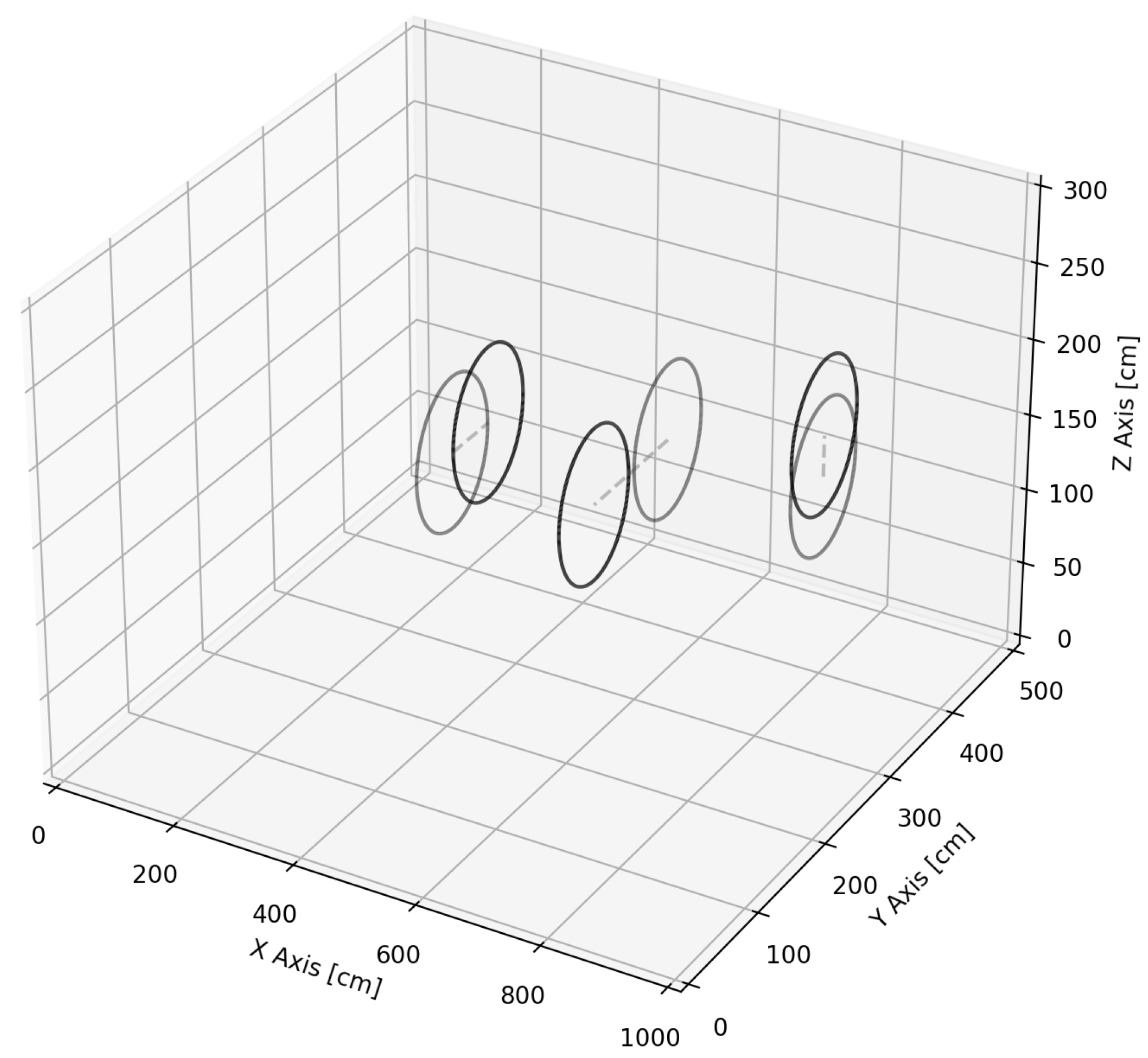
Our research has led to the development of a unique simulation framework explicitly tailored for drone path planning (Figure 1). The framework leverages the constructor provided by OpenGym [25] to support the possibility of using this environment with multiple reinforcement learning (RL) algorithms. This custom-designed environment, built upon Python, offers a solution that significantly lowers computational demands while perfectly fitting our specialized requirements. Unlike AirSim, which requires high-performance system resources due to its computational intensity, our environment is optimized for both efficiency and task relevance (Figure 2).
Our simulation environment is a three-dimensional drone navigation simulator intricately designed from the ground up to allow for extensive customization [26]. It encapsulates a drone navigation game, where the primary objective is maneuvering through a series of gates, thereby challenging the drone’s path-planning and navigation capabilities. This environment is structured within a class that sets several critical parameters essential for the simulation’s dynamics, including the drone’s starting position, the initial locations of the gates, and the simulation space’s spatial dimensions, quantified by width, height, and length (Table 1).
The framework introduces distinct scenarios [27], each designed within a continuous state-action space, providing a variety of challenges that affect both the drone and the gates’ behaviors. This tailored approach bridges the gap in existing simulation options and enhances the precision and adaptability of drone path-planning algorithms by offering a more realistic and flexible testing ground. It is possible to evaluate, for each time step, the validity of the action taken by the agent to avoid shortcuts or non-realistic solutions to the challenges we are interested in. An overview of how the simulation environment changes state is reported in the section as part of Algorithm 1.
At the heart of our simulation’s flexibility and adaptability lies the precise definition of the action space, which is crucial for implementing effective drone path-planning algorithms. The action space, denoted as A, is formalized within the simulation framework as follows:
A = a R 3 1 a i 1 , for i { x , y , z }
where a = ( a x , a y , a z ) represents the vector of actions corresponding to the drone’s velocity components along the x, y, and z axes, respectively. This continuous, bounded three-dimensional action space enables the drone to execute a wide range of movements, facilitating the exploration of diverse flight paths and maneuvers within the simulated environment. Each action component a i is multiplied by the drone’s maximum translational speed per axis, transforming the sampled action into a realistic velocity value. This multiplication not only allows for any continuous value of translational speed within the specified limits but also allows further parameterization of the simulation. Furthermore, the notation + 1 and 1 within the action vector explicitly identifies the direction of the movement along the respective axes, with + 1 indicating movement in the positive direction of the axis and 1 indicating movement in the negative direction. By allowing for the specification of speeds within a carefully defined range and incorporating directional control, our environment ensures that the drone’s actions remain within realistic boundaries, thus promoting the development of practical, efficient, and adaptable path-planning strategies. Integrating such a mathematically and physically coherent action space within our simulation framework enriches the realism of the drone navigation challenges. It significantly enhances the applicability and effectiveness of the RL algorithms employed.
v = a v max
where:
  • v represents the resulting velocity vector of the drone in R 3 ;
  • a = ( a x , a y , a z ) is the action vector sampled from the action space A;
  • ⊙ denotes the element-wise multiplication (Hadamard product);
  • v max = ( v max , x , v max , y , v max , z ) is the vector of maximum translational speeds for each axis;
  • 1 a i 1 for i { x , y , z } , where + 1 and 1 in a identify the direction of movement along the respective axes, with + 1 indicating movement in the positive direction of the axis and 1 indicating movement in the negative direction.
Algorithm 1 Overview of the Algorithm that Operates the Environment
1:
Input:  r ( s , a ) , S , C o n f i g u r a t i o n = { }
2:
Initial setting of the environment
3:
while Not done with episodes do
4:
    Call Reset method
5:
    Randomly reset the coordinates of the gates: Y gates , Z gates
6:
    Initialize the observation space for the episode: s 0 ρ ( S )
7:
    Initialize the data collection for the episode: ( s 0 , a 0 , r 0 )
8:
    Call Step method
9:
    while Not done with episode do
10:
        Collect of the observation space, action and reward: ( s i , a i , r i )
11:
        Check for collision or invalid actions
12:
        if Collisions or Terminate = True then Call Reset method
13:
        end if
14:
        Collect additional logs
15:
    end while
16:
    Update PPO Policy: Δ θ = arg max θ E min r t ( θ ) A ^ t , clip r t ( θ ) , 1 ϵ , 1 + ϵ A ^ t
17:
end while
18:
Output: Agent model and logs saved.
Finally, the framework developed has two critical checks implemented to ensure the drone (agent) navigates successfully within the simulation parameters: boundary adherence and gate passage verification.
The first check, is_inside_boundaries, ensures the drone remains within the predefined environmental limits. It evaluates if the drone’s current position, given by its x, y, and z coordinates, does not exceed the environment’s maximum dimensions of the environment assigned for a specific episode. This safeguard is essential for maintaining the simulation’s integrity, preventing the drone from navigating outside the virtual space designed for testing.
The second check, is_inside_gate, is designed to assess whether the drone successfully navigates through a designated gate, a critical component of the navigation challenge. This function identifies currently active gates and their positions. Gates are modeled as cylinders, and the drone’s position relative to a gate’s axis and dimensions determines whether it has successfully passed through. The function calculates the drone’s distance to the gate’s axis and compares this with the gate’s radius to ascertain passage. Furthermore, it considers the drone’s altitude in relation to the gate’s height and position, offering a comprehensive check that accounts for the three-dimensional nature of the challenge.
Furthermore, it is important to note that the framework does not include a direct check for flight mechanic feasibility, which is crucial for ensuring that the drone’s trajectories are theoretically possible and practically executable. To address this, we have introduced a trajectory analysis module. This module evaluates the smoothness of the drone’s path [28]. It eliminates solutions that, despite being theoretically valid, would not be feasible in a real-world scenario due to the drone’s physical limitations and flight dynamics. This enhancement aims to bridge the gap between simulation and real-world applicability, ensuring that the trajectories generated within our simulation are optimized for computational efficiency and aligned with the drone’s flight capabilities.
Together, these functions form an essential part of the simulation environment, guiding the simulation’s dynamics by ensuring that the drone operates within set boundaries and successfully interacts with the gates as expected. Through these checks, the environment offers a structured yet flexible platform for evaluating drone navigation algorithms under realistic conditions.

2.2. Proximal Policy Optimization (PPO)

This section aims to demystify the core components of PPO, providing clear definitions and explanations of its fundamental concepts and mathematical formulations. Moreover, our research emphasizes the observation space’s significant yet often understated role in shaping the performance of RL algorithms. Changes to the observation space can profoundly impact the policy’s behavior, learning efficiency, and, ultimately, the agent’s success in achieving its goals. By modifying the observation space, researchers can better tailor the learning process to suit specific environments or tasks, opening new avenues for optimizing and applying PPO in diverse domains. Thus, alongside clarifying the algorithm’s terminology, this section highlights the influence of the observation space on PPO’s functionality and the innovative potential within our work. This focus enriches the reader’s comprehension of PPO and sets the stage for presenting our contributions to advancing its application through observation space adjustments.
Proximal Policy Optimization (PPO) [22] represents a notable advancement in reinforcement learning, introducing a surrogate objective function that enables multiple gradient steps using the same minibatch of experiences. This approach contrasts with conventional on-policy strategies like Advantage Actor–Critic (A2C) [29], which require discarding experience samples after a single optimization step. The surrogate objective function of PPO assesses the new and old policies through a likelihood ratio, aiming to maximize the expected return while ensuring policy updates remain within a predefined trust region.
A key feature of PPO is its clipped objective function, which is designed to regulate the magnitude of policy updates. This mechanism prevents substantial changes after each optimization step, promoting cautious and incremental updates. Such a strategy mitigates the risk of performance degradation—a common issue in on-policy gradient methods. Traditional policy gradient approaches are known for their sensitivity to minor parameter space adjustments, which can significantly affect performance. This discrepancy necessitates using small learning rates in policy gradient methods to manage high variance. Clipped PPO addresses these challenges by constraining the objective function, ensuring that policy modifications are within specific limits during training.
Furthermore, clipping can be extended to the value function, adopting a similar principle: constraining changes in the parameter space to ensure that variations in Q-values remain controlled and within a designated threshold. Consequently, this method guarantees a stable evolution in the targeted metrics, irrespective of the smoothness of changes in the parameter space.
The Proximal Policy Optimization (PPO) optimizes a policy function, π θ ( a | s ) , parameterized by θ , which defines the probability of selecting action a given state s. The algorithm aims to adjust θ to maximize expected returns from the environment, which are calculated based on the rewards received for each action taken in a given state.
PPO introduces a novel approach to policy optimization by utilizing a clipped objective function, ensuring smooth updates and preventing drastic policy changes. The updated policy parameters, θ n e w , are obtained by optimizing the following objective function:
θ n e w = arg max θ L C L I P ( θ ) ,
with L C L I P ( θ ) defined as
L C L I P ( θ ) = E ^ t min ( r t ( θ ) A ^ t , clip ( r t ( θ ) , 1 ϵ , 1 + ϵ ) A ^ t ) .
In this equation, r t ( θ ) = π θ ( a t | s t ) π θ o l d ( a t | s t ) represents the probability ratio of the new to the old policy for taking action a t in state s t . The term A ^ t is the advantage estimate at time t, and ϵ is a small positive hyperparameter defining the clipping range. clip ( r t ( θ ) , 1 ϵ , 1 + ϵ ) : This clipping function limits the value of r t ( θ ) to the range [ 1 ϵ , 1 + ϵ ] . The parameter ϵ is a hyperparameter that controls the degree to which the new policy can diverge from the old policy. This clipping prevents overly large policy updates that could lead to instability in the training process; finally, min ( · , · ) is the minimum between the unclipped and clipped objective. This ensures that the objective does not benefit from changes to the probability ratio that would move it outside of the interval defined by [ 1 ϵ , 1 + ϵ ] , thereby encouraging updates that improve the policy while maintaining a degree of similarity to the old policy.
The advantage function, A ^ t = Q t V θ ( s t ) , is crucial for guiding the policy update direction and magnitude. It calculates the relative benefit of taking action a t in state s t , with Q t as the expected return and V θ ( s t ) as the expected return under the policy π θ for state s t . The advantage function is intrinsically linked to both reward and PPO optimization. More specifically, the reward function expected return, Q t , is a function of the accumulated rewards defined by the environment’s reward function. PPO also leverages A ^ t to update the policy π θ . A positive A ^ t encourages the policy to increase the probability of a t , while a negative A ^ t discourages it.
The observation space plays a critical role in the formulation of PPO, as it influences the calculation of π θ ( a | s ) , V θ ( s t ) , and consequently, A ^ t . Modifications to the observation space can significantly impact the algorithm’s ability to accurately estimate these values, thereby affecting the overall performance and effectiveness of the policy optimization process. The observation space determines the information available to the agent, influencing the scope of its decision making. The reward function then identifies what the agent should strive for within that observable environment. Through continuous feedback, the agent learns to prioritize observations that lead to higher rewards, shaping its actions to maximize long-term gains. In this specific work, the reward function uses the drone’s newly acquired pose and the gate’s position to assess the value of the action taken. In this work, IMM predictions form a crucial component of the observation space. The reward function does not directly utilize the accuracy of IMM predictions in relation to the observed gate position. Nevertheless, better alignment between the prediction and the true gate location at the crossing time leads to a higher reward due to more actions being positively evaluated. Moreover, accurate IMM predictions enable faster, smoother navigation toward the gate, increasing the overall reward due to the temporal component of the reward function. Additionally, improved IMM predictions help the drone maintain proximity to the desired trajectory, further contributing to a higher reward. PPO can operate in discrete and continuous action spaces, employing neural networks representing the policy and value functions. These networks output probabilities for discrete action spaces or parameters for probability distributions in continuous spaces.
To encourage exploration and mitigate premature convergence to suboptimal policies, PPO incorporates an entropy bonus into its objective function:
L = L C L I P ( θ ) + c 1 L V F ( θ ) c 2 S [ π θ ] ( s ) ,
where L V F ( θ ) represents the value function loss, S [ π θ ] ( s ) the policy entropy for state s, and c 1 and c 2 are coefficients for the value function loss and entropy bonus, respectively.
The training process, with the parameters reported in Table 2, in PPO alternates between sampling data through environment interaction under the current policy and optimizing the clipped objective function with respect to θ . This iterative process, involving multiple minibatch update epochs, incrementally refines the policy parameters to achieve better performance.

2.3. Reward Function

The reward function plays a crucial role in guiding the learning process of the agent. It essentially shapes the agent’s behavior by providing positive feedback for desirable actions and negative feedback for undesirable ones. The reward function comprises several components designed to encourage specific aspects of the agent’s behavior. A Gate Reward is awarded when the agent successfully navigates through a gate, promoting goal-oriented navigation. For encouraging efficient pathfinding, a Forward Movement Reward is given when the agent moves forward towards the nearest gate, calculated via the dot product of the movement vector and the gate vector. Completing the entire course is highly incentivized with a Game Completion Reward. Conversely, the function imposes a Collision Penalty for colliding with objects and a Time Penalty per time step, adjusted by the number of gates passed plus one, to discourage delays and inefficient paths. These components collectively guide the agent towards achieving the task efficiently and effectively, underlining the reward function’s importance in the PPO algorithm.
R = A g · G c + M · G f + C · G c o m p + T · P c + P t · N g
where:
  • G c = 25.0 is the reward for passing through an active gate.
  • G f = 0.5 is the reward for moving towards the nearest gate in the forward direction.
  • G c o m p = 100.0 is awarded upon completing the course, i.e., passing all gates.
  • P c = 100.0 is the penalty for colliding with obstacles.
  • P t = 0.65 is the time penalty applied at each time step, scaled by N g , the count of gates passed plus one.
  • A g indicates whether an active gate was passed (1 if true, 0 otherwise).
  • M is the condition for forward movement reward (1 if the movement vector aligns with the gate vector and the distance to the center of the gate is appropriate, 0 otherwise).
  • T indicates whether the agent has collided (1 if true, 0 otherwise).
  • C indicates whether all gates have been passed (1 if true, 0 otherwise).
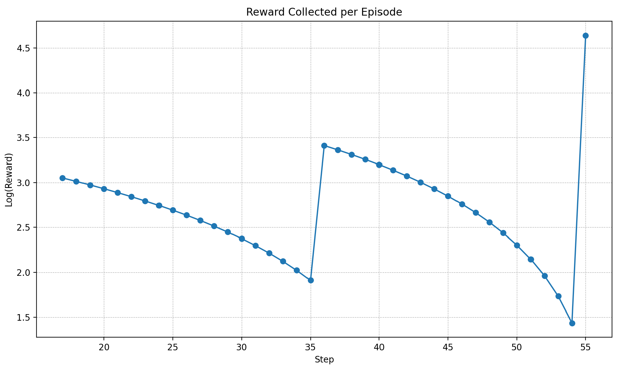
This formulation strategically integrates incentives for goal-directed behavior and penalties for inefficient or incorrect actions, guiding the agent’s learning in complex environments (Figure 3).

2.4. IMM Kalman and Representation of the Enriched Observation Space

In the context of reinforcement learning, specifically within Proximal Policy Optimization (PPO), the composition of the observation space is critical for enabling the agent to make informed decisions. This paper outlines a cohesive approach to integrating the IMM Kalman filter predictions into the observation space of a PPO framework, thereby enhancing the decision-making process. The Interactive Multiple Model (IMM) Kalman filter represents an advancement in state estimation for systems exhibiting multiple dynamic behaviors. The following discussion assumes familiarity with the basic principles of Kalman filtering, focusing on how the IMM Kalman was used to enrich the observation space of the RL simulation. Its foundational aspects and mathematical underpinnings are thoroughly documented in references [30,31,32,33,34,35,36].
We define the following components of the observation space in our PPO framework:
  • Agent Pose ( p a g e n t ) : The coordinates and orientation of the agent for self-localization.
  • Active Gate Pose ( p g a t e ) : The position and orientation of the tracked gate, which the agent aims to navigate through.
  • Nearest Gate Distance ( d g a t e ) : The spatial distance between the agent and the nearest gate, guiding the agent towards its goal.
  • Average Agent Speed ( v a g e n t ) : Reflects the agent’s movement speed, crucial for planning and trajectory estimation.
  • Gate Velocity ( v g a t e ) : Important for anticipating the motion of dynamic gates or targets.
The IMM Kalman filter enhances these observations by providing robust predictions of future gate positions, even in the presence of noise and maneuvers. This allows the agent to plan more effectively and achieve higher levels of navigation performance.
IMM efficiently combines the strengths of multiple Kalman filters, where each model M i that predicts the state x ^ i ( k ) and covariance P i ( k ) is tailored to a specific dynamic behavior, thereby accommodating the non-linearities and mode switches that may occur in complex systems. The IMM algorithm operates by computing a set of mode probabilities that reflect the likelihood of each model being the correct representation of the system’s current state. These probabilities are updated based on the observed data and the prediction performance of each filter, resulting in a combined output that optimally predicts the gate’s future position p ^ g a t e ( t + Δ t ) .
M = { M 1 , M 2 , , M n }
These models account for various motion dynamics, such as constant velocity and acceleration. The critical components of the IMM Kalman filter include the mixing process, model-specific filtering, and model probability update, encapsulated by the following steps:
  • Mixing Process: At the beginning of each time step, the state estimate and covariance from the previous step are mixed across the models based on the model probabilities, preparing a set of initial conditions for each filter.
  • Model-Specific Filtering: A Kalman filter prediction and update cycle is executed using the mixed initial conditions for each model. This results in updated state estimates and covariances for each model.
  • Model Probability Update: The likelihood of each observation given the model-specific predictions is calculated; it is then used to update the probabilities of each model being the correct representation of the system dynamics.
  • Combination: Finally, all models’ state estimates and covariances are combined based on the updated model probabilities to produce the overall state estimate and covariance.
In order to tailor the IMM Kalman filters to the problem, two distinct dynamic models were employed. The first model prioritized stability by assuming a constant velocity motion profile for the gate. Its state-space representation is as follows:
x ( k + 1 ) = F 1 x ( k ) + w ( k )
where x ( k ) = [ y , z , v y , v z ] T , and w ( k ) represents the process noise so that the position components of the state vector are updated with the following prediction equations:
y ( k + 1 ) = y ( k ) + Δ t · v y ( k )
z ( k + 1 ) = z ( k ) + Δ t · v z ( k )
The second model, designed for responsiveness, incorporated a constant acceleration assumption:
x ( k + 1 ) = F 2 x ( k ) + w ( k )
with x ( k ) = [ y , z , v y , v z , a y , a z ] T , so that the prediction equations for the position components in this model are
y ( k + 1 ) = y ( k ) + Δ t · v y ( k ) + Δ t 2 2 · a y ( k )
z ( k + 1 ) = z ( k ) + Δ t · v z ( k ) + Δ t 2 2 · a z ( k )
The IMM filter’s probabilistic framework switches between the two filter models (F1 and F2) based on the availability of relevant information. A transition probability matrix, denoted by P , governs the likelihood of transitioning from one model to another at each time step. This allows the filter to adapt to changing target dynamics. For instance, if the gate exhibits a sudden change in velocity, the filter might transition from F 1 (constant velocity) to F 2 (constant acceleration) to better capture this behavior. The transition probability matrix between models is given below:
P = p 11 p 12 p 21 p 22
where:
  • p i j represents the probability of transitioning from model M i at time step k to model M j at time step k + 1 .
  • Common choices for the diagonal elements ( p 11 and p 22 ) are values close to 1 (e.g., 0.9 or 0.95) to promote filter stability and persistence.
  • The off-diagonal elements ( p 12 and p 21 ) represent the probability of switching to the other model. These values can be tuned based on the target’s expected frequency of maneuvers.
More specifically, in the case of the use case presented in this manuscript, we design a transition probability matrix with the following values:
P = 0.925 0.075 0.075 0.925
This configuration favors staying in the current model most of the time but allows for switching to the other model when necessary, i.e., when the target changes direction. The specific values chosen for the transition probabilities depend on your application and the dynamics of the target you are tracking.
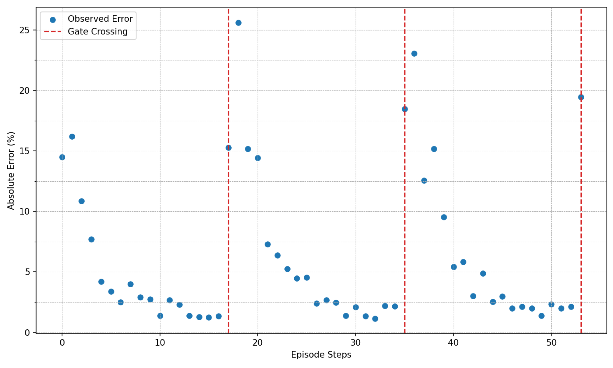
The methodology employed to enhance the observation space of the agent, reported schematically as part of Algorithm 2, by the Interactive Multiple Model (IMM) Kalman filter enables seamless adaptation to systems with multiple operational modes or when the system dynamics are not precisely known in advance. This adaptability is crucial for maintaining accuracy in operating environments that vary significantly. This behavior is exemplified in Figure 4, which shows the observation of absolute error between the simulated position of the simulated and the estimated position by the Kalman filter of the center of the gate for a specific episode. Notably, the filter requires some observations (approximately six) before it can predict the position of the relevant gate at the next crossing time with an acceptable error margin of less than 5 percent. This initial inaccuracy is attributed to a deliberately poor initialization of parameters intended to test the method’s ability to adjust. Moreover, at each gate crossing, the target gate is dynamically relocated to the next one, necessitating a reset in the filter. This reset forces the filter to adapt to the new dynamics, demonstrating its ability to adjust to changing conditions swiftly.
Algorithm 2 IMM Kalman Filter Integration for Gate Position Prediction
1:
Input: Current observation space including agent’s pose p agent , active gate’s pose p gate , nearest gate distance d nearest , agent’s average speed v agent , and gate’s velocity v gate .
2:
Output: Updated observation space with predicted future gate pose p gate , t .
3:
procedure EstimateTimeToGate( d nearest , v agent )
4:
     t to gate d nearest v agent
5:
    return  round ( t to gate )
6:
end procedure
7:
procedure IMMKalmanFilterPrediction
8:
    Initialize model probabilities, transition probabilities, and model set
9:
    for Each model in the IMM set do
10:
        Predict the gate’s position using the Kalman filter prediction step
11:
        Calculate the likelihood of the observation given the predicted state
12:
    end for
13:
    Update model probabilities based on observations
14:
    Combine model predictions based on updated probabilities
15:
    return combined prediction and estimation of the gate position at crossing time as p gate , t c r o s s i n g
16:
end procedure
17:
procedureUpdateObservationSpace
18:
     t to gate EstimateTimeToGate( d nearest , v agent )
19:
     p gate , t
20:
     p gate , t c r o s s i n g  IMMKalmanFilterPrediction
21:
end procedure
22:
UpdateObservationSpace
The ability to quickly adjust to new operational modes and unpredicted changes in system dynamics is key to achieving high levels of autonomy. It ensures that the system remains resilient in the face of uncertainty, minimizing the impact of errors and enhancing its overall performance. By effectively dealing with dynamic changes and uncertainties, the IMM Kalman filter significantly contributes to the robustness and reliability of autonomous systems, enabling them to operate efficiently in complex and ever-changing environments.
To formalize the implementation, let the enhanced observation vector at time step ( t ) be represented as p gate ( t + Δ t ) , or p gate , t in short, which includes the components presented in the beginning of the paragraph along with the IMM Kalman filter predictions:
s ( t ) = p agent , p gate , d nearest , v agent , v gate , p ^ gate ( t + Δ t ) T
By incorporating IMM Kalman filter predictions into the PPO observation space, we significantly enhance the agent’s ability to anticipate future environmental states, facilitating more effective decision making and planning. This integrated approach underscores the importance of sophisticated state estimation techniques in developing intelligent, adaptable reinforcement learning agents.
Finally, within this work we use the term pose specifically to refer to the spatial coordinates and orientation of both the drone and the gates. Algorithm 2 operates under the assumption that the drone knows the current position of the closest gate at each time step. While we do not explicitly model target occlusion, the Kalman filter’s inherent robustness allows it to manage short-term occlusions by treating them as potential outliers.

3. Experiments and Results

In our research, we design our experiments to assess the proposed framework’s validity. We employ three main criteria to evaluate the performance of the PPO, elaborated as follows:
  • Cumulative Reward: This metric measures the agent’s performance in its assigned task, where superior scores indicate optimized actions towards fulfilling the objective. This metric was beneficial during the tuning phase of the PPO algorithm when comparing two different parametrizations of the same model. It cannot be used to categorize the performances across episodes.
    R total = t = 1 T r t
    where:
    • R total represents the total cumulative reward obtained by the agent throughout an episode.
    • t is the time step within the episode, ranging from 1 to T.
    • T denotes the terminal time step of the episode at which the episode ends.
    • r t is the reward received at time step t, reflecting the immediate benefit of the action taken by the agent at that step.
  • Average Reward per Action: Measures the quality of decisions, with higher values indicating superior decision making, leading to higher rewards for each action.
    Average Reward per Action = Total Reward in an Episode Total Actions in an Episode
  • Success Rate: Represents the ratio of episodes where the agent accomplishes its objective, indicating the reliability of a model trained. This metric is also used to analyze the test environments.
    Success Rate = Number of Successful Episodes Total Episodes
Given the metrics described above, we guide the development and assessment of the framework by dividing the results according to the performances in the two matrices: success rate and average reward per action.
  • High average reward and high success rate indicate optimal algorithm performance.
  • Low average reward but high success rate suggest frequent goal accomplishment with room for proficiency improvement.
  • High average reward but low success rate implies proficient actions but less frequent goal accomplishment.
  • Low average reward and low success rate indicate subpar algorithm performance.
These metrics comprehensively evaluate the effectiveness and efficiency of reinforcement learning algorithms under study. Additionally, the matrices average reward per action and success rate can be calculated to compare the framework presented with other approaches objectively. The results of the metrics described above and the nominal conditions used are reported in Table 3.

3.1. Flying through Dynamic Gates

Facing the daunting challenges of generating realistic simulation environments for autonomous navigation and defining training strategies for high-speed obstacle avoidance and precision navigation through narrow gates, our study embarked on an innovative approach. We crafted custom environments within a simulation framework, populating them with gates moving according to various simulated patterns. At the core of our solution is the sophisticated trajectory planning generated by the agent, coupled with the adaptive observation space produced by the IMM Kalman filter. Our policies underwent rigorous evaluation, demonstrating remarkable adaptability and robustness across unseen simulated environments, thereby addressing the initial challenges and propelling our methodology beyond existing paradigms for autonomous drone navigation.
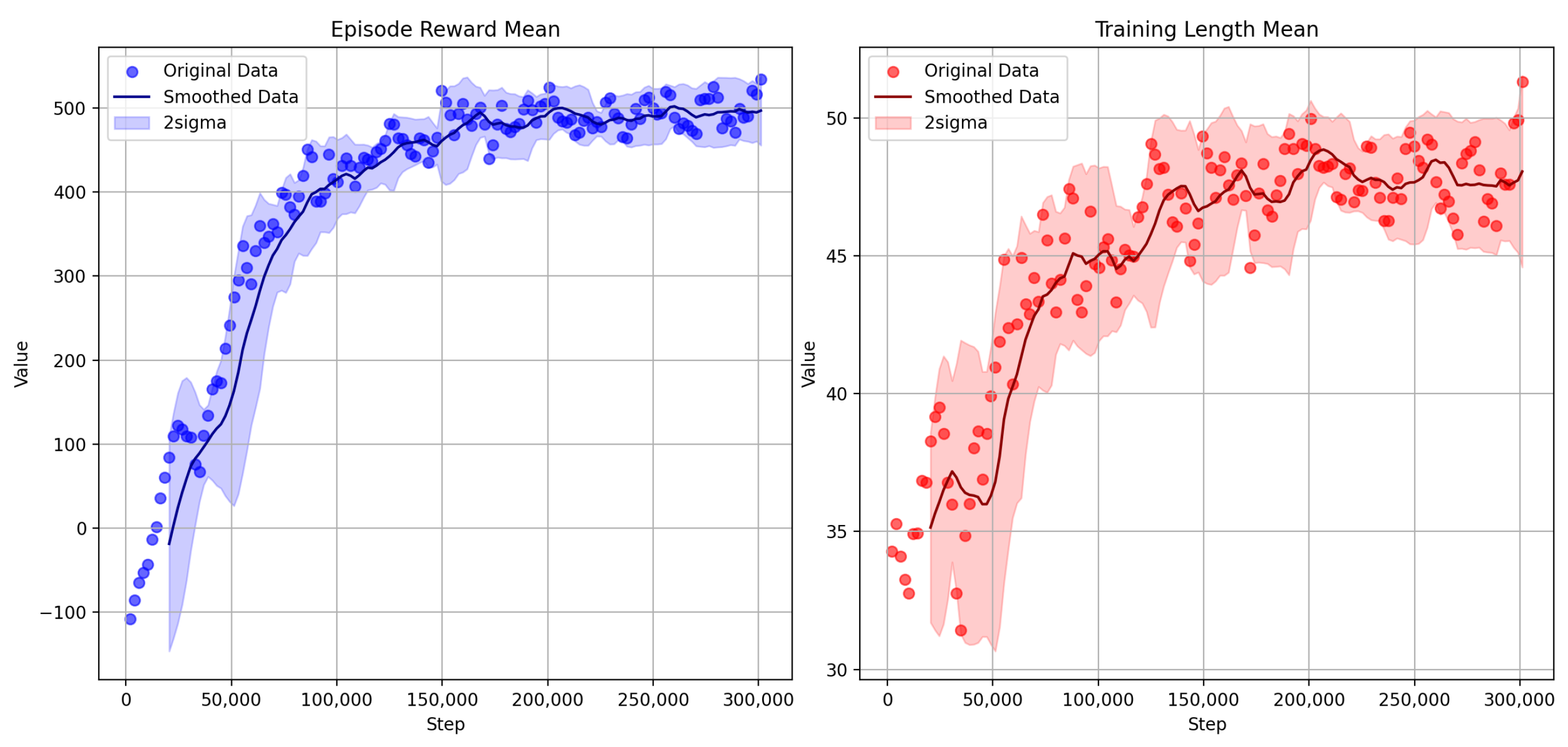
The strategic creation of custom environments within the OpenAI Gym framework facilitated rapid iterations of training and evaluation, which is critical for swift improvements in reward systems and observation space definition. The training process, executed over 300,000 steps—equivalent to approximately 6000 training episodes (Figure 5)—produced a model capable of generating actions that effectively respond to environmental challenges. Following the training, we designed a rigorous testing protocol to assess policy performance under various conditions, ensuring effectiveness beyond controlled simulation settings. The test environments, fixed configurations distinct from the training phase, (Figure 6) challenged the agent with unforeseen obstacles and scenarios, verifying the policies’ generalizability and ability to apply learned strategies in new contexts. The policies’ successful navigation and obstacle avoidance demonstrate their efficacy, validating the training and development process and highlighting their significant potential for practical autonomous navigation tasks.
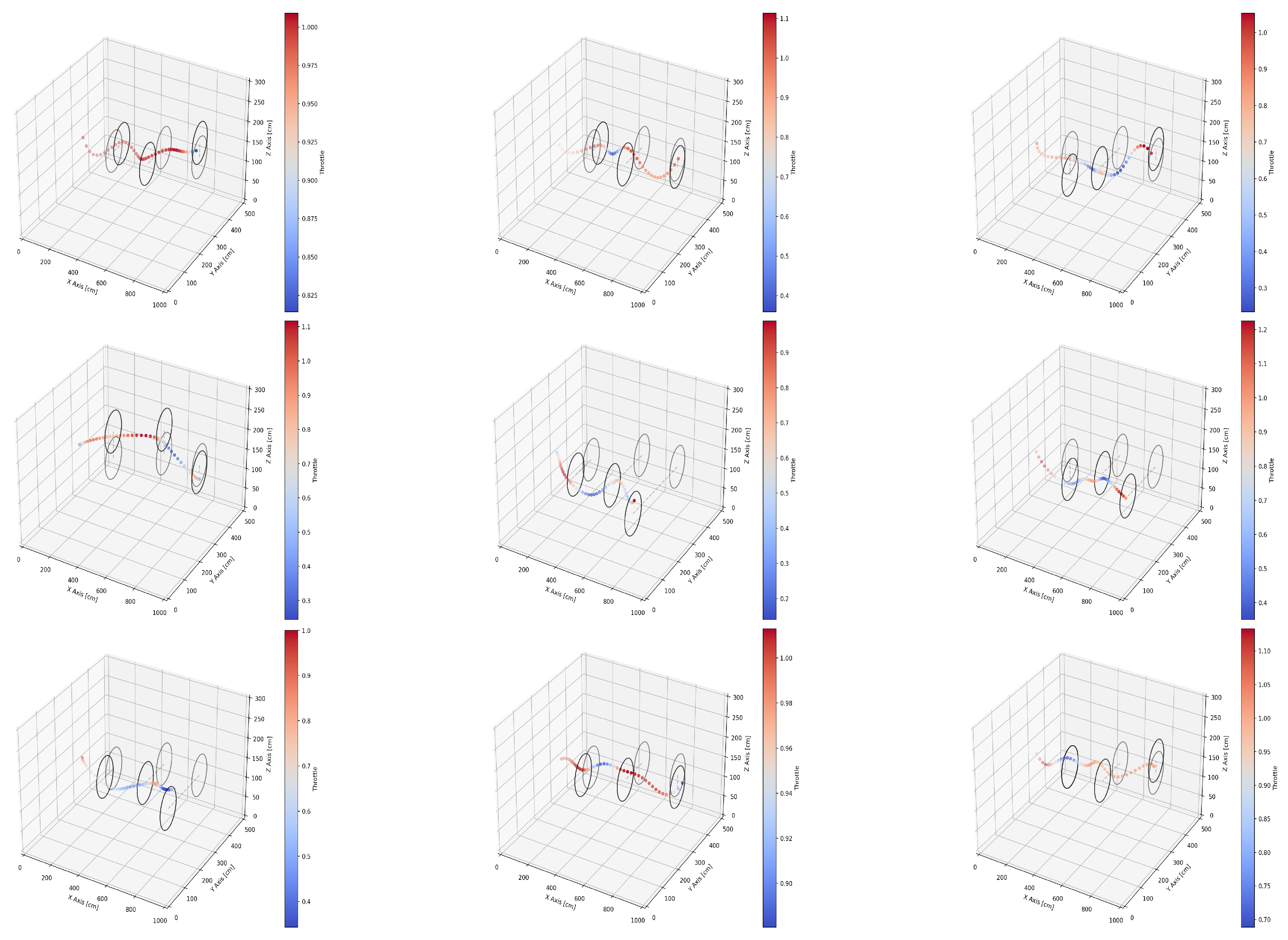
As part of our testing protocol, we evaluated the agent’s trajectory across various training episodes for a given model candidate. This analysis provided insights into progressive performance optimization, particularly in navigating through gates at increasing speeds. With each additional training step, the trajectory became more refined, improving both precision and velocity. Initially, the agent’s movements were tentative and indirect, reflecting a cautious approach to navigating through gates. However, training progression saw a marked shift towards efficiency and speed, with the agent adopting more direct paths and demonstrating a clear increase in confidence. This evolution highlights the effectiveness of our training regimen, not just in enabling the agent to learn and adapt over time but also in optimizing its path for faster completion times, incentivized by the reward function. The visualized trajectories in Figure 7 illustrate the agent’s development from a cautious navigator to a proficient and swift operator, underscoring the value of continuous learning and adaptation in achieving optimal performance.
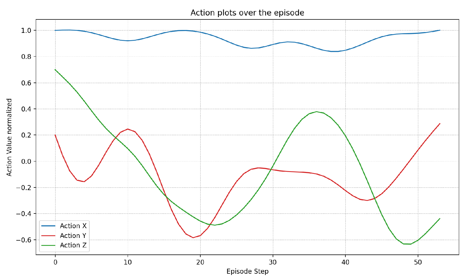
Furthermore, we provided a detailed view of the drone’s control strategy as it navigated through episodes by investigating the action values across the episode steps for the X (blue), Y (green), and Z (red) axes. These plots are crucial for understanding the drone’s control dynamics, illustrating the strategic adjustments made for successful navigation. A refinement in control strategy, as evidenced by fewer extremes in the action values, suggests optimized efficiency and safety. By examining the changes in action values across training episodes, we identified areas for further optimization and refinement. As depicted in Figure 8, these action plots offer a window into the drone’s decision-making process, providing a visual interpretation of its capability to execute complex trajectories with increasing confidence and precision.

3.2. Effect of the Drone and Gate Speed

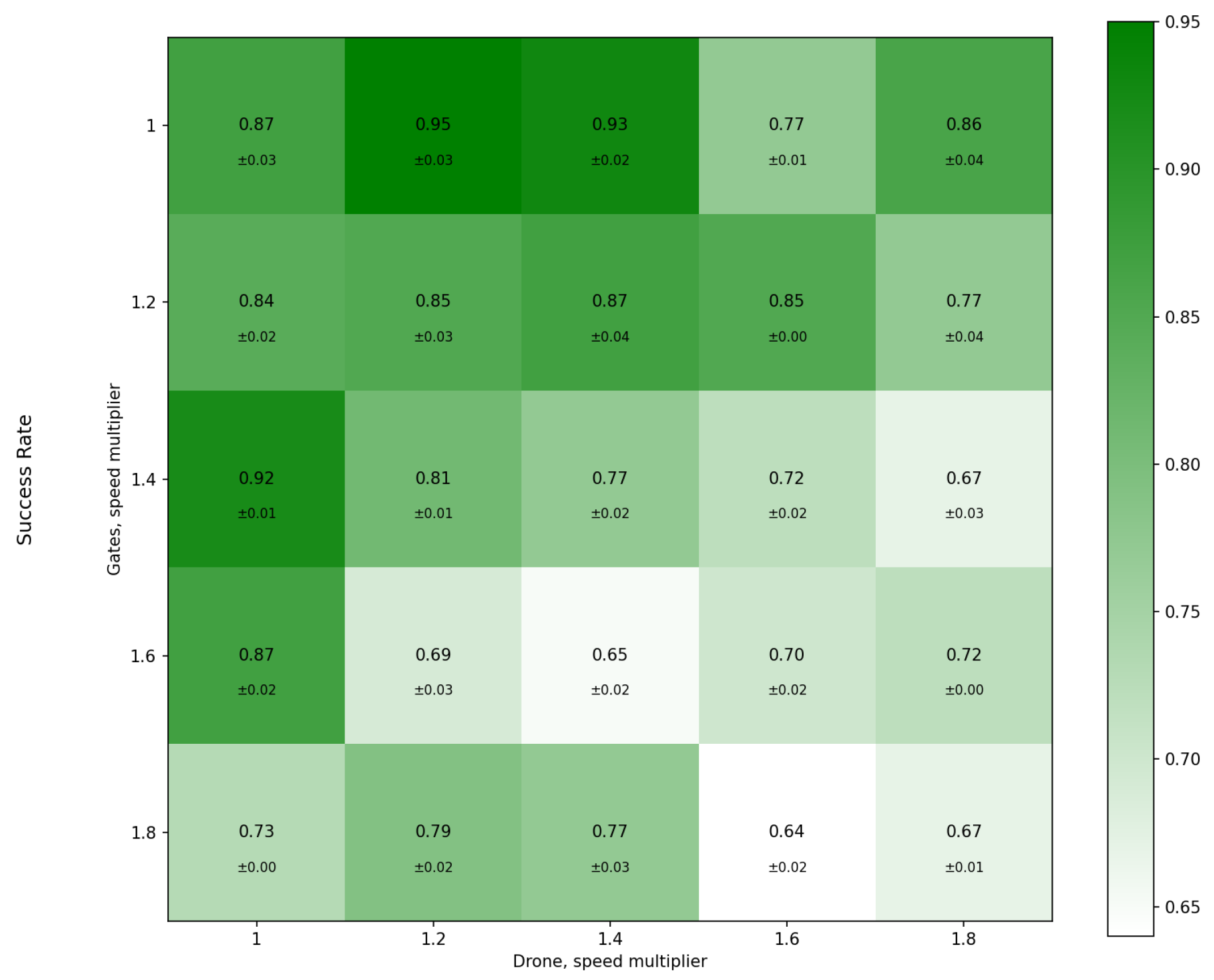
The accompanying heatmap illustrates the intricate relationship between the observation space and the autonomous drone navigation system’s performance (Figure 9). This visualization underscores the observation space’s pivotal role in facilitating the drone’s adaptability and decision-making precision, especially under varying speed conditions for both the drone and the gates. By examining the heatmap, we can observe how different combinations of speed multipliers, represented along the x-axis for the drone and the y-axis for the gates, impact the system’s success rates, with the darker green shades symbolizing higher efficacy in navigation. Notably, success rates and their respective standard deviations within each cell provide a nuanced understanding of the system’s robustness. Higher speed multipliers correspond to a diverse range of success outcomes, highlighting the system’s ability to maintain high performance across a spectrum of dynamic conditions. This demonstrates the critical importance of a well-structured observation space in enhancing the drone’s capability to navigate through moving gates. The heatmap, therefore, not only illustrates the direct impact of speed variations on performance but also reinforces the value of a comprehensive observation space in ensuring the adaptability and resilience of autonomous navigation systems.

4. Discussion and Conclusions

This study has presented a novel approach to autonomous drone navigation in dynamic environments, combining the strengths of Proximal Policy Optimization (PPO) with the Interactive Multiple Model (IMM) Kalman filter for enhanced state estimation and adaptive path planning. Our methodology demonstrates significant advancements in autonomous drones, specifically in navigating through dynamically moving gates with high precision and efficiency. The integration of IMM Kalman filters has proven particularly effective in predicting gate positions, enabling the drone to make informed decisions well in advance of approaching an obstacle. With its robust performance in complex environments, the PPO algorithm has been optimized through our unique reward function and adaptive observation space, showcasing the potential for real-world applications where dynamic obstacle avoidance is critical.
Our approach distinguishes itself from existing methods by addressing the limitations of traditional model-based control techniques and static path-planning algorithms. Unlike model predictive control (MPC), which relies heavily on accurate models and suffers from computational intensity, our RL-based framework adapts to environmental changes without requiring explicit dynamics modeling. This adaptability offers a significant advantage in scenarios where prior knowledge of the environment is limited or conditions can change unpredictably. By enriching the observation space with predicted future states, our drones can anticipate changes and adjust their path accordingly, a particularly beneficial feature in dynamic environments. Our experiments’ results underline our proposed framework’s effectiveness in enhancing autonomous drones’ agility and decision-making capabilities. By successfully navigating through moving gates with high success rates and optimized paths, we have demonstrated the practicality of our approach in scenarios similar to real-world applications, such as search and rescue operations, surveillance, and delivery services in urban environments. Looking forward, testing our framework in real-world environments will be essential to validate its applicability outside simulation settings, where we envision incorporating cameras for frame-by-frame gate detection or the use of external tracking systems, depending on the specific application scenario. Rigorous testing in real-world environments with dynamic obstacles is crucial, emphasizing edge-case analysis and uncertainty quantification to establish trust in decision making. Failure mode analysis will ensure system resilience, especially in the context of perception of the environment. Additionally, it is imperative to work within airspace regulations and focus on explainability to bolster transparency for users and regulatory bodies.
In conclusion, this study provides a compelling framework for the hybrid PPO and IMM Kalman filter approach. Our methodology overcomes traditional control methods’ computational and modeling challenges and opens new possibilities for deploying autonomous drones in dynamically changing environments. The advancements demonstrated in this work hold significant potential for a wide range of applications, marking a step forward in the quest for fully autonomous, highly adaptive unmanned aerial vehicles.

Author Contributions

Conceptualization, F.M. and G.G.; methodology, F.M.; software, F.M.; validation, F.M.; formal analysis, F.M.; investigation, F.M.; resources, F.M. and G.G.; data curation, F.M.; writing—original draft preparation, F.M.; writing—review and editing, F.M. and G.G.; visualization, F.M.; supervision, G.G. All authors have read and agreed to the published version of the manuscript.

Funding

This research received no external funding.

Data Availability Statement

The data presented in this study are available upon reasonable request from the corresponding author.

Acknowledgments

We would like to extend our sincere gratitude to Afshin Zeinaddini Meymand for his initial contribution to the research on this topic.

Conflicts of Interest

The authors declare no conflicts of interest.

References

  1. Otto, A.A.; Agatz, N.; Campbell, J.J.; Golden, B.B.; Pesch, E.E. Optimization Approaches for Civil Applications of Unmanned Aerial Vehicles (UAVs) or Aerial Drones. Networks 2018, 72, 411–458. [Google Scholar] [CrossRef]
  2. Sutton, R.S.; Barto, A.G. Reinforcement Learning: An Introduction; MIT Press: Cambridge, MA, USA, 2018. [Google Scholar]
  3. Glasius, R.; Komoda, A.; Gielen, S.C. Neural Network Dynamics for Path Planning and Obstacle Avoidance. Neural Netw. 1995, 8, 125–133. [Google Scholar] [CrossRef]
  4. Deisenroth, M.P.; Neumann, G.; Peters, J. A Survey on Policy Search for Robotics. Found. Trends® Robot. 2013, 2, 1–142. [Google Scholar]
  5. Schulman, J.; Levine, S.; Abbeel, P.; Jordan, M.; Moritz, P. Trust Region Policy Optimization. In Proceedings of the International Conference on Machine Learning, Lille, France, 6–11 July 2015; pp. 1889–1897. [Google Scholar]
  6. Williams, R.J. Simple Statistical Gradient-Following Algorithms for Connectionist Reinforcement Learning. Mach. Learn. 1992, 8, 229–256. [Google Scholar] [CrossRef]
  7. Kakade, S.M. A Natural Policy Gradient. Adv. Neural Inf. Process. Syst. 2001, 14, 1531–1538. [Google Scholar]
  8. Peters, J.; Muelling, K.; Altun, Y. Relative Entropy Policy Search. In Proceedings of the Twenty-Fourth National Conference on Artificial Intelligence (AAAI), Physically Grounded AI Track, Atlanta, GA, USA, 11–15 July 2010. [Google Scholar]
  9. Bry, A.; Roy, N. Rapidly-Exploring Random Belief Trees for Motion Planning Under Uncertainty. In Proceedings of the IEEE International Conference on Robotics and Automation (ICRA), Shanghai, China, 9–13 May 2011. [Google Scholar]
  10. Hwangbo, J.; Lee, J.; Dosovitskiy, A.; Bellicoso, D.; Tsounis, V.; Koltun, V.; Hutter, M. Learning Agile and Dynamic Motor Skills for Legged Robots. Sci. Robot. 2019, 4, eaau5872. [Google Scholar] [CrossRef]
  11. Song, Y.; Lin, H.; Kaufmann, E.; Duerr, P.; Scaramuzza, D. Autonomous Overtaking in Gran Turismo Sport Using Curriculum Reinforcement Learning. In Proceedings of the 2021 IEEE International Conference on Robotics and Automation (ICRA), Xi’an, China, 30 May–5 June 2021. [Google Scholar]
  12. Stulp, F.; Sigaud, O. Path Integral Policy Improvement with Covariance Matrix Adaptation. In Proceedings of the 29th International Conference on Machine Learning (ICML), Edinburgh, Scotland, 26 June–1 July 2012. [Google Scholar]
  13. Sun, Y.; Wierstra, D.; Schaul, T.; Schmidhuber, J. Efficient Natural Evolution Strategies. In Proceedings of the 11th Annual Conference on Genetic and Evolutionary Computation, Montreal, MN, Canada, 8–12 July 2009; pp. 539–546. [Google Scholar]
  14. Sehnke, F.; Osendorfer, C.; Rückstieß, T.; Graves, A.; Peters, J.; Schmidhuber, J. Policy Gradients with Parameter-Based Exploration for Control. In Proceedings of the International Conference on Artificial Neural Networks, Prague, Czech Republic, 3–6 September 2008; Springer: Berlin/Heidelberg, Germany, 2008; pp. 387–396. [Google Scholar]
  15. Schaal, S. Dynamic Movement Primitives—A Framework for Motor Control in Humans and Humanoid Robotics. In Adaptive Motion of Animals and Machines; Springer: Berlin/Heidelberg, Germany, 2006; pp. 261–280. [Google Scholar]
  16. Paraschos, A.; Daniel, C.; Peters, J.R.; Neumann, G. Probabilistic Movement Primitives. In Advances in Neural Information Processing Systems; NeurIPS Proceedings; Curran Associates, Inc.: Lake Tahoe, NV, USA, 5–10 December 2013; pp. 2616–2624. [Google Scholar]
  17. Williams, B.; Toussaint, M.; Storkey, A.J. Modelling Motion Primitives and Their Timing in Biologically Executed Movements. In Advances in Neural Information Processing Systems; NeurIPS Proceedings; Curran Associates, Inc.: Vancouver, BC, Canada, 3–6 December 2007; pp. 1609–1616. [Google Scholar]
  18. Ijspeert, A.J.; Nakanishi, J.; Hoffmann, H.; Pastor, P.; Schaal, S. Dynamical Movement Primitives: Learning Attractor Models for Motor Behaviors. Neural Comput. 2013, 25, 328–373. [Google Scholar] [CrossRef] [PubMed]
  19. Peters, J.; Schaal, S. Reinforcement Learning of Motor Skills with Policy Gradients. Neural Netw. 2008, 21, 682–697. [Google Scholar] [CrossRef]
  20. Kober, J.; Peters, J.R. Policy Search for Motor Primitives in Robotics. In Advances in Neural Information Processing Systems; NeurIPS Proceedings; Curran Associates, Inc. (Jun 2009): Vancouver, BC, Canada, 8–10 December 2008; pp. 849–856. [Google Scholar]
  21. Kober, J.; Oztop, E.; Peters, J. Reinforcement Learning to Adjust Robot Movements to New Situations. In Proceedings of the International Joint Conference on Artificial Intelligence (IJCAI), Catalonia, Spain, 16–22 July 2011. [Google Scholar]
  22. Schulman, J.; Wolski, F.; Dhariwal, P.; Radford, A.; Klimov, O. Proximal Policy Optimization Algorithms. arXiv 2017, arXiv:1707.06347. [Google Scholar]
  23. Lillicrap, T.P.; Hunt, J.J.; Pritzel, A.; Heess, N.; Erez, T.; Tassa, Y.; Silver, D.; Wierstra, D. Continuous control with deep reinforcement learning. arXiv 2019, arXiv:1509.02971. [Google Scholar]
  24. Gandhi, D.; Pinto, L.; Gupta, A. Learning to Fly by Crashing. In Proceedings of the IEEE/RSJ International Conference on Intelligent Robots and Systems (IROS), Vancouver, BC, Canada, 24–28 September 2017; pp. 3948–3955. [Google Scholar]
  25. Brockman, G.; Cheung, V.; Pettersson, L.; Schneider, J.; Schulman, J.; Tang, J.; Zaremba, W. OpenAI Gym. arXiv 2016, arXiv:1606.01540. [Google Scholar]
  26. Saeedi, S.; Thibault, C.; Trentini, M.; Li, H. 3D Mapping for Autonomous Quadrotor Aircraft. Unmanned Syst. 2017, 5, 181–196. [Google Scholar] [CrossRef]
  27. Rupprecht, C.; Laina, I.; DiPietro, R.S.; Baust, M. Learning in an Uncertain World: Representing Ambiguity through Multiple Hypotheses. In Proceedings of the International Conference on Computer Vision (ICCV), Venice, Italy, 22–29 October 2017; pp. 3611–3620. [Google Scholar]
  28. Richter, C.; Bry, A.; Roy, N. Polynomial Trajectory Planning for Aggressive Quadrotor Flight in Dense Indoor Environments. In Proceedings of the International Symposium on Robotics Research (ISRR), Venice, Italy, 22–29 October 2013. [Google Scholar]
  29. Mnih, V.; Badia, A.P.; Mirza, M.; Graves, A.; Lillicrap, T.; Harley, T.; Silver, D.; Kavukcuoglu, K. Asynchronous Methods for Deep Reinforcement Learning. In Proceedings of the International Conference on Machine Learning, New York, NY, USA, 19–24 June 2016; PMLR. pp. 1928–1937. [Google Scholar]
  30. Blom, H.A.P. An efficient filter for abruptly changing systems. In Proceedings of the 23rd IEEE Conference on Decision and Control, Las Vegas, NV, USA, 12–14 December 1984; Volume 2, pp. 656–658. [Google Scholar]
  31. Bar-Shalom, Y.; Li, X.R. Multitarget-Multisensor Tracking: Principles and Techniques; YBS Publishing: Storrs, CT, USA, 1995. [Google Scholar]
  32. Mazor, E.; Averbuch, A.; Bar-Shalom, Y.; Dayan, J. Interacting Multiple Model Methods in Target Tracking: A Survey. IEEE Trans. Aerosp. Electron. Syst. 1998, 34, 103–123. [Google Scholar] [CrossRef]
  33. Li, X.R.; Jilkov, V.P. Survey of maneuvering target tracking. Part I: Dynamic models. IEEE Trans. Aerosp. Electron. Syst. 2003, 39, 1333–1364. [Google Scholar]
  34. Li, X.R.; Jilkov, V.P. Survey of maneuvering target tracking. Part V: Multiple-model methods. IEEE Trans. Aerosp. Electron. Syst. 2005, 41, 1255–1321. [Google Scholar]
  35. Bugallo, M.F.; Xu, S.; Djurić, P.M. Performance Comparison of EKF and Particle Filtering Methods for Maneuvering Targets. Digit. Signal Process. 2007, 17, 774–786. [Google Scholar] [CrossRef]
  36. Wan, M.; Li, P.; Li, T. Tracking Maneuvering Target with Angle-Only Measurements Using IMM Algorithm Based on CKF. In Proceedings of the 2010 International Conference on Communications and Mobile Computing, Shenzhen, China, 12–14 April 2010. [Google Scholar]
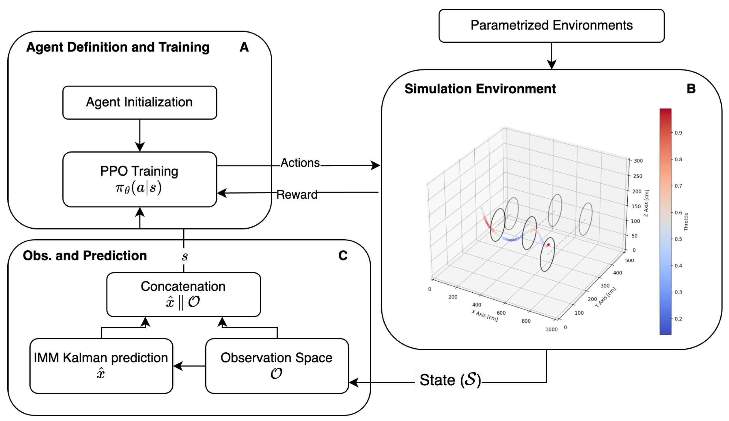
Figure 1. Method Overview: (A) Agent Planning Algorithm: Our approach computes the actions required by the agent, utilizing the observation space information. Learning is conducted in a reinforcement learning framework using the Proximal Policy Optimization (PPO) algorithm, with actions evaluated within the simulation environment. (B) Simulation Environment: Actions taken by the agent generate trajectories, which are evaluated for validity and scored according to a reward function based on inputs such as the agent’s position with respect to the dynamic gates of interest. (C) Observation Space and Gate Estimation: The simulation environment also captures the state at specific moments, enriching it with predictions from the IMM Kalman filter, which estimates the future positions of the gates. This predictive capability informs decision making in step (A), guiding the agent on the next actions to achieve the end goal of passing through all gates.
Aerospace 11 00395 g001
Figure 2. Overview of the simulation environment and the movable gates. In the image, the gray circle represents the object’s initial position, the black circle represents the final position, and the dashed line depicts the path taken by the object’s center as it moves through three-dimensional space.
Aerospace 11 00395 g002
Figure 3. Visualization of the reward function over time, showing non-linear penalty function, reinforcing optimal path planning, and highlighting jumps from rewards per gate passed and episode completion.
Aerospace 11 00395 g003
Figure 4. Absolute observed error between the predicted and simulated gate’s center position at the crossing time for a given episode is detailed. An increase in error is noted when the IMM filter transitions to target the next gate. However, this error quickly reduces to below 5 percent, indicating rapid adjustment and improved prediction accuracy post-transition.
Aerospace 11 00395 g004
Figure 5. To evaluate learning efficiency and stability over numerous training steps, this figure reports episode reward and episode length. Raw data (dots), rolling average (solid line, window of 10), and standard deviation (shaded areas, blue and red for two series) provide detailed insights into trends and variations in performance.
Aerospace 11 00395 g005
Figure 6. Three-dimensional trajectories of the drone’s navigation through the gates, with a color gradient representing the throttle’s magnitude on the x-axis. This visual representation elucidates the complex interplay between the drone’s velocity and its successful passage through the gates, thus highlighting the simulation environment’s role in advancing navigational tactics. Altogether, these visualizations provide a comprehensive overview of the drone’s behavioral dynamics and the effectiveness of the path-planning algorithms within our custom-designed simulation framework.
Aerospace 11 00395 g006
Figure 7. Visualization of the agent’s trajectory for different training steps, showing progressively optimized and faster performance in flying through the gates with more training steps.
Aerospace 11 00395 g007
Figure 8. ‘Action plots over the episode’, which illustrates the normalized action values across the episode steps for the X (blue), Y (green), and Z (red) axes, offering insights into the control strategy of the drone’s trajectory during navigation. The values reported here are normalized between 1 and −1, with 1 indicating movement in the positive direction of the axis and 1 indicating movement in the negative direction.
Aerospace 11 00395 g008
Figure 9. This heatmap illustrates the impact of varying speed multipliers (to be applied to the nominal condition) for the drone and gates on the success rate of an autonomous drone navigation system. Each cell represents the success rate (as the main value) and its standard deviation (as the small value with the ± sign), given a specific combination of gate and drone speed multipliers. The drone’s speed multiplier is indicated along the x-axis, while the gate’s speed multiplier is on the y-axis. Darker green shades signify higher success rates, indicating better performance under those speed conditions. As the multipliers increase, indicating faster speeds, the success rates vary, revealing how speed changes affect the drone’s ability to navigate through moving gates successfully.
Aerospace 11 00395 g009
Table 1. Environment description. This table provides an overview of the environment’s dimensions and significant areas.
ParameterValue
Maximum x Dimension [m]10.0
Maximum y Dimension [m]5.0
Maximum z Dimension [m]3.0
Agent Spawn Area [m] (x, y, z) 1(2.0, 5.0, 3.0)
End Episode Area [m] (x, y, z) 2(9.5, 5.0, 3.0)
1 Area used to limit the agent spawn; 2 Area defining the successful end of an episode.
Table 2. PPO algorithm parameters used as part of the training of the agent.
ParameterDescriptionValue
learning_rateLearning rate, can be a function 3 × 10 4
n_stepsSteps per environment per update2048
batch_sizeMinibatch size64
n_epochsEpochs when optimizing loss10
gammaDiscount factor0.99
gae_lambdaTrade-off bias/variance in GAE0.95
clip_rangeClipping parameter, can be a function0.2
normalize_advantageNormalize advantage or notTrue
ent_coefEntropy coefficient0.0
vf_coefValue function coefficient0.5
max_grad_normMax gradient norm for clipping0.5
use_sdeUse state-dependent explorationFalse
sde_sample_freqSample frequency for gSDE noise matrix−1
stats_window_sizeWindow size for rollout logging100
Table 3. Nominal simulation parameters and results over the metrics defined above.
ParameterValue
Agent’s Max Translation Speed [x, y, z] (cm/s)[15.0, 10.0, 10.0]
Gates Speed (cm/s)3.0
Success Rate (%) 87 ± 3.1
Average Reward per Action 11.60 ± 2.60
Disclaimer/Publisher’s Note: The statements, opinions and data contained in all publications are solely those of the individual author(s) and contributor(s) and not of MDPI and/or the editor(s). MDPI and/or the editor(s) disclaim responsibility for any injury to people or property resulting from any ideas, methods, instructions or products referred to in the content.