1. Introduction
The phenomenon of shimmy is a self-excited lateral yaw oscillation that can occur during the takeoff, landing, or taxiing of an aircraft’s landing gear. It is caused and sustained by the transfer of kinetic energy from the aircraft to the landing gear. In order to effectively address significant issues in the design of anti-swing mechanisms for aircraft landing gears, it is crucial to have a comprehensive understanding of the mechanism behind shimmy and investigate how various factors impact its stability [
1]. The issue of shimmy has always posed a formidable challenge in the design and operation of aircraft landing gears. Mastering the accurate and appropriate analysis of shimmy dynamics is pivotal in addressing the oscillation problems associated with shimmy [
2].
Liu [
3] found that shimmy is primarily caused by the torsional mode of the wheel’s swinging part around its directional axis and the lateral bending mode of the landing gear around its longitudinal axis. The longitudinal mode, on the other hand, has minimal impact. At the same time, the tire and ground contact areas experience alternating deformation, and the oscillation of the wheel can cause the landing gear strut and the fuselage to shake, potentially resulting in the entire fuselage trembling, on the basis of the mechanics of the landing gear and linear models of the tire elasticity. Somieski [
4] applied well-known linear mathematical methods to analyzing the shimmy of a basic nose landing gear model and investigated the impact of various structural parameters on the shimmy dynamics. Tartaruga [
5] performed sensitivity and uncertainty analysis using singular value decomposition to investigate the impact of various structural parameters on shimmy onset. The results indicate that the proposed method reduces the computational time compared to full-scale full element simulation. The study conducted by Thota et al. [
6] examined a seven-dimensional landing gear model encompassing torsional, lateral, and longitudinal degrees of freedom. Their analysis focused on the overall shimmy behavior and frequency, revealing that variations in the forward velocity and vertical force influence the interaction between the torsional mode and lateral bending mode, resulting in diverse types of shimmy phenomena. Conversely, minimal involvement was observed from the longitudinal mode regarding any potential occurrence of shimmy.
The landing gear is a complex structural system characterized by the high nonlinearity arising from the nonlinear deformation of tires, elastic tire deformation, and side slip [
7]. The nonlinearities in the landing gear include shock absorbers, dampers, joint free clearance, and coulomb friction components [
8,
9], which contribute significantly to nonlinear vibrations. From a dynamics perspective, bifurcation phenomena primarily encompass saddle node bifurcation, transcritical bifurcation, pitchfork bifurcation, period-doubling bifurcation, and Hopf bifurcation [
10]. Among these types of bifurcation, Hopf bifurcation is closely associated with the limit cycles and self-excited vibration within the system; thus, it represents a dynamic form of bifurcation. Shimmy motion corresponds to periodic solutions in nonlinear dynamics that typically emerge due to Hopf bifurcations. Consequently, it holds substantial research value.
Thota et al. [
11] distinguished the stable region from the shimmy oscillation region by means of the Hopf bifurcation curve. They classified different types of shimmy as torsional, lateral, and quasi-periodic shimmy. Ghadami [
12] proposed an effective method for predicting Hopf bifurcation and analyzing the complete post-bifurcation behavior of nonlinear oscillatory systems. By measuring the system’s response to a disturbance in its pre-bifurcation state, a three-dimensional bifurcation diagram was generated for prediction purposes. The advantages of this prediction method were demonstrated by utilizing the predicted bifurcation diagram of a fluid structure system, which accurately predicted both supercritical and subcritical bifurcations. Thota et al. [
13] investigated a nose gear model with a two-wheel configuration. They selected forward velocity and vertical load as the bifurcation parameters and analyzed how structural parameters influenced two types of shimmy. Additionally, they provided transformations between different two-parameter bifurcation diagrams. The research revealed that besides stable torsional shimmy and stable lateral vibration, it could also trigger quasi-periodic shimmy. Li [
14] studied the Hopf bifurcation of an aircraft nose landing gear model based on two pairs of continuous parameters. The results showed that higher-order terms caused deviations between the original system’s bifurcation curve and truncated amplitude system’s bifurcation line. This deviation led to a contraction in the bistable region compared to in previous findings.
In recent years, extensive research has been conducted on Hopf bifurcation and the central manifold of nonlinear dynamical systems. Zhang [
15] proposed a model for a piecewise smooth suspended single wheelset, investigating the influence of the vehicle parameters on the characteristics of Hopf bifurcation. By employing the central manifold theorem, they successfully reduced the dimensionality of the wheelset equation and derived an expression for the first-order fine focus. Dong [
16] utilized the normal form method to demonstrate that high-speed EMUs exhibit subcritical and supercritical Hopf bifurcations under simplified wheel–rail contact relationships. Additionally, Dong identified the factors contributing to the distinct types of bifurcations observed in two types of bogies. Sandor Beregi [
17] employed a brush tire model to analyze the nonlinear dynamics of traction wheels by reducing its center manifold into a normal form comprising linear and piecewise smooth second-order terms. This normal form was used to establish stability at non-hyperbolic equilibrium points within the system and provided an estimate for the limit cycles appearing at linear stability boundaries. It has been proven that subcritical Hopf bifurcations in non-smooth delay systems generate parameter ranges with bistability that is undetectable using standard tire models. Wang [
18], using the vehicle speed as a bifurcation parameter, applied central manifold theory to obtain a two-dimensional central manifold at critical vehicle speeds in order to comprehensively analyze the characteristics of Hopf bifurcation in shimmy systems while obtaining an approximate periodic solution.
The current research on the stability of aircraft nose landing gear has advanced from linear stability theory to nonlinear bifurcation theory [
19,
20]; however, there remains a lack of comprehensive explanations and solutions for certain fundamental shimmy problems encountered in practical applications. Furthermore, the analysis of shimmy problems has not yet considered the central manifold method. This article employs a combination of theoretical derivation and numerical simulation to analyze a landing gear system that incorporates higher-order nonlinear factors. The center manifold simplification method is utilized to streamline the nose landing gear system, while the position of the equilibrium point is examined using classical linear theory. The Hopf bifurcation of the equilibrium point is investigated using classical bifurcation theory, with its specific type determined based on the first Lyapunov coefficient. Both numerical simulation and theoretical derivation mutually validate each other’s findings. The research results presented in this article can serve as valuable theoretical references for optimizing the structural design of aircraft landing gear shimmy dynamics systems.
2. Dynamic Modeling of Nose Landing Gear Shimmy
2.1. Coordinate System and Degrees of Freedom
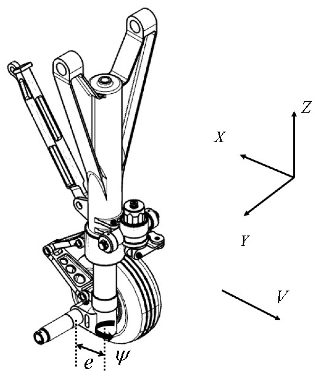
The stability of shimmy is influenced by various factors, including linear parameters such as stability distance, tire characteristics, and aircraft taxiing speed and non-linear factors such as damping, friction, and clearance. In order to investigate the impact of key parameters on the shimmy behavior, this study employs a simplified model of the nose landing gear in a two-wheeled aircraft equipped with an oil damper under a specific vertical load, as shown in
Figure 1:
The landing gear follows the fuselage at a constant speed V, with the reverse direction of the taxiing defined as the X-axis of the landing gear coordinate system. The Y-axis represents horizontal movement to the right and the Z-axis represents vertical movement upward. The landing gear strut torsion is in a neutral position, so any lateral motion of the fuselage is not taken into consideration. During smooth taxiing, the aircraft does not experience any vertical displacement, and the stroke of the landing gear buffer remains constant. Therefore, the vertical displacement of the landing gear is not taken into account.
- (1)
The landing gear strut can rotate around the directional axis with an angle of .
- (2)
In the X-axis direction, it is considered that the stiffness of the landing gear strut is sufficient, and the deformation has a small impact on the shimmy.
- (3)
The lateral displacement of the left and right tires is used to describe the deformation of the tires.
- (4)
The degree of freedom of the axle torsion deformation indicates that the two wheels do not rotate together.
Due to the fact that the strut does not have a forward inclination angle, the tire angle is the same as the landing gear strut angle. Under a small angle rotation, assuming that there is no change in the vertical load on the two wheels, it can be considered that the lateral and torsional deformations of the two tires are the same. For the convenience of subsequent calculations, the stiffness of the two tires is superimposed and set as the stiffness damping parameter of a single tire.
2.2. Tire Dynamics Model
In Smiley’s tire mechanics theory, the forces and moments exerted by the ground on the tire can be expressed as:
where
and
are the lateral stiffness and damping coefficients of the tire, respectively;
and
are the torsional stiffness and damping coefficient of the tire, respectively; and
and
are the lateral elastic deformation and torsional elastic deformation of the tire, respectively.
As shown in
Figure 2,
and
can be expressed in the following form:
is the lateral displacement of the tire’s touchdown center point while
is the landing gear stability distance. Smiley’s theory uses Taylor series, ignoring the higher-order terms in the series, and can form different tire approximate constraint equations. This article adopts Smiley’s second-order approximation formula:
In the equation, ,. is the half length of the tire touching the ground; is the tire slack length.
We calculate the tire formula using equation coordination:
2.3. Nonlinear Analysis of Pendulum Reducers
The torsional damping moment provided by anti-swing dampers typically exhibits a nonlinear relationship with the swing speed of the column’s torsional degrees of freedom. During the front wheel shimmy process, the oil in the stabilizer is confined to enclosed circuits such as damping pipelines and throttling devices. The damping pipeline of a pendulum reducer generally adopts a circular cross-section. Ideally, the damping torque of the pendulum reducer demonstrates a quadratic power function characteristic. In reality, however, factors such as temperature and fluid boundary layer effects may result in high-power damping as well. The torsional anti-swing damping torque provided by the pendulum reducer can be roughly described as follows:
, , and are the linear term torsional damping coefficient, square term torsional damping coefficient, and cubic term torsional damping coefficient, respectively.
When considering the square term in nonlinear damping, its inclusion of a sign function poses challenges for analysis. Within the range of small angle vibrations, cubic damping also exhibits an increasing trend with angular velocity. In terms of the nonlinear influence properties, studying cubic damping can serve as a substitute for investigating square term damping.
2.4. Dynamic Equations of the System
The dynamic equilibrium equation for the torsion direction of the pillar is:
Make
. The equation can be represented as a system of first-order differential equations, as follows:
where:
The parameters of the nose landing gear of the aircraft used in this study are shown in
Table 1:
3. Hopf Bifurcation Theory of the Oscillation Model
3.1. Linear Stability Theory
Before conducting stability analysis on the nose landing gear system, it is imperative to initially acquire the eigenvalues of the linearized system at the equilibrium point. The characteristic equation of the linear component within the dynamics equation pertaining to the landing gear can be expressed as follows:
In the equation,
is the fourth-order identity matrix, and
λ represents the characteristic root of the landing gear system. Expanding the equation yields:
In the equation,
is the coefficient of each order of the characteristic equation, expressed as follows:
When calculating the linear critical speed of the landing gear system, there are typically two methods available: the root trajectory method and the Hurwitz stability criterion method. In comparison to the root locus method, the Hurwitz stability criterion method eliminates the need to solve the characteristic roots of the system equation. Instead, it solely relies on determining the system motion stability based on the coefficients within the characteristic equation [
21]. The Liénard–Chipart stability criterion adopted in this paper further simplifies the calculation process based on Hurwitz [
22].
The Hurwitz matrix is as follows:
According to the Liénard–Chipart stability criterion, the necessary and sufficient conditions for the characteristic equation to have a pair of pure imaginary roots and the other two roots to have negative real parts are:
When , the system is in a critical stable state, and when , the system is in a convergence state.
3.2. Hopf Bifurcation Theory
According to the Hopf bifurcation criterion, the necessary conditions for Hopf bifurcation are as follows:
According to the practical significance of the structural parameters of the landing gear, it is easy to verify
; from this, it can be seen that when
is satisfied, it is the critical state of landing gear system equilibrium point instability, and the univariate quantic equation of speed can be obtained:
where
is the coefficient of each order, and the expression is as follows:
The smallest positive real root of all solutions of the equation is the linear critical speed of the landing gear system. At the Hopf bifurcation point of the nose landing gear system, the characteristic equation has a pair of pure imaginary roots
, where
, because
is the root of the characteristic equation. We bring
into the characteristic equation to obtain:
Since the real part is zero, we have:
So, the characteristic equation is decomposed into:
According to the equal coefficient of the same term:
When the discriminant satisfies
, a pair of eigenvalues with negative real parts of the characteristic equation can be obtained,
, where
. The specific expression is as follows:
When the discriminant satisfies , a pair of real root eigenvalues of the characteristic equation can be obtained: .
3.3. Dimension Reduction in the Central Manifold Theorem
If the bifurcation characteristics of the high-dimensional system are directly analyzed, the process is cumbersome, and the dimensions of the high-dimensional system can be reduced to the plane system using the central manifold theorem [
23]. Then, the analysis method of the plane system is used to complete the research on the high-dimensional system. When the current landing gear equation is at a critical speed, let
be the eigenvector of matrix
corresponding to eigenvalue
. Take two eigenvalues containing imaginary parts as an example: let
be the eigenvector of matrix
corresponding to eigenvalue
. Then,
satisfies the following equation:
where the expression of
is as follows:
Before applying the central manifold theorem, first, the real eigenbasis matrix
is constructed by using the eigenvector
, and then the landing gear equation is transformed into the Jordan canonical form using matrix
. Matrix
is as follows:
For the convenience of symbol derivation, matrix
is recorded as:
Let
where
be substituted into the landing gear equation and finally transformed into the Jordan standard:
For the critical point of Hopf bifurcation, there are two eigenvalues of the Jordan type matrix with zero real parts and one with negative real parts.
And because
, then there is a central manifold
,
,
, and we define the operator:
It can be seen from
that
is a nonlinear function of no less than order 3, and the Taylor expansion of the central manifold is as follows:
We bring the equation into the operator and merge the terms with the same degree. Since the coefficient is 0, eight equations and eight unknowns are obtained, which can be solved into the
coefficient. Considering that only quadratic and cubic terms of the state variables are needed to calculate the first Lyapunov coefficient, the higher-order term system of the central manifold is ignored, and the final dimension reduction is as follows:
In order to judge the Hopf bifurcation type of the shimmy system and investigate the limit cycle stability of the system, the stability parameter of the central manifold is introduced:
The central popular stability parameter is obtained as .
3.4. Analysis of the Time-Delay Effect under Linear Damping
Hopf bifurcation refers to the phenomenon of periodic motion that arises from the equilibrium state when the bifurcation parameters cross the bifurcation point. In order to distinguish the type of Hopf bifurcation in the landing gear system, this section utilizes canonical theory to derive the discriminant for identifying the type of Hopf bifurcation in the landing gear system [
24].
When Hopf bifurcation occurs in the landing gear system, there is a pair of pure imaginary roots in the equation
. Let
be the right and left eigenvectors of matrix
: then,
satisfies the following equation:
Normalize
to
; then, at this time:
By solving the above equations together, it can be obtained that:
Introducing complex variables
, any vector in the equation
can be uniquely represented as
: we bring it into the available:
is expressed in the Taylor series form of conjugate complex variable
as follows:
From the equality of the power coefficients of the same degree, it can be concluded that:
The first-order fine focus
of the system is as follows:
The first Lyapunov coefficient can be obtained as:
When , supercritical Hopf bifurcation occurs in the landing gear system. When , the undercarriage system undergoes subcritical Hopf bifurcation. When , the first Lyapunov coefficient degenerates, and the landing gear system degenerates the Hopf bifurcation. Since it is greater than zero, the central popular stability parameter and Lyapunov coefficient have the same sign, so it is accurate to judge the type of Hopf bifurcation.
4. Stability Analysis of Oscillation System
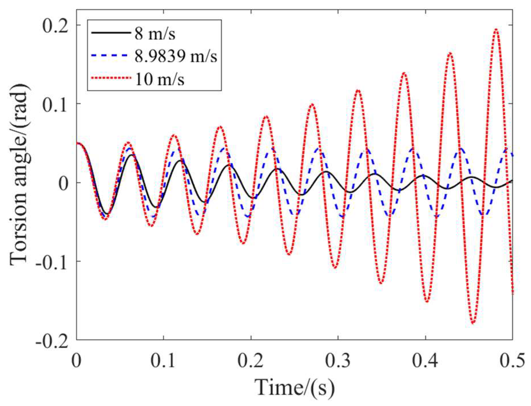
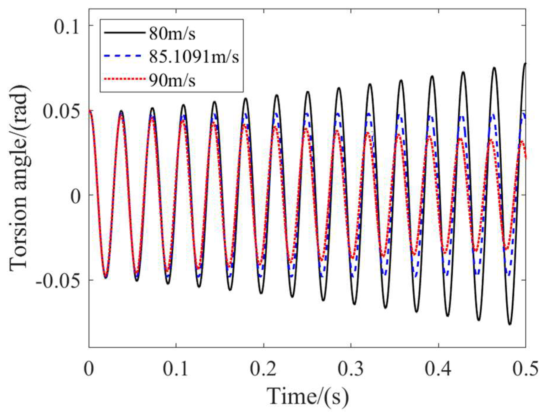
4.1. Numerical Verification of the Theoretical Results
To verify the accuracy of all the derived formulas, given the parameter values, in addition to the parameters in
Table 1, we set the linear damping coefficient C = 10 Nms, substitute it into the formula, and calculate it to obtain
= 1.2375 × 10
7,
= −1.0603 × 10
9,
= −2.6470 × 10
6,
= 4.8429 × 10
10, and
= 2.5335 × 10
11. By simplifying the equation, it can be concluded that:
Taking the roots of the equation yields the following five roots: 85.1091 + 0.0000i, 8.9839 + 0.0000i, −4.2065 + 3.0134i, −4.2065 − 3.0134i, 0. The smallest positive real roots 8.9839 and 85.1091 in the solution are the linear critical speeds of the landing gear system. We select speed points near the speed for analysis as follows:
The stability analysis of time-delay systems, similar to their non-time-delay counterparts, can be primarily categorized into two methods: time-domain and frequency-domain approaches. The key advantage of the time-domain analysis method lies in its ability to effectively handle system nonlinearity and uncertainty. By setting the time delay as 0 ms, 3 ms, and 4 ms, the simulation results are depicted in the
Figure 3 and
Figure 4 below.
At the critical speed point, the swing angle of the landing gear exhibits constant amplitude vibration. When the speed value is slightly changed, the system’s state either becomes divergent or convergent, thus verifying the accuracy of the derived formula.
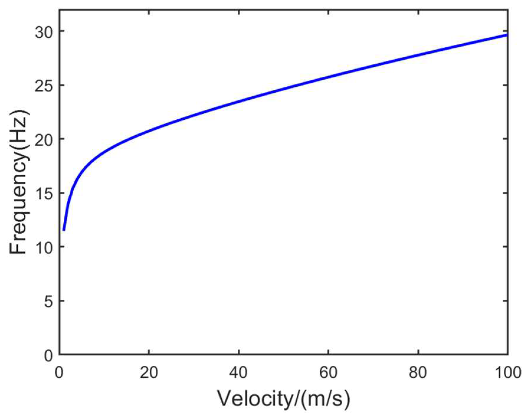
Shimmy primarily involves the stability and frequency of a system, with stability being just one factor in determining the criticality of the system. Consistency in frequency can ensure the accuracy of the theoretical results. According to the analysis in the previous section, the frequency expression of oscillation is as follows:
Therefore, the relationship between frequency and speed is shown in the following
Figure 5:
According to the calculations, the oscillation frequencies corresponding to the two critical speeds are 18.483 Hz and 28.266 Hz, respectively.
The FFT algorithm is a fast algorithm for the discrete Fourier transform, which transforms the time-domain signals into frequency-domain signals. By analyzing the frequencies of time-domain, it can be observed that the frequencies of the two are 18.5 Hz and 28.3 Hz, respectively. It can be seen that the values of the two are similar. In summary, the numerical analysis results are consistent with the aforementioned analytical analysis results, confirming the accuracy of the model and the effectiveness of the analytical method.
4.2. The Influence of the Stability Distance on the Stability of Shimmy
The landing gear, being a complex mechanical dynamic system, exhibits significant coupling effects among its various components and subsystems. Consequently, there exist numerous factors that influence the aircraft shimmy, along with diverse engineering approaches to mitigating landing gear shimmy. However, parameters such as the tire radius, lateral stiffness, and equivalent mass of the entire nose landing gear pose challenges in terms of adjustment and optimization within engineering practice. The stability distance holds paramount importance in shimmy analysis as it plays a crucial role in suppressing shimmy by generating a restoring torque on the landing gear strut through the lateral force exerted on the tire due to its stable distance from the ground. In light of this significance, this article primarily focuses on investigating the geometric stability distance of the landing gear, which can be easily adjusted. The objective is to provide technical guidance for enhancing anti-shimmy design in engineering practice.
Due to the large overall mass of the tire, changes in the stability distance can lead to changes in the inertia around the axis. Assuming a wheel and axle mass of 10 kg, the total rotational inertia of the piston rod, torsion arm, and other rotating components around the pillar
= 0.186 kgm
2, and we have:
When the damping of the anti-swing damper and the structural damping are not considered, then
. Therefore, it can be obtained that:
In addition to having two zero roots in the speed, there are also two other ones:
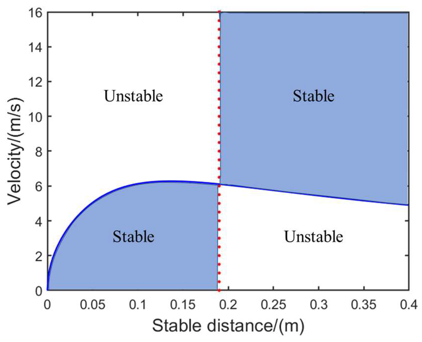
Due to all the parameters being greater than zero, there is a constant critical velocity in the system without considering damping dissipation, which stabilizes the system. We name the sum of the half length of the tire touching the ground and the slack length as the critical stable distance or climbing distance. When the stable distance is less than the crawling distance, we have , and the stability interval of the system is ; when the stable distance is equal to the creep distance, we have , and the stability interval of the system is ; and when the stable distance is less than the crawling distance, we have , and the stability interval of the system is . Therefore, it is possible to draw a stability zone map corresponding to the landing gear stability distance and speed.
From
Figure 6, it can be observed that the aircraft remains stable during taxiing at a certain speed when the distance between the tires is greater than the combined length of half of the tire in contact with the ground and the slack length. Therefore, when the problem of aircraft shimmy is extremely prominent, lengthening the landing gear stability distance or switching to smaller-sized tires can be considered.
4.3. Analysis of Shimmy Stability
After the completion of a general landing gear design, modifying its structure poses significant challenges. This modification process entails addressing various aspects, including the dynamic stability performance, static strength concerns, retraction and extension issues, as well as the spatial and fuselage layout of the landing gear cabin. To effectively resolve nose landing gear shimmy while minimizing any impact on the other components, the installation of anti-shimmy dampers is deemed the most efficient approach.
In order to determine the maximum critical damping coefficient, Shen Tianheng was inspired by the formula for finding the root of a one-dimensional quartic equation. He simplified the formula and provided a more convenient criterion for determining the number of real number solutions and the case of multiple roots of the equation. Moreover, Tianheng’s formula does not involve imaginary number square roots, which simplifies the operation and makes it more convenient. This also allows for simplification of the code in computer root-finding tools. For equations
, the double root discriminant is:
When , , the equation has a pair of double real roots; if , the other two are conjugate imaginary roots, and .
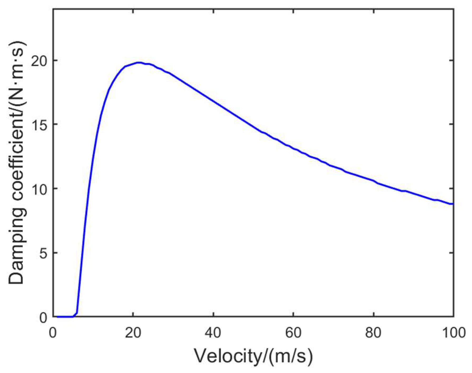
is a complex expression containing the damping coefficient , which contains the high-order coefficient. In order to obtain the critical value concisely and quickly, the dichotomy method is used to change the damping coefficient value. By judging the sign of , the critical damping coefficient is obtained. Finally, after iteration, is 19.8389 Nms. Substituting this value into the characteristic equation, its root can be calculated as y = 21.4322 + 0.0000i, 21.3154 + 0.0000i, −5.4031 + 3.9523i, −5.4031 − 3.9523i. Therefore, in the full speed domain, the maximum required damping corresponds to a speed of approximately 21.4 m/s. As long as the damping coefficient of the stabilizer is greater than 19.8389 Nms, the landing gear oscillation is stable.
To validate the aforementioned conclusion, it is imperative to initially perform a dual parameter analysis of the critical stable state of the landing gear system in order to conduct linear stability analysis of the shimmy. This analytical process entails modifying the values of both the speed and damping coefficient within the system. By means of time-domain analysis and numerical computation, the following can be deduced.
As shown in
Figure 7, the analysis reveals that the required anti-swing damping force of the system initially increases and subsequently decreases as the speed escalates. Notably, at a velocity of 21.4 m/s, the maximum damping is achieved with an anti-swing damping value of 19.9 Nms, which aligns consistently with the previous findings. Consequently, it can be inferred that this velocity damping coefficient curve represents the critical damping coefficient essential for ensuring the landing gear’s oscillation stability. Remarkably, the peak critical damping value corresponds to the minimum requirement for overall system stability across all speeds.
4.4. Hopf Bifurcation Analysis
The forward taxiing speed of an aircraft is also an important factor affecting shimmy. Usually, the landing gear system is prone to inducing shimmy within a certain speed range during forward sliding, known as shimmy speed. According to the critical speeds of 8.9839 m/s and 85.1091 m/s calculated in the previous section, the two parameters are substituted into the nonlinear analysis: for the critical speed of 8.9839 m/s, their corresponding eigenvalues are
and
. The calculated
is −0.0077. We obtain the first Lyapunov coefficient of the landing gear system according to the formula
; from this, it can be determined that when the speed exceeds 8.9839 m/s, the landing gear system undergoes supercritical Hopf bifurcation. Similarly, for speeds of 85.1091 m/s, their corresponding characteristic values are
,
, and the calculated
is −0.0061. We obtain the first Lyapunov coefficient of the landing gear system according to the formula
, and from this, it can be determined that a supercritical Hopf bifurcation occurs in the landing gear system when the speed is below 85.1091 m/s. In order to verify the correctness of the theoretical calculation results, the differential equation of the landing gear system was numerically solved to obtain the curve of the maximum real part of the eigenvalues of the landing gear system under the parameters in
Table 1 as a function of the sliding speed, as shown in the
Figure 8:
From the
Figure 8, it can be observed that the maximum real part of the eigenvalues initially decreases as the sliding speed increases. It reaches the minimum value at a speed of 4.65 m/s. Then, it starts to increase again. At a speed of 8.9839 m/s, the maximum real part of the characteristic value of the landing gear system crosses the zero point, changing the stability of the equilibrium point of the landing gear system. This indicates that the minimum critical speed of the landing gear system is 8.9839 m/s. As the speed further increases to 23.95 m/s, the maximum value is reached. Finally, the real part of the system’s eigenvalues gradually decreases. At a speed of 85.1091 m/s, the maximum real part of the eigenvalues of the landing gear system crosses the zero point again, this time from positive to negative, indicating another change. In terms of the stability of the landing gear system, the maximum critical speed is determined to be 8.9839 m/s. The simulation results align with the theoretical calculations, thus confirming the accuracy of the theoretical analysis method presented in this paper.
During the forward taxiing process of an aircraft, shimmy occurs when the parameter values are located at the Hopf bifurcation point of the shimmy dynamics equation. Strictly speaking, it must be a supercritical Hopf bifurcation. In this case, any minor external excitation or disturbance can cause the system to oscillate.
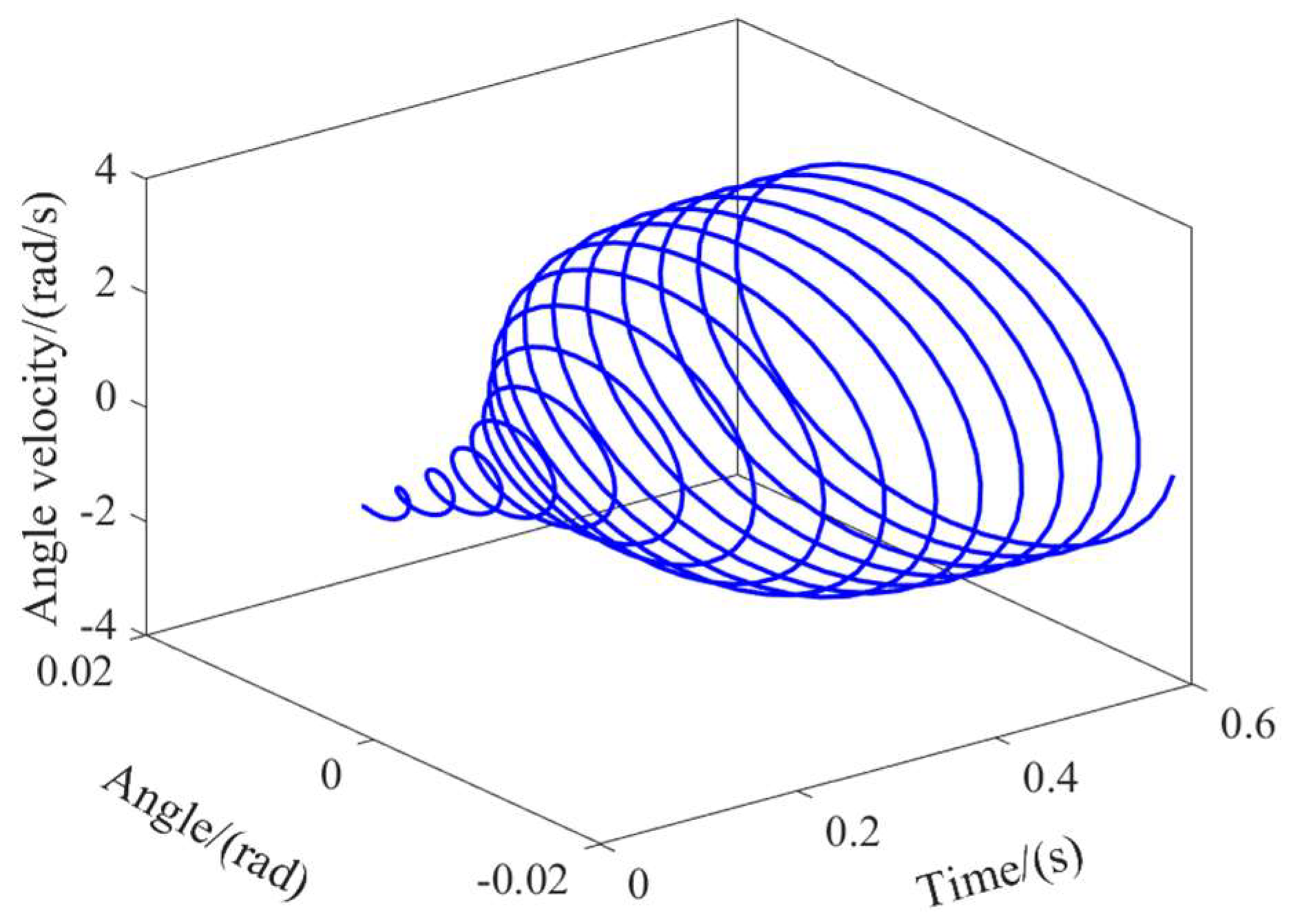
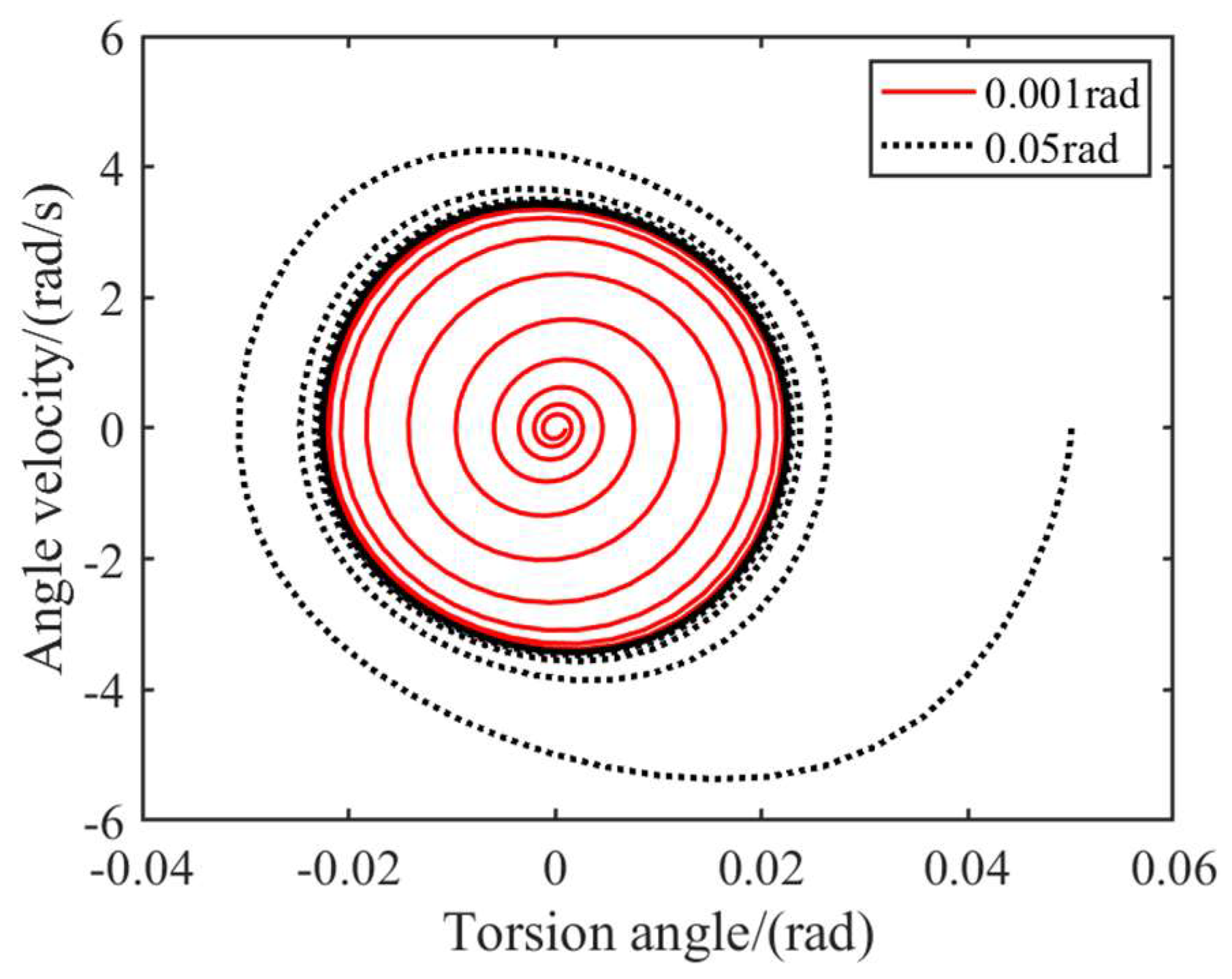
We set the sliding speed to 30 m/s, the linear damping coefficient = 10 Nms, the nonlinear damping coefficient = 1 Nms3, and the initial swing angle to 0.001 rad. The following curve can be obtained using numerical simulation:
As can be seen in
Figure 9, at the current parameter value, the system will gradually approach a state of constant amplitude vibration due to the non-zero initial conditions, leading to the loss of stability in the original neutral equilibrium state. The axes in the phase space represent different state parameters of the system. A point in the phase space signifies the system’s state, while its trajectory forms a phase orbit depicting the evolution of the system’s state over time. Drawing a phase diagram involves representing spatial coordinates for each degree of freedom at a specific time point, enabling analysis of the dynamic motion trends across different spatial states.
Based on the phase diagram of
Figure 10, it is evident that the incorporation of non-linear damping into the system results in the convergence of the landing gear swing angle’s amplitude to a constant value during motion progression, irrespective of the initial conditions. Furthermore, all the trajectories depicted in the system phase diagram gradually approach a limit cycle. The presence of nonlinear damping in the landing gear system can induce limit cycles, consequently leading to sustained oscillation.
4.5. The Influence of Parameters on Amplitude
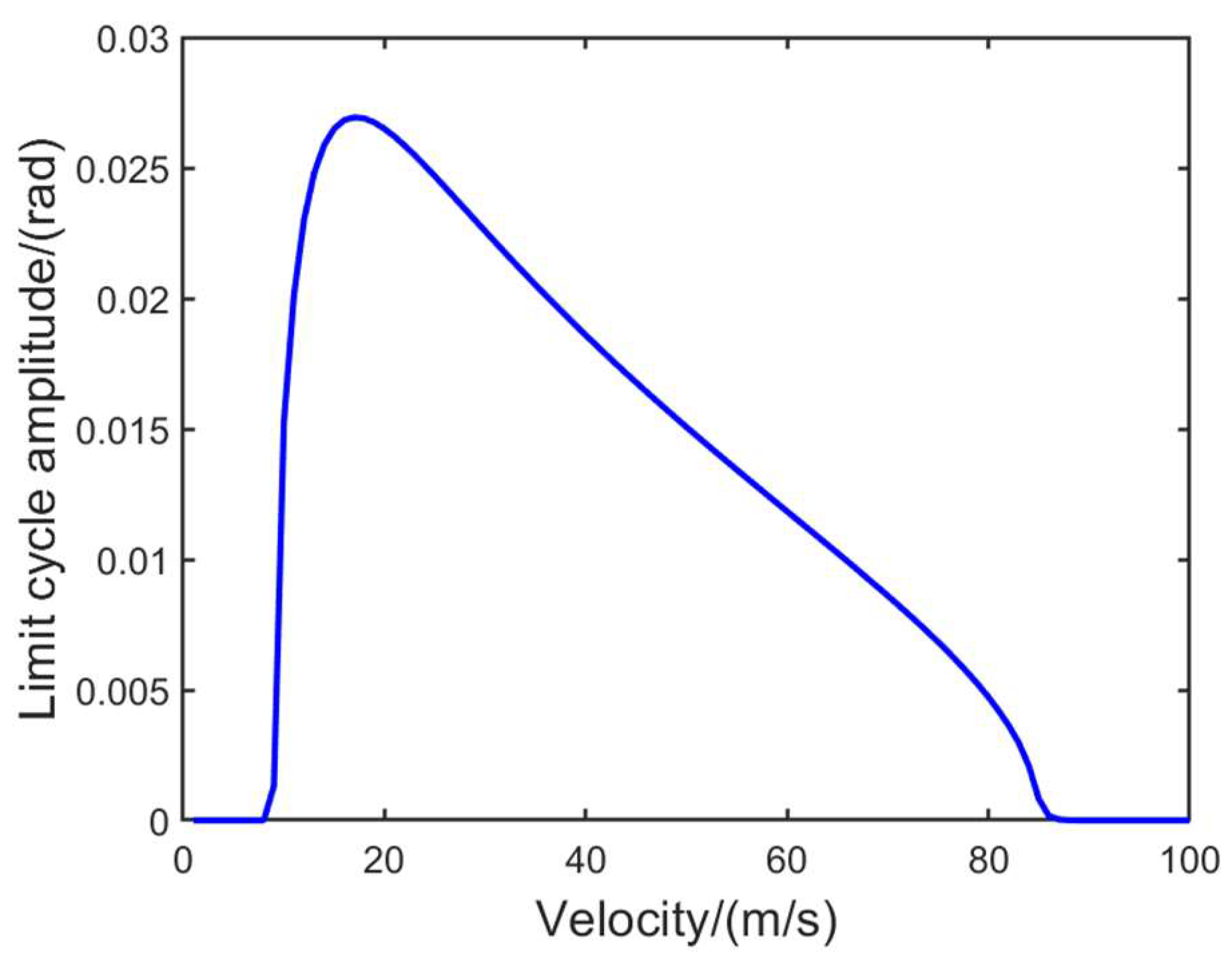
When the system undergoes Hopf bifurcation and generates limit cycles, it is necessary to restrict the range of the oscillation amplitude in order to mitigate aircraft sliding accidents. Theoretically, small constant amplitude vibrations can be effectively suppressed by Coulomb friction. Furthermore, considering the significant influence of the parameters on the limit cycle, it becomes imperative to investigate how parameter variations affect the amplitude of the limit cycle. Firstly, let us examine the impact of the aircraft taxiing speed on the limit cycle.
Observation
Figure 11, in systems that are unstable or potentially divergent, the occurrence of a stable limit cycle during motion is expected, as it helps maintain the system stability through constant oscillations. The bifurcation diagram reveals two supercritical Hopf bifurcations, but in opposite directions. Specifically, as the speed increases, a limit cycle begins to emerge, and its amplitude gradually increases until reaching its maximum value. However, with a further increase in speed, the amplitude of the limit cycle starts to decrease until it eventually disappears. Notably, for the first bifurcation value, the stable limit cycle appears on the right side, while for the second bifurcation value, it appears on the left side. These findings align with previous theoretical analysis.
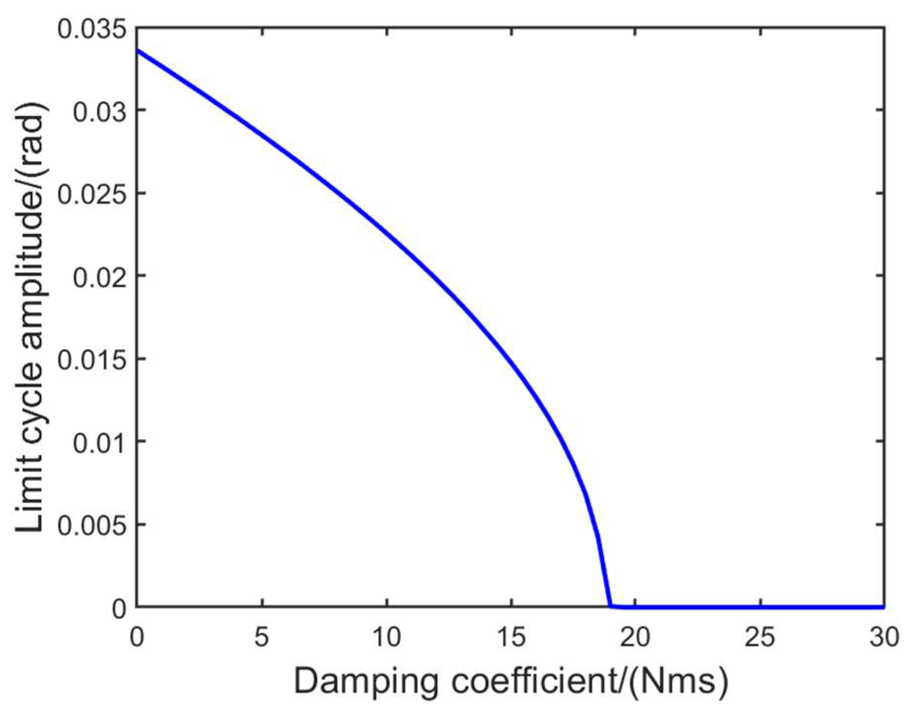
From the bifurcation diagram of
Figure 12, it can be seen that as the linear damping increases, the amplitude of the limit cycle begins to decrease. At a linear damping value of 19 Nms, the limit cycle disappears, and the system tends to stabilize. By comparing the results of the linear analysis, it can be observed that when the speed is 30 m/s and the damping coefficient is 19 Nms, all the real parts of the eigenvalues are negative, indicating that the system is stable and convergent.
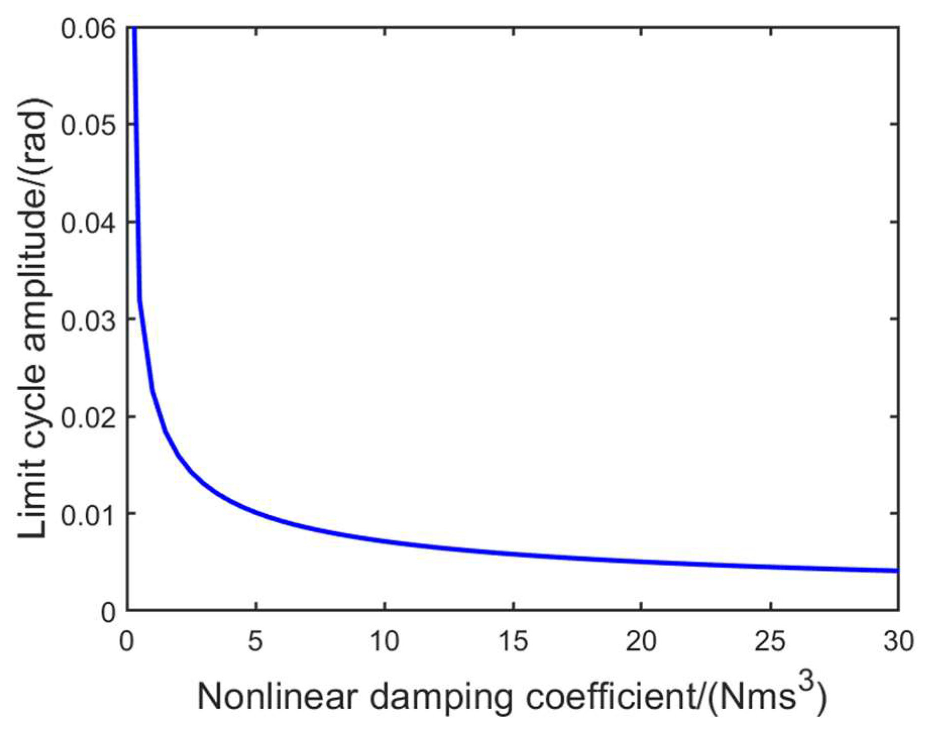
The primary factor leading to limit cycles in landing gear systems is the magnitude of the nonlinear damping coefficient. In the absence of nonlinear damping, linearly unstable systems would result in an unbounded increase in the landing gear swing angle, which contradicts the current scenario. However, it is observed that many landing gears experience structural damage or even aircraft instability due to excessive torsional deformation. Hence, a comprehensive investigation into the nonlinear damping coefficient across the entire amplitude range of oscillation limit cycle becomes imperative.
As illustrated in the
Figure 13, an increase in the nonlinear damping coefficient leads to a gradual reduction in the amplitude of the limit cycle within the system, thereby maintaining the stable state of the limit cycle. When the nonlinear damping coefficient is small, the amplitude of the limit cycle becomes significantly large. However, as the nonlinear damping increases, there is no direct proportionality between its increment and a decrease in amplitude of the limit cycle. Hence, it can be inferred that the presence of nonlinear damping alone ensures sustained low-amplitude vibration without necessitating deliberate adjustment of its coefficient.
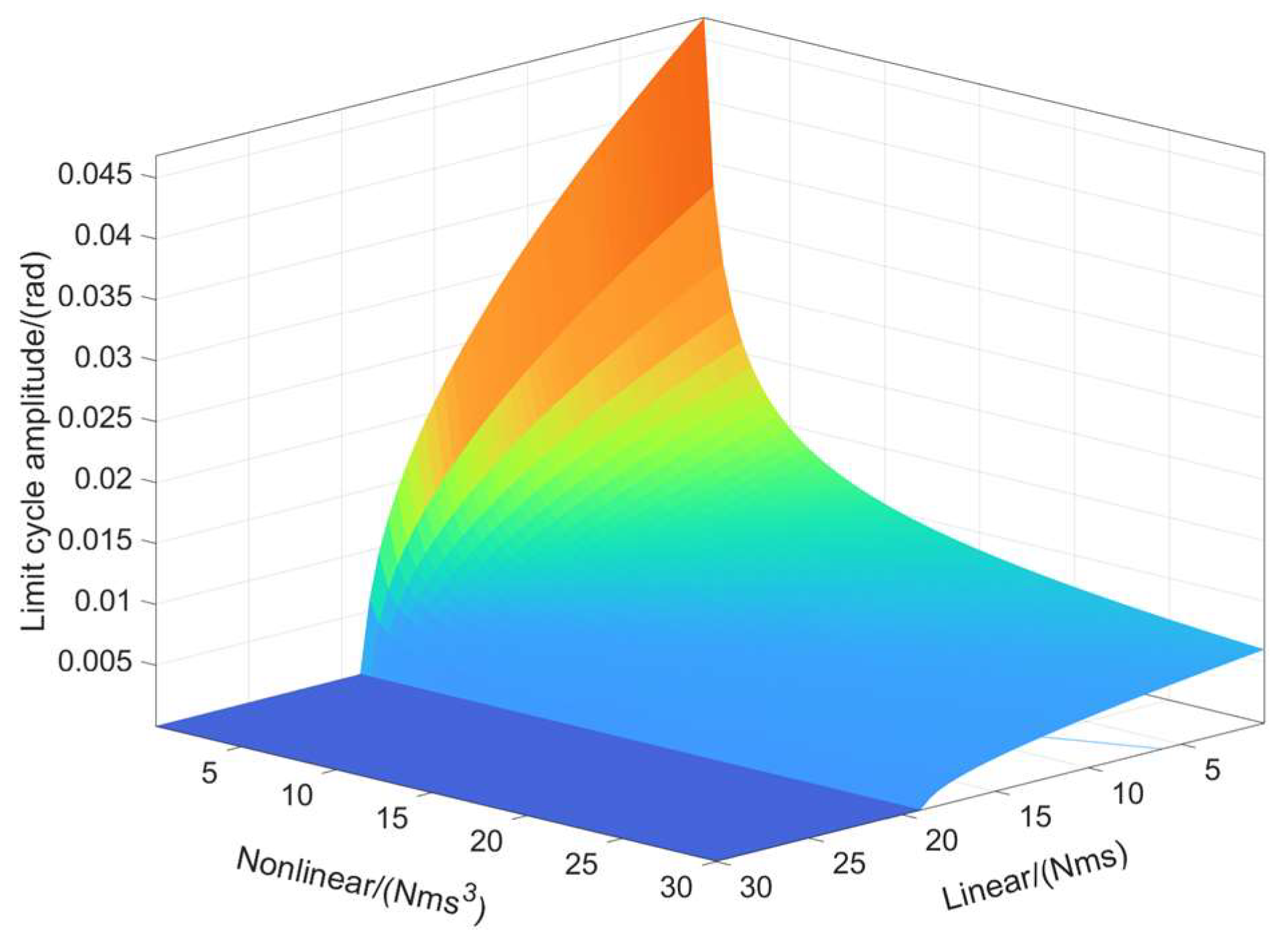
We distribute the nonlinear damping coefficient and linear damping coefficient within a specified range and analyze their impact on the amplitude of the limit cycle, as illustrated in the three-dimensional diagram above
Figure 14. The system can only stabilize and converge by increasing the linear damping coefficient. Moreover, during Hopf bifurcation, the amplitude of the limit cycle remains relatively small. In terms of nonlinear coefficients, a limit cycle is always generated when there is linear instability; however, this helps mitigate the aircraft sliding risks caused by continuous divergence of the system. Therefore, during the stabilizer design stage, it is crucial to consider both the existence and significance of the damping coefficients.


