Real-Time Ground Aeroservoelastic Test for Slender Vehicles Based on Condensed Aerodynamic Force Loading

Abstract

Slender vehicles often encounter significant aeroservoelastic challenges due to their low elastic mode frequencies and wide servo control system bandwidths. Traditional analysis methods have limitations, including low modeling accuracy for real vehicles in numerical methods, scale errors in wind tunnel tests, and significant risks in flight tests. The ground aeroelastic stability test is an innovative experimental method designed to address these challenges. This novel method employs shakers to apply condensed unsteady aerodynamic forces in real-time to actual vehicles, serving for both the ground flutter test (GFT) and the ground aeroservoelastic test (GAT). While extensive research exists on the GFT, there is limited exploration of the GAT. For the GAT of a slender vehicle in this paper, the condensed aerodynamic forces are calculated using the quasi-steady aerodynamic derivative method. An improved, partially decoupled inverse model controller is designed for force control, guided by an assessment of coupling strength among different shakers. Ground experiments under various flight control laws and flight dynamic pressures produce accurate results. Numerical simulations and experimental results demonstrate high precision, with excitation force amplitude deviations within ±10% and phase deviations within ±5° within the frequency range relevant to aeroservoelastic stability.

1. Introduction

Aeroservoelasticity (ASE) manifests as a complex interplay among unsteady aerodynamic forces, elastic structures, and servo control systems [1]. Slender vehicles, characterized by a high slenderness ratio, often exhibit low mode frequencies. Concurrently, the flight control system (FCS) and actuators possess high bandwidths to meet the demands for maneuverability. Consequently, ASE instability is a prevalent occurrence in slender vehicles, posing a potential threat to serious accidents.

The traditional ASE stability analysis methods can be broadly classified into two main categories: (1) Numerical methods [2,3] involve numerical modeling of the analyzed aircraft and its servo control system. This process requires introducing numerous assumptions across various aspects, such as the structure, aerodynamics, and servo control system, making it challenging when considering the various nonlinear factors and modeling errors that exist in reality. As a result, the analysis results have a limited reference value. It is worth noting that numerical models often require adjustments based on experimental results to enhance modeling accuracy [4,5]. However, as the complexity of the model increases, making these adjustments becomes significantly more challenging. (2) Experimental methods, encompassing ground structural coupling tests, wind tunnel tests, and flight tests, currently stand as the primary approaches for ASE stability analysis. Ground structural coupling tests [6,7] verify the coupling effects of the structure and servo control system in the absence of aerodynamic forces, and the experimental results cannot guarantee stability in flight conditions. Wind tunnel tests [8] allow for the consideration of aerodynamic effects. However, this method necessitates the design of a scaled model for the elastic aircraft in the wind tunnel, imposing stringent requirements on the model structure and wind tunnel conditions. Implementing these tests is challenging, particularly when scaling down the servo control system. Due to inherent limitations such as wind tunnel wall interference, significant differences in Reynolds numbers compared to actual flight conditions, and disturbances from support structures (which have a significant impact when the mode frequency of the aircraft is low [9]), the dynamic response of a model in the wind tunnel may differ from the actual response of the aircraft in flight conditions. Flight tests [10,11] represent the final stage in aircraft design but involve high costs, significant risks, and long cycles. While flight tests use real objects and aerodynamics, they carry substantial risks, including potential dynamic instability leading to aircraft disintegration [12].

To address the limitations of traditional methods, researchers have developed two types of ground test methods for aeroelastic stability evaluation based on the unsteady aerodynamic condensation method, also known as the reduced-order modeling of unsteady aerodynamics [13]. One approach is to conduct ground vibration tests on a real aircraft, identifying the precise frequency response functions of the structure and servo control system [14,15], or identifying the structural state-space model [16]. This information is then combined with calculated condensed unsteady aerodynamic forces for flutter boundary prediction [14,16] or ASE stability evaluation [15]. The alternative approach is known as the ground aeroelastic stability test method, which involves the real-time loading of calculated condensed unsteady aerodynamic forces onto a real aircraft through force application devices. The method presented in this paper falls within this category. This method offers a comprehensive assessment of aeroelastic stability, addressing both flutter and ASE stability. In this method, the aerodynamic condensation method efficiently concentrates distributed, unsteady aerodynamic forces onto a limited number of excitation points. To ensure precise loading of aerodynamic forces, a sophisticated multi-input, multi-output (MIMO) force controller is employed for real-time force loading. Also known as the dry wind tunnel method, it finds widespread application in ground flutter tests (GFT) [13]. The origins of this method can be traced back to Kearns’ pioneering work in 1962, where it was first utilized for flutter analysis [17]. Building upon this foundation, Zeng et al. enhanced the unsteady aerodynamic condensation method in 2011, introducing a mixed-sensitivity $H_{\infty }$ force controller to elevate test accuracy [13]. Over the subsequent years, notable advancements have been made by researchers. Wu et al. [18,19], Wang et al. [20], Zhang et al. [21], and Yun et al. [22] have significantly contributed to refining the method, focusing on aspects such as the condensation of aerodynamic forces and the design of force controllers. Collectively, these efforts have played a crucial role in advancing the effectiveness and precision of the GFT.

Despite the extensive research on the GFT, the exploration of the GAT remains limited. Wu et al. initially applied this method to the ASE issues of slender vehicles [23]. In their study, they designed a straightforward slender vehicle, dividing the body into two aerodynamic segments, with the control surface treated as an independent aerodynamic segment. Unsteady aerodynamic forces for both segments were directly computed using the quasi-steady aerodynamic derivative method. Two shakers were employed for force loading, and a basic proportional-integral (PI) controller was used for force control without considering the coupling between different shakers. Preliminary validation through experiments and theoretical analysis confirmed the feasibility of this approach. However, due to the sparse division of aerodynamic segments and the non-utilization of the aerodynamic condensation method, the accuracy of aerodynamic force calculations is diminished. Moreover, the collection of rotational angle signals from measurement points for aerodynamic calculations proves to be intricate, making experiments cumbersome.

The success of the ground aeroelastic stability test relies on the precision of the excitation force, ensured by the designed force controller. However, there is currently a gap in research concerning the acceptable precision range for the excitation force. This gap poses a challenge in evaluating whether the force controller aligns with the experiment’s requirements. Additionally, the existing research on the GAT is limited, lacking in-depth studies on experimental methods and implementation. This study aims to address these gaps through focused ground experiments, providing valuable insights into understanding the GAT in slender vehicles.

This paper provides a detailed exploration of the system configuration, theoretical foundations, and experimental implementation of the GAT method. In the context of slender vehicles, we integrate the quasi-steady aerodynamic derivative method with the aerodynamic condensation method to enable real-time calculation of aerodynamic forces. Guided by an assessment of coupling strength among different shakers, we devise an improved, partially decoupled inverse model force controller. The study focuses on a slender vehicle equipped with an Inertial Measurement Unit (IMU), an FCS, and an actuator system. The aerodynamic derivatives are obtained through Computational Fluid Dynamics (CFD) for enhanced accuracy. Numerical simulations investigate the influence of excitation force amplitude and phase deviations on the ASE stability margin. Ground experiments are conducted under different flight control laws and flight dynamic pressures, validating the feasibility and accuracy of the proposed method through comparisons with theoretical analyses. The paper further introduces precision indicators for excitation force control based on the synthesis of numerical simulations and ground experiments.

The present paper is organized as follows: Section 2 introduces the GAT for slender vehicles, including the composition of the experimental system, the calculation method for condensed aerodynamic forces, and an improved inverse model force controller. The experimental model and implementation procedures are discussed in Section 3. In Section 4, the impact of excitation force amplitude and phase deviations on the experimental results is analyzed, and the ground test results under different flight control laws and dynamic pressures are presented. Section 5 summarizes the findings and conclusions of the study.

2. GAT for Slender Vehicles

2.1. Composition of the GAT System

The composition of the GAT system for slender vehicles is depicted in Figure 1, and it can also be represented as a block diagram, as illustrated in Figure 2. The subsystems consist of the test model system and the Aerodynamic Calculation and Loading System (ACLS).

The test model system consists of an elastic vehicle using elastic supports to achieve free-free boundary conditions. Generally, the servo control system includes an IMU, an FCS, and an actuator system. During the experiment, the parameters representing the test status are transmitted to the FCS through the FCS ground station. The servo control system operates in a closed-loop mode, where the IMU collects vibration signals, the FCS generates control law command signals, the actuator operates based on the command signals, and the control surface of the elastic vehicle moves to generate inertial control forces.

The unsteady aerodynamic forces acting on the elastic vehicle are generated by the ACLS, a critical subsystem of the GAT. The ACLS typically comprises vibration sensors, a data processing system (DPS), and force application devices. Vibration sensors collect displacement signals, acceleration signals from measurement points, and force signals from excitation points. Velocity signals for the measurement points are usually obtained by integrating the acceleration signals. The DPS processes real-time vibration signals and calculates the condensed aerodynamic forces at the excitation points. These forces are then transformed into command signals for the force application devices through the force controller, ensuring real-time and accurate loading. Shakers are often employed as force application devices due to their broad operating frequency band, compact size, lightweight, and high linearity.

2.2. Condensed Aerodynamic Calculation

2.2.1. Quasi-Steady Aerodynamic Derivative Method

In the ground aeroelastic stability test, aerodynamic forces are typically computed using widely employed frequency-domain unsteady aerodynamics methods in engineering, such as the subsonic and supersonic doublet-lattice method (DLM) [24,25], ZONA6 [26], and ZONA7 [27], among others. The condensed, unsteady aerodynamic forces acting at the excitation points are obtained through the aerodynamic condensation method. Subsequently, these condensed forces are transformed into a time-domain state-space model via rational approximation, facilitating their use in real-time ground experiments. In recent years, extensive research has been conducted on the real-time calculation of condensed aerodynamic forces in the GFT [13,18,19,20,21,22], and these methods are also applicable to the GAT. Therefore, the theoretical details of these methods are not reiterated in this paper.

Specifically for slender vehicles, the widely employed method in engineering is the quasi-steady aerodynamic derivative method [28], which is a time-domain method. The slender vehicle is divided into several aerodynamic segments. The aerodynamic derivatives (${\mathit{C}}_L^{\alpha }$) of each segment can be obtained by a CFD or wind tunnel test. Therefore, both calculation accuracy and calculation efficiency can be taken into consideration to meet the needs of engineering. The aerodynamic force of each segment is as follows:

$${\mathit{f}}_a(t)=-\frac{1}{2}\rho V^2\mathit{S}{\mathit{C}}_L^{\alpha }\left({{\mathit{z}}^{\prime }}_a(t)+\frac{1}{V}{\dot{\mathit{z}}}_a(t)\right)$$

(1)

where ${\mathit{f}}_a$ is the aerodynamic force vector at the aerodynamic pressure points; ${\mathit{z}}_a$ is the displacement vector at the pressure points; ${{\mathit{z}}^{\prime }}_a$ is streamwise derivative vector of the displacements; and $\mathit{S}$ is the area diagonal matrix of the aerodynamic segments.

In general, achieving high-precision aerodynamic forces requires a large number of aerodynamic segments. In the GAT, limitations arise due to factors such as the number of sensors, and shakers, space constraints of test equipment, and the computational efficiency of aerodynamic calculations. Consequently, it becomes impractical to load aerodynamic forces at every segment. To address this, the aerodynamic condensation method is employed to condense distributed aerodynamic forces into condensed forces at a few selected excitation points, ensuring equivalent aerodynamic force effects.

In aeroelastic analysis, commonly used spline interpolation methods can interpolate displacements and forces between aerodynamic grids and structural grids to ensure consistent force effects. Depending on the interpolation dimension, a comprehensive interpolation approach involves utilizing one-dimensional spline interpolation [29], the infinite-plate spline method (IPS) [30], and the thin-plate spline method (TPS) [31]. This approach is also applicable to aerodynamic condensation, with the distinction that the number of condensed points (measurement points and excitation points) is much fewer than the number of aerodynamic grids. Optimization of the condensed point positions is necessary to ensure the accuracy of aerodynamic calculations.

Assuming that there are $N_m$ measurement points for collecting vibration signals and $N_e$ excitation points for loading condensed aerodynamic forces, the displacements at the pressure points (${\mathit{z}}_a$) and their streamwise derivatives (${{\mathit{z}}^{\prime }}_a$) can be interpolated from the displacements at the measurement points (${\mathit{z}}_m$). Similarly, the displacements at the pressure points can be interpolated from those at the excitation points (${\mathit{z}}_e$).

$$\begin{array}{l}{\mathit{z}}_a={\mathit{G}}_m{\mathit{z}}_m\\ {{\mathit{z}}^{\prime }}_a={\mathit{H}}_m{\mathit{z}}_m\\ {\mathit{z}}_a={\mathit{G}}_e{\mathit{z}}_e\end{array}$$

(2)

where ${\mathit{G}}_m$, ${\mathit{H}}_m$, and ${\mathit{G}}_e$ are interpolation matrices.

According to the principle of virtual work, the relationship between the aerodynamic forces at the pressure points (${\mathit{f}}_a$) and those at the excitation points (${\mathit{f}}_e$) can be obtained as follows:

$${\mathit{f}}_e={\mathit{G}}_e^T{\mathit{f}}_a$$

(3)

On substituting Equations (2) and (3) into Equation (1), the condensed aerodynamic forces at the excitation points can be expressed as follows:

$${\mathit{f}}_e(t)=-\frac{1}{2}\rho V^2{\mathit{G}}_e^T\mathit{S}{\mathit{C}}_L^{\alpha }\left({\mathit{H}}_m{\mathit{z}}_m(t)+\frac{1}{V}{\mathit{G}}_m{\dot{\mathit{z}}}_m(t)\right)$$

(4)

Using the condensed aerodynamic derivative method, the aerodynamic forces at the excitation points are calculated through the displacement and velocity signals at the measurement points. In the test, velocity signals can be obtained by integrating acceleration signals. Compared to the approach in reference [20], which directly employs Equation (1), we enhance the precision of aerodynamic force calculations by introducing the aerodynamic condensation method. Additionally, there is no need to collect the streamwise derivative of the displacements at the pressure points of all aerodynamic segments.

2.2.2. Optimization of Excitation and Measurement Points

The key to aerodynamic condensation lies in ensuring the equivalent effectiveness of the aerodynamic forces acting at the pressure points and the excitation points. From the perspective of aeroelastic dynamic equations, it is to ensure the consistency of the generalized aerodynamic force [19], i.e., as follows:

$$obj=\min {‖\left({\mathbf{\Phi }}_e^T{\mathit{f}}_e-{\mathbf{\Phi }}_a^T{\mathit{f}}_a\right)\mathit{\eta }‖}_F$$

(5)

where ${\mathbf{\Phi }}_e$ and ${\mathbf{\Phi }}_a$ are mode shape matrices at the excitation points and pressure points, respectively; $\mathit{\eta }$ is the weight coefficient matrix determined from practical engineering experience and the ASE characteristics of the research model, which indicate the importance of each order mode in ASE analysis.

Introducing the mode coordinate $\mathit{q}$, we can get the generalized force as follows:

$$\begin{array}{l}{\mathbf{\Phi }}_a^T{\mathit{f}}_a=-\frac{1}{2}\rho V^2{\mathbf{\Phi }}_a^T\mathit{S}{\mathit{C}}_L^{\alpha }\left({\mathbf{\Phi }}_a^{\prime }\mathit{q}+\frac{1}{V}{\mathbf{\Phi }}_a\dot{\mathit{q}}\right)\\ {\mathbf{\Phi }}_e^T{\mathit{f}}_e=-\frac{1}{2}\rho V^2{\left({\mathit{G}}_e{\mathbf{\Phi }}_e\right)}^T\mathit{S}{\mathit{C}}_L^{\alpha }\left({\mathit{H}}_m{\mathbf{\Phi }}_m\mathit{q}+\frac{1}{V}{\mathit{G}}_m{\mathbf{\Phi }}_m\dot{\mathit{q}}\right)\end{array}$$

(6)

where ${\mathbf{\Phi }}_m$ is mode shape matrix at the measurement points; ${\mathbf{\Phi }}_a^{\prime }$ is streamwise derivatives of ${\mathbf{\Phi }}_a$.

According to Equation (6), minimizing the generalized aerodynamic force error can be equivalently translated into minimizing the mode shape errors. A genetic algorithm can be used to search the excitation and measurement points, with the optimization criterion aimed at minimizing mode shape errors, i.e., as follows:

$$\begin{array}{l}ob{j}_e=\min {‖\left({\mathit{G}}_e{\mathbf{\Phi }}_e-{\mathbf{\Phi }}_a\right)\mathit{\eta }‖}_F\\ ob{j}_m=\min \left\{{‖\left({\mathit{G}}_m{\mathbf{\Phi }}_m-{\mathbf{\Phi }}_a\right)\mathit{\eta }‖}_F+{‖\left({\mathit{H}}_m{\mathbf{\Phi }}_m-{\mathbf{\Phi }}_a^{\prime }\right)\mathit{\eta }‖}_F\right\}\end{array}$$

(7)

where $ob{j}_e$ is used to optimize the location of the excitation points. $ob{j}_m$ is used to optimize the location of the measurement points, where the mode shapes and their streamwise derivatives need to be considered. In the experiment, the mode shapes and their streamwise derivatives can be obtained from the mode test.

2.3. Force Controller Design

The power amplifier of a shaker typically incorporates two control modes: voltage mode and current mode. In the current mode, the output force of the shaker is relatively stable, exhibiting minimal sensitivity to structural resonance and anti-resonance effects. This configuration is particularly well-suited for ground experiments that necessitate control over force waveforms. In the current mode, the Lorenz force ($F_e$) acting on the shaker’s armature coil is fundamentally proportional to the output current ($I$) of the power amplifier. Based on the consideration that the coil resistance is relatively large, the output current can be approximated to be proportional to the input voltage ($u$) of the power amplifier [32,33], i.e., as follows:

$$F_e=K_{\alpha }I\approx K_{\alpha }{K}_{\beta }u$$

(8)

where $K_{\alpha }$ represents the electromechanical coupling factor; $K_{\beta }$ denotes the amplifier current mode gain.

The Lorentz force acting on the armature coil and the actual excitation force ($f_{er}$) applied to the test model are subject to a specific transfer relationship, which is influenced by the dynamic characteristics of both the shaker and the test model.

The essence of force control is to operate the controller to obtain the input voltages ($\mathit{u}$) of the power amplifier based on the calculated aerodynamic forces (${\mathit{f}}_e$) at the excitation points, so that the actual excitation forces (${\mathit{f}}_{er}$) approximate the calculated aerodynamic forces (${\mathit{f}}_{er}\approx {\mathit{f}}_e$).

We can derive the transfer relationship of the shaker-structure coupled system, represented by the transfer function from the input voltages to the actual excitation forces, as follows:

$${\mathit{f}}_{er}=\mathit{G}\mathit{u}$$

(9)

The transfer function $\mathit{G}$ of the shaker-structure coupled system can be identified from experimental data and denoted as $\tilde{\mathit{G}}$. It satisfies the condition $\tilde{\mathit{G}}\approx \mathit{G}$ within the frequency range of experimental interest. Employing the classical inverse model control method [32], the inverse transfer function (${\tilde{\mathit{G}}}^{-1}$) can be obtained. Consequently, the input voltage can be computed from the calculated aerodynamic forces, i.e., as follows:

$$\mathit{u}={\tilde{\mathit{G}}}^{-1}{\mathit{f}}_e$$

(10)

To simplify the construction of the force controller, an improved inverse model control method is employed. Taking three shakers as an example, the schematic diagram of the force controller is depicted in Figure 3. The transfer function relationship of the shaker-structure-coupled system can be expressed as follows:

$$\begin{array}{l}{f}_{er1}=G_{11}{u}_1+G_{12}{u}_2+G_{13}{u}_3\\ f_{er2}=G_{21}{u}_1+G_{22}{u}_2+G_{23}{u}_3\\ f_{er3}=G_{31}{u}_1+G_{32}{u}_2+G_{33}{u}_3\end{array}$$

(11)

The decoupling controller we employed only requires the computation of the inverse model for the diagonal elements of the transfer function $\tilde{\mathit{G}}$. The formula for calculating the input voltage is given by the following:

$$\begin{array}{l}{u}_1={\tilde{G}}_{11}^{-1}\left(f_{e1}-{\tilde{G}}_{12}{u}_2-{\tilde{G}}_{13}{u}_3\right)\\ u_2={\tilde{G}}_{22}^{-1}\left(f_{e2}-{\tilde{G}}_{21}{u}_1-{\tilde{G}}_{23}{u}_3\right)\\ u_3={\tilde{G}}_{33}^{-1}\left(f_{e3}-{\tilde{G}}_{31}{u}_1-{\tilde{G}}_{32}{u}_2\right)\end{array}$$

(12)

It is easy to prove that the results from Equation (12) are equivalent to those from Equation (10), albeit with a simplified inversion operation, streamlining the construction of the force controller. For the scenario involving $n$ shakers, the formula to calculate the input voltage for the i-th shaker is as follows:

$$u_i={\tilde{G}}_{ii}^{-1}\left(f_{ei}-{\displaystyle \sum _{j=1,j\ne i}^n{\tilde{G}}_{ij}{u}_j}\right)$$

(13)

In the practical application of our test model, we observed that, based on the coupling strength between different shakers, it is possible to consider the coupling effects only among a smaller number of shakers. This allows the use of a partially decoupled approach to further simplify the structure of the force controller. In other words, in Equation (13), the coupling terms $u_j$ can be selected based on the actual coupling strength, and there is no need to include all the shakers.

The coupling strength is assessed by calculating the coupling strength coefficient between the i-th and the j-th shaker, i.e., as follows:

$${\lambda }_{ij}=\left|\frac{f_{eri\_ij}}{f_{eri\_ii}+f_{eri\_ij}}\right|=\left|\frac{G_{ij}{u}_j}{G_{ii}{u}_i+G_{ij}{u}_j}\right|,j\ne i$$

(14)

where $f_{eri\_ij}$ denotes the actual force exerted at the i-th point by the j-th shaker. $f_{eri\_ii}$ denotes the actual force exerted at the i-th point by the i-th shaker. When ${\lambda }_{ij}\ge 0.1$, it indicates that more than 10% of the actual force at the i-th point is contributed by the coupling from the j-th point. In the GAT, if it is necessary to control the amplitude error of the excitation force within the ±10% range, decoupling control becomes imperative.

The equation illustrates that the coupling strength is not only associated with the transfer function of the shaker-structure coupling system but is also influenced by the magnitude of the input voltage for each shaker. Assuming similar parameters for the shakers, the input voltage is closely correlated with the amplitude of condensed aerodynamic forces at each excitation point. In the ASE critical state, it is permissible to assume that the condensed aerodynamic forces take the form of sinusoidal forces with frequencies limited to the range of interest for the ASE system. By computing the coupling strength coefficients within this frequency range, it is possible to design the force controller.

3. Experimental Implementation and Validation

To validate the feasibility and accuracy of the GAT for slender vehicles, we designed and manufactured a representative slender vehicle. This vehicle was equipped with an IMU, an FCS, and actuators. Utilizing the theoretical ASE stability analysis method, we obtained nominal stability results. To enhance the precision of the theoretical analysis, we adjusted the structural finite element model based on mode test data. The actuator’s theoretical model utilizes the experimentally obtained FRF, and the aerodynamic calculation method aligns with that employed in the GAT. The theoretical ASE analysis method was detailed in reference [15], and will not be reiterated in this paper.

3.1. Model Parameters

3.1.1. Structure Parameters

The appearance and dimensional parameters of the slender vehicle are depicted in Figure 4, which is the same as the test model in the reference [15]. The body is constructed with 14 sections of interconnected aluminum alloy cylindrical structures, featuring steel blocks for weight distribution at the connection points. Two horizontally movable control surfaces at the tail serve as longitudinal channel control surfaces. The total weight of the vehicle is 310.6 kg, and its pitch moment of inertia is 652.0 kg·m². In ground experiments, aiming to simulate free-free boundary conditions as in airborne flight, a two-point spring suspension system was employed. The suspension points were positioned at the front and rear nodes of the first bending mode, and appropriate spring stiffness was selected to ensure the suspended rigid body frequency was much lower than the first elastic mode frequency. The measured pitch and plunge suspension frequencies were 1.10 Hz and 1.30 Hz, with damping ratios of 6.0% and 3.0%, respectively. Mode tests yielded the first and second bending mode frequencies of the slender as 18.0 Hz and 50.2 Hz, with corresponding damping ratios of 0.45% and 0.55%.

Using the excitation and measurement points identical to those in reference [15], which are illustrated in Figure 5, six measurement points are distributed along the body, two measurement points are located on the right-side control surface (matching the left side in reference [15] because of the symmetry assumption), and four excitation points are placed along the body axis. Among the excitation points, E4, situated near the tail of the body, corresponds to the projection point of the pressure point of the control surface. The mode shapes interpolated from the excitation and measurement points for the aerodynamic pressure points are compared with the target shapes in Figure 6. It can be observed that the interpolation accuracy of the first and second bending mode shapes, as well as the slope of the shapes, is relatively high. This indicates that the chosen positions for excitation and measurement points are reasonable and feasible.

3.1.2. Servo Control System

The IMU is an SBG Ellipse2 miniature inertial system, and the FCS utilizes a TMS320C6747 fixed- and floating-point digital signal processor with a cycle time of 5 ms. The IMU is positioned 0.625 m from the warhead, and the longitudinal channel flight control law employs pitch rate-proportional feedback. To test the applicability of the GAT method under different ASE characteristics, two sets of different control parameters were designed. In this context, C1 corresponds to an ASE instability frequency of 10.8 Hz, while C2 corresponds to an ASE instability frequency of 19.3 Hz. The transfer functions are as follows:

$$\begin{array}{l}{G}_{c1}=0.1\\ G_{c2}=0.05\cdot \frac{8882.6}{s^2+113.10s+8882.6}\end{array}$$

(15)

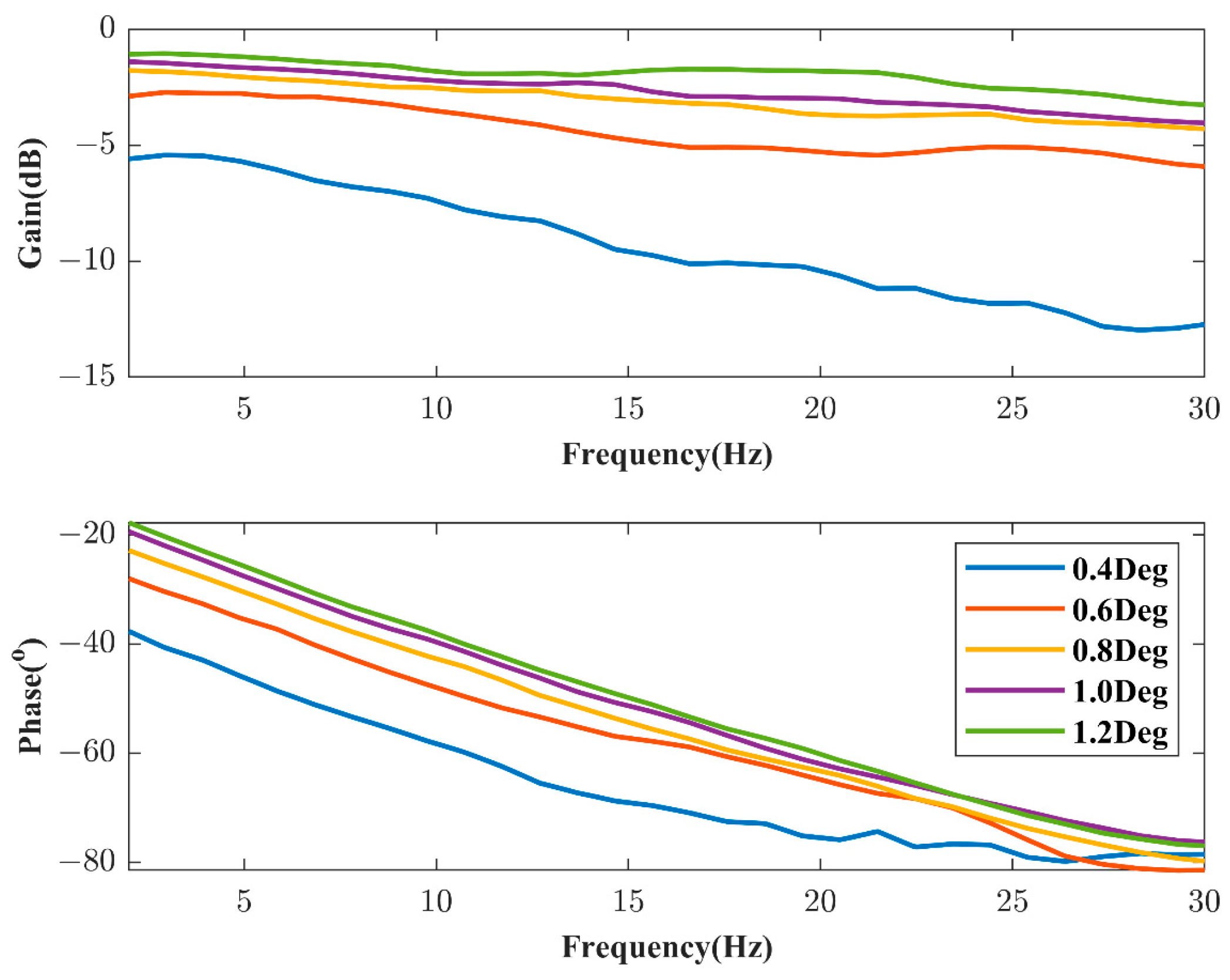
Generally, the frequency characteristics of the actuator under a command of around 1.0° better represent the real operational state of the control surface during airborne flight. Theoretical ASE analysis directly utilizes the obtained FRF of the actuator system from ground experiments, as illustrated in Figure 7. The FRF is identified using a step-sine signal with an amplitude of 1.0° as the deflection command. It is important to note that the actuator system in this paper is distinct from that presented in reference [15], which may impact the ASE stability analysis results.

3.1.3. Aerodynamic Derivative

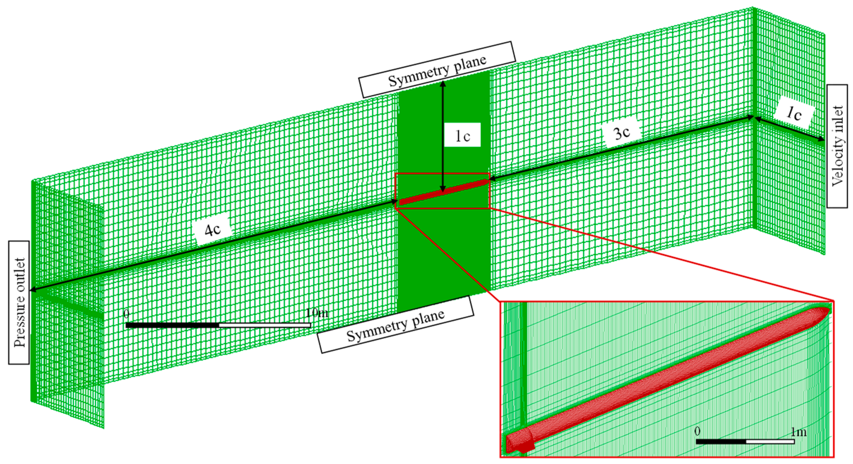
The quasi-steady aerodynamic derivative method is employed for the computation of aerodynamic forces. The body is segmented into 28 aerodynamic segments, with each control surface (right and left) treated as an independent segment, as illustrated in Figure 8. Utilizing a commercial CFD solver with the SST k-ω turbulence model and employing a second-order upwind scheme for numerical solving, the aerodynamic derivatives for each segment are computed. The structured mesh, which passes the grid independence test, is illustrated in Figure 9, where ‘c’ denotes the length of the slender vehicle and the total number of nodes is approximately 3.56 million. Considering sea level altitude and a Mach number of 0.5, the aerodynamic force acting on each segment is the resultant force from all its aerodynamic grids, with the projected areas of each segment in the X-Y plane serving as the segment’s area. The aerodynamic derivatives for each segment of the body are depicted in Figure 10, and the aerodynamic derivative for the control surface is 3.068/rad.

3.2. Experimental System Setup

The experimental setup for the GAT is depicted in Figure 11. The slender vehicle is subjected to a simulated free-free boundary using spring suspension. The aerodynamic force loading on the four excitation points is accomplished by two MB Dynamics Model 110 shakers and two Model 50A shakers. Four force sensors (Kisler 9712b250) are employed to capture the actual excitation forces. Eight acceleration sensors (PCB 333B30) are utilized to collect vibration accelerations at the measurement points, and integration is applied to derive the vibration velocities at these points. The vibration displacements at the measurement points are measured using eight laser displacement sensors (OPTEX CD5-150). The DPS comprises a National Instruments real-time PXIe module and a computer running a data processing program (coded in LabVIEW), with a working cycle of 0.5 ms. An embedded controller (PXIe-8840) is used for two-way communication between the host computer and the PXIe module. A PXI multifunction I/O module (PXI-6229) is used to collect the acceleration, displacement, and force signals. The PXI-6229 is also used to output the input voltages of the power amplifier.

The DPS is designed to perform three essential functions. (a) Real-time acquisition of signals from acceleration sensors, laser displacement sensors, and force sensors. Additionally, it integrates the acceleration signals to obtain velocity. (b) Computation of the condensed aerodynamic forces at each excitation point, based on the provided flight state and in accordance with Equation (4). (c) Execution of the force controller, generating the input voltage for each shaker power amplifier, and providing real-time output. These functionalities collectively enable the DPS to effectively manage the real-time data acquisition, aerodynamic force computation, and force control processes in the GAT.

The ground test procedure is outlined as follows:

(1) Set the flight state for conducting the ASE stability analysis. Activate the vehicle’s servo control system, including the IMU, FCS, and actuators.

(2) Activate the ACLS system. The DPS, based on collected vibration signals, flight state information, and aerodynamic derivatives, continuously computes the expected aerodynamic forces at each excitation point in real time. These forces are then transformed into input voltages for the power amplifiers through the force controller, subsequently driving the shakers.

(3) Incrementally increase the overall control gain ($k$) of the FCS until the observation of the ASE instability phenomenon. The corresponding control gain can be converted into the gain margin of the ASE system for the given flight state, based on the conversion to decibel units ($20\lg k$).

3.3. Partially Decoupled Approach to Force Control

In the experiment, we found that a partially decoupled approach can be employed to design the force controller based on the coupling strength between different shakers. This significantly simplifies the complexity of the force controller.

Taking the E1 shaker as an example, Figure 12 displays the FRFs obtained for the experiment, including G11, G12, G13, and G14. It can be observed that within the frequency range of 5 to 25 Hz, the amplitude of the FRFs for the input voltages of E2 and E3 to the actual force at E1 is below −20 dB. The amplitude of the FRF for the input voltage of E4 to the actual force at E1 is only slightly above −10 dB near the first bending mode, indicating a relatively larger coupling to point E1.

In accordance with Equation (14), the input voltages are also required to calculate the coupling strength coefficients between each shaker at different excitation points. In practical applications, a simpler yet viable approach can be adopted. Comparing the magnitudes of the input voltages for the four shakers is equivalent to comparing the magnitudes of the condensed aerodynamic forces at the ASE critical state for these points.

To calculate the aerodynamic forces at the four excitation points under the critical state, we employed Simulink to build a time-domain simulation model for the slender vehicle’s GAT system. Under the C2 flight control law, when the ASE critical state is reached, the ratio of condensed aerodynamic forces at the four points satisfies $f_{e1}:f_{e2}:f_{e3}:f_{e4}=1:-0.18:-0.13:42.3$. It can be approximated that the input voltages at these positions also follow this ratio. By calculating the coupling strength coefficients based on Equation (14), only ${\lambda }_{14}>0.1$. Therefore, it is required to consider the coupling from E4 to E1, and decoupling operations are needed. Figure 12 shows the fitted ${\tilde{G}}_{11}$ and ${\tilde{G}}_{14}$, which match well with the experimental results, meeting the requirements for force controller design. Similarly, decoupling controllers can be obtained for the other three shakers. The final design results in a partially decoupled force controller, as follows:

$$\begin{array}{l}{u}_1={\tilde{G}}_{11}^{-1}\left(f_{e1}-{\tilde{G}}_{14}{u}_4\right)\\ u_2={\tilde{G}}_{22}^{-1}\left(f_{e2}-{\tilde{G}}_{21}{u}_1-{\tilde{G}}_{24}{u}_4\right)\\ u_3={\tilde{G}}_{33}^{-1}\left(f_{e3}-{\tilde{G}}_{31}{u}_1-{\tilde{G}}_{34}{u}_4\right)\\ u_4={\tilde{G}}_{44}^{-1}{f}_{e4}\end{array}$$

(16)

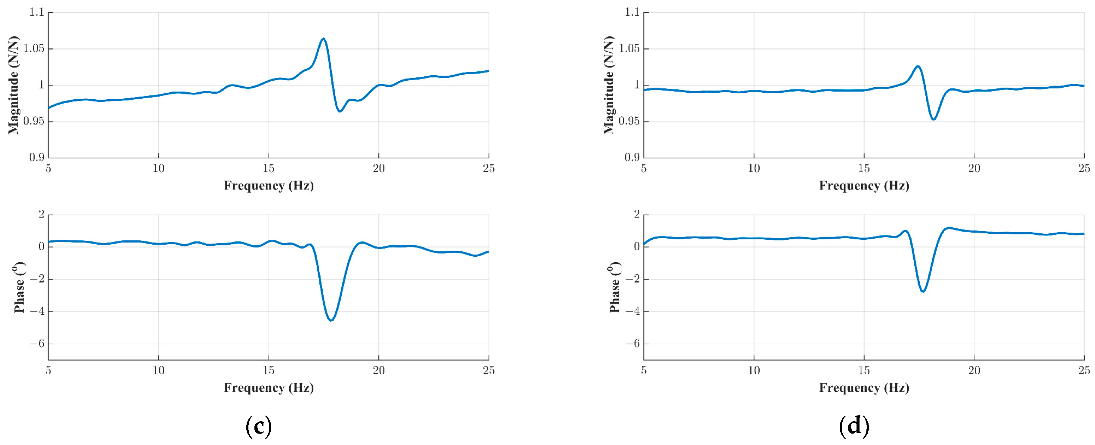
To validate the control effectiveness of the designed partially decoupled force controller, a linear sweep signal of expected force (${\mathit{f}}_e$) was simultaneously applied to all four excitation points. Referring to the magnitude relationship of aerodynamic forces at the four excitation points in the GAT, set the expected force amplitudes as follows: E1 with 2 N, E2 and E3 both with −0.2 N, and E4 with 80 N. With the force controller enabled, the identified FRFs of the expected force and the actual force are depicted in Figure 13. It can be observed that for points E1 and E4, the amplitude deviation between expected force and actual force does not exceed ±5%, and the phase error is within −3~1.5°. For points E2 and E3, the maximum amplitude error is less than ±10%, and the maximum phase error is within −7~1.5°. The maximum error occurs in the vicinity of the first bending mode frequency (18 Hz). Additionally, in other frequency ranges, both the amplitude and phase errors are extremely small. The force control results align with the conclusions of other researchers [18,19,20,21,22]; the closer to the elastic mode frequencies, the greater the force control error.

4. Results and Discussion

4.1. Influence of Excitation Force Amplitude and Phase Deviation

The precision of the force controller directly impacts the amplitude and phase deviation between the excitation force and the expected force. Strictly speaking, the magnitude of this deviation is related to the specific force controller, making it difficult to conduct quantitative studies. Therefore, we conduct research directly on the amplitude and phase deviation of the excitation force, leading to valuable conclusions.

The study on the impact of amplitude and phase deviation of the excitation force on GAT results is based on the time-domain simulation model depicted in Figure 14. It is assumed that the excitation force deviations at the four excitation points are consistent. The amplitude and phase of the condensed aerodynamic forces at each excitation point were fine-tuned to substitute for the control effects of the force controller. The adjustments in amplitude and phase were implemented through a gain, lead, and lag correction network, i.e., as follows:

$$\tau (s)=K\frac{1+aTs}{1+Ts}$$

(17)

where $K$ represents the gain coefficient, primarily employed to adjust amplitude characteristics. When $a>1$, it signifies a lead network, and when $a<1$, it indicates a lag network. $T$ denotes the time constant, and modifying the values of $a$ and $T$ is primarily used to adjust phase characteristics.

Under the C1 flight control law, appropriate parameters $K$, $a$, and $T$ were set to achieve specific deviations in excitation force amplitude at 10.8 Hz, namely 0%, ±5%, and ±10%, as well as phase deviations of 0° and ±5°. With an amplitude deviation of 0%, the network FRFs for various phase deviations are illustrated in Figure 15a. The results of time-domain simulation, including absolute error in gain margin and instability frequency, are listed in

Table 1. Absolute error of gain margin (C1 flight control law).

Amplitude Deviation	Phase Deviation
	−5°	0°	5°
−10%	1.06 dB	0.92 dB	0.68 dB
−5%	0.60 dB	0.45 dB	0.21 dB
0%	0.15 dB	0.00 dB	−0.23 dB
5%	−0.27 dB	−0.42 dB	−0.64 dB
10%	−0.67 dB	−0.82 dB	−1.04 dB

and

Table 2. Absolute error of instability frequency (C1 flight control law).

Amplitude Deviation	Phase Deviation
	−5°	0°	5°
−10%	−0.594 Hz	0.00 Hz	0.511 Hz
−5%	−0.589 Hz	0.00 Hz	0.513 Hz
0%	−0.585 Hz	0.00 Hz	0.515 Hz
5%	−0.580 Hz	0.00 Hz	0.517 Hz
10%	−0.575 Hz	0.00 Hz	0.519 Hz

. The absolute error in gain margin is within −1.04~1.06 dB, and the absolute error in instability frequency is within −0.60~0.52 Hz.

Under the C2 flight control law, adjustments were made to achieve specific deviations in excitation force amplitude and phase at 19.3 Hz. With an amplitude deviation of 0%, the network FRFs for various phase deviations are illustrated in Figure 15b. The results are listed in

Table 3. Absolute error of gain margin (C2 flight control law).

Amplitude Deviation	Phase Deviation
	−10°	−5°	−3°	0°	3°	5°	10°
−10%	−5.55 dB	−2.05 dB	−0.85 dB	0.92 dB	2.41 dB	3.35 dB	5.53 dB
−5%	−6.02 dB	−2.50 dB	−1.30 dB	0.45 dB	1.98 dB	2.92 dB	5.07 dB
0%	−6.42 dB	−2.95 dB	−1.70 dB	0.00 dB	1.57 dB	2.53 dB	4.63 dB
5%	−6.85 dB	−3.30 dB	−2.12 dB	−0.42 dB	1.16 dB	2.10 dB	4.23 dB
10%	−7.25 dB	−3.70 dB	−2.50 dB	−0.82 dB	0.78 dB	1.72 dB	3.85 dB

and

Table 4. Absolute error of instability frequency (C2 flight control law).

Amplitude Deviation	Phase Deviation
	−10°	−5°	−3°	0°	3°	5°	10°
−10%	−0.55 Hz	−0.30 Hz	−0.20 Hz	0.00 Hz	0.18 Hz	0.28 Hz	0.60 Hz
−5%	−0.55 Hz	−0.30 Hz	−0.18 Hz	0.00 Hz	0.18 Hz	0.30 Hz	0.62 Hz
0%	−0.53 Hz	−0.28 Hz	−0.18 Hz	0.00 Hz	0.20 Hz	0.30 Hz	0.62 Hz
5%	−0.53 Hz	−0.28 Hz	−0.18 Hz	0.00 Hz	0.20 Hz	0.32 Hz	0.65 Hz
10%	−0.50 Hz	−0.26 Hz	−0.16 Hz	0.00 Hz	0.20 Hz	0.32 Hz	0.65 Hz

. With a phase deviation within ±5°, the absolute error in gain margin is within −3.70~3.35 dB, and the absolute error in instability frequency is within −0.30~0.32 Hz. With a phase deviation increased to ±10°, the absolute error in gain margin is within −7.25~5.53 dB, and the absolute error in instability frequency is within −0.55~0.65 Hz.

Under the same phase deviation, the gain margin decreases during the process of amplitude deviation, ranging from −10% to 10% (i.e., the excitation force is 0.9 to 1.1 times the calculated condensed aerodynamic force). This aligns with theoretical expectations, indicating that if the excitation force is smaller, a higher overall control gain $k$ is required to induce instability in the ASE system, resulting in a higher gain margin.

In light of the characteristics of the slender vehicle’s ASE system, we discuss the simulation results. Observing the Bode plots of the open-loop FRFs under flight control laws C1 and C2, as depicted in Figure 16. The Bode plots around the vicinity of the instability frequency for both states are magnified and depicted in a single graph. The plots are redrawn with the instability frequency set to 0 Hz and the unwrap phase at the crossover frequency set to 0°. It can be observed that in the C1 state, the instability frequency is far from the first bending mode frequency, resulting in relatively flat magnitude and phase curves. Conversely, in the C2 state, the instability frequency is close to the first bending mode frequency, leading to a steep magnitude and phase curve. In the locally enlarged phase-frequency curve, the positions corresponding to a 5° phase lag (indicated by the black dashed line) and a 5° phase lead (indicated by the green dashed line) of the excitation force are marked. The corresponding positions on the gain-frequency curve are also indicated. A 5° phase lag corresponds to the original location, with a 5° phase angle in the phase-frequency curve becoming the new instability frequency point (phase angle 0°). It can be observed that the difference in slope causes a larger instability frequency error for the C1 state compared to the C2 state under the same excitation force phase deviation (±5°). However, C2 exhibits a larger absolute error in the gain margin.

For the C2 state, the impact of excitation force phase deviation on the stability margin of the ASE system is much greater than that of amplitude deviation. Due to the steep slope of the gain-frequency curve near the instability frequency, even a small phase deviation can result in a substantial deviation in the gain of the curve, significantly altering the gain margin. In fact, from the perspective of force controller precision, the accuracy of force control near the first bending mode frequency is also limited, as reflected in Figure 13. Therefore, in the GAT, it is advisable to maintain the amplitude and phase deviation of the excitation force within a specified range, with the simulation results for the C2 state being more indicative.

According to industry standards [34], for slender vehicles, a minimum gain margin of 6 dB, is required from a flight safety perspective. This necessitates that the error between the experimentally or theoretically derived gain margin and the actual gain margin should not exceed 6 dB. We believe that controlling this error within ±3 dB is appropriate. According to the simulation results for the C2 state, with excitation force amplitude deviation within ±10% and phase deviation within ±5°, the absolute error in gain margin ranges from −3.70 dB to 3.35 dB, basically meeting the accuracy requirements. Certainly, it would be optimal to control the phase deviation within ±3°, but achieving this may pose significant challenges for the force controller. Therefore, within the frequency range relevant to aeroelastic stability, we recommend controlling the excitation force amplitude deviation within ±10% and phase deviation within ±5° when using the GAT method.

4.2. GAT Results under Different Flight Control Laws

At a flight speed of 170 m/s and an atmospheric density of 1.225 kg/m³ (corresponding to a flight dynamic pressure of 17.7 kPa), the ground experiments were conducted for two sets of flight control laws, C1 and C2. When the vehicle was in a critical state, it exhibited near-harmonic vibration; however, accurately capturing this state in experiments proves challenging. Taking the example of the C2 state, the comparison between the expected and actual forces at E4 is illustrated in Figure 17. The excellent agreement between expected and actual forces verifies the effectiveness of the designed force controller.

In the case of the C2 flight control law, when the overall control gain was 26.44 dB, the ASE system remained stable, as depicted in Figure 17a, with aerodynamic forces quickly converging after the initial disturbance. As the overall control gain increased to 26.65 dB, the ASE system became unstable, as shown in Figure 17b, where aerodynamic forces gradually increased and diverged. In the experiments, the minimum control gain at which ASE instability was observed was identified as the gain margin for this flight state.

Comparisons between the experimental and theoretical results for the C1 and C2 control laws are summarized in

Table 5. Stability margin of the slender vehicle with different flight control laws.

State	Experimental Results		Theoretical Results
	Gain Margin (dB)	Instability Frequency (Hz)	Gain Margin (dB)	Instability Frequency (Hz)
C1	27.08	10.9	27.26	10.8
C2	26.65	19.1	27.31	19.3

. The experimental values closely align with the theoretical values. Due to the excellent force control precision of the designed force controller within the 5–25 Hz range, high-precision experimental results were obtained. The experimental error in the C2 state is slightly larger than that in the C1 state. This is attributed to the instability frequency of the ASE system in the C2 state being close to the first bending mode, where the force control precision is relatively lower. The experimental results further underscore the significance of maintaining excitation force amplitude deviations within ±10% and phase deviations within ±5°.

4.3. GAT Results at Different Dynamic Pressure

To verify the feasibility and accuracy of ground experiments under different flight dynamic pressures, under the C2 flight control law, the flight dynamic pressure varied from 17.7 kPa to 124.0 kPa. The comparison between experimental and theoretical results is illustrated in Figure 18. From the graph, it can be observed that within the dynamic pressure range below 70 kPa, experimental values closely align with theoretical values. However, as the flight dynamic pressure increases, the experimental gain margin gradually exceeds the theoretical values, and instability frequency errors also become larger. Despite varying flight dynamic pressures, the force controller operates reliably. However, the observed increase in errors with higher dynamic pressure prompts the question of why such discrepancies arise.

The occurrence of this phenomenon is attributed to the nonlinear characteristics of the actual actuator used in the experiment. Whether these nonlinear characteristics manifest is also related to the maximum output force capacity of the shaker. In this experiment, the maximum output force of the shaker is approximately 100 N. This means that the actual aerodynamic force output at each excitation point does not exceed 100 N. As shown in Figure 19, at a flight dynamic pressure of 93.2 kPa, the actual force at excitation point E4 is already below the expected force. With the limitation on aerodynamic forces, as the flight dynamic pressure increases, the deflection angle of the control surface will decrease. This causal relationship is easily deduced because, at the same control surface deflection angle, higher dynamic pressure results in larger aerodynamic forces. Conversely, under the same aerodynamic forces, higher dynamic pressure corresponds to a smaller control surface deflection angle. Taking the states of 17.7 kPa and 93.2 kPa as examples, the control surface deflection commands and return signals when the ASE system becomes unstable are illustrated in Figure 20. It can be observed that the former has a deflection command exceeding 1.5°, and the return signal indicates that the actual deflection angle closely matches the command. In contrast, the latter has a maximum deflection command of approximately 0.6°, and based on the return signal, the actual deflection angle is significantly smaller than the command. According to the measured FRFs of the actuator shown in Figure 21 and its relationship with the deflection command amplitude, as the deflection command amplitude decreases, both the amplitude and phase characteristics of the actuator deteriorate. This leads to the phenomenon observed in the experiment, where the gain margin exceeds the theoretical value.

It is noteworthy that, in numerical simulations, due to the linear transfer function model of the actuator, we did not observe this phenomenon. Specifically, the amplitude limitations on aerodynamic forces applied at the excitation point did not impact the accuracy of the ASE stability results. However, the actual actuator, influenced by nonlinear factors such as mechanical backlash, speed limitations, and amplitude constraints, exhibits nonlinear characteristics in its transfer function.

This experimental result underscores the importance of closely monitoring the excitation force amplitude and the deflection angle of the control surface in the experiments. If such nonlinear frequency response characteristics of the control surface exist, and the calculated expected force exceeds the shaker’s range, the experimental results may be less reliable. This can be addressed by selecting shakers with suitable ranges to improve experimental precision.

5. Conclusions

This paper presents a detailed exploration of the system composition, experimental methods, and experimental implementation of the GAT for slender vehicles, including the calculation and condensation methods for aerodynamics, the optimization of excitation and measurement points, and an improved inverse model force control method.

(1) Conducting ground experiments on a slender vehicle, a partially decoupled inverse model controller is designed based on the assessment of coupling strength between different shakers. The experiments indicate that, within the frequency range relevant to ASE stability, the force control precision is relatively high. The comparison with theoretical results verifies the accuracy of the GAT method under different flight control laws and flight dynamic pressures.

(2) The experimental results underscore the importance of closely monitoring the excitation force amplitude and control surface deflection angle in the experiments. Higher flight dynamic pressures require shakers with larger output capabilities, indirectly affecting control surface deflection angles and influencing the ASE stability margin in the experiment.

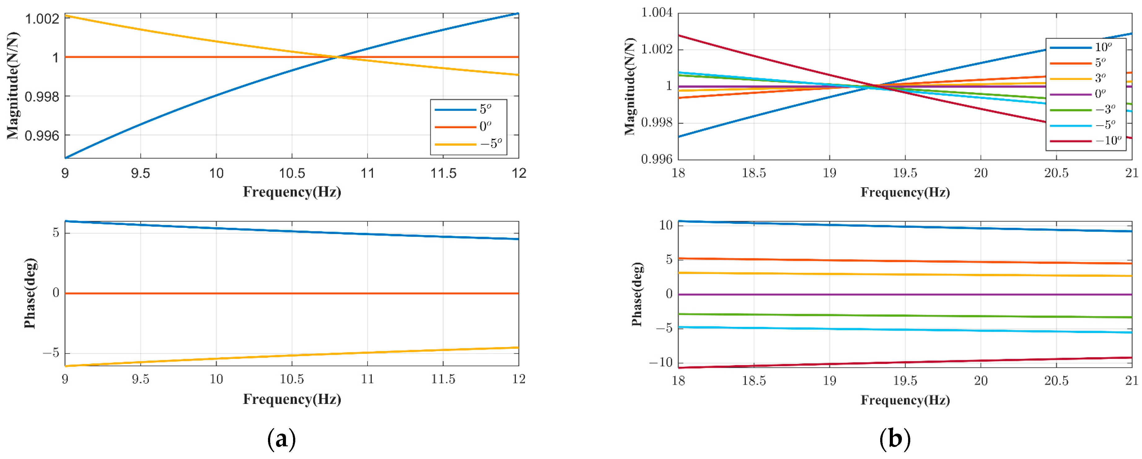
(3) Numerical simulations investigate the impact of excitation force amplitude and phase deviations on the ASE stability margin. We believe that an error in the gain margin of the ASE system within ±3 dB, as obtained from the method used, is reasonable. The experiments and numerical simulations indicate that, within the frequency range relevant to ASE stability, the designed force controller should ensure excitation force amplitude deviations are within ±10% and phase deviations are within ±5%.