Dual-Frequency Multi-Constellation Global Navigation Satellite System/Inertial Measurements Unit Tight Hybridization for Urban Air Mobility Applications

Abstract

A global navigation satellite system (GNSS) for remotely piloted aircraft systems (RPASs) positioning is essential, thanks to the worldwide availability and continuity of this technology in the provision of positioning services. This makes the GNSS technology a critical element as malfunctions impacting on the determination of the position, velocity and timing (PVT) solution could determine safety issues. Such an aspect is particularly challenging in urban air mobility (UAM) scenarios, where low satellite visibility, multipath, radio frequency interference and cyber threats can dangerously affect the PVT solution. So, to meet integrity requirements, GNSS receiver measurements are augmented/fused with other aircraft sensors that can supply position and/or velocity information on the aircraft without relying on any other satellite and/or ground infrastructures. In this framework, in this paper, the algorithms of a hybrid navigation unit (HNU) for UAM applications are detailed, implementing a tightly coupled sensor fusion between a dual-frequency multi-constellation GNSS receiver, an inertial measurements unit and the barometric altitude from an air data computer. The implemented navigation algorithm is integrated with autonomous fault detection and exclusion of GPS/Galileo/BeiDou satellites and the estimation of navigation solution integrity/accuracy (i.e., protection level and figures of merit). In-flight tests were performed to validate the HNU functionalities demonstrating its effectiveness in UAM scenarios even in the presence of cyber threats. In detail, the navigation solution, compared with a real-time kinematic GPS receiver used as the reference centimetre-level position sensor, demonstrated good accuracy, with position errors below 15 m horizontally and 10 m vertically under nominal conditions (i.e., urban scenarios characterized by satellite low visibility and multipath). It continued to provide a valid navigation solution even in the presence of off-nominal events, such as spoofing attacks. The cyber threats were correctly detected and excluded by the system through the indication of the valid/not valid satellite measurements. However, the results indicate a need for fine-tuning the EKF to improve the estimation of figures of merit and protection levels associated to the navigation solution during the cyber-attacks. In contrast, solution accuracy and integrity indicators are well estimated in nominal conditions.

1. Introduction

The use of a global navigation satellite system (GNSS) for drone positioning is essential, thanks to the worldwide availability and continuity of this technology in the provision of positioning services. The improvement in terms of accuracy of the consolidated constellations (i.e., the global positioning system, GPS), and the spatial and frequency diversity guaranteed by the new reliable and accurate constellations deployed (i.e., Galileo), make this technology even more promising and provide better performance. Moreover, the existing augmentation technologies allow high levels of accuracy and reliability to be reached; during the execution of beyond visual line of sight operations, GNSS (possibly augmented) is the preferred choice for navigation [1].

Drones often use GNSS for positioning purposes and an increasing number of manned commercial flights also use GNSS-based information.

GNSS will become soon the main means used by flight management systems (FMSs) for the navigation of the aircraft and, especially for the remotely piloted aircraft system (RPAS), it will be a critical element of the system, and malfunctions impacting on the determination of position, velocity and timing (PVT) solution should not be ignored [1].

It is certain that the use of multi-constellation and of new frequencies which are available in modern GNSS lead to the improved accuracy and availability of PVT. However, the main weakness of GNSS-based technologies is the lack of a simple, low-cost assessment of the level of positioning errors that affects the navigation system error (NSE), a relevant component of the overall total system error (TSE), which is strictly related to the determination of GNSS integrity [2] (pp. 103–130), [3].

The International Civil Aviation Organization (ICAO) in [4] lists the essential parameter specifications for radio navigation systems (including GNSS), which might aid the navigation of the aircraft. In the civil aviation domain, the navigation system guarantees the necessary level of safety giving in output the necessary levels of GNSS integrity in order to meet ICAO prescriptions in each flight phase. However, these standards cannot be directly applied to RPAS even if aviation standards are in the process of evolving to accommodate RPAS operations, and as such, the performance requirements are not yet formally specified for the use-cases that are foreseen in urban air mobility (UAM) scenarios [5,6].

Integrity requirements in civil aviation are met through a fault detection system that is either implemented onboard the mobile platform itself, or external to the mobile platform. The most common strategy is to employ a three-layered approach in assuring integrity. Differential corrections and integrity flags are provided to the user by satellite- and ground-based augmentation systems (SBASs/GBASs) which essentially rely on external reference receivers to monitor the positioning integrity and provide ‘do not use’ messages to the user when the estimated error exceeds the assigned limits [7]. The third augmentation layer is aircraft-based augmentation systems (ABASs) that augment/fuse GNSS receiver measurements with other aircraft sensors or signal of opportunities that are able to supply position and/or velocity information on the aircraft without relying on any other satellite and/or ground infrastructures (i.e., ABASs are independent of the other two layers) [8].

ABAS benefits are twofold. First, the use of onboard sensors and/or models is free of dependence on external reference receivers as in the case of SBASs and GBASs; second, user-level monitoring is necessary to protect against localized error sources such as multipath, which cannot be mitigated by differential techniques like SBASs or GBASs. For the listed reasons, ABASs assume primary importance over SBASs and GBASs in the urban environment even in rejecting cyber-attacks such as interferences impacting on GNSS bands (i.e., jamming) or manipulation of data presented to the receiver (i.e., spoofing attacks) [9].

Inertial navigation sensors (INSs) measure position by tracking the relative movements from a known initial position and represent an environment-independent and reliable source of information, guaranteeing continuity and availability in any challenging operation scenario. Even if they can provide an autonomous solution for the position and velocity (and attitude and heading), they suffer from drift over time. Coupled with absolute positioning systems, the drift error can periodically be reset to their location. Among all non-GNSS positioning technologies, inertial navigation occupies a special position, not only because it is ubiquitous, but also because it offers characteristics that make these two technologies naturally complement each other and ideal candidates for integration [10].

In [11], a review of GPS/INS hybridization and performance is provided. Here, the authors promote the benefits of using GPS with INS, as follows: integrated systems have higher accuracy; the additional information provided by the addition of sensors means more trust can be placed in the output, due to redundancy; the integrated output can be provided at a higher rate than GPS because of the higher data rate of INS; the integrated system will be available even during a GPS outage even if the time of availability is limited by the quality of the INS. This applies to both loosely and more tightly coupled systems [12]. However, [11] recommends tightly coupled methods that even with less than four satellites in view could maintain the navigation solution. Furthermore, the access to the pseudo-range measurements can provide the benefit of slowly detecting growing errors. A stated disadvantage is that tightly coupled systems respond more slowly to INS errors than loosely coupled systems. Based on GPS/INS hybridization algorithms and considering that the INS is fault-free, different sequential detection approaches have been investigated in the literature. Two are the most popular works. The first method is the autonomous integrity monitoring extrapolation (AIME) method [13]. This method was devised to detect slowly growing errors by observing the GPS measurements over a relatively long period (up to 30 min) for an en-route and non-precision approach (0.3 nm accuracy limit) phase of flight, even with three satellite failures in the constellation [14].

The second one is the multiple hypothesis solution separation (MHSS). The MHSS method [15] is an extension of the classical snapshot solution separation receiver autonomous integrity monitoring (RAIM) concept [16] applied to a GPS/inertial system. In this method, a full Kalman filter (i.e., that uses all the available satellite measurement) is used together with a set of separate sub-Kalman filters, one for each satellite. A sub-filter and a covariance propagator are assigned to each tracked satellite in order to rigorously incorporate the basic fault detection requirements (i.e., single failure assumption).

Ensuring integrity for GNSS/INS systems is fundamental to achieve higher performance levels for future dual-frequency, multi-constellation [17] aviation services and is of vital importance for new ground and air applications like autonomous vehicles or urban air mobility.

Another advantage of inertial hybridization of GNSS is the possibility of using inertial aid to detect spoofing attacks. In recent works, Kalman filter-based INS monitors for GNSS spoofing detection are proposed for both tightly and loosely coupled INS/GNSS systems. In [18], a cumulative test statistic defined as the sum of weighted norm of the innovation vectors is used for spoofing detection. Meanwhile, in [19], the fault detection test statistic is constructed with the sum of squares of the residuals weighted by the measurement variance–covariance matrix. In these works, the innovation- or residual-based spoofing detection algorithms have shown their effectiveness in spoofing detection. Some spoofing detection ability of off-the-shelf aviation-grade INS/GNSS systems (based on solution separation or AIME) has been proved without any additional changes or supplements [20].

A specific minimum operational performance standards (MOPSs), is completely dedicated to the hybridization of GNSS and inertial system considering different classes of precision spanning from navigation grade to tactical grade systems [21]. This MOPS focuses on the integrity, continuity, and availability requirements for GPS/INS.

In this framework, in this paper, the algorithms are detailed of a hybrid navigation unit (HNU) for UAM applications implementing a tightly coupled sensor fusion between a dual-frequency multi-constellation (DFMC) GNSS receiver (in standalone configuration), an inertial measurements unit (IMU with closed-loop fibre optic gyroscope technology and quartz accelerometer) and barometric altitude from an air data computer (ADC). The implemented navigation algorithm is integrated together with autonomous fault detection and exclusion (FDE) of GPS/Galileo/BeiDou satellites and estimation of the navigation solution integrity/accuracy (in terms of protection level and figures of merit). The HNU has been verified through fast-time and real-time simulations and then validated by means of in-flight tests performed deploying the HNU on a real-time hardware and embarking it on an RPAS. Details of the implemented algorithms, in-flight test rig set-up and related results will be described in the paper.

In the next section, the functional architecture of the HNU will be described detailing the navigation and the fault detection and exclusion algorithms implemented. In section three, the validation test rig and the in-flight test results will be reported. Finally, the conclusions and further works will be given in the fourth section.

2. The Hybrid Navigation Unit System

The HNU system implements all the algorithms for a tightly coupled sensor fusion between a DFMC GNSS receiver (in standalone configuration), an IMU (with closed-loop fibre optic gyroscope technology and quartz accelerometer) and barometric altitude from an ADC, together with related autonomous FDE and integrity monitoring algorithms.

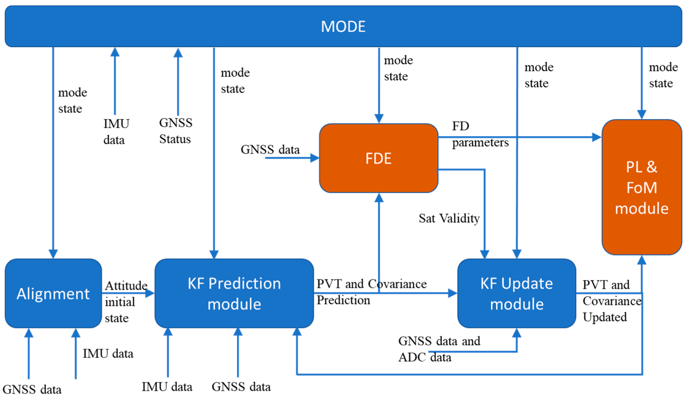
Figure 1 shows the functional architecture of the system.

The Alignment module estimates the initial attitude state of the system in terms of roll, pitch and true heading angles through the IMU measurements in input. The module starts the alignment process when it is powered on and continues for a specified alignment time, which can be adjusted based on the desired accuracy. The first step in the alignment process is the calculation of the mean values of the IMU measurements. This is achieved by collecting and averaging the IMU measurements over a specified time. Once the mean values of the IMU measurements have been calculated, the Alignment module uses a combination of levelling and gyro compassing to estimate the orientation of the system [22,23]. On the other side, the Mode module implements the logic to allow all the HNU’s elements to correctly initialize and evolve. In detail, taking advantage of the IMU measurements the Mode module verifies that the vehicle is in static conditions, i.e., the measured accelerations and angular velocities are below appropriate thresholds, for all the duration of the coarse alignment process. If a movement is detected, the module changes its state in motion detection during which the acquired samples are not used for the alignment process. At the end of the coarse alignment, the Mode state goes into a zero-velocity update (ZUPT) state during which a fine alignment process of the extended Kalman filter (EKF) is activated in static conditions with zero velocity measurements forced into input. After five minutes, the ZUPT operative state is activated. In this state, the HNU is completely initialized and also ready to dynamically estimate the aircraft state. Indeed, an extended Kalman filter integrated with the FDE module, determining the valid satellite measurements, computes the navigation solution in terms of estimated position, velocity, attitude and related covariance, while a dedicated module provides the protection level (PL) and the figure of merit (FoM) of the solution.

Details of the implemented algorithms are given in the next sections.

2.1. Kalman Filter Prediction Module

The objective of the EKF module of the HNU is to provide a complete navigation solution by estimating the orientation and the position of the system in real-time. The EKF uses measurements from a multi-constellation GNSS receiver and an IMU to achieve this goal. Three constellations are used by the Kalman filter, GPS, Galileo and BeiDou. The implemented EKF algorithm is error state and closed loop; at each iteration of the algorithm, when an update happens, the error state is reset. Its computational complexity, as reported in [24], scales as the cube of the dimension of the state vector defined in (1).

In the KF prediction module, the state estimate and the state covariance matrix are updated based on process model, which predicts the future state of the system based on the current state and the dynamic model [2] (pp. 382–424). The module has as inputs the last estimate and the state covariance and last IMU measurements and outputs the predicted state and the predicted covariance matrix.

The Kalman filter has nineteen states, as reported below:

$$\overline{\mathit{x}}={\left[\overline{\mathit{\phi }},\mathit{\delta }{\overline{\mathit{v}}}^n,\mathit{\delta }\overline{\mathit{p}},{{\overline{\mathit{\epsilon }}}^b,{\overline{\mathit{𝛻}}}^{\mathit{b}},\overline{\mathit{x}}}_{\mathit{C}\mathit{l}\mathit{o}\mathit{c}\mathit{k}}\right]}^{\mathit{T}}\in {\mathit{R}}^{19},$$

(1)

where $\overline{\mathit{\phi }}$ is the mathematical platform misalignment angles array; $\mathit{\delta }{\overline{\mathit{v}}}^n$ is the velocity errors array; $\mathit{\delta }\overline{\mathit{p}}$ is the position errors array in terms of latitude, longitude and altitude; ${\overline{\mathit{\epsilon }}}^b$ is the gyros drift error array expressed in body frame; ${\overline{\mathit{𝛻}}}^{\mathit{b}}$ is the accelerometer errors array expressed in body frame; and ${\overline{\mathit{x}}}_{\mathit{C}\mathit{l}\mathit{o}\mathit{c}\mathit{k}}$ is the clock state array composed of ${dt}_G$ GPS receiver clock offset; ${dt}_{GE}$ Galileo receiver clock offset w.r.t GPS; ${dt}_{GC}$ BeiDou receiver clock offset w.r.t GPS; ${dt}_d$ GPS receiver clock drift.

Once defined, the key initial states related to position, velocity and attitude, derived from the GNSS and the alignment module, the EKF prediction is executed in two steps. First, the states are integrated using the process equations to provide a predicted state and then the predicted covariance matrix is computed.

The state inertial integration can be divided in three steps (see Figure 2):

• attitude update:

  $${\stackrel{̿}{\mathit{C}}}_{b_k}^{n_k}={\stackrel{̿}{\mathit{C}}}_{n_{k-1}}^{n_k}{\stackrel{̿}{\mathit{C}}}_{b_{k-1}}^{n_{k-1}}{\stackrel{̿}{\mathit{C}}}_{b_k}^{b_{k-1}}$$

  (2)

  where ${\stackrel{̿}{\mathit{C}}}_{b_k}^{b_{k-1}}$ is rotation matrix from body frame at time $t_{k-1}$ to body frame at $t_k$ derived from ${\overline{\mathit{\omega }}}_{ib}^b$ [25] including coning correction [26]. ${\stackrel{̿}{\mathit{C}}}_{b_{k-1}}^{n_{k-1}}$ is the body frame to navigation frame rotation matrix at time $t_{k-1}$. ${\stackrel{̿}{\mathit{C}}}_{n_k}^{n_{k-1}}$ is the rotation matrix from navigation frame at time $t_{k-1}$ to navigation frame at $t_k$ derived from ${\overline{\mathit{\omega }}}_{in}^n$ [25].
• velocity update, also implementing the coning and sculling correction [27]:

  $${\overline{\mathit{v}}}_{\mathit{k}}^{\mathit{n}}={\overline{\mathit{v}}}_{\mathit{k}-1}^{\mathit{n}}+∆{\overline{\mathit{v}}}_k^n$$

  (3)

  where $∆{\overline{\mathit{v}}}_k^n$ is computed from $∆{\mathit{v}}_{sf}^b$ (accelerometer measurements) and sculling correction [25].
• position update:

$${\overline{\mathit{p}}}_k={\overline{\mathit{p}}}_{k-1}+{\stackrel{̿}{\mathit{M}}}_{pv}{\displaystyle \frac{{\overline{\mathit{v}}}_{\mathit{k}}^{\mathit{n}}+{\overline{\mathit{v}}}_{\mathit{k}-1}^{\mathit{n}}}{2}}DT$$

(4)

$${\stackrel{̿}{\mathit{M}}}_{pv}=\left[\begin{array}{ccc}0& {\displaystyle \frac{1}{R_M+h}}& 0\\ {\displaystyle \frac{\mathrm{s}\mathrm{e}\mathrm{c}\left(L\right)}{R_N+h}}& 0& 0\\ 0& 0& 1\end{array}\right]$$

(5)

where $R_M$ and $R_N$ are the meridian and transverse radii of the curvature of the Earth computed at latitude $L$, respectively.

In order to compute the predicted covariance, with DT representing the Kalman filter time step, Q the process noise matrix and G the system noise distribution matrix, KF prediction is computed with the following equations:

$${\stackrel{̿}{\mathit{Q}}}_{\mathit{z}}=\stackrel{̿}{\mathit{G}}\stackrel{̿}{\mathit{Q}}{\stackrel{̿}{\mathit{G}}}^{\mathit{T}}\ast DT$$

(6)

$${\stackrel{̿}{\mathit{P}}}_{\mathit{z}}=\stackrel{̿}{\mathit{P}}+{\displaystyle \frac{1}{2}}\stackrel{̿}{\mathit{Q}}$$

(7)

$$\stackrel{̿}{\mathit{P}}=\stackrel{̿}{\mathit{\Phi }}{\stackrel{̿}{\mathit{P}}}_{\mathit{z}}{\stackrel{̿}{\mathit{\Phi }}}^{\mathit{T}}+{\displaystyle \frac{1}{2}}{\stackrel{̿}{\mathit{Q}}}_{\mathit{z}}$$

(8)

where $\mathit{\Phi }$ in (4) is the state transition matrix and is computed by linearization of the dynamic matrix $\stackrel{̿}{\mathit{F}}$:

$$\stackrel{̿}{\mathit{\Phi }}={\stackrel{̿}{\mathit{I}}}_{19\mathit{x}19}+\stackrel{̿}{\mathit{F}}\ast DT$$

(9)

with $\stackrel{̿}{\mathit{F}}$ computed as follows:

$$\stackrel{̿}{\mathit{F}}=\left[\begin{array}{cc}{\stackrel{̿}{\mathit{F}}}_{\mathit{I}\mathit{N}\mathit{S}}& {\stackrel{̿}{0}}_{15\times 4}\\ {\stackrel{̿}{0}}_{4\times 15}& {\stackrel{̿}{\mathit{F}}}_{\mathit{C}\mathit{l}\mathit{o}\mathit{c}\mathit{k}}\end{array}\right]$$

(10)

$${\stackrel{̿}{\mathit{F}}}_{\mathit{C}\mathit{l}\mathit{o}\mathit{c}\mathit{k}}=\left[\begin{array}{cccc}0& 0& 0& DT\\ 0& 0& 0& 0\\ 0& 0& 0& 0\\ 0& 0& 0& 0\end{array}\right]$$

(11)

$${\stackrel{̿}{\mathit{F}}}_{INS}=\left[\begin{array}{ccccc}{\stackrel{̿}{\mathit{M}}}_{aa}& {\stackrel{̿}{\mathit{M}}}_{av}& {\stackrel{̿}{\mathit{M}}}_{ap}& -{\stackrel{̿}{\mathit{C}}}_b^n& {\stackrel{̿}{0}}_{3\times 3}\\ {\stackrel{̿}{\mathit{M}}}_{va}& {\stackrel{̿}{\mathit{M}}}_{vv}& {\stackrel{̿}{\mathit{M}}}_{vp}& {\stackrel{̿}{0}}_{3\times 3}& {\stackrel{̿}{\mathit{C}}}_b^n\\ 0_{3\times 3}& {\stackrel{̿}{\mathit{M}}}_{pv}& {\stackrel{̿}{\mathit{M}}}_{pp}& {\stackrel{̿}{0}}_{3\times 3}& {\stackrel{̿}{0}}_{3\times 3}\\ {\stackrel{̿}{0}}_{3\times 3}& {\stackrel{̿}{0}}_{3\times 3}& {\stackrel{̿}{0}}_{3\times 3}& {\stackrel{̿}{\mathbf{I}}}_{3\times 3}\ast \left({\displaystyle \frac{1}{ta{u}_g}}\right)& {\stackrel{̿}{0}}_{3\times 3}\\ {\stackrel{̿}{0}}_{3\times 3}& {\stackrel{̿}{0}}_{3\times 3}& {\stackrel{̿}{0}}_{3\times 3}& {\stackrel{̿}{0}}_{3\times 3}& {\stackrel{̿}{\mathbf{I}}}_{3\times 3}\ast \left({\displaystyle \frac{1}{ta{u}_a}}\right)\end{array}\right]$$

(12)

where ${\tau }_g$ and ${\tau }_a$ are the correlation times of the gyroscopes and accelerometers biases, respectively.

The dependencies of ${\stackrel{̿}{\mathit{M}}}_{ii}$ are available in references such as [25,28].

2.2. Fault Detection and Exclusion

This module provides an enhanced GNSS satellite FDE with respect to conventional RAIM when using civil GPS. Improved performances are obtained by combining an FDE algorithm that uses tightly coupled KF process updates (AIM FDE) with a snapshot FDE algorithm based on an extended RAIM algorithm (ERAIM FDE) that can be applied to multi-constellation measurements, with no assumption of the prior satellite failure probability and satellite error modelling (like ARAIM [25,29]).

The use of a snapshot algorithm offers two key advantages. First, it relies solely on current measurements and satellite data, enabling the real-time execution of the algorithm characterized by a lower computational complexity with respect to recursive algorithms. Additionally, it can effectively identify and slowly exclude increasing satellite measurement errors. Moreover, the combination of the ERAIM FDE with the results of AIM FDE allows some types of simple cyber-attacks to be detected. Indeed, a highly probable spoofing attack is considered when AIM FDE excludes all the satellites from a constellation while the ERAIM FDE does not. This event is indicated by a dedicated code in the FDE output, while the spoofing attack is automatically mitigated as none of the spoofed GNSS satellites are used in computing the hybrid navigation solution by the Kalman filter.

The final results of the FDE module are the set of validated satellite measurements that can be used by the EKF update step algorithm and a set of information that are used for finally computing the fused PLs and FoM, by the respective software modules.

2.2.1. AIM FDE

The AIM FDE module performs failure detection using a chi-square failure detection test based on KF-predicted residuals and, in case of a failure detection, performs exclusion by checking the validity of each GNSS satellite. Actually, any measurement that is not aligned with the estimation provided by the current EKF prediction state is excluded and, therefore, also satellites that could have been affected by heavy multipaths would be detected and excluded. The algorithm is a measurement coherence test and it is based on the procedure described in [30] (Sections 3.1.1 and 3.2).

The steps of the AIM FDE are as follows:

• Perform conversion of the EKF state and covariance prediction from the latitude, longitude, altitude (LLH) reference coordinates to Earth-centred Earth-fixed (ECEF), which is the reference frame of the AIM FDE algorithm. This is accomplished using the reference and covariance relations described in [31];
• Compute mean sea level values for referencing the barometric altitude taking advantage of an earth gravity model like the Earth Geopotential Model (EGM96) easily available from open source;
• Detect possible failures of the satellites using the EKF predictions;
• In case of failure detection, attempt exclusion.

The algorithm for failure detection sets a fail detected integer (FD) for each constellation that indicates some satellite failure, using a chi-square test based on predicted residual, as described in [30] (Section 3.1.1).

The first step is to compute virtual pseudo-ranges ${\rho }_{v_{i_k}}$ from INS data and GNSS satellite measurements. This comes out from the standard equation of GNSS ranging satellites. For all indexes i of the valid constellation satellites:

$${\rho }_{v_{i_k}}=\sqrt{{\left(x_{S_i}-{\widehat{x}}_{k,k.1}\right)}^2+{\left(y_{S_i}-{\widehat{y}}_{k,k.1}\right)}^2+{\left(z_{S_i}-{\widehat{z}}_{k,k.1}\right)}^2}+c·{\tau }_{k,k-1}$$

(13)

where ${{\overline{\mathit{P}}}_S}_i=(x_{S_i}, y_{S_i},z_{S_i})$ is the satellite position in ECEF; ${\left(\widehat{{\mathit{P}}_{RX}},\widehat{\tau }\right)}_{k,k-1}$ is the predicted position from EKF and the constellation related clock offset; and c is the speed of light.

Then, a partial output measurement matrix should be computed (i.e., the linear satellite observability matrix). This is the matrix $\stackrel{̿}{{\mathit{H}}_k}$ having dimension NSATx4, where NSAT is the number of the specific constellation satellites in view, with each row i computed as follows:

$${\stackrel{̿}{\mathit{H}}}_{i_k}=\left[{\displaystyle \frac{{\left({\overline{\mathit{P}}}_{S_i}-{\overline{\mathit{P}}}_{{RX}_{k,k-1}}\right)}^T}{‖\left({\overline{\mathit{P}}}_{S_i}-{\overline{\mathit{P}}}_{{RX}_{k,k-1}}\right)‖}}\right]$$

(14)

Then, we define the measurement covariance matrix $\stackrel{̿}{{\mathit{R}}_k}$:

$$\stackrel{̿}{{\mathit{R}}_k}=\left[\begin{array}{ccc}{\sigma }_{{UERE}_1}^2& \cdots & 0\\ ⋮& \ddots & ⋮\\ 0& \cdots & {\sigma }_{{UERE}_{NSAT}}^2\end{array}\right]$$

(15)

Therefore, we can now compute the predicted residual error of dimension NSAT for each satellite constellation:

$${\overline{\mathit{\upsilon }}}_k=\left({\overline{\mathit{\rho }}}_{v_k}-{\overline{\mathit{\rho }}}_{{SAT}_k}\right)-\stackrel{̿}{{\mathit{H}}_k}·{\left(\widehat{{∆\mathit{P}}_{RX}},\widehat{∆\tau }\right)}_{k,k-1}$$

(16)

and its covariance:

$${\stackrel{̿}{\mathit{C}\mathit{o}\mathit{v}}}_{{\overline{\mathit{\upsilon }}}_k}={\stackrel{̿}{\mathit{H}}}_k·{\stackrel{̿}{\mathit{C}\mathit{o}\mathit{v}}}_{k,k-1}·{\stackrel{̿}{\mathit{H}}}_k^T+{\stackrel{̿}{\mathit{R}}}_k.$$

(17)

And finally compute the test statistics below:

$${\mathsf{\Lambda }}_k={\overline{\mathit{\upsilon }}}_k^T·{\stackrel{̿}{\mathit{C}\mathit{o}\mathit{v}}}_{{\overline{\upsilon }}_k}^{-1}·{\overline{\mathit{\upsilon }}}_k$$

(18)

${\mathsf{\Lambda }}_k$ is a scalar stochastic process that has a chi-squared distribution with NSAT degree of freedom. Therefore, we can define the test statistic threshold T_D with a given probability of false alarm P_FA, as follows:

$$T_D={\chi }_2^{-1}\left(NSAT,P_{FA}\right)$$

(19)

where ${\chi }_2^{-1}\left(NSAT,P_{FA}\right)$ is the tabled inverse of the chi-square cumulative distribution function of order NSAT, with NSAT being the total number of real satellites under consideration with related covariances.

So, a fault is declared (FD = 1), as follows:

$$FD=\left\{\begin{array}{c}1 if {\mathsf{\Lambda }}_k>T_D\\ 0 if {\mathsf{\Lambda }}_k\le T_D\end{array}\right.$$

(20)

In case of a failure detection (FD = 1), the AIM FDE failure exclusion functionality identifies failed satellites using a method similar to that described in [30] (Section 3.2).

This algorithm sets the validity data of the GNSS satellites as follows: equal to 0 if the satellite is not in view or it is declared failed; equal to 1 if it is a valid measured pseudo-range.

First, it computes the false alert probability for each satellite by deriving it from P_FA:

$$P_{FA0}=1-\sqrt[NSAT]{1-P_{FA}}$$

(21)

If a failure has been detected by the above algorithm (denoted as global test) then, for each valid satellite i of each constellation, the following sequence of operations is executed:

• Compute the standardized residual for each satellite at epoch k:

  $${\lambda }_k^i={\displaystyle \frac{{\overline{\mathit{c}}}_i^T·{\stackrel{̿}{\mathit{C}\mathit{o}\mathit{v}}}_{{\overline{\mathit{\upsilon }}}_k}^{-1}·{\overline{\mathit{\upsilon }}}_k}{\sqrt{{\overline{\mathit{c}}}_i^T·{\stackrel{̿}{\mathit{C}\mathit{o}\mathit{v}}}_{{\overline{\mathit{\upsilon }}}_k}^{-1}·{\overline{\mathit{c}}}_i}}}$$

  (22)

  where ${\overline{\mathit{c}}}_i$ is a vector with NSAT elements of 0 and 1 only in the i-th position;
• Compute the value of ${\lambda }_{Max}=\mathrm{m}\mathrm{a}\mathrm{x}\left({\lambda }_k^i\right)$;
• Update the element VAL_i as follows:

  $${VAL}_i=\left\{\begin{array}{c}0 if \left|{\lambda }_k^i\right|>N_{P_{FA0}/2}\left(\mathrm{0,1}\right)\\ 1 if \left|{\lambda }_k^i\right|\le N_{P_{FA0}/2}\left(\mathrm{0,1}\right)\end{array}\right.$$

  (23)

  where $N_{P_{FA0}/2}\left(\mathrm{0,1}\right)$ is the value that corresponds to a P_FA0/2 probability for a normal distribution having 0 mean and a standard deviation of 1;
• If more than one of above tests have failed, then remove only the satellite that has ${\lambda }_{Max}$ and repeat the global test (that is now more a sanity check) on the remaining satellites;
• Exit only if the global test is successful; otherwise, repeat steps from 1 to 4.

The final output of this algorithm will produce the new VAL_i array that informs which of ${\left(\rho ,{\sigma }_{UERE}\right)}_i$ are valid.

Moreover, if a failure has been detected but not one of the tests of the previous equation has identified at least a failed satellite, then the failure-detected flag FD shall be set to 2, meaning that the algorithm has been not able to identify a satellite to be excluded.

2.2.2. ERAIM FDE

This module implements an extended FDE/RAIM algorithm in which the GPS solution and satellites are first validated and then the satellites of the other constellations are validated using results from the pseudo-range (PR) pre-screening module. This algorithm is derived from a technique used for the integration of GPS receiver measurements with an IMU unit considering a tight-coupled fusion [30].

This strategy allows minimal assumptions and knowledge of the Galileo and BeiDou constellations while exploiting the heritage of several years of GPS usage in terms of reliability. The only assumption here is that GPS can have only a single failure (after the AIM FDE module) and that any satellite failure on a GPS constellation is not correlated with Galileo and BeiDou failures that conversely may also have multiple simultaneous satellite failures (any number). On the other hand, navigation integrity can only be assessed when the GPS solution is validated (e.g., when the number of satellites is above 5), preventing the use of GPS in low visibility conditions, even if the total number of satellites considering also the other constellations is well above the minimum number of satellites.

First, as with AIM FDE, this module shall be executed at each new measurement from the GNSS receiver and when a valid solution from the EKF is available, to avoid unnecessary computations.

The following steps are performed by the ERAIM algorithm:

• Apply the appropriate masking angle to the current ranging satellites above the horizon that are valid, using the position of the receiver at the preceding epoch. The mask angle is typically 2 deg for en-route and imprecise operations and 5 deg for precision operations;
• Compute the total sigma accuracy of residual errors for GPS satellites using the procedure [32] (Appendix J), in case of single-frequency, and [33] for multi-frequency. The expressions of the various sigma components in both cases are computed using the elevation and azimuth of ranging satellites estimated using the last valid ERAIM computed position. For L1 mode:

  $${\sigma }_{i,SPS}^2={\sigma }_{i,tropo}^2+{\sigma }_{i,URA}^2+{\sigma }_{i,air}^2$$

  (24)

  For L1/L5 mode:

  $${\sigma }_{i,DF}^2={\sigma }_{i,tropo}^2+{\sigma }_{i,DFC}^2+{\sigma }_{i,airDF}^2$$

  (25)

  The terms in (24) and (25) express the covariance of each residual error correction after GNSS receiver compensations have been applied. Specifically, the subscripts DF stands for dual-frequency, tropo for tropospheric, iono for ionospheric (residual error after single or double frequency compensation is applied), air for RF receiver and multipath errors, URA for user range accuracy and DFC for the residual error after dual-frequency compensation.
• Compute the full in view position and velocity fix using only the GPS satellites. The position fix is computed using an iterative weighted least mean squares algorithm with weights given by the sigmas computed at step 1, according to [32] (Appendix E). The unknowns are given by the position and clock offset of the receiver. Specifically, the following linear algebraic system equation is solved, as follows:

  $$\overline{∆\mathit{\rho }}=\stackrel{̿}{\mathit{G}}·{\left(\overline{∆\mathit{P}}, c\tau \right)}^T+\overline{\mathit{\epsilon }}$$

  (26)

  where $\overline{∆\rho }$, $\overline{∆P}$ and $c\tau$ are the PR errors, the position errors and the clock offset, respectively, and $\stackrel{̿}{G}$ is the observability matrix:

  $${\overline{\mathit{G}}}_i=\left[\begin{array}{cc}{\displaystyle \frac{{\left({\overline{\mathit{P}}}_{S_i}-{\overline{\mathit{P}}}_{k-1}\right)}^T}{‖\left({\overline{\mathit{P}}}_{S_i}-{\overline{\mathit{P}}}_{k-1}\right)‖}}& +1\end{array}\right]$$

  (27)

  where ${\overline{\mathit{P}}}_{S_i}$ are the GPS satellite positions and ${\overline{\mathit{P}}}_{k-1}$ are the estimated positions at the previous iteration. The weighted least mean squares solution of the above system equation is found by iteration using the following tentative solutions until the position errors are below a given threshold:

  $${\left(\overline{∆\mathit{P}}, c\tau \right)}^T=\stackrel{̿}{\mathit{S}}·\overline{∆\mathit{\rho }}, \stackrel{̿}{\mathit{S}}={\left({\stackrel{̿}{\mathit{G}}}^T\stackrel{̿}{\mathit{W}}\stackrel{̿}{\mathit{G}}\right)}^{-1}{\stackrel{̿}{\mathit{G}}}^T\stackrel{̿}{\mathit{W}}$$

  (28)

  where $\stackrel{̿}{\mathit{W}}=diag\left({\displaystyle \frac{1}{{\sigma }_i^2}}\right)$ is the weight matrix of the measured PR.
  The velocity fix can be found using an algorithm similar to the above step, as reported in [32] (Appendix F).
• Perform FDE on GPS satellites using standard RAIM algorithms (any standard RAIM is equivalent as specified in [32]). Here, we adopted an algorithm that implements a Least Square Residuals method for failure detection and a Solution Separation method for excluding a failed GPS satellite. Specifically, the following is performed:
  Compute the residuals w and test statistics T:

  $$T=\sqrt{{\overline{\mathit{w}}}^T\stackrel{̿}{\mathit{W}}\overline{\mathit{w}}}, \mathit{w}=\stackrel{̿}{\mathit{A}}·\left(\overline{\mathit{\rho }}-\stackrel{̿}{\mathit{G}}·{\left(\widehat{\mathit{P}},\widehat{\mathit{b}}\right)}^T\right), \stackrel{̿}{\mathit{A}}=\left(\stackrel{̿}{\mathit{I}}-\stackrel{̿}{\mathit{G}}·\stackrel{̿}{\mathit{S}}\right)$$

  (29)

  The failure is declared as in the following standard least square residuals RAIM method:

  $$\mathrm{F}\mathrm{a}\mathrm{i}\mathrm{l}\mathrm{u}\mathrm{r}\mathrm{e} \mathrm{i}\mathrm{f} T>\sqrt{T_P}, T_P={\chi }_2^{-1}\left(NSAT,P_{FA}\right)$$

  (30)

  where ${\chi }_2^{-1}\left(NSAT,P_{FA}\right)$ is the tabled inverse of the chi-square cumulative distribution function of order (N − 4), with NSAT being the total number of GPS satellites under consideration [32] with related covariances.
  When a failure is declared, the failure detection described in the above step shall be executed by removing one of the real satellites (Solution Separation). In case of a single failure, only one of these checks is successful that indicates the free fault set of real satellites. In case no or more than one of above checks is/are successful, then integrity is not available. This is not limiting as we preliminary examined multiple failures using AIM FDE.
  Using the free fault GPS satellite set, assign the position fix and GPS clock offset ${\left(\widehat{P},\widehat{b}\right)}^T$ and compute the covariance of this solution, as follows:

  $$\stackrel{̿}{{\mathit{C}\mathit{o}\mathit{v}}_k}={\left({\stackrel{̿}{\mathit{G}}}^T\mathit{W}\stackrel{̿}{\mathit{G}}\right)}^{-1}$$

  (31)

  Finally, compute the estimated errors on position and clock offset ${\left(\widehat{{∆\mathit{P}}_{RX}},\widehat{∆\mathit{\tau }}\right)}_k:$

  $${\left(\widehat{{∆\mathit{P}}_{\mathit{R}\mathit{X}}},\widehat{∆\mathit{\tau }}\right)}^{\mathit{T}}=\stackrel{̿}{\mathit{S}}·\overline{∆\mathit{\rho }},\hspace{1em}\hspace{1em}\stackrel{̿}{\mathit{S}}={\left({\stackrel{̿}{\mathit{G}}}^{\mathit{T}}\stackrel{̿}{\mathit{G}}\right)}^{-1}{\stackrel{̿}{\mathit{G}}}^{\mathit{T}}$$

  (32)
• In case of a single constellation, then, we shall perform directly the computation of PL, uncertainty levels (UL) and FOM of the solution (see step 13); otherwise, it is first required to validate the satellites of the other constellations. Therefore, for each constellation, the same computation of Step 2 above shall be performed using related data. The total PR measurement covariance matrix for each constellation other than GPS with NSAT satellites is as follows:

  $$\stackrel{̿}{{\mathit{R}}_k}=\left[\begin{array}{ccc}{\sigma }_1^2& \cdots & 0\\ ⋮& \ddots & ⋮\\ 0& \cdots & {\sigma }_{NSAT}^2\end{array}\right]$$

  (33)
• Build the ‘virtual’ PR that results from the GPS estimated position and the position of the satellite in the current constellation, as follows:

  $${\rho }_{v_{i_k}}=\sqrt{{\left(x_{S_i}-{\widehat{x}}_k\right)}^2+{\left(y_{S_i}-{\widehat{y}}_k\right)}^2+{\left(z_{S_i}-{\widehat{z}}_k\right)}^2}+{\widehat{b}}_k$$

  (34)

  and compute the matrix $\stackrel{̿}{\mathit{H}}$ of constellation satellite observability as per (27) using the current GPS position fix ${\widehat{\stackrel{̿}{\mathit{P}}}}_k$ instead of the ${\stackrel{̿}{\mathit{P}}}_{\mathit{k}-1}$ value (the GPS fix of preceding epoch) and ${\left(x_{S_i},y_{S_i},z_{S_i}\right)}^T$ is the position of the generic satellite in the constellation under consideration and ${\widehat{b}}_k$ is an estimate of the current constellation clock offset.
• Compute the estimated residual errors related to the current constellation ${\overline{\mathit{\upsilon }}}_k$ and its covariance ${\stackrel{̿}{\mathit{C}\mathit{o}\mathit{v}}}_{{\overline{\upsilon }}_k}$:

  $${\overline{\mathit{\upsilon }}}_{\mathit{k}}=\left({\overline{\mathit{\rho }}}_{v_k}-{\overline{\mathit{\rho }}}_{{SAT}_k}\right)-{\stackrel{̿}{\mathit{H}}}_k·{\left(\widehat{{∆\mathit{P}}_{RX}},\widehat{∆\mathit{\tau }}\right)}_k$$

  (35)

  $${\stackrel{̿}{\mathit{C}\mathit{o}\mathit{v}}}_{{\overline{\upsilon }}_k}={\stackrel{̿}{\mathit{H}}}_k·{\stackrel{̿}{\mathit{C}\mathit{o}\mathit{v}}}_k·{\stackrel{̿}{\mathit{H}}}_k^T+{\stackrel{̿}{\mathit{R}}}_k$$

  (36)

  where ${\overline{\mathit{\rho }}}_{{SAT}_k}$ is the vector of measured PR for the current constellation at the current epoch k and ${\stackrel{̿}{\mathit{C}\mathit{o}\mathit{v}}}_k$ is the covariance of the current GPS position fix and of the current constellation clock offset.
• So, given the test statistics below:

  $${\mathsf{\Lambda }}_k={\overline{\mathit{\upsilon }}}_k^T·{\stackrel{̿}{\mathit{C}\mathit{o}\mathit{v}}}_{{\overline{\mathit{\upsilon }}}_{\mathit{k}}}^{-1}·{\overline{\mathit{\upsilon }}}_k$$

  (37)

  ${\mathsf{\Lambda }}_k$ is a scalar stochastic process, related to the current constellation, that has a chi-squared distribution with NSAT degree of freedom;
• We can define the test statistic threshold T_D with a given probability of false alarm P_FA, as in (19).
• A fault in the current constellation is declared when:

  $$Fault=\left\{\begin{array}{c}1 if {\mathsf{\Lambda }}_k>T_D\\ 0 if {\mathsf{\Lambda }}_k\le T_D\end{array}\right.$$

  (38)
• When a constellation is declared faulted, as above, we shall perform a failure exclusion procedure that, in this case, does not assume single failures. This procedure requires the false alert probability to be computed for each satellite by deriving it from P_FA as in (21) and then, for each visible satellite i, the following sequence of operations shall be executed: compute the standardized residual for each satellite at epoch k as in (22); compute the maximum value of ${\lambda }_k^i$; declare a fault for a satellite if only one of the tests below is failed:

  $${Fault}_i=\left\{\begin{array}{c}0 if \left|{\lambda }_k^i\right|>N_{P_{FA0}/2}\left(\mathrm{0,1}\right)\\ 1 if \left|{\lambda }_k^i\right|\le N_{P_{FA0}/2}\left(\mathrm{0,1}\right)\end{array}\right.$$

  (39)

  If more than one of the above tests has failed or no failure has been detected, then remove only the satellite that has ${\lambda }_{Max}$ and repeat the global test (steps from 3 to 10) on the remaining satellites. As the global test failed, at least one satellite is in failure and the best candidate for exclusion is the satellite that has ${\lambda }_{Max}$. Exit only if the global test is successful, otherwise, repeat the steps of this point.
• When the satellites in each constellation have been validated using above steps, we can finally perform the computation of the full in view PVT solution and related FOM, PL and UL. Considering only the validated satellites, the full-in-view PVT solution for a multi-constellation receiver is computed considering different clock offsets for each constellation ${\left({\overline{\mathit{P}}}_k,b_{GPS},b_{GAL},b_{BDS}\right)}^T$ and using the same algorithm as described in step three, but with the observability matrix built adding the columns for the clocks drift.
  Where indexes i, j, u are used for visible satellites in the constellations GPS, GAL and BDS, respectively, the position at the previous epoch k − 1 is the GPS position estimated at step three while the clock offsets are the values computed at the previous epoch.
• The horizontal and vertical PL parameters for the current set of visible satellites can be computed using the following expressions:

  $$HPL=H_{slope}\ast \sqrt{T_P\left(P_{FA}\right)}+K\left(P_{MD}\right)\ast {\sigma }_H$$

  (40)

  $$VPL=V_{slope}\ast \sqrt{T_P\left(P_{FA}\right)}+K\left(P_{MD}\right)\ast {\sigma }_V$$

  (41)

  where expressions for $H_{slope}$, $V_{slope}$ are given as follows:

  $$H_{slope}=\underset{i}{\max }{\sigma }_{UERE,i}{\displaystyle \frac{\sqrt{S_{1,i}^2+S_{2,i}^2}}{A_{i,i}}} ; V_{slope}=\underset{i}{\max }{\sigma }_{UERE,i}{\displaystyle \frac{S_{3,i}}{A_{i,i}}}$$

  (42)

  with ${\sigma }_H$ and ${\sigma }_V$ given by the following:

  $${\sigma }_H=\sqrt{{\left[{\left({\stackrel{̿}{\mathit{G}}}^T\stackrel{̿}{\mathit{W}}\stackrel{̿}{\mathit{G}}\right)}^{-1}\right]}_{11}+{\left[{\left({\stackrel{̿}{\mathit{G}}}^T\stackrel{̿}{\mathit{W}}\stackrel{̿}{\mathit{G}}\right)}^{-1}\right]}_{22}}$$

  (43)

  $${\sigma }_V=\sqrt{{\left[{\left({\stackrel{̿}{\mathit{G}}}^T\stackrel{̿}{\mathit{W}}\stackrel{̿}{\mathit{G}}\right)}^{-1}\right]}_{33}}$$

  (44)

  and $T_P\left(P_{FA}\right)$ is given by (30).
  Finally, the horizontal and vertical uncertainty levels HUL (VUL) and the related figures of merit HFOM (VFOM) parameters are computed as reported below:

  $$HUL=H_{slope}\ast \sqrt{T}+K\left(P_{MD}\right)\ast {\sigma }_H$$

  (45)

  $$VUL=V_{slope}\ast \sqrt{T}+K\left(P_{MD}\right)\ast {\sigma }_V$$

  (46)

  $$T=\sqrt{{\overline{\mathit{w}}}^T\stackrel{̿}{\mathit{W}}\overline{\mathit{w}}}, \overline{\mathit{w}}=\stackrel{̿}{\mathit{A}}·\left(\overline{\mathit{\rho }}-\stackrel{̿}{\mathit{G}}·{\left(\widehat{\mathit{P}},\widehat{b}\right)}^T\right), \stackrel{̿}{\mathit{A}}=\left(\stackrel{̿}{\mathit{I}}-\stackrel{̿}{\mathit{G}}·\stackrel{̿}{\mathit{S}}\right)$$

  (47)
  With ${\left(\widehat{\mathit{P}},\widehat{b}\right)}^T$ being the position fix and clock offset and K(P_MD) is the multiplying factor for a Gaussian distribution related to the probability of missed detection.
  The HFOM (VFOM) are computed by rotating the errors in ECEF to LLH in WGS84 and then using the diagonal elements of the resulting matrix:

  $$HFOM=1.96\sqrt{F_{11}+F_{22}}$$

  (48)

  $$VFOM=1.96\sqrt{F_{33}}$$

  (49)

The probability of missed detection is related to the acceptable integrity risks for the current flight operation. In this implementation, it is assumed that it is 1 × 10⁻⁵ when no vertical guidance is required and 1 × 10⁻⁷ during precision approaches.

2.3. Kalman Filter Update Module

The objective of the Kalman filter update module is to provide an improved estimate of the orientation and position of the system, using the GNSS and baro-altimeter measurements. The Kalman filter update module computes the updated estimates of the orientation and position of the system using pseudo-ranges and delta-range rates measurements. The pseudo-range measurements provide information about the distance between the GNSS satellite and the receiver, while the delta range rate measurements provide information about the relative velocity between the GNSS satellite and the receiver. These measurements are combined with the IMU measurements to provide an improved estimate of the orientation and position of the system. The input to the Kalman filter update module includes the GNSS and ADC measurements, and the prior estimate of the state of the system. The output of the module includes the updated estimate of the state of the system, including the orientation and position of the system, as well as the state covariance matrix.

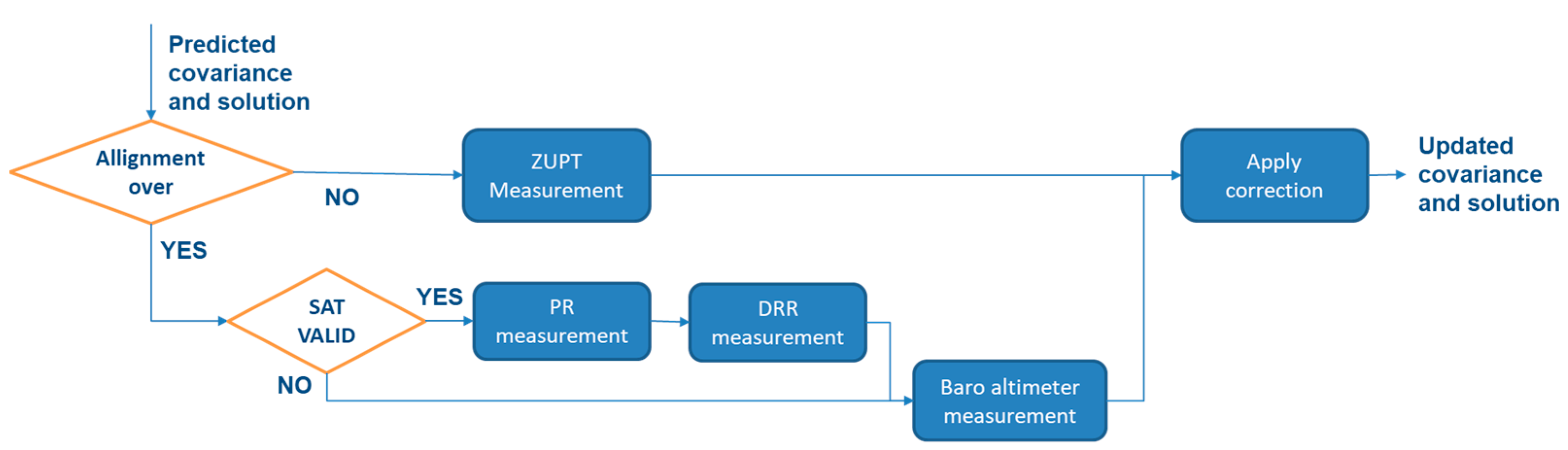
The Kalman filter update module is implemented in a single function and it adopts a cascade measurement approach, which involves combining multiple measurements from different sensors to improve the accuracy and reliability of the navigation solution (see Figure 3). These measurements include ZUPT measurements, pseudo-range measurements, delta range rate (DRR) measurements and barometric altimeter measurements.

If the system is still aligning, the KF update module only performs a ZUPT measurement through the following relations:

$${\overline{\mathit{z}}}_{\mathit{Z}\mathit{U}\mathit{P}\mathit{T}}={\overline{\mathit{V}}}_{\mathit{i}\mathit{n}\mathit{s}}-\left[0 0 0\right]-{\stackrel{̿}{\mathit{H}}}_{\mathit{Z}\mathit{U}\mathit{P}\mathit{T}}\mathit{d}\overline{\mathit{x}}$$

(50)

$${\stackrel{̿}{\mathit{H}}}_{\mathit{Z}\mathit{U}\mathit{P}\mathit{T}}=\left[\begin{array}{ccc}{\overline{0}}_{3\mathit{x}3}& {\overline{\mathit{I}}}_{3\mathit{x}3}& {\overline{0}}_{3\mathit{x}13}\end{array}\right]$$

(51)

where ${\overline{\mathit{z}}}_{\mathit{Z}\mathit{U}\mathit{P}\mathit{T}}$ is the innovation vector; ${\stackrel{̿}{\mathit{H}}}_{\mathit{Z}\mathit{U}\mathit{P}\mathit{T}}$ is the measurement matrix and $\mathit{d}\overline{\mathit{x}}$ is the updated state.

If the system is not in alignment mode and satellites are visible and valid, the first measurement to be computed is the pseudo range measurement. Innovation, measurement matrix and measurement noise are defined as follows:

$${{\mathit{z}}_{\mathit{P}\mathit{R}}={\overline{\mathit{p}\mathit{r}}}_{\mathit{G}\mathit{N}\mathit{S}\mathit{S}}-\widetilde{\overline{\mathit{p}\mathit{r}}}}_{\mathit{I}\mathit{N}\mathit{S}}-{\stackrel{̿}{\mathit{H}}}_{\mathit{P}\mathit{R}}\mathit{d}\overline{\mathit{x}}$$

(52)

where ${\widetilde{\overline{\mathit{p}\mathit{r}}}}_{\mathit{I}\mathit{N}\mathit{S}}$ is the pseudo-range predicted at INS computed position, and the measurement matrix depends on the line-of-sights vector of each visible satellite, the complete mathematical formulation is available in [25]. Then, the predicted state and covariance is updated:

$${\stackrel{̿}{\mathit{K}}}_{\mathit{P}\mathit{R}}=\left({\stackrel{̿}{\mathit{P}}}^{-}{\stackrel{̿}{\mathit{H}}}_{\mathit{P}\mathit{R}}^{\mathit{T}}\right){\left({\stackrel{̿}{\mathit{H}}}_{\mathit{P}\mathit{R}}{\stackrel{̿}{\mathit{P}}}^{-}{\stackrel{̿}{\mathit{H}}}_{\mathit{P}\mathit{R}}^{\mathit{T}}+{\stackrel{̿}{\mathit{R}}}_{\mathit{P}\mathit{R}}\right)}^{-1}$$

(53)

$$\mathit{d}\overline{\mathit{x}}=\mathit{d}\overline{\mathit{x}}+\stackrel{̿}{\mathit{K}}{\overline{\mathit{z}}}_{\mathit{P}\mathit{R}}$$

(54)

$${\stackrel{̿}{\mathit{P}}}^{+}=(\stackrel{̿}{\mathbf{I}}-{\stackrel{̿}{\mathbf{K}}}_{\mathit{P}\mathit{R}}{\stackrel{̿}{\mathbf{H}}}_{\mathit{P}\mathit{R}}){\stackrel{̿}{\mathit{P}}}^{-}$$

(55)

where ${\stackrel{̿}{\mathit{R}}}_{\mathit{P}\mathit{R}}$ is computed from the user equivalent range error (UERE) of each satellite in view.

The state covariance and correction are carried forward to the next measurement. The second measurement to be computed is the delta range rate measurement. Innovation, measurement matrix and measurement noise are defined, as follows:

$${{\overline{\mathit{z}}}_{\mathit{D}\mathit{R}\mathit{R}}={\overline{\mathit{d}\mathit{r}\mathit{r}}}_{\mathit{G}\mathit{N}\mathit{S}\mathit{S}}-\widetilde{\overline{\mathit{d}\mathit{r}\mathit{r}}}}_{\mathit{I}\mathit{N}\mathit{S}}-{\stackrel{̿}{\mathit{H}}}_{\mathit{D}\mathit{R}\mathit{R}}\mathit{d}\overline{\mathit{x}}$$

(56)

The same considerations performed for the pseudo-range measurement are valid here, the mathematical formulation is available in [25].

$${\stackrel{̿}{\mathit{K}}}_{\mathit{D}\mathit{R}\mathit{R}}=\left({\stackrel{̿}{\mathit{P}}}^{-}{\stackrel{̿}{\mathit{H}}}_{\mathit{D}\mathit{R}\mathit{R}}^{\mathit{T}}\right){({\stackrel{̿}{\mathit{H}}}_{\mathit{D}\mathit{R}\mathit{R}}{\stackrel{̿}{\mathit{P}}}^{-}{\stackrel{̿}{\mathit{H}}}_{\mathit{D}\mathit{R}\mathit{R}}^{\mathit{T}}+{\stackrel{̿}{\mathit{R}}}_{\mathit{D}\mathit{R}\mathit{R}})}^{-1}$$

(57)

$$\mathit{d}\overline{\mathit{x}}=\mathit{d}\overline{\mathit{x}}+\stackrel{̿}{\mathit{K}}{\overline{\mathit{z}}}_{\mathit{D}\mathit{R}\mathit{R}}$$

(58)

$${\stackrel{̿}{\mathit{P}}}^{+}=(\stackrel{̿}{\mathbf{I}}-{\stackrel{̿}{\mathbf{K}}}_{\mathit{D}\mathit{R}\mathit{R}}{\stackrel{̿}{\mathbf{H}}}_{\mathit{D}\mathit{R}\mathit{R}}){\stackrel{̿}{\mathit{P}}}^{-}$$

(59)

where ${\stackrel{̿}{\mathit{R}}}_{DRR}$ is supposed to be diagonal and constant.

As in the previous step, the state covariance and correction are carried forward to the next measurement. The final measurement to be calculated in the KF measure update algorithm is the barometric altimeter measurement, for which the innovation is defined as follows:

$${{\overline{\mathit{z}}}_{\mathit{B}\mathit{A}\mathit{R}\mathit{O}}={\overline{\mathit{h}}}_{\mathit{I}\mathit{N}\mathit{S}}-\overline{\mathit{h}}}_{\mathit{b}\mathit{a}\mathit{r}\mathit{o}}-{\stackrel{̿}{\mathit{H}}}_{\mathit{B}\mathit{A}\mathit{R}\mathit{O}}\mathit{d}\overline{\mathit{x}}$$

(60)

The apply correction step is utilized in the algorithm to incorporate the correction to the solution and provide feedback to the next iteration. The error state solution, relative to the last computed measurement step, is used to calculate the navigation solution. Corrections are summed to the predicted solution according to their physical meaning starting from the last state estimation $\mathit{d}\overline{\mathit{x}}={\left[\overline{\mathit{\phi }},\mathit{\delta }{\overline{\mathit{v}}}^n,\mathit{\delta }\overline{\mathit{p}},\mathit{\delta }{{\overline{\mathit{\epsilon }}}^b,\mathit{\delta }{\overline{\mathit{𝛻}}}^{\mathit{b}},\mathit{\delta }\overline{\mathit{x}}}_{\mathit{C}\mathit{l}\mathit{o}\mathit{c}\mathit{k}}\right]}^{\mathit{T}}$. The error states are then transformed into the total predicted state.

2.4. Protection Level and Figure of Merit Computation

This module performs PL and FOM computation, taking advantage of EKF covariance estimation and using the ERAIM module outputs. Indeed, it basically performs PL coasting between GNSS measurements while being suitably initialized, depending on the current operating mode and validity information coming from FDE processing of the GNSS measurement. This simple approach, derived from [34], allows PL estimation to be obtained transparently and efficiently with hybrid IMU/GNSS units even during GNSS partial or complete outages, at the only price to have a preliminary characterization of the maximum acceleration errors that can be experienced by a given IMU during a pure coasting solution. Obviously, the PL drift that is obtained depends upon the IMU quality class, but, for good fibre optic gyro units, it can also still be acceptable in safety critical operations for some minutes, which should allow the vehicle to move to a safe and more comfortable condition.

The basic steps of the PL and FOM algorithm are as follows:

• PL Initialization that selects the PL value for initialization of the PL coasting algorithm, based on the current operating mode, the status of GNSS receiver and on the current values of the KF covariance;
• PL Coasting that implements an explicit propagation of the PLs starting from suitably initial values;
• FOM Computation that computes the free fault figure of merit, with given covariance matrix of KF.

2.4.1. PL Initialization

Initial PLs shall come from the worst values between the PLs computed by ERAIM algorithm (that are inputs), if these are well defined (i.e., FD = 0 or 1 and FIX = 1), and the inflated KF covariance with the addition of the maximum non-detectable bias values.

The initial PL with EKF covariance shall be computed as follows:

$${HPL}_{KF}={H_{slope}+K}_{PL}\ast \sqrt{P_{11}^2+P_{22}^2}$$

(61)

$${VPL}_{KF}={V_{slope}+K}_{PL}\ast \sqrt{P_{33}}$$

(62)

Then, defining HPL and VPL the worst value between ERAIM PL and the above ones, the covariance reset value in north-east-down reference frame is computed as follow:

$$P_{x,0}={\displaystyle \frac{1}{K_{PL}^2}}\left(\begin{array}{ccc}{\displaystyle \frac{{HPL}^2}{2}}& 0& 0\\ 0& {\displaystyle \frac{{HPL}^2}{2}}& 0\\ 0& 0& {VPL}^2\end{array}\right)$$

(63)

$$K_{PL}={erf}^{-1}\left(1-2\ast IR\right)$$

(64)

where $IR$ is the integrity risk that is identified by the probability of missed detection as defined in the table below and erf⁻¹ is the inverse of the normal cumulative probability function.

2.4.2. PL Coasting

Starting from the covariance initial value, as determined by the above procedure, this part of the algorithm performs coasting of the covariance position and white noises, using an explicit integration formulation, as described in [34]:

$$P_{x,k}={{P_{x,0}+Q}_w∆t}^4\left({\displaystyle \frac{1}{6}}k\left(k+1\right)\left(2k+1\right)\right)$$

(65)

where $∆t$ is the sample time; $k$ (that is ≥0 and it is 0 when a covariance reset is performed) is the discrete number of samples since the integration start and $Q_w$ is a diagonal noise covariance tunable parameter (with the same noise power for every axis) that overbounds the rotation-corrected acceleration measurements with a Gaussian distribution taking into account that the simple noise integration model is based on non-rotating flat earth, perfect gravity compensation and known perfect attitude. This parameter is a characteristic of the IMU device that is used for integration with the GNSS receiver. Actually, higher quality IMUs will keep the covariance drift within acceptable values for several minutes.

When the above coasted covariance is below the KF covariance, then this last one shall be used.

The final protection levels are computed by inflating the corresponding elements of the above coasted covariance, as follows:

$${HPL}_{FF}=K_{PL}\ast \sqrt{S_{11}^2+S_{22}^2}$$

(66)

$${VPL}_{FF}=K_{PL}\ast \sqrt{S_{33}}$$

(67)

where $S_{ii}^2$, with i = 1…3 are the diagonal elements of the coasted covariance matrix in the order north, east, down for position and velocity, computed as above. $K_{PL}$ is previously defined and depends upon the IR previously defined.

2.4.3. FOM Computation

This algorithm finally computes the free fault 95% accuracy of position and velocity based on the covariance matrix of the Kalman filter, as follows:

$$HFOM=1.96\sqrt{S_{11}^2+S_{22}^2}$$

(68)

$$VFOM=1.96\sqrt{S_{33}}$$

(69)

$$VHFOM=1.96\sqrt{S_{44}^2+S_{55}^2}$$

(70)

$$VVFOM=1.96\sqrt{S_{66}}$$

(71)

where $S_{ii}^2$, with i = 1…6 are the diagonal elements of the Kalman filter covariance matrix in the order north, east, down for position and velocity.

3. Validation Test Rig and In-Flight Results

After fast-time and real-time HW in-the-loop verification of the HNU module, in-flight demonstrations have been performed exploiting an Italian Aerospace Research Centre (CIRA) flight experimental vehicle capable of executing autonomous flights. Such a vehicle is based on a modified TECNAM P92-Echo S (named FLARE) with a related ground control station and a dedicated datalink, located close to the Capua airport in CIRA premises. The HNU software was deployed on a PC-104 hardware and embarked on the RPAS as payload under test (i.e., the RPAS had its own guide, navigation and control system managing the flight while the HNU runs in parallel) in order to safely test its functionalities.

Figure 4 shows the setup for the in-flight testing. It is composed of the following:

• A GNSS receiver, model JAVAD-DELTA3, and related antenna capable of receiving GPS, Galileo and BeiDou signals;
• An IMU, model Civitanavi KRIO, based on fibre-optic gyros and quartz accelerometers;
• An air data system;
• A PC-104 platform for the RT execution of the item under test (i.e., HNU module), not involved in the control of the automatic flight (AURORA payload module in Figure 4).

Furthermore, a real-time kinematic (RTK) GPS receiver is also installed onboard and used as reference centimetre level position sensor to estimate the actual performance of the HNU in terms of position and velocity errors.

Figure 5 highlights the specific installation location of each equipment of Figure 4 on the experimental flight vehicle.

The considered use case is that of an RPAS performing a photogrammetry mission over the Rome urban area through a complete autonomous flight. The real flights have been actually performed in the Capua area while the Rome operational area has only been used to inject into the actual GNSS observables the threats related to the urban environment of Rome. That has been possible taking advantage of a GNSS threat simulator (GTS) module (see Figure 4) developed to elaborate and modify the DFMC GNSS observables in order to introduce the effects of satellite visibility (i.e., the actual visibility condition of the receiver’s antenna with respect to terrain and ground obstacles), multipath, radio frequency interference and cyber threats (i.e., jamming, spoofing) typical of an UAM scenario.

In fact, the “actual operational area” has been located around the Capua airport as required by the experimental permit to fly prescriptions while the “virtual operational area” has been located over the Rome city centre (see Figure 6) simply shifting the position by means of a constant latitude, longitude and altitude values.

In the described operational context, a spoofing threat test was executed, in which in addition to satellite visibility and multipath threats, a cyber-attack with a spoofer device was injected into the GNSS receiver.

In this test, the GTS was configured to inject the spoofing attack on all the satellites in view, in a location that is near the planned trajectory of FLARE and with a signal that has a spoofing to signal ratio of about 45 db. The scenario that resulted from the above configuration is related to a hacker who performs the spoofing attack from the roof of a building located quite close to the FLARE trajectory and activates it as soon as the vehicle is around the spoofer location. The spoofer is a meaconer that simply re-transmits to the HNU the satellite signals gathered by a GNSS receiver that is fixed in the same position of the spoofer.

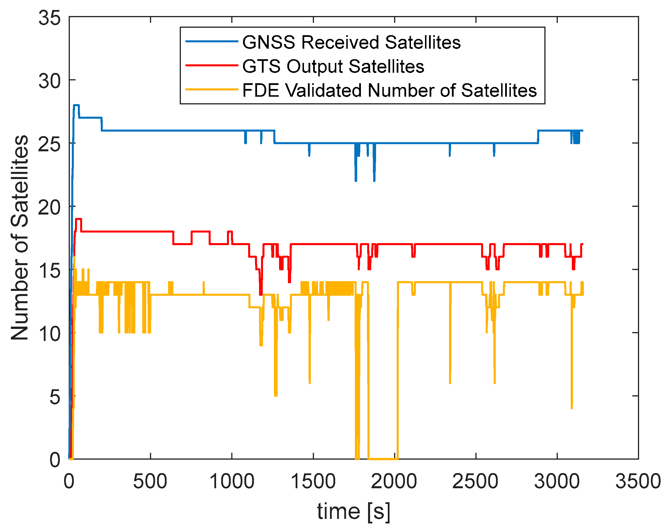
Figure 7 shows the comparison between the following:

• The GNSS-received satellites, that are the real satellites acquired by the GNSS device in the actual operational area where the aircraft is flying at about 3000 ft of altitude;
• The satellites provided by the GTS, that are the ones acquired by the GNSS device but filtered due to visibility (i.e., the RPAS is flying at about 350 ft) in the urban scenario (i.e., the virtual operational area). Figure 8 reports the mission flight plan, in terms of latitude, longitude, and terrain elevation emulated on Rome area;
• The validated satellites from the FDE algorithm, given in input the GTS measurements.

From the previous figure, the effect is clear of the reduced satellite visibility due to the surrounding terrain and obstacles of the urban scenario with respect to the actual operational area. Moreover, in the time interval between 1100 s and 1700 s, continuous changes in the FDE-validated satellites can be noted, due to the removal of those affected by the multipath effect. In fact, during that time interval, the RPAS is flying the FGH segments (see Figure 8) that are next to a mountain.

In the time interval that goes from 1700 s to about 2000 s, the effect of the cyber-attack is clear. As the GTS injects the threat, the FDE detects it and excludes all the satellites so that the HNU can continue to provide a valid solution even in these conditions taking advantage of the IMU and ADS measurements.

Finally, it is worth noting that in the first 500 s, the FDE-validated number of satellites must not be considered because the HNU is in the alignment phase, with the RPAS steady on the ground, and so the EKF and the FDE are still not fully initialized.

Figure 9 reports the trajectory performed by the vehicle from the take-off to landing in the actual operational area. It is worth noting that during the execution of the automatic flight plan, near the waypoint F (see Figure 8 and Figure 9), the flight control computer experienced a failure which required a manual recovery from the pilot. The failure autonomously detected by the flight control computer (FCC) regarded a C2 link loss. After the pilot recovery manoeuvre, the failure disappeared and the flight continued in autonomous mode as expected.

Looking to the HNU FDE status in Figure 10, it can be noted how it excludes some satellites throughout the flight due to the effects of multipath, but a larger region between 1700s and 2000s confirms the spoofing detection as induced by the GTS. Moreover, sporadic events that make all the satellites be excluded can be noted along the flight. They are associated with conditions in which the number of GPS-validated satellites is below five, determining the impossibility for the FDE to validate the GPS solution and then the satellites of the other constellations as explained in the ERAIM algorithm description section (see Section 2.2.2).

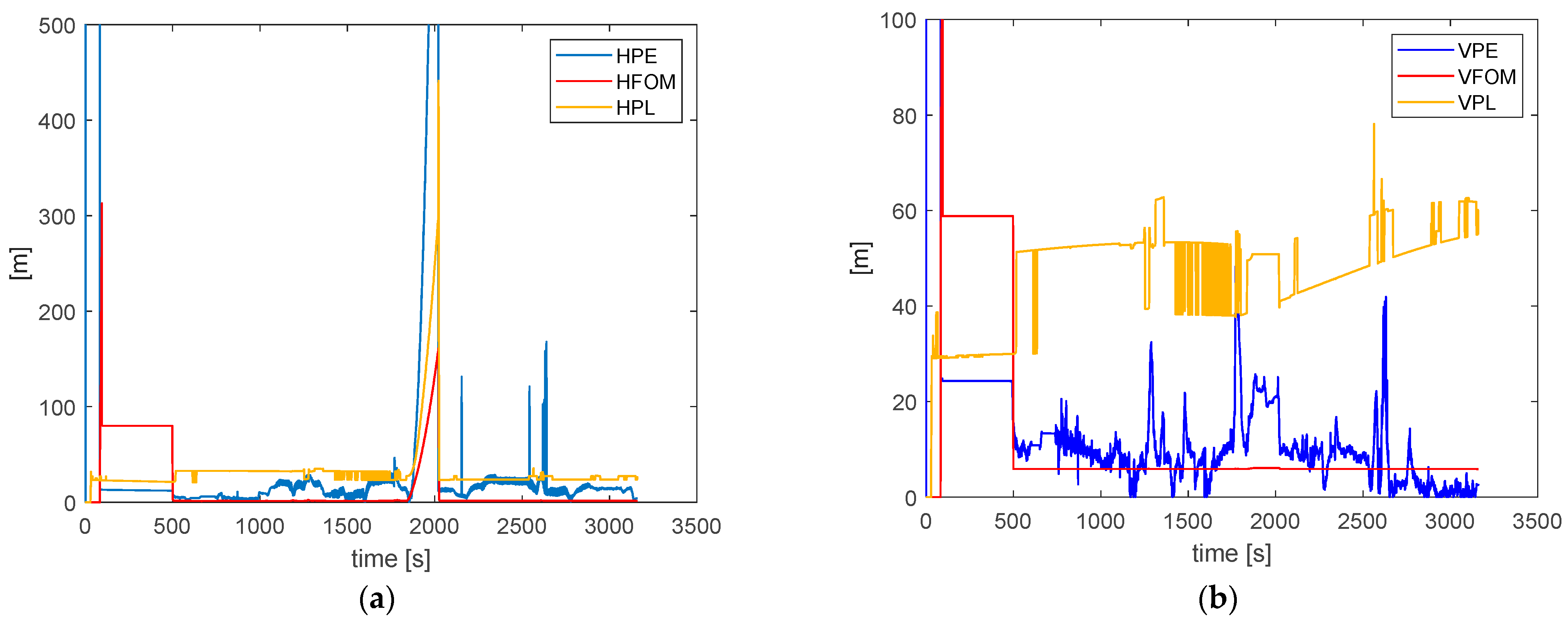
The performance of HNU in terms of position and velocity errors and related FOMs and PLs are reported in the following figures. It is evident that during this flight, the AURORA payload performed well on the horizontal but even better on the vertical due to the barometric altitude aiding.

Figure 11 shows the comparison among the position error of the HNU with respect to the RTK (used as reference for position and velocity), the figure of merit and the protection level on both the horizontal and the vertical plane. On the horizontal (see Figure 11a), during the nominal flight (i.e., without considering the time interval of application of the cyber threat), the HNU position error has a mean of 13 m with a standard deviation of about 8.5 m. It is always bounded by the computed PL except during the spoofing attack. In that case, it is evident that the horizontal position error overcomes the HPL indicating the necessity to better tune the KF. However, as soon as the cyber-attack ends, the HNU recovers the HPL. On the vertical plane, the mean of the error is about 9.2 m with a standard deviation of 6.5 m, also considering the spoofing attack time interval. In fact, in this case, the aid of the barometric measurements avoids the error to increase in time while the HNU makes a good estimation of the VPL for all the flight.

For what concerns the FOM, on the horizontal it has a mean of 2 m (not considering the spoofing interval), while on the vertical, it has a mean of 5.9 m considering all the flight (after the take-off phase).

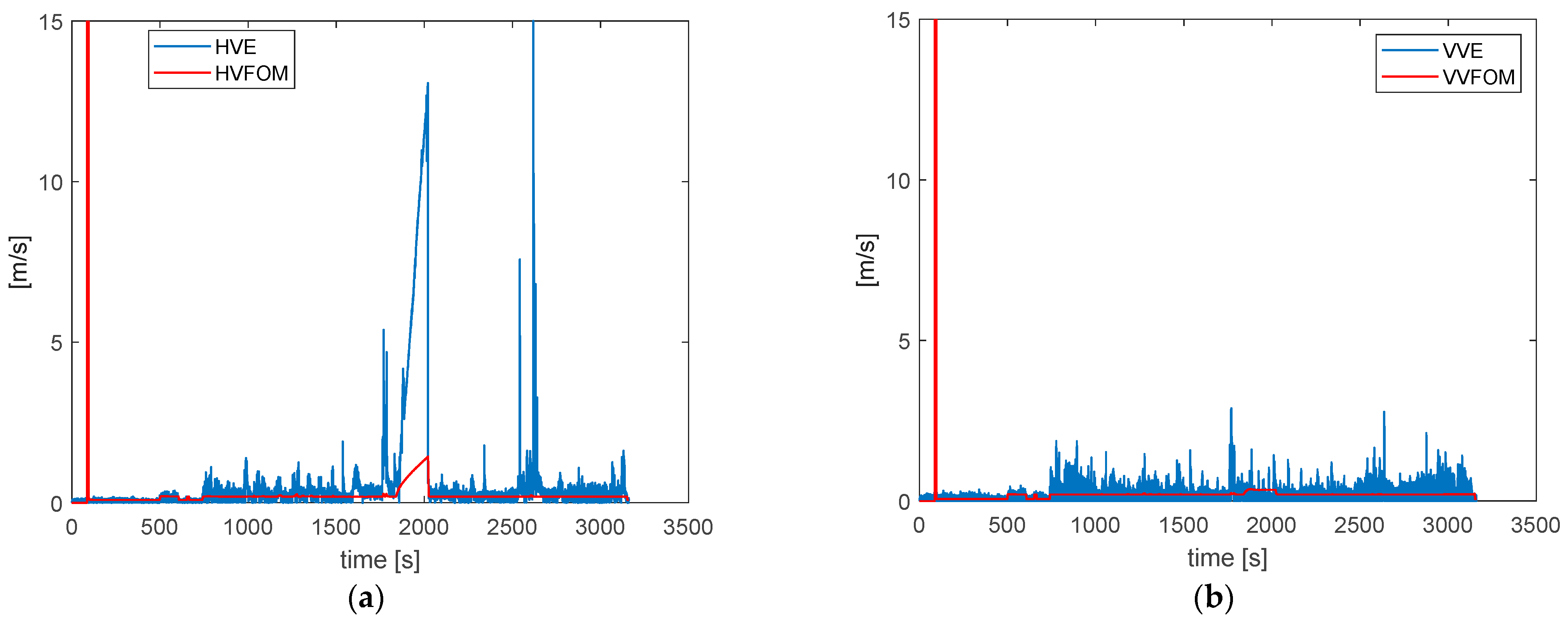
In Figure 12, the HNU performances related to the velocity are also reported. On the horizontal plane, the velocity error has a mean of about 0.6 m/s and 0.31 m/s and a standard deviation of 1.7 m/s and 0.4 m/s considering or not the spoofing time interval. On the vertical plane, the velocity error has a mean of 0.19 m/s with a standard deviation of 0.21 m/s considering all the flight phase apart from the take-off.

It is worth noting that errors are evaluated with respect of the solution of an RTK differential GPS receiver onboard and acquired from the FCC. Indeed, such RTK GPS receiver is used during the FLARE actual flights as a reference for the aircraft position and velocity solution.

In conclusion, a general underestimation of the FOMs with respect of the actual position and velocity errors has been highlighted both on the horizontal and the vertical plane. HPL behaviour is consistent on the whole trajectory, but during the coasting phase (i.e., during the cyber-attack) it underestimates the actual horizontal position error. The VPL, on the other side, is correctly estimated for the whole mission after the take-off. All these considerations imply the need to make a fine tuning of the EKF in order to have a better estimation of the navigation solution and related integrity/accuracy during cyber-attacks.

The performed tests demonstrate that the HNU is capable of providing a good estimation of the navigation solution in nominal conditions and to detect electromagnetic threats continuing to provide a valid navigation solution to the RPAS without compromising the execution of the automatic mission. This last aspect represents the main advantage of the present technique with respect of the classical approach based only on the GNSS device where also a temporary outage of the GNSS can determine the discontinuity of the PVT solution even in nominal scenarios. This is particularly evident in urban and suburban environments, where the benefits of GNSS are compromised by significant multipath effects, poor satellite visibility and electromagnetic interference. In this respect, a quantitative evaluation of the navigation solution degradation in the different GNSS satellite visibility and multi-path conditions is outside the scope of this paper. However, from a qualitative stand-point, the proposed tight coupling Kalman filter strategy can optimally use all the available satellites (even if they are below the minimum number required by a GNSS receiver), while the above results demonstrate that the satellites affected by heavy multi-path or spoofing attacks are typically removed by the proposed FDE module.

4. Conclusions

In this paper, the algorithms of a hybrid navigation unit for UAM applications were detailed. Such system implements a tightly coupled sensor fusion between a DFMC GNSS receiver (in standalone configuration), an IMU (with closed-loop fibre optic gyroscope technology and quartz accelerometer) and barometric altitude from an ADC.

The peculiarity of the system is the integration of the navigation algorithm together with autonomous fault detection and exclusion of GPS/Galileo/BeiDou satellites and estimation of navigation solution integrity/accuracy algorithms.

The implemented FDE module provides an enhanced GNSS satellite failure detection and exclusion with respect to conventional RAIM when using civil GPS, taking advantage of multi-constellation measurements. It gives in output the set of validated satellite measurements that are used by the EKF update step algorithm together with the information necessary to compute the fused protection levels and figures of merit.

The effectiveness of the proposed algorithm has been validated by means of in-flight testing using an RTK GPS receiver with centimetric precision as reference for position and velocity measurements. The HNU module has been deployed on a real-time hardware machine and embarked as payload on a RPAS capable to execute autonomous mission. For safety reasons, the real flights have been performed in the Capua area using the GTS module on board to inject in the actual GNSS observables the threats related to the urban environment of Rome (e.g., multipath, satellite poor visibility, spoofing and jamming) constituting the virtual operational area.

The results obtained have highlighted the improvement in the PNT solution of the developed HNU with respect to a GNSS pure system whose performance are lowered in urban environment. In fact, the integration with the FDE algorithm applied to multi-constellation measurements was demonstrated to be effective in the rejection of satellite failures and/or cyber-attacks continuing to guarantee the integrity of the PNT solution.

Anyway, a general underestimation of the FOMs with respect to actual position and velocity errors and the fact that, during the cyber-attack, the HPL does not bound the position error indicate the necessity to better tune the EKF.

Future works will aim at fine-tuning the implemented EKF. This will be achieved through fast-time and real-time simulations taking advantage of the data recorded during this flight test campaign, in order to achieve better estimates of the navigation solution and its related integrity/accuracy during cyber-attacks. Then, further in-flight tests will be scheduled in order to evaluate the updated HNU module functionalities.