Nonlinear Extended State Observer and Prescribed Performance Fault-Tolerant Control of Quadrotor Unmanned Aerial Vehicles Against Compound Faults

Abstract

Addressing trajectory and attitude control challenges in quadrotor UAVs amid compound faults and unknown external disturbances, this paper introduces a fault-tolerant control method predicated on nonlinear extended state observers. Initially, the UAV’s dynamic model is optimized and decoupled, forming a rapid non-singular terminal sliding mode surface that circumvents the singular phenomena typical in conventional terminal sliding mode controls. A nonlinear extended state observer is then deployed to estimate the unknown states triggered by compound faults and disturbances within the control system. Theoretical analysis shows that beyond accurately estimating faults and disturbances, the proposed controllers adaptively adjust the system’s dynamic and steady-state performances, ensuring rapid stabilization of all error responses. Numerical simulations indicate significant enhancements in control precision and robustness against compound faults and disturbances, with response times and energy consumption remaining within acceptable limits for practical applications.

1. Introduction

In recent years, quadrotor drones have attracted increasing attention from both the industrial and academic communities. Compared to traditional aircraft, quadrotors offer several advantages, such as the ability to perform vertical take-offs and landings, maintain stationary flight, fly at low speeds and altitudes, and operate indoors. They can also quickly change their flight attitudes in confined spaces [1]. As a result, quadrotors have been widely applied in numerous industries, including agriculture, atmospheric monitoring, forest fire prevention, power line and pipeline inspections, search and rescue, reconnaissance, and surveillance [2]. However, quadrotors primarily rely on the rotational speed of four propellers to control six degrees of freedom (DOF): three for position (x, y, z) and three for orientation (roll, pitch, yaw). They are a multi-input, multi-output underactuated system, highly sensitive to external disturbances, system uncertainties, and failures in actuators and sensors. This sensitivity poses significant challenges in the design of their controllers.

With the proliferation of quadrotor drones, numerous effective control theories have been developed for their management, such as sliding mode control [3,4], fuzzy control [5,6], predictive control [7,8], adaptive control [9,10], and H∞ control [11,12]. Adaptive control can adjust control parameters in real-time to cope with unknown or changing system parameters, although it may present issues with stability and computational burden. Sliding mode control is renowned for its robustness against system uncertainties, but it may induce high-frequency oscillations (chattering). Predictive control is capable of optimizing future control actions, though it demands significant computational resources. Neural networks offer a method to handle complex nonlinear systems, but they require extensive data and are difficult to analyze. Moreover, these methods do not typically assume a fault in the quadrotor systems when designing controllers. Due to their complex dynamic models, quadrotors are particularly susceptible to sensor and actuator failures, which can lead to instability in their control systems. This not only risks drone crashes, failing to complete missions, but also can cause property damage and, more severely, threaten human safety. For instance, instability in motor voltage [13,14] and malfunction of the current sensor [15] can significantly exacerbate these risks. To address these issues and enhance the reliability and safety of quadrotors during operations, fault-tolerant control (FTC) methods have been developed. The concept of FTC, which traces back to the integrity control proposed by Professor Niederlinsk in 1971 [16], has since garnered widespread attention from scholars. Existing FTC approaches can be categorized into passive fault-tolerant control (PFTC) and active fault-tolerant control (AFTC) [17]. PFTC is a strategy closely related to robust control that does not rely on fault information to manage the system, with controllers designed for robustness against predefined faults and often integrates redundancy to enhance resilience [18]. Consequently, numerous control strategies have emerged, such as those based on adaptive control [19], sliding mode control [20], predictive control [21] and neural networks [22]. Researchers have proposed adaptive sliding mode control with finite-time convergence properties to solve the hovering problem of quadrotors with unknown disturbances and actuator saturation failures, Some researchers have proposed adaptive sliding mode control with finite-time convergence characteristics to solve the hovering problem of four-rotor UAVs with unknown disturbances and actuator saturation faults, but there is no design in performance adjustment [23]. Another study presented a global fast terminal sliding mode control algorithm for quadrotors with external disturbances and actuator failures to address control issues under fault and disturbance conditions, but the fault situation does not take into account the time-varying fault [24]. There has also been a proposal for using super-twisting sliding mode control combined with a control allocation system to handle actuator faults in quadrotors, ensuring significant robustness against uncertainties and disturbances even in the presence of actuator failures [25]. However, the designed sliding mode surface exists, but there will be singular phenomena when approaching the equilibrium point. Considering the dynamics model and control input boundary constraints, researchers developed a nonlinear model predictive control (MPC) controller to enable quadrotors to recover to the desired attitude under extreme initial conditions [26], but the modeling of the four-rotor UAV ignores the gyroscopic effect and air resistance in practical applications.

In this context, researchers have proposed a fault estimation scheme based on radial basis function neural networks, accurately estimating the magnitude of faults and actively compensating for them, thus significantly improving the stability and performance of drones under fault conditions [27]. Another study presented an inversion-based sliding mode disturbance rejection attitude controller to address disturbances in quadrotor UAVs [28]. Additionally, given the model’s strong coupling and susceptibility to external disturbances, another study employed nonlinear disturbance rejection control to manage the attitude loop, aiming to enhance the robustness and trajectory tracking capabilities of quadrotor drones [29]. However, these studies primarily focus on stability while also considering dynamic performance and robustness in their controller designs, without addressing the coordination between steady-state and dynamic performance. Consequently, some researchers have adopted the prescribed performance control (PPC) developed by Bechlioulis and Rovithakis [30], proposing a novel prescribed performance-based inversion control algorithm to tackle comprehensive disturbances and trajectory tracking issues [31]. Controlling both dynamic and steady-state performance [32,33,34,35], as well as estimating unknown states to ensure the robustness of fault-tolerant control for quadrotor drones, is essential. To this end, a researcher has designed a PPC controller based on the linear extended state observer (LESO) [36] tailored for input-restricted fault dynamic models. They introduced a control framework based on an adaptive extended state observer to address internal uncertainties, external disturbances, and actuator faults [37]. Notably, while the methods employed LESO for estimating unknown states, tracking speed and accuracy were limited. Thus, a researcher introduced a novel nonlinear extended state observer (NLESO) [38] to improve the observer’s performance. Therefore, integrating NLESO with PPC for designing fault-tolerant control schemes for quadrotor drones holds significant importance.

Considering these aspects, this study aims to explore finite-time fault-tolerant control of quadrotor drones with prescribed performance. The main contributions of this research can be summarized as follows:

• Innovative Improvements in the Dynamics Model: Systematic improvements have been made to the fault dynamics model of the quadrotor UAV. This scheme effectively calculates the UAV’s attitude and position, taking into account both composite body faults and environmental disturbances. Through this approach, all state variables rapidly and accurately reach the designed sliding mode surface, thus ensuring the system globally converges to a predetermined equilibrium state within a finite time.
• Design of a Non-Singular Terminal Sliding Mode Control Surface: We have designed a full-loop rapid non-singular terminal sliding mode control surface, overcoming the common singularity issues found in traditional sliding mode control. This design not only enhances the stability of the control system but also significantly accelerates its response speed, thereby optimizing system performance and achieving rapid convergence.
• Control Strategy Based on NLESO: To address potential unknown system faults encountered by the quadrotor UAV during complex task executions, we have developed a control strategy based on the NLESO. This control strategy, integrating prescribed performance control and a sliding mode controller, can rapidly and accurately estimate unknown states in the face of unknown composite faults and external disturbances. It effectively adjusts the system’s dynamic and steady-state performance as needed, ensuring the system can reliably return to its initial state.

The organization of this paper is as follows. Section 2 describes the establishment of the quadrotor drone model and the refinement of the problem statement. Section 3 designs the prescribed performance controller based on NLESO and analyzes system stability. Section 4 describes numerical simulations, and Section 5 presents the conclusions.

2. System Model and Problem Formulation

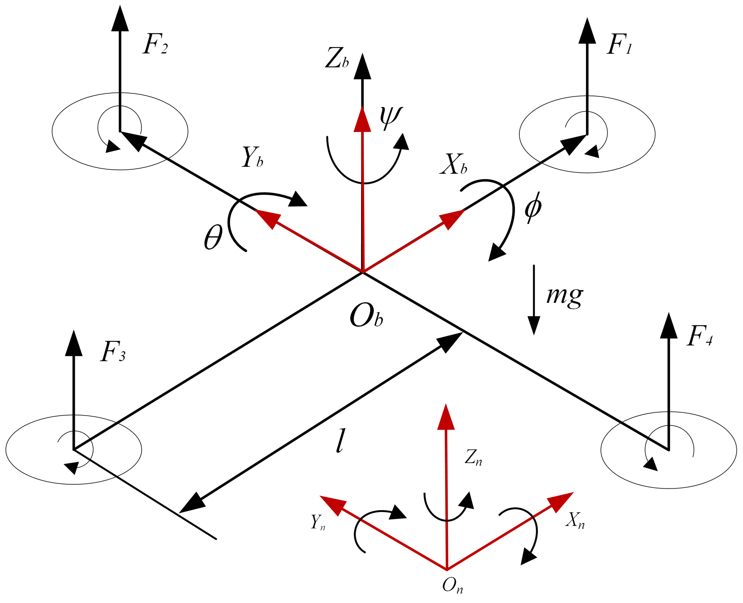
2.1. Modeling of a Quadrotor

In quadrotor unmanned aerial vehicles (UAVs), common structural configurations include the cross shape and the X shape, with the cross shape being utilized in this study. A quadrotor UAV achieves flight through the lift generated by its four propellers. The principle of flight involves altering the rotational speeds of the rotors to control the UAV’s position and attitude. To mathematically describe the position, velocity, and attitude of the quadrotor, it is essential to establish a mathematical model for the UAV. This model necessitates the creation of two coordinate systems: the earth-fixed inertial reference frame and the body-fixed reference frame. As illustrated in Figure 1, these coordinate systems are crucial for precisely describing the structure and motion principles of the quadrotor UAV and for establishing the inertial coordinate system $\left(O_n,X_n,Y_n,Z_n\right)$ and the body-fixed reference frame $\left(O_b,X_b,Y_b,Z_b\right)$ to represent the UAV’s attitude movements. Where $\mathit{l}$ represents the arm length of the UAV; $\mathit{g}$ is the acceleration of gravity; $\left(F_1,F_2,F_3,F_4\right)$ represents the lift generated by the four rotors of the UAV; and $(\varphi ,\theta ,\psi )$ is defined as the angular vector in the inertial coordinate system, representing the roll angle, pitch angle, and yaw angle, respectively. The constraints on the attitude angles are as follows: $\varphi \in (-\pi /2<\varphi <\pi /2)$, $\theta \in (-\pi /2<\varphi <\pi /2)$, $\psi \in (-\pi <\varphi <\pi )$. Then, the rotation matrix from the body coordinate system to the inertial coordinate system is as follows [39]:

$$\begin{array}{c}\hfill R_b^n=\left[\begin{array}{ccc}{C}_{\theta }{C}_{\psi }& C_{\psi }{S}_{\theta }{S}_{\varphi }-S_{\psi }{C}_{\varphi }& C_{\psi }{S}_{\theta }{C}_{\varphi }+S_{\psi }{S}_{\varphi }\\ C_{\theta }{S}_{\psi }& S_{\psi }{S}_{\theta }{S}_{\varphi }+C_{\psi }{C}_{\varphi }& S_{\psi }{S}_{\theta }{C}_{\varphi }-C_{\psi }{S}_{\varphi }\\ -S_{\theta }& S_{\theta }{C}_{\varphi }& C_{\varphi }{C}_{\theta }\end{array}\right]\end{array}$$

where ${\mathrm{S}}_{\left(·\right)}$ and ${\mathrm{C}}_{\left(·\right)}$ denote $\sin \left(·\right)$ and $\cos \left(·\right)$. For the sake of modeling convenience and without loss of generality, the following assumptions are made:

Assumption 1.

The quadrotor UAV is considered a rigid body with a symmetrical structure. During flight, gravitational acceleration is assumed constant regardless of position changes. The inertial coordinate system corresponds to the ground, and the UAV’s center of mass coincides with the origin of the body coordinate system. The lift generated by the motors is directly proportional to the square of their rotational speed.

According to the Newton–Euler method, the state space equations representing the position and attitude of the quadrotor UAV system are expressed as follows [40]:

$$\begin{array}{c}\hfill \begin{array}{cc}& \ddot{\mathbf{X}}={\displaystyle \frac{U_1}{m}}\left[\begin{array}{c}{\mathrm{C}}_{\varphi }{S}_{\theta }{\mathrm{C}}_{\psi }+S_{\varphi }{S}_{\psi }\\ {\mathrm{S}}_{\varphi }{\mathrm{S}}_{\theta }{\mathrm{C}}_{\psi }-C_{\varphi }{\mathrm{S}}_{\psi }\\ {\mathrm{C}}_{\varphi }{\mathrm{C}}_{\psi }-g\end{array}\right]-{\mathbf{F}}_{\mathbf{X}}+{\mathbf{d}}_{\mathbf{X}}\hfill \\ & {\mathbf{F}}_{\mathbf{X}}={\displaystyle \frac{{\mathbf{K}}_{\mathbf{X}}}{m}}\dot{\mathbf{X}}\hfill \\ & \ddot{\mathbf{\Theta }}={\mathbf{WU}}_{\Theta }\left[\begin{array}{c}\dot{\theta }\dot{\psi }\left(I_y-I_z\right)-J_r\varpi \dot{\theta }\\ \dot{\varphi }\dot{\psi }\left(I_z-I_x\right)-J_r\varpi \dot{\varphi }\\ \dot{\varphi }\dot{\theta }\left(I_x-I_y\right)\end{array}\right]-{\mathbf{F}}_{\mathbf{\Theta }}+{\mathbf{d}}_{\mathbf{\Theta }}\hfill \\ & {\mathbf{F}}_{\mathbf{\Theta }}=L{\mathbf{K}}_{\mathbf{\Theta }}\mathbf{W}\dot{\mathbf{\Theta }}\hfill \\ & \mathbf{W}={\left[\begin{array}{ccc}{I}_x& 0& 0\\ 0& I_y& 0\\ 0& 0& I_z\end{array}\right]}^{-1}\hfill \end{array}\end{array}$$

(1)

where $\mathbf{X}={\left[\begin{array}{c}x,y,z\end{array}\right]}^{\mathrm{T}}$ and $\mathbf{\Theta }={\left[\begin{array}{c}\varphi ,\theta ,\psi \end{array}\right]}^{\mathrm{T}}$ are defined, respectively, as the position vector and the Euler angles vector; $\varphi$ represents the roll angle, $\theta$ the pitch angle, and $\psi$ the yaw angle. ${\mathbf{U}}_{\Theta }={\left[U_2,U_3,U_4\right]}^{\mathrm{T}}$ denotes the control inputs for the quadrotor UAV in the pitch, roll, and yaw channels. ${\mathbf{K}}_{\mathbf{X}}={\left[K_x,K_y,K_z\right]}^{\mathrm{T}}$ and ${\mathbf{K}}_{\Theta }={\left[K_{\varphi },K_{\theta },K_{\psi }\right]}^{\mathrm{T}}$ represent the air resistance coefficients in each channel. $I_i(i=x,y,z)$ denotes the moment of inertia of the body about the body coordinate axes x, y, z, $\mathit{L}$ is the arm length of the UAV, $\omega$ is the sum of the rotor speeds, and $J_r$ represents the rotational inertia of the propellers. ${\mathbf{d}}_{\mathrm{X}}={\left[d_x,d_y,d_z\right]}^{\mathrm{T}}$ and ${\mathbf{d}}_{\mathbf{\Theta }}={\left[d_{\varphi },d_{\theta },d_{\psi }\right]}^{\mathrm{T}}$ denote the position disturbances experienced in each channel. These control the quadrotor UAV’s control inputs in each channel, which are related to the motor speeds as follows:

$$\left[\begin{array}{c}{U}_1\\ U_2\\ U_3\\ U_4\end{array}\right]=\left[\begin{array}{cccc}{C}_t& C_t& C_t& C_t\\ 0& -L{C}_t& 0& L{C}_t\\ -L{C}_t& 0& L{C}_t& 0\\ -C_d& C_d& -C_d& C_d\end{array}\right]\left[\begin{array}{c}{\Omega }_1^2\\ {\Omega }_2^2\\ {\Omega }_3^2\\ {\Omega }_4^2\end{array}\right]$$

(2)

where $C_t$ represents the lift coefficient and $C_d$ the drag coefficient of the quadrotor UAV, ${\Omega }_i(i=1,2,3,4)$ are motor speed.

Based on the method mentioned in [41], and considering the motor model, propeller size, and battery specifications, the maximum and minimum values of the control inputs can be determined as follows: $0\mathrm{N}\le U_1\le 16\mathrm{N}$, $-15\mathrm{Nm}\le U_2\le -15\mathrm{Nm}$, $-15\mathrm{Nm}\le U_3\le -15\mathrm{Nm}$, and $-5\mathrm{Nm}\le U_4\le -5\mathrm{Nm}$.

2.2. Establishment of Fault Model for Quadrotor UAVs

In the force analysis depicted in Figure 1, due to the effects of faults such as rotor lock, blade damage, actuator saturation, reduced motor efficiency, and loose propeller blades, it is challenging to maintain normal operation of the actuators, causing the UAV to fail in completing its predetermined tasks. Such failures can collectively be referred to as actuator failures. Depending on the modeling approach, actuator failures can be further classified into additive and multiplicative failures. Additive failures are those where the system’s output is independent of changes in control inputs. Multiplicative failures are those where the system’s output varies with changes in inputs. To facilitate a unified description and to establish a model for the actuator failures in quadrotor UAVs, it is assumed that the UAV is simultaneously affected by both additive and multiplicative actuator failures. The fault model can be represented as follows:

$$U_i^f=U_i(1-{\tau }_i)+u_{if}$$

(3)

where $U_i^f$ is the actual actuator control output, $U_i$ is the control input of each channel actuator, ${\tau }_i$ is the actuator fault coefficient, and $u_{if}$ is an unknown additive fault. The constraint range of ${\tau }_i$ is $0\le {\tau }_i\le 1$, when ${\tau }_i=0$, $u_{if}=0$, it indicates that the $\mathit{i}$-th actuator is functioning normally. When ${\tau }_i\ne 0$ and $u_{if}=0$, it indicates that the $\mathit{i}$-th actuator is only experiencing multiplicative actuator failures. When ${\tau }_i\ne 0$ and $u_{if}\ne 0$ it indicates that the $\mathit{i}$-th actuator is experiencing both multiplicative and additive failures simultaneously. Under extreme conditions ${\tau }_i=1$; it indicates that the $\mathit{i}$-th actuator has completely failed. Substituting Equation (3) into (1), the dynamic model of the quadrotor UAV, which accounts for both external position disturbances and actuator failures, can be derived as follows:

$$\begin{array}{cc}& \ddot{\mathbf{X}}={\mathbf{AU}}_X\left(1-{\tau }_X\right)+{\mathbf{u}}_{Xf}-{\mathbf{F}}_X+{\mathbf{d}}_X\hfill \\ & \ddot{\mathbf{\Theta }}=\mathbf{W}{\mathbf{U}}_{\Theta }(1-{\tau }_{\Theta })+{\mathbf{u}}_{\Theta f}+\mathbf{W}\mathbf{B}-{\mathbf{F}}_{\Theta }+{\mathbf{d}}_{\Theta }\hfill \end{array}$$

(4)

where

$$\mathbf{A}={\displaystyle \frac{1}{m}}\left[\begin{array}{c}{\mathrm{C}}_{\varphi }{\mathrm{S}}_{\theta }{\mathrm{C}}_{\psi }+S_{\varphi }{S}_{\psi }\\ {\mathrm{S}}_{\varphi }{\mathrm{S}}_{\theta }{\mathrm{C}}_{\psi }-C_{\varphi }{\mathrm{S}}_{\psi }\\ {\mathrm{C}}_{\varphi }{\mathrm{C}}_{\psi }-g\end{array}\right]$$

$$\mathbf{B}=\left[\begin{array}{c}\dot{\theta }\dot{\psi }\left(I_y-I_z\right)-J_r\varpi \dot{\theta }\\ \dot{\varphi }\dot{\psi }\left(I_z-I_x\right)-J_r\varpi \dot{\varphi }\\ \dot{\varphi }\dot{\theta }\left(I_x-I_y\right)\end{array}\right]$$

2.3. Problem Formulation

Due to the quadrotor UAV being a six-degree-of-freedom underactuated model, virtual control inputs are introduced into the position state equations to transform it into a full-drive model.

$$\left[\begin{array}{c}{U}_{1x}\\ U_{1y}\\ U_{1z}\end{array}\right]={\displaystyle \frac{U_1}{m}}\left[\begin{array}{c}{C}_{\varphi }{S}_{\theta }{C}_{\psi }+S_{\varphi }{S}_{\psi }\\ S_{\varphi }{S}_{\theta }{C}_{\psi }-C_{\varphi }{S}_{\psi }\\ C_{\varphi }{C}_{\psi }-g\end{array}\right]$$

(5)

therefore, by calculation, the desired attitude angles ${\varphi }^d$, ${\theta }^d$ and the desired lift $U_1^d$ can be represented as follows:

$$\begin{array}{c}{\varphi }^d=arctan\left(C_{\theta }{\displaystyle \frac{U_{1x}{S}_{\psi }-U_{1y}{C}_{\psi }}{U_{1z}+g}}\right)\\ {\theta }^d=arctan\left({\displaystyle \frac{U_{1x}{C}_{\psi }+U_{1y}{S}_{\psi }}{U_{1z}+g}}\right)\\ U_1^d={\displaystyle \frac{m\left(U_{1z}+g\right)}{C_{\varphi }{C}_{\varphi }}}\end{array}$$

(6)

According to Equation (6), it is evident that the quadrotor UAV achieves trajectory tracking by altering its position state through changes in attitude angles. Consequently, the position loop tracking error for the quadrotor UAV can be defined as:

$${\mathbf{e}}_X=\mathbf{X}-{\mathbf{X}}^d=\left[\begin{array}{c}{e}_x\\ e_y\\ e_z\end{array}\right]=\left[\begin{array}{c}x-x^d\\ y-y^d\\ z-z^d\end{array}\right]$$

By substituting Equation (5) into the position state equation in Equation (4), the dynamics of the position loop tracking error can be obtained:

$$\begin{array}{cc}\hfill \left[\begin{array}{c}{\ddot{e}}_x\\ {\ddot{e}}_y\\ {\ddot{e}}_y\end{array}\right]& =\left[\begin{array}{c}{U}_{1x}\left(1-{\tau }_x\right)+u_{xf}\\ U_{1y}\left(1-{\tau }_y\right)+u_{yf}\\ U_{1z}\left(1-{\tau }_z\right)+u_{zf}\end{array}\right]-{\mathbf{F}}_X+{\mathbf{d}}_X-{\ddot{\mathbf{X}}}^d\hfill \\ & ={\mathbf{U}}_{1X}\left(1-{\mathit{\tau }}_X\right)+{\mathbf{u}}_{Xf}-{\mathbf{F}}_X+{\mathbf{d}}_X-{\ddot{\mathbf{X}}}^d\hfill \end{array}$$

(7)

among $\left(U_{1X}=U_{1x},U_{1y},U_{1z}\right)$, $\left({\tau }_X={\tau }_x,{\tau }_y,{\tau }_z\right)$, $(u_{Xf}=u_{xf},u_{yf},u_{zf})$, and $F_X$, $d_X$, ${\ddot{X}}^d$ are all defined above.

Similarly, the attitude loop tracking error for the quadrotor UAV can be defined as:

$$e_{\Theta }=\Theta -{\Theta }^d=\left[\begin{array}{c}{e}_{\varphi }\\ e_{\theta }\\ e_{\psi }\end{array}\right]=\left[\begin{array}{c}\varphi -{\varphi }^d\\ \theta -{\theta }^d\\ \psi -{\psi }^d\end{array}\right]$$

then, based on the attitude state equation in Equation (4), the dynamics of the attitude loop error can be derived.

$$\left[\begin{array}{c}{\ddot{e}}_{\varphi }\\ {\ddot{e}}_{\theta }\\ {\ddot{e}}_{\psi }\end{array}\right]={\mathbf{WU}}_{\Theta }(1-{\mathit{\tau }}_{\Theta })+{\mathbf{u}}_{\Theta f}+\mathbf{WB}-{\mathbf{F}}_{\Theta }+{\mathbf{d}}_{\Theta }-{\ddot{\mathbf{\Theta }}}^d$$

(8)

Through the aforementioned transformations, the trajectory tracking problem of the quadrotor UAV is converted into a tuning problem for the position tracking error system in Equation (7), represented by ${\ddot{e}}_x$, ${\ddot{e}}_y$, ${\ddot{e}}_z$, and the attitude tracking error system in Equation (8), represented by ${\ddot{e}}_{\varphi }$, ${\ddot{e}}_{\theta }$, ${\ddot{e}}_{\psi }$. This approach allows for focused adjustments on both position and attitude errors to enhance the overall tracking performance of the UAV.

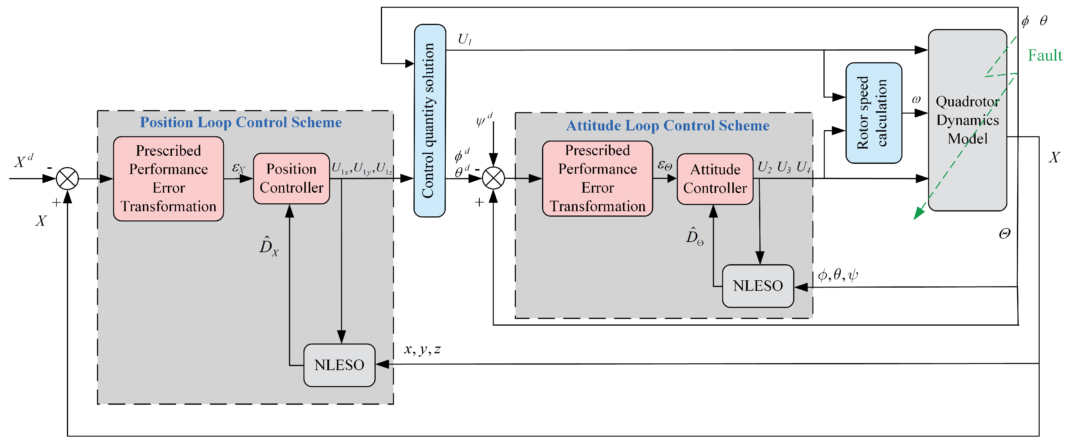
3. Prescribed Performance Controller Design

In this section, a prescribed performance fault-tolerant controller based on a nonlinear extended state observer is designed for the quadrotor UAV model, which accounts for actuator faults and unknown external disturbances. This controller aims to ensure trajectory and attitude tracking of the quadrotor UAV. The framework of the controller is illustrated in Figure 2. This design integrates the observer’s ability to estimate the system states and disturbances in real-time, enabling the controller to compensate effectively, thus maintaining robust performance even in the face of system anomalies or external interferences.

3.1. Prescribed Performance Control Concept

In the attitude tracking control of quadrotor UAVs, it is nearly impossible to make the tracking error converge to zero immediately, and overshoot can potentially reach high values, which increases the uncontrollability risk during the UAV’s flight. To address this issue, a feasible control strategy, namely prescribed performance control (PPC), is employed to impose certain constraints on the tracking error, ensuring that the system maintains satisfactory transient and steady-state performance within defined boundaries. This section summarizes preliminary knowledge about PPC. With prescribed performance, it means that the attitude errors $e_{\varphi }$, $e_{\theta }$, and $e_{\psi }$ are strictly confined within a predefined region bounded by a time-decaying performance function. The mathematical form of the specified performance function is represented by the inequality:

$$\begin{array}{c}\hfill -M_i{\rho }_i\left(t\right)<e_i\left(t\right)<{\rho }_i\left(t\right),if{e}_i\left(0\right)\ge 0\\ \hfill -{\rho }_i\left(t\right)<e_i\left(t\right)<M_i{\rho }_i\left(t\right),if{e}_i\left(0\right)\le 0\end{array}$$

(9)

where $0\le M_i\le 1$, $i\in \left\{\begin{array}{c}\varphi ,\theta ,\psi \end{array}\right\}$ is the constraint on the performance boundary. The performance function, denoted as ${\rho }_i\left(t\right)$, is smooth, bounded, and strictly monotonically decreasing. This ensures that the performance constraints adapt over time, tightening as the system approaches the desired steady state, thus providing a controlled and predictable reduction in the tracking errors. The performance function ${\rho }_i\left(t\right)$ is chosen as:

$${\rho }_i\left(t\right)=({\rho }_{i0}-{\rho }_{i\infty })e^{-l_{i}t}+{\rho }_{i\infty }$$

(10)

where $i\in \{\mathrm{X},\Theta \}$, $\left(X=x,y,z\right)$, with strict positive constants ${\rho }_{i0}$, ${\rho }_{i\infty }$ and $-l_i$, $i\in \{\mathrm{X},\Theta \}$. ${\rho }_{i0}$ determines the initial state of the performance function, ${\rho }_{i\infty }$ represents the maximum performance boundary when the system reaches steady state, and $l_i$ controls the rate of convergence of the system. These parameters are crucial for tailoring the performance function to specific requirements, ensuring that the system not only meets initial performance expectations but also converges to a steady state within acceptable boundaries and at a desirable rate.

Due to the introduction of the performance function, the control system has incorporated additional constraints, which complicates the design of the controller. Therefore, after completing the design of the predefined performance function, it is necessary to transform the constrained control problem into an unconstrained control problem through a homeomorphic mapping, achieving an isomorphic mapping of the space. The definition is

$$e_i\left(t\right)=E_i\left({\epsilon }_i\right){\rho }_i\left(t\right)$$

(11)

and the transformation function is selected as follows:

$$E_i\left({\epsilon }_i\right)={\displaystyle \frac{exp\left({\epsilon }_i\right)-exp(-{\epsilon }_i)}{exp\left({\epsilon }_i\right)+exp(-{\epsilon }_i)}}$$

(12)

The error in the unconstrained system following the homeomorphic mapping, denoted as ${\epsilon }_i$, is the transformation error. It is a smooth and completely monotonically function. The specific expression for ${\epsilon }_i$ is given as:

$${\epsilon }_i=E_i^{-1}\left({\displaystyle \frac{e_i\left(t\right)}{{\rho }_i\left(t\right)}}\right)$$

(13)

From this, the expression for the transformed error can be derived as:

$${\epsilon }_i={\displaystyle \frac{1}{2}}ln\left({\displaystyle \frac{M_i+\upsilon }{M_i-\upsilon }}\right)$$

(14)

where $v=e_i\left(t\right)/{\rho }_i\left(t\right)$. With this, the final expression for the transformed error is derived to serve as the terminal sliding mode variable, thus preparing the groundwork for deriving the control input in the subsequent discussion.

To obtain the first derivative of the transformed error (14), differentiate it with respect to time. This will provide the expression for the first derivative of the transformed error:

$${\dot{\epsilon }}_i=\chi \left({\dot{e}}_i-e_i{\displaystyle \frac{{\dot{\rho }}_i}{{\rho }_i}}\right)$$

(15)

where $\chi ={\displaystyle \frac{1}{2\rho }}\left({\displaystyle \frac{1}{\epsilon +M}}-{\displaystyle \frac{1}{\epsilon -M}}\right)$ is a bounded variable, and its constraints are defined by $0\le \chi \le {\chi }_{max}\left({\chi }_{max}>0\right)$.

To obtain the second derivative of the transformed error (14), differentiate the first derivative with respect to time. This will provide the expression for the second derivative of the transformed error:

$$\ddot{\epsilon }=\dot{\chi }\left({\dot{e}}_i-e_i{\displaystyle \frac{\dot{\rho }}{\rho }}\right)+\chi \left({\ddot{e}}_i-{\dot{e}}_i{\displaystyle \frac{\dot{\rho }}{\rho }}-e{\displaystyle \frac{\ddot{\rho }}{\rho }}+e{\rho }^2\right)$$

(16)

where

$$\begin{array}{cc}\hfill \dot{\chi }& =-{\displaystyle \frac{\dot{\rho }}{2\rho }}\left({\displaystyle \frac{1}{\epsilon +M}}-{\displaystyle \frac{1}{\epsilon -M}}\right)-{\displaystyle \frac{\dot{e}\rho -e\dot{\rho }}{2{\rho }^3}}\left({\displaystyle \frac{1}{{\left(\epsilon +M\right)}^2}}-{\displaystyle \frac{1}{{\left(\epsilon -M\right)}^2}}\right)\hfill \end{array}$$

(17)

3.2. NLESO Design

(1)

Design of NLESO for position loop

To estimate the unknown external disturbances $D_X,\left(X=x,y,z\right)$ in the position loop, a nonlinear extended state observer is designed based on the dynamics of the position loop tracking error system (7) as follows:

$$\left\{\begin{array}{ll}{\sigma }_X^1& =z_{X_1}-{\dot{\epsilon }}_X\\ fe\hfill & =fal\left(\sigma ,\alpha ,h\right)\\ {\dot{z}}_{X_1}\hfill & =U_{1X}\left(1-{\tau }_X\right)+u_{Xf}-F_X-{\ddot{X}}^d+z_{X_2}-{\beta }_{X_1}fe\\ {\dot{z}}_{X_2}\hfill & =-{\beta }_{X_2}fe\\ {\widehat{D}}_X\hfill & =z_{X_2}\end{array}\right.$$

(18)

where ${\sigma }_X^1$ and ${\sigma }_X^2$ define the observer errors. The coefficients ${\beta }_{X_1}$ and ${\beta }_{X_2}$ are observer gain coefficients, which are positive constants. ${\widehat{D}}_X$ is the estimated value of the external unknown disturbance $D_X$. The function fal is a defined nonlinear function, whose form is given as:

$$fal\left(\sigma ,\alpha ,h\right)=\left\{\begin{array}{c}{\displaystyle \frac{\sigma }{h^{\left(1-\alpha \right)}}},\left|\sigma \right|\le h\hfill \\ {\left|\sigma \right|}^{\alpha }sign\left(\sigma \right),\left|\sigma \right|>h\hfill \end{array}\right.$$

(19)

where $0<\alpha <1$, $h(h>0)$ is the filter factor.

(2)

Design of NLESO for attitude loop

To estimate the unknown external disturbances $D_{\Theta }\left(\Theta =\varphi ,\theta ,\psi \right)$ in the attitude loop, a nonlinear extended state observer is designed based on the dynamics of the attitude loop tracking error system (8) as follows:

$$\left\{\begin{array}{ll}{\sigma }_{\Theta }^1\hfill & =z_{{\Theta }_1}-{\dot{\epsilon }}_{\Theta }\\ fe\hfill & =fal\left(\sigma ,\alpha ,h\right)\\ {\dot{z}}_{{\Theta }_1}\hfill & =W{U}_{\Theta }\left(1-{\tau }_{\Theta }\right)+u_{\Theta f}+WB-F_{\Theta }-{\ddot{\Theta }}^d+z_{{\Theta }_2}-{\beta }_{{\Theta }_1}fe\\ {\dot{z}}_{{\Theta }_2}\hfill & =-{\beta }_{{\Theta }_2}fe\\ {\widehat{D}}_{\Theta }\hfill & =z_{{\Theta }_2}\end{array}\right.$$

(20)

where ${\sigma }_{\Theta }^1$ and ${\sigma }_{\Theta }^2$ define the observer errors. The coefficients ${\beta }_{{\Theta }_1}$ and ${\beta }_{{\Theta }_2}$ are observer gain coefficients, which are positive constants. ${\widehat{D}}_{\Theta }$ is the estimated value of the external unknown disturbance $D_{\Theta }$. The function fal is defined by Equation (19) as a specific nonlinear function.

Proof. 

First, to facilitate the analysis of the performance of the nonlinear extended state observer, the fal function is transformed as follows:

$$fal\left(\sigma ,\alpha ,h\right)={\displaystyle \frac{fal\left(\sigma ,\alpha ,h\right)}{\sigma }}\sigma =\lambda \left(\sigma \right)·\sigma$$

(21)

Since the proof process for the nonlinear extended state observers for both attitude and position are similar, they are unified into a single general formula for solving and proving their stability. Simplifying the nonlinear extended state observer by using Equation (21) and the error dynamics equation transforms it into a linear time-varying gain extended state observer, whose expression is as follows:

$$\left\{\begin{array}{c}{\sigma }^1=z_1-\dot{\epsilon }\hfill \\ fe=fal\left(\sigma ,\alpha ,h\right)\hfill \\ {\dot{z}}_1=T\left(u\right)+z_2-{\beta }_1\lambda \left({\sigma }^1\right)·\sigma \hfill \\ {\dot{z}}_2=-{\beta }_2\lambda \left({\sigma }^1\right)·\sigma \hfill \\ \widehat{D}=z_2\hfill \end{array}\right.$$

(22)

In this case, when it is a position loop nonlinear extended state observer, it is denoted by $T\left(u\right)=U_{1X}\left(1-{\tau }_X\right)+u_{Xf}-F_X-{\ddot{X}}^d$, and when it is an attitude loop nonlinear extended state observer, it is denoted by $T\left(u\right)=W{U}_{\Theta }\left(1-{\tau }_{\Theta }\right)+u_{\Theta f}+WB-F_{\Theta }-{\ddot{\Theta }}^d$. By performing a Laplace transform on Equation (22), the transfer function for the estimated state error can be derived as follows:

$$\begin{array}{cc}\hfill z_1& ={\displaystyle \frac{s{\beta }_1\lambda \left({\sigma }^1\right)+{\beta }_2\lambda \left({\sigma }^1\right)}{s^2+s{\beta }_1\lambda \left({\sigma }^1\right)+{\beta }_2\lambda \left({\sigma }^1\right)}}\epsilon \left(s\right)+{\displaystyle \frac{s}{s^2+s{\beta }_1\lambda \left({\sigma }^1\right)+{\beta }_2\lambda \left({\sigma }^1\right)}}T\left(s\right)\hfill \end{array}$$

(23)

$$\begin{array}{cc}\hfill z_2& ={\displaystyle \frac{-s}{s^2+s{\beta }_1\lambda \left({\sigma }^1\right)+{\beta }_2\lambda \left({\sigma }^1\right)}}\epsilon \left(s\right)-{\displaystyle \frac{{\beta }_2\lambda \left({\sigma }^1\right)}{s^2+s{\beta }_1\lambda \left({\sigma }^1\right)+{\beta }_2\lambda \left({\sigma }^1\right)}}T\left(s\right)\hfill \end{array}$$

(24)

For Equations (23) and (24), the characteristic equations can be derived as follows:

$$s^2+s{\beta }_1\lambda \left({\sigma }^1\right)+{\beta }_2\lambda \left({\sigma }^1\right)=0$$

(25)

according to the Routh–Hurwitz criterion, the necessary and sufficient condition for the stability of this system is as follows:

$$\left\{\begin{array}{c}{\beta }_1\lambda \left({\sigma }^1\right)>0\\ {\beta }_2\lambda \left({\sigma }^1\right)>0\end{array}\right.$$

(26)

Substituting the Equation (19) into (21), the form of $\lambda \left(\sigma \right)$ can be derived as follows:

$$\lambda \left(\sigma \right)={\displaystyle \frac{fal\left(\sigma ,\alpha ,h\right)}{\sigma }}=\left\{\begin{array}{c}\begin{array}{c}{\displaystyle \frac{1}{h^{\left(1-\alpha \right)}}},\left|\sigma \right|\le h\hfill \\ {\left|\sigma \right|}^{\alpha -1},\left|\sigma \right|>h\hfill \end{array}\end{array}\right.$$

(27)

Due to $0<\alpha <1$ and $h>0$ it can be inferred that $\lambda \left(\sigma \right)>0$ holds, and because of ${\beta }_1,{\beta }_2>0$, it follows that Equation (26) is always satisfied. This means that all poles of the characteristic Equation (25) are located in the left half of the s-plane, thereby confirming that the nonlinear extended state observer is stable. □

3.3. Design of Position Fault-Tolerant Controller

To ensure that the state variables in the position control system converge to zero, the position transformed error of the system is defined according to Equation (14) as follows:

$${\epsilon }_X={\left[\begin{array}{ccc}{\epsilon }_x& {\epsilon }_y& {\epsilon }_z\end{array}\right]}^T$$

(28)

Substituting Equation (5) into Equation (4), the modified position loop dynamic model can be obtained as:

$$\ddot{X}=U_{1X}\left(1-{\tau }_X\right)+u_{Xf}-F_X+D_X$$

(29)

In this paper, a full-loop fast non-singular terminal sliding mode surface is selected to construct the controller, which, based on the condition of position conversion error, can be expressed as:

$$s_X={\dot{\epsilon }}_X+b_X{\epsilon }_X+c_X{{\epsilon }_X}^{{\displaystyle \frac{n_X}{m_X}}}$$

(30)

where $b_X,c_X>0$, $m_X>n_X>0$, $0<{\displaystyle \frac{n_X}{m_X}}<1$, and n, m are both odd numbers. To derive the first-order derivative of Equation (30), we obtain

$${\dot{s}}_X={\ddot{\epsilon }}_X+b_X{\dot{\epsilon }}_X+c{\displaystyle \frac{n_X}{m_X}}{\dot{\epsilon }}_X{{\epsilon }_X}^{{\displaystyle \frac{n_X}{m_X}}-1}$$

(31)

The sliding mode reaching law is selected as:

$${\dot{s}}_{Xi}=-k_{X_1}{s}_X-k_{X_2}sgn\left(s_X\right)$$

(32)

where $i=1,2,3$ correspond to the approaching laws for the x, y, z channels, respectively.

To tackle the vibration issues in quadrotor unmanned aerial vehicle (UAV) systems, an improved continuous function with relay characteristics, denoted as function $\delta (•)$, is utilized to replace the sign function, referred to as function sgn(·). This substitution aims to shorten the delay time in switching control, thereby alleviating the vibration problems of the system. The expression for the continuous function $\delta (•)$ is as follows:

$$\delta \left(s_i\right)={\displaystyle \frac{2}{\pi }}arctan\left(s_i\right)$$

(33)

By substituting the second derivative of the transformation error, given by Equation (14), and the dynamics model, represented by Equation (29), the virtual control law is derived as follows:

$$\begin{array}{cc}\hfill & U_{1x}={\displaystyle \frac{1}{{\tau }_x}}(\ddot{x}+F_x-e_x{\rho }_x^2+e_x{\displaystyle \frac{{\ddot{\rho }}_x}{{\rho }_x}}+{\dot{e}}_x{\displaystyle \frac{{\dot{\rho }}_x}{{\rho }_x}}\hfill \\ \hfill & +{\displaystyle \frac{1}{{\chi }_x}}({\dot{s}}_{x1}-b_x{\dot{\epsilon }}_x-c_x{\displaystyle \frac{n_x}{m_x}}{\dot{\epsilon }}_x{{\epsilon }_x}^{\frac{n_x}{m_x}-1}-{\dot{\chi }}_x({\dot{e}}_x-e_x{\displaystyle \frac{{\dot{\rho }}_x}{{\rho }_x}}\left)\right)\hfill \\ \hfill & -{\widehat{D}}_x\delta (s_x)-u_{xf}\delta (s_x){\displaystyle )}\hfill \end{array}$$

(34)

$$\begin{array}{cc}\hfill & U_{1y}={\displaystyle \frac{1}{{\tau }_y}}(\ddot{y}+F_y-e_y{\rho }_y^2+e_y{\displaystyle \frac{{\ddot{\rho }}_y}{{\rho }_y}}+{\dot{e}}_y{\displaystyle \frac{{\dot{\rho }}_y}{{\rho }_y}}\hfill \\ \hfill & +{\displaystyle \frac{1}{{\chi }_y}}({\dot{s}}_{y2}-b_y{\dot{\epsilon }}_y-c_y{\displaystyle \frac{n_y}{m_y}}{\dot{\epsilon }}_y{{\epsilon }_y}^{\frac{n_y}{m_y}-1}-{\dot{\chi }}_y({\dot{e}}_y-e_y{\displaystyle \frac{{\dot{\rho }}_y}{{\rho }_y}}))\hfill \\ \hfill & -{\widehat{D}}_y\delta \left(s_y\right)-u_{yf}\delta \left(s_y\right))\hfill \end{array}$$

(35)

$$\begin{array}{cc}\hfill & U_{1z}={\displaystyle \frac{1}{{\tau }_z}}\left(\ddot{z}+F_z-e_z{\rho }_z^2+e_z{\displaystyle \frac{{\ddot{\rho }}_z}{{\rho }_z}}+{\dot{e}}_z{\displaystyle \frac{{\dot{\rho }}_z}{{\rho }_z}}\right.\hfill \\ \hfill & +{\displaystyle \frac{1}{{\chi }_z}}\left({\dot{s}}_{z3}-b_z{\dot{\epsilon }}_z-c_z{\displaystyle \frac{n_z}{m_z}}{\dot{\epsilon }}_z{{\epsilon }_z}^{\frac{n_z}{m_z}-1}-{\dot{\chi }}_z\left({\dot{e}}_z-e_z{\displaystyle \frac{{\dot{\rho }}_z}{{\rho }_z}}\right)\right)\hfill \\ \hfill & +g-{\widehat{D}}_z\delta \left(s_z\right)-u_{zf}\delta \left(s_z\right))\hfill \end{array}$$

(36)

where ${\widehat{D}}_x$, ${\widehat{D}}_y$, ${\widehat{D}}_z$ are obtained from the observer denoted as Equation (18), and they satisfy

$$\begin{array}{cc}\hfill & k_{x_2}>p_x,p_x>0,k_{y_2}>p_y,p_y>0,k_{z_2}>p_z,p_z>0\hfill \\ \hfill & {\left|d_1-{\widehat{D}}_1\right|}_{max}\le p_x,{\left|d_2-{\widehat{D}}_2\right|}_{max}\le p_y,{\left|d_3-{\widehat{D}}_3\right|}_{max}\le p_z\hfill \end{array}$$

(37)

Theorem 1

([42]). Suppose there exists a positive definite and continuous function $F\left(x_0\right)$ that satisfies inequality $\dot{F}\left(x_0\right)+bF\left(x\right)+cF{\left(x\right)}^{\frac{n}{m}}\le 0$, where b, c > 0, n and m are positive odd integers with n < m. If the system starts from an initial state $x_0$, then the state x will converge to an equilibrium point within a finite time ts and satisfy inequality

$$t_s\le {\displaystyle \frac{m}{b\left(m-n\right)}}ln\left({\displaystyle \frac{bF{\left(x_0\right)}^{\frac{m-n}{n}}+c}{c}}\right)$$

(38)

To analyze the stability of the system with the designed virtual controllers $U_{1x}$, $U_{1y}$, $U_{1z}$, the following Lyapunov function is selected:

$$V_1={\displaystyle \frac{1}{2}}\sum _{X\in \left(x,y,z\right)}{s}_X^2$$

(39)

then, the derivative is calculated as follows:

$$\begin{array}{cc}\hfill & {\dot{V}}_1=\sum _{X\in \left(x,y,z\right)}{s}_X{\dot{s}}_X\hfill \\ \hfill & =s_x(-k_{x_1}{s}_x-k_{x_2}sgn(s_x))+s_y\left(-k_{y_1}{s}_y-k_{y_2}sgn\left(s_y\right)\right)+s_z(-k_{z_1}{s}_z-k_{z_2}sgn(s_z))\hfill \\ \hfill & =-\sum _{X\in \left(x,y,z\right)}{k}_{X_1}{s}_X^2-\sum _{X\in \left(x,y,z\right)}{k}_{X_2}{s}_{X}sgn\left(s_X\right)\hfill \\ \hfill & =-\sum _{X\in \left(x,y,z\right)}{k}_{X_1}{s}_X^2+k_{X_2}\left|s_X\right|\hfill \end{array}$$

(40)

Because $k_{i1}$, $k_{i2}$,$(i=x,y,z)$ are known positive constants, it follows that ${\dot{V}}_1<0$. According to Theorem 1, it is known that the position loop sliding surface, $S_X$$(X=x,y,z)$, will converge to the equilibrium point within a finite time. The convergence time is

$$t_{s_X}\le {\displaystyle \frac{m_X}{b_X\left(m_X-n_X\right)}}ln\left({\displaystyle \frac{b_{X}F{\left(x_0\right)}^{\frac{m_X-n_X}{n_X}}+c_X}{c_X}}\right)$$

(41)

The analysis above demonstrates that the position loop control system can achieve the desired system state within a finite time. This subsystem is asymptotically stable.

3.4. Design of Attitude Fault-Tolerant Controller

To ensure that the state variables in the attitude control system converge to zero, the attitude transformed error of the system is defined according to Equation (14) as follows:

$${\epsilon }_{\Theta }={\left[\begin{array}{ccc}{\epsilon }_{\varphi }& {\epsilon }_{\theta }& {\epsilon }_{\psi }\end{array}\right]}^T$$

(42)

In this paper, the full-loop fast non-singular terminal sliding mode surface is selected to construct the controller. According to the attitude conversion error, the form can be expressed as:

$$s_{\Theta }={\dot{\epsilon }}_{\Theta }+b_{\Theta }{\epsilon }_{\Theta }+c_{\Theta }{{\epsilon }_{\Theta }}^{{\displaystyle \frac{n_{\Theta }}{m_{\Theta }}}}$$

(43)

where $b_{\Theta },c_{\Theta }>0$, $m_{\Theta }>n_{\Theta }>0$, $0<{\displaystyle \frac{n_{\Theta }}{m_{\Theta }}}<1$, and $n_{\Theta }$, $m_{\Theta }$ are odd numbers. The derivative of Equation (43) is obtained as follows:

$${\dot{s}}_{\Theta }={\ddot{\epsilon }}_{\Theta }+b_{\Theta }{\dot{\epsilon }}_{\Theta }+c_{\Theta }{\displaystyle \frac{n_{\Theta }}{m_{\Theta }}}{\dot{\epsilon }}_{\Theta }{{\epsilon }_{\Theta }}^{{\displaystyle \frac{n_{\Theta }}{m_{\Theta }}}-1}$$

(44)

Based on the fault dynamics model (4), the attitude subsystem can be simplified as:

$$\left\{\begin{array}{c}\ddot{\varphi }={\displaystyle \frac{1}{I_x}}\left(U_2(1-{\tau }_{\varphi })+u_{\varphi f}\right)+f_{\varphi }+d_4\\ \ddot{\theta }={\displaystyle \frac{1}{I_y}}\left(U_3(1-{\tau }_{\theta })+u_{\theta f}\right)+f_{\theta }+d_5\\ \ddot{\psi }={\displaystyle \frac{1}{I_z}}\left(U_4(1-{\tau }_{\psi })+u_{\psi f}\right)+f_{\psi }+d_6\end{array}\right.$$

(45)

where the $f_{\varphi }\left(x\right)$, $f_{\varphi }\left(x\right)$, $f_{\psi }\left(x\right)$ are defined as:

$$\begin{array}{cc}\hfill & f_{\varphi }=\dot{\theta }\dot{\psi }{\displaystyle \frac{I_y-I_z}{I_x}}-\dot{\theta }\varpi {\displaystyle \frac{J_r}{I_x}}-l{\displaystyle \frac{K_4}{I_x}}\dot{\theta }\hfill \end{array}$$

(46)

$$\begin{array}{cc}\hfill & f_{\theta }=\dot{\varphi }\dot{\psi }{\displaystyle \frac{I_z-I_x}{I_y}}-\dot{\varphi }\varpi {\displaystyle \frac{J_r}{I_y}}-l{\displaystyle \frac{K_5}{I_x}}\dot{\varphi }\hfill \end{array}$$

(47)

$$\begin{array}{cc}\hfill & f_{\psi }=\dot{\varphi }\dot{\theta }{\displaystyle \frac{I_x-I_y}{I_z}}-l{\displaystyle \frac{K_6}{I_z}}\dot{\psi }\hfill \end{array}$$

(48)

The sliding mode reaching law is selected as:

$${\dot{s}}_{\Theta i}=-k_{{\Theta }_1}{s}_{\Theta }-k_{{\Theta }_2}sgn\left(s_{\Theta }\right)$$

(49)

By substituting and transforming the attitude dynamics model (4) and the conversion error (16), the design of the controller can be derived as:

$$\begin{array}{cc}\hfill U_2& ={\displaystyle \frac{1}{1-{\tau }_{\varphi }}}\left(I_x\right({\ddot{\varphi }}_d-f_{\varphi }-{\widehat{D}}_4\delta \left(s_{\varphi }\right)-e_{\varphi }{\rho }_{\varphi }^2\hfill \\ \hfill & +e{\displaystyle \frac{{\ddot{\rho }}_{\varphi }}{{\rho }_{\varphi }}}+{\dot{e}}_{\varphi }{\displaystyle \frac{{\dot{\rho }}_{\varphi }}{{\rho }_{\varphi }}}+{\displaystyle \frac{1}{{\chi }_{\varphi }}}({\dot{s}}_{{\varphi }_1}-b{\dot{\epsilon }}_{\varphi }-c{\displaystyle \frac{n_{\varphi }}{m_{\varphi }}}{\dot{\epsilon }}_{\varphi }{\dot{\epsilon }}_{\varphi }^{{\displaystyle \frac{n_{\varphi }}{m_{\varphi }}}-1}\hfill \\ \hfill & -{\dot{\chi }}_{\varphi }({\dot{e}}_{\varphi }-e_{\varphi }{\displaystyle \frac{{\dot{\rho }}_{\varphi }}{{\rho }_{\varphi }}})\left)\right)-u_{\varphi f})\hfill \end{array}$$

(50)

$$\begin{array}{cc}\hfill U_3& ={\displaystyle \frac{1}{1-{\tau }_{\theta }}}\left(I_y\right({\ddot{\theta }}_d-f_{\theta }-{\widehat{D}}_5\delta \left(s_{\theta }\right)-e_{\theta }{\rho }_{\theta }^2\hfill \\ \hfill & +e_{\theta }{\displaystyle \frac{{\ddot{\rho }}_{\theta }}{{\rho }_{\theta }}}+{\dot{e}}_{\theta }{\displaystyle \frac{{\dot{\rho }}_{\theta }}{{\rho }_{\theta }}}+{\displaystyle \frac{1}{{\chi }_{\theta }}}({\dot{s}}_{{\theta }_2}-b{\dot{\epsilon }}_{\theta }-c{\displaystyle \frac{n_{\theta }}{m_{\theta }}}{\dot{\epsilon }}_{\theta }{\epsilon }^{{\displaystyle \frac{n_{\theta }}{m_{\theta }}}-1}\hfill \\ \hfill & -{\dot{\chi }}_{\theta }({\dot{e}}_{\theta }-e_{\theta }{\displaystyle \frac{{\dot{\rho }}_{\theta }}{{\rho }_{\theta }}})\left)\right)-u_{\theta f})\hfill \end{array}$$

(51)

$$\begin{array}{cc}\hfill U_4& ={\displaystyle \frac{1}{1-{\tau }_{\psi }}}\left(I_z\right({\ddot{\psi }}_d-f_{\psi }-{\widehat{D}}_6\delta \left(s_{\psi }\right)-e_{\psi }{\rho }_{\psi }^2\hfill \\ \hfill & +e_{\psi }{\displaystyle \frac{{\ddot{\rho }}_{\psi }}{{\rho }_{\psi }}}+{\dot{e}}_{\psi }{\displaystyle \frac{{\dot{\rho }}_{\psi }}{{\rho }_{\psi }}}+{\displaystyle \frac{1}{{\chi }_{\psi }}}({\dot{s}}_{{\psi }_3}-b{\dot{\epsilon }}_{\psi }-c{\displaystyle \frac{n_{\psi }}{m_{\psi }}}{\dot{\epsilon }}_{\psi }{\dot{\epsilon }}_{\psi }^{{\displaystyle \frac{n_{\psi }}{m_{\psi }}}-1}\hfill \\ \hfill & -{\dot{\chi }}_{\psi }({\dot{e}}_{\psi }-e_{\psi }{\displaystyle \frac{{\dot{\rho }}_{\psi }}{{\rho }_{\psi }}})\left)\right)-u_{\psi f})\hfill \end{array}$$

(52)

where ${\widehat{D}}_4$, ${\widehat{D}}_5$, ${\widehat{D}}_6$ are obtained from the observer (18) and satisfy

$$\begin{array}{cc}\hfill & k_{{\varphi }_2}>p_{\varphi },p_{\varphi }>0,k_{{\theta }_2}>p_{\theta },p_{\theta }>0,k_{{\psi }_2}>p_{\psi },p_{\psi }>0\hfill \\ \hfill & {\left|d_1-{\widehat{D}}_1\right|}_{max}\le p_{\varphi },{\left|d_2-{\widehat{D}}_2\right|}_{max}\le p_{\theta },{\left|d_3-{\widehat{D}}_3\right|}_{max}\le p_{\psi }\hfill \end{array}$$

(53)

Proof. 

Since the proof process for the attitude controller is similar, it will be solved and demonstrated for stability using the $\varphi$ channel. Therefore, to analyze the system’s stability with the designed attitude loop controller, the following Lyapunov function is selected:

$$V_2={\displaystyle \frac{1}{2}}{s}_{\varphi }^2$$

(54)

by substituting controller (50) into the attitude subsystem (46), the following results are obtained:

$$\begin{array}{cc}\hfill & \ddot{\varphi }={\ddot{\varphi }}_d+\left(d_4-{\widehat{D}}_4\right)\delta \left(s_{\varphi }\right)-e{\rho }^2+e{\displaystyle \frac{{\ddot{\rho }}_{\varphi }}{{\rho }_{\varphi }}}+{\dot{e}}_{\varphi }{\displaystyle \frac{{\dot{\rho }}_{\varphi }}{{\rho }_{\varphi }}}\hfill \\ \hfill & +{\displaystyle \frac{1}{{\chi }_{\varphi }}}\left({\dot{s}}_{{\varphi }_1}-b{\dot{\epsilon }}_{\varphi }-c{\displaystyle \frac{n_{\varphi }}{m_{\varphi }}}{\dot{\epsilon }}_{\varphi }{\epsilon }_{\varphi }^{{\displaystyle \frac{n_{\varphi }}{m_{\varphi }}}-1}-{\dot{\chi }}_{\varphi }({\dot{e}}_{\varphi }-e_{\varphi }{\displaystyle \frac{{\dot{\rho }}_{\varphi }}{{\rho }_{\varphi }}})\right)\hfill \end{array}$$

(55)

Considering the transformation error given by Equation (16), the derivative of $V_2$ can be derived as follows:

$$\begin{array}{cc}\hfill {\dot{V}}_2& =s_{\varphi }{\dot{s}}_{\varphi }\hfill \\ \hfill & =s\left({\ddot{\epsilon }}_{\varphi }+b_{\varphi }{\dot{\epsilon }}_{\varphi }+c_{\varphi }{\displaystyle \frac{n_{\varphi }}{m_{\varphi }}}{\dot{\epsilon }}_{\varphi }{\epsilon }_{\varphi }^{{\displaystyle \frac{n_{\varphi }}{m_{\varphi }}}-1}\right)\hfill \\ \hfill & =s({\dot{\chi }}_{\varphi }\left({\dot{e}}_{\varphi }-e_{\varphi }{\displaystyle \frac{{\dot{\rho }}_{\varphi }}{{\rho }_{\varphi }}}\right)\hfill \\ \hfill & +{\chi }_{\varphi }\left(\ddot{\varphi }-{\ddot{\varphi }}_d-{\dot{e}}_{\varphi }{\displaystyle \frac{{\dot{\rho }}_{\varphi }}{{\rho }_{\varphi }}}-e_{\varphi }{\displaystyle \frac{{\ddot{\rho }}_{\varphi }}{{\rho }_{\varphi }}}+e_{\varphi }{\rho }_{\varphi }^2\right))\hfill \end{array}$$

(56)

By substituting Equation (56) and considering the graphical properties of the continuous function $\delta (•)$ as described in Equation (33), the following can be obtained:

$$\begin{array}{cc}\hfill {\dot{V}}_2& =s\left(-k_{{\varphi }_1}{s}_{\varphi }-k_{{\varphi }_2}\delta \left(s_{\varphi }\right)+\left(d_4-{\widehat{D}}_4\right)\delta \left(s_{\varphi }\right)\right)\hfill \\ & <-k_{{\varphi }_1}{s_{\varphi }}^2-k_{{\varphi }_2}\left|s_{\varphi }\right|+\left(d_4-{\widehat{D}}_4\right)\left|s_{\varphi }\right|\hfill \end{array}$$

(57)

According to Equation (53), we can obtain ${\left|d_1-{\widehat{D}}_1\right|}_{max}\le p_{\varphi }$ and given $k_{{\varphi }_2}>p_{\varphi }$, it follows from Equation (58) that:

$$\begin{array}{cc}\hfill {\dot{V}}_2& <-k_{{\varphi }_1}{s_{\varphi }}^2-k_{{\varphi }_2}\left|s_{\varphi }\right|+p_{\varphi }\left|s_{\varphi }\right|\hfill \\ \hfill & =-k_{{\varphi }_1}{s_{\varphi }}^2-\left(k_{{\varphi }_2}-p_{\varphi }\right)\left|s_{\varphi }\right|<0\hfill \end{array}$$

(58)

By analogy, the subsystems for the roll and pitch channels are stable. According to Theorem 1, by setting parameters b, c, $k_1$, $k_2$, the sliding surfaces can converge to the equilibrium state s = 0 within a finite time. The convergence time is:

$$t_{s_{\Theta }}\le {\displaystyle \frac{m_{\Theta }}{b_{\Theta }\left(m_{\Theta }-n_{\Theta }\right)}}ln\left({\displaystyle \frac{b_{\Theta }F{\left(x_0\right)}^{\frac{m_{\Theta }-n_{\Theta }}{n_{\Theta }}}+c_{\Theta }}{c_{\Theta }}}\right)$$

(59)

□

4. Simulation

According to the Federal Aviation Administration (FAA) Civil Aircraft Types & Classifications, the aircraft designed in the article is classified as a Gyroplane within the Rotorcraft category. As shown in

Table 1. Main parameters of quadrotors.

Description	Value	Unit
m	1.2	kg
g	9.8	m/s2
$I_x$	8.64 × 10−3	kg·m2
$I_y$	8.64 × 10−3	kg·m2
$I_z$	1.62 × 10−2	kg·m2
L	0.154	m
$K_i$	0.01	N/(m/s)2
$C_t$	3.14 × 10−6	N/(rad/s)2
$J_r$	1.58 × 10−8	kg·m2

, the relevant parameters of the quadrotor drone dynamics model validated through simulation in this paper are presented.

To validate the nonlinear extended state observer and prescribed performance fault-tolerant control (NLESOPPFTC) proposed in this paper, this section compares it with the standard sliding mode control (SMC) scheme. The parameter settings for NLESOPPFTC are as follows: $b_x$ = $b_y$ = $b_z$ = 0.1, $b_{\varphi }=b_{\theta }=b_{\psi }=55$, $c_x=c_y=0.1$, $c_z=1$, $c_{\varphi }=c_{\theta }=15$, $c_{\psi }=15$, $k_{x1}=120$, $k_{y1}=100$, $k_{z1}=200$, $k_{\varphi 1}{=k}_{\theta 1}{=k}_{\psi 1}=55$, $k_{x2}=50$, $k_{y2}=1$, $k_{z2}=100$, $k_{\varphi 2}=k_{\theta 2}=5$, $k_{\psi 2}=15$ and ${\rho }_{x0}=2$, ${\rho }_{y0}=1$, ${\rho }_{z0}=8$, ${\rho }_{\varphi 0}={\rho }_{\theta 0}={\rho }_{\psi 0}=1$, ${\rho }_{x\infty }={\rho }_{y\infty }=0.01$, ${\rho }_{z\infty }=0.1$, ${\rho }_{\varphi \infty }={\rho }_{\theta \infty }=0.1$, ${\rho }_{\psi \infty }=0.01$, $l_x=0.8$, $l_y=l_z=0.9$, $l_{\varphi }=l_{\theta }=l_{\psi }=1$, $M_i(i=x,y,z,\varphi ,\theta ,\psi )=1$, $n_X=n_{\Theta }=23$, $m_X=m_{\Theta }=25$, ${\beta }_{{\mathrm{X}}_1}=40$, ${\beta }_{{\mathrm{X}}_2}=4000$, ${\beta }_{{\Theta }_1}=60$, and ${\beta }_{{\Theta }_2}=3600$.

In the simulation validation, the initial state of the system is set to $X\left(0\right)={[0,0,0]}^T$ and $\Theta \left(0\right)={[0,0,0]}^T$. The desired trajectory for position is chosen as $X_d={[cos\left(t\right)sin\left(t\right)+25+t]}^T$, and the desired yaw angle for attitude is $\psi =\left[cos\right(t)+sin(t\left)\right]$. To verify the fault tolerance of the proposed algorithm against composite failures and external disturbances, it is assumed that the quadrotor UAV experiences partial failure and attitude bias fault at $t=8$ s. Considering that in practical applications there are cases where the sensor drifts and a constant amount of drift occurs, where sensor failure leads to a proportional reduction of the sensor output, and where the sensor fluctuates randomly when there is a lack of accuracy. Design the following three scenarios: The first scenario simulates cases with fault-free and disturbance-free tracking. The second scenario takes into account constant fault and disturbance tracking. Finally, simulate situations with time-varying fault and disturbance tracking.

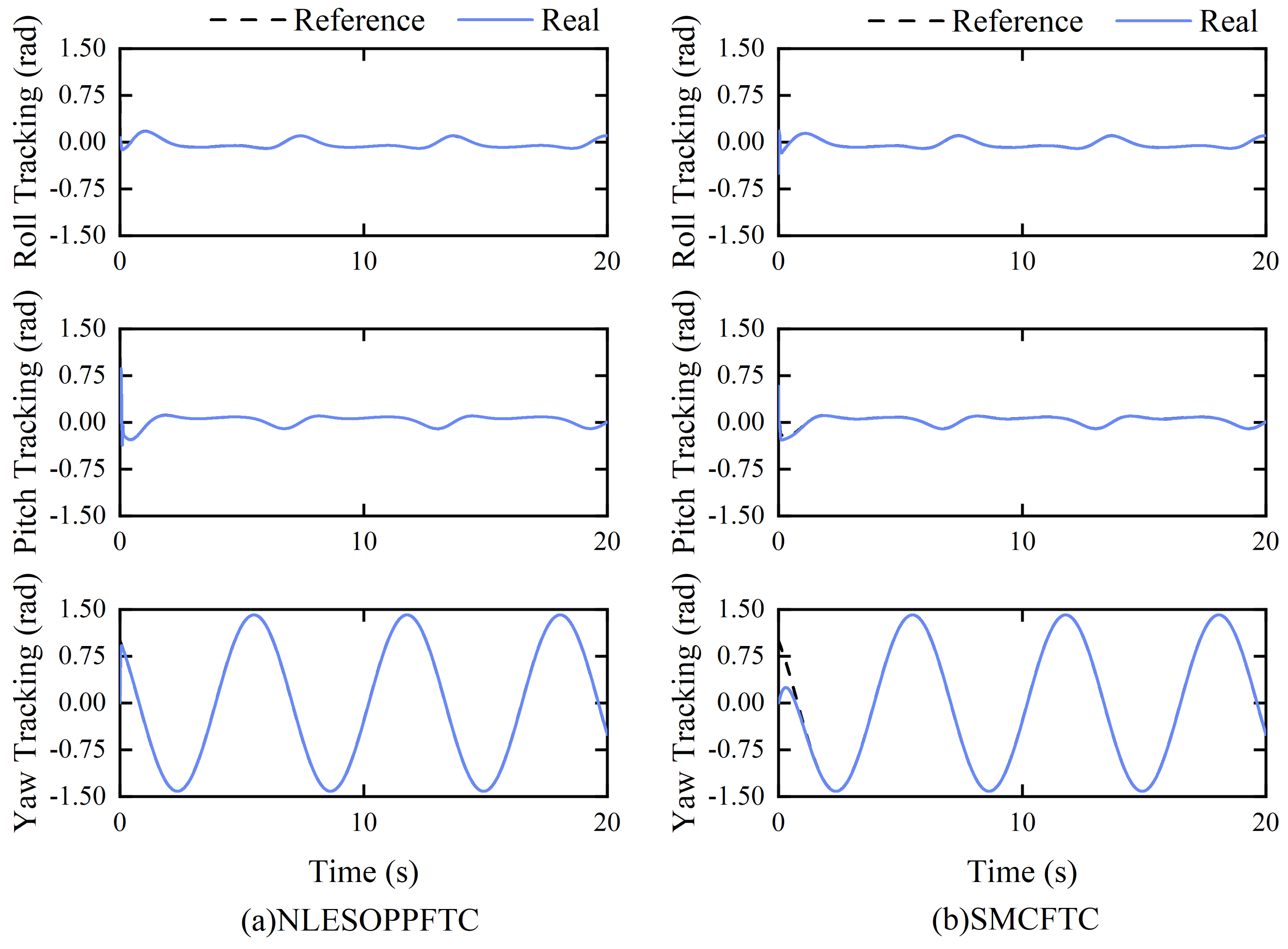
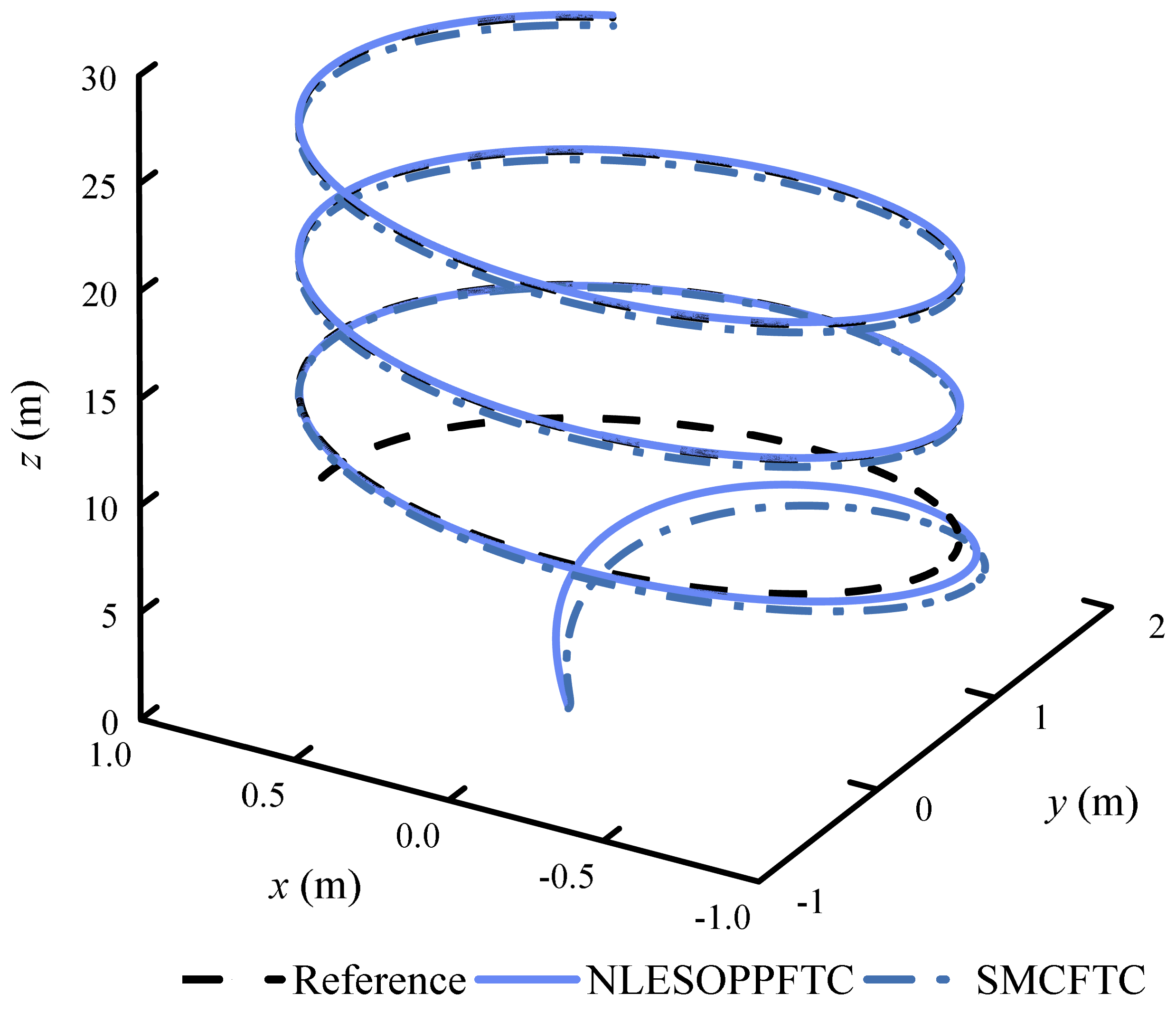
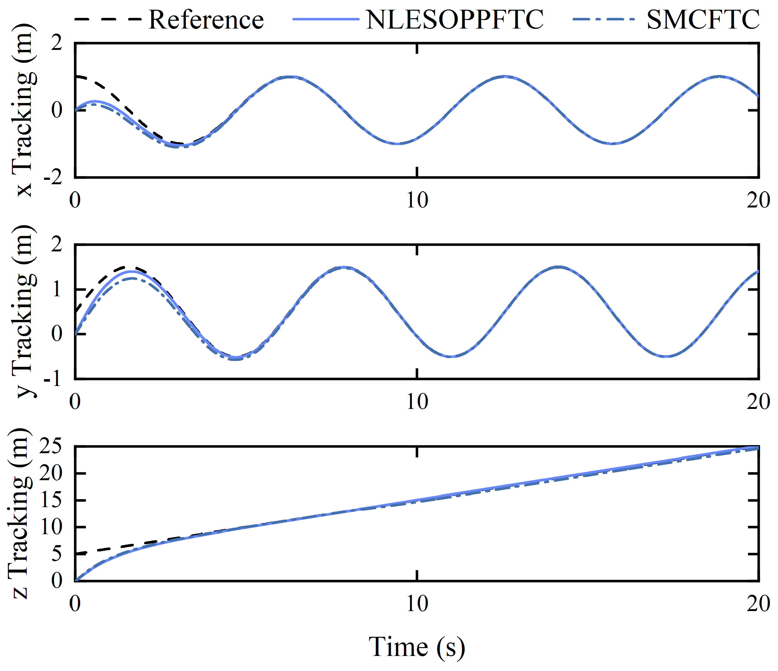
4.1. Case 1: Fault-Free and Disturbance-Free Tracking

In the initial test, our focus was on assessing the performance of NESOPPFTC in tracking the reference signal under fault-free and undisturbed conditions, in comparison with SMCFTC, the corresponding fault parameters are set as follows: ${\tau }_{\mathrm{x}}={\tau }_{\mathrm{y}}={\tau }_{\mathrm{z}}=0$, $u_{xf}=u_{yf}=u_{zf}=0$, ${\tau }_{\varphi }={\tau }_{\theta }={\tau }_{\psi }=0$, and $u_{\varphi f}=u_{\theta f}=u_{\psi f}=0$. The disturbance parameters are configured as follows: $d_3=d_4=d_5=d_6=0$. Figure 3 and Figure 4 demonstrate that NESOPPFTC closely follows the desired trajectory, with a noticeably faster adjustment speed than SMCFTC. Particularly in the control of the yaw channel, as clearly observed in Figure 5, NESOPPFTC is significantly quicker than SMCFTC. This indicates that, although NESOPPFTC is designed as a controller for fault conditions, it still maintains good performance and robustness even in the absence of faults and disturbances.

4.2. Case 2: Constant Fault and Disturbance Tracking

As shown in Figure 6 and Figure 7, the 3D trajectory tracking comparison between the proposed NLESOPPFTC and the conventional sliding mode fault-tolerant control (SMCFTC) is presented. The analysis reveals that NLESOPPFTC achieves superior tracking accuracy and speed compared to the traditional SMC algorithm. Particularly at t = 8 s, NLESOPPFTC demonstrates robust performance in handling faults in the z-channel, whereas SMCFTC exhibits noticeable deficiencies in tracking the desired trajectory when complex faults and external disturbances occur. This is especially evident in the z-channel trajectory tracking, where, despite prolonged dynamic adjustments, significant deviations persist. Figure 8 displays the time response of the state estimation for the proposed control scheme. It can be inferred that NESOPPFTC accurately estimates fault state information and exhibits rapid convergence and high precision, allowing the system to quickly revert to the desired trajectory after disturbances and faults at 8 s. As illustrated by the attitude tracking curves in Figure 9, the NLESOPPFTC scheme significantly outperforms the SMCFTC scheme in terms of attitude tracking. Although the SMCFTC scheme can also converge rapidly to the desired attitude during complex faults, it generates considerable oscillations in the roll and yaw channels due to issues with the switching function in the SMC approach’s sliding law, approaching angles close to a gimbal lock situation, which is unacceptable in practical applications.

To more closely align with real-world engineering applications and further validate the proposed control scheme, Gaussian noise interference was introduced for simulation testing, with a noise power of 0.0005. As depicted in Figure 10, during fault occurrences and with the addition of Gaussian noise, the proposed scheme is able to track the desired angles more accurately compared to the SMCFTC scheme, which exhibits insufficient performance in tracking the desired posture under Gaussian perturbations. Figure 11 presents the error tracking response curves for both the NLESOPPFTC and SMCFTC schemes. It is evident that the control strategy proposed in this paper allows adjustment to the desired posture within a finite time under the influence of the controller, with each position and posture state strictly maintained within the predetermined performance boundaries. In contrast, the state variables of the SMCFTC scheme show a significantly longer convergence time and a persistent steady-state error after extended adjustments. From Figure 11b and the RMSE values of the tracking trajectory after adding Gaussian perturbation and without adding Gaussian perturbation in

Table 2. Comparison of motion tracking RMSE with and without Gaussian noise.

Index		RMSE
NLESOPPFTC	z	0
	$\varphi$	5.11 × 10−2
	$\theta$	5.31 × 10−2
	$\psi$	1.83 × 10−9
SMCFTC	z	1.44 × 10−1
	$\varphi$	7.57 × 10−2
	$\theta$	8.17 × 10−2
	$\psi$	9.84 × 10−3

(RMSE is calculated by normalizing the data to eliminate the effect of magnitude between the metrics), it is clear that the SMCFTC scheme experiences significant fluctuations upon the introduction of Gaussian noise, whereas the NLESOPPFTC is confined within the set performance boundaries. This demonstrates that NLESO possesses excellent noise filtering capabilities, robustness against unknown system states, and PPC provides effective control over both steady-state and dynamic performance.

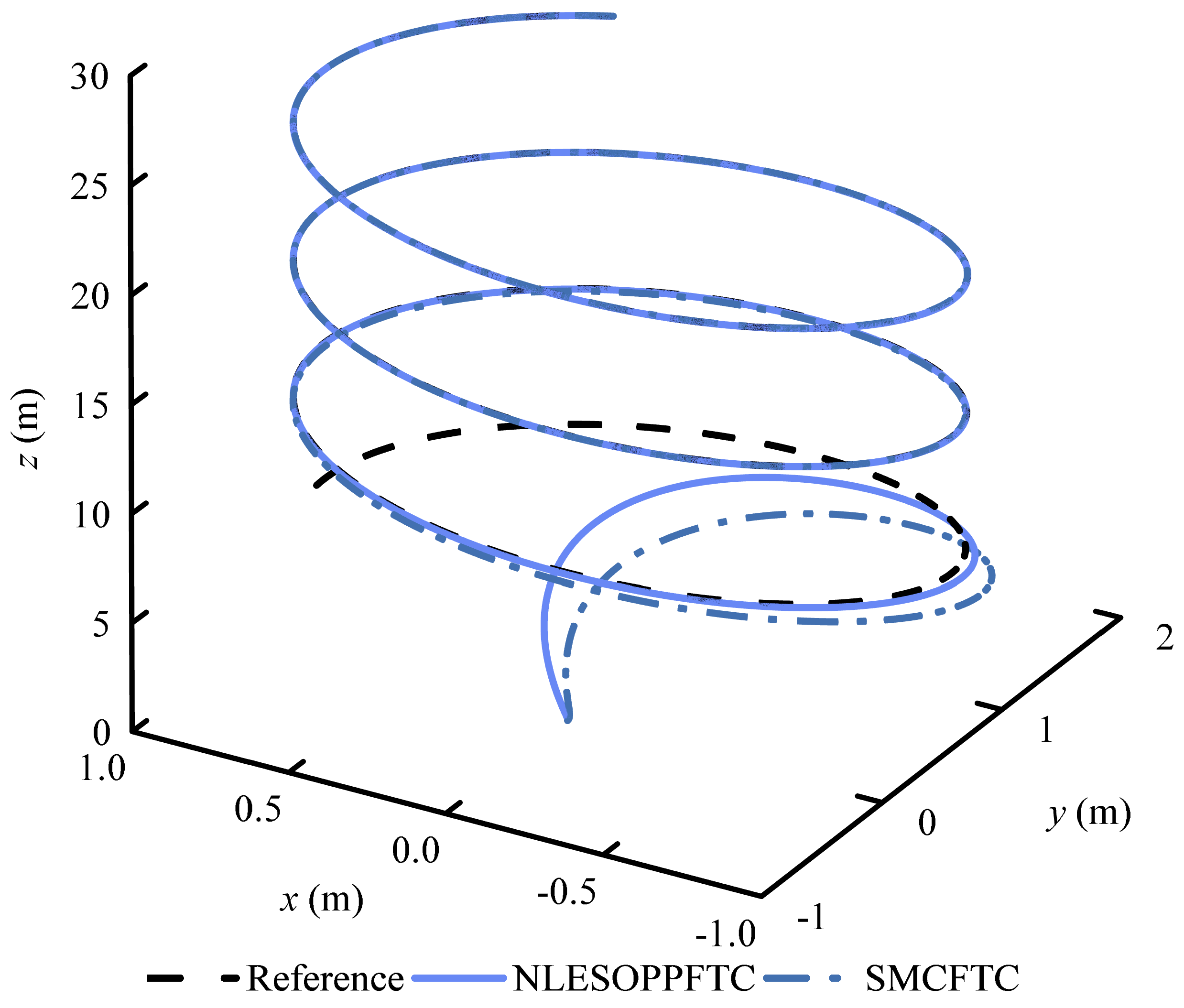
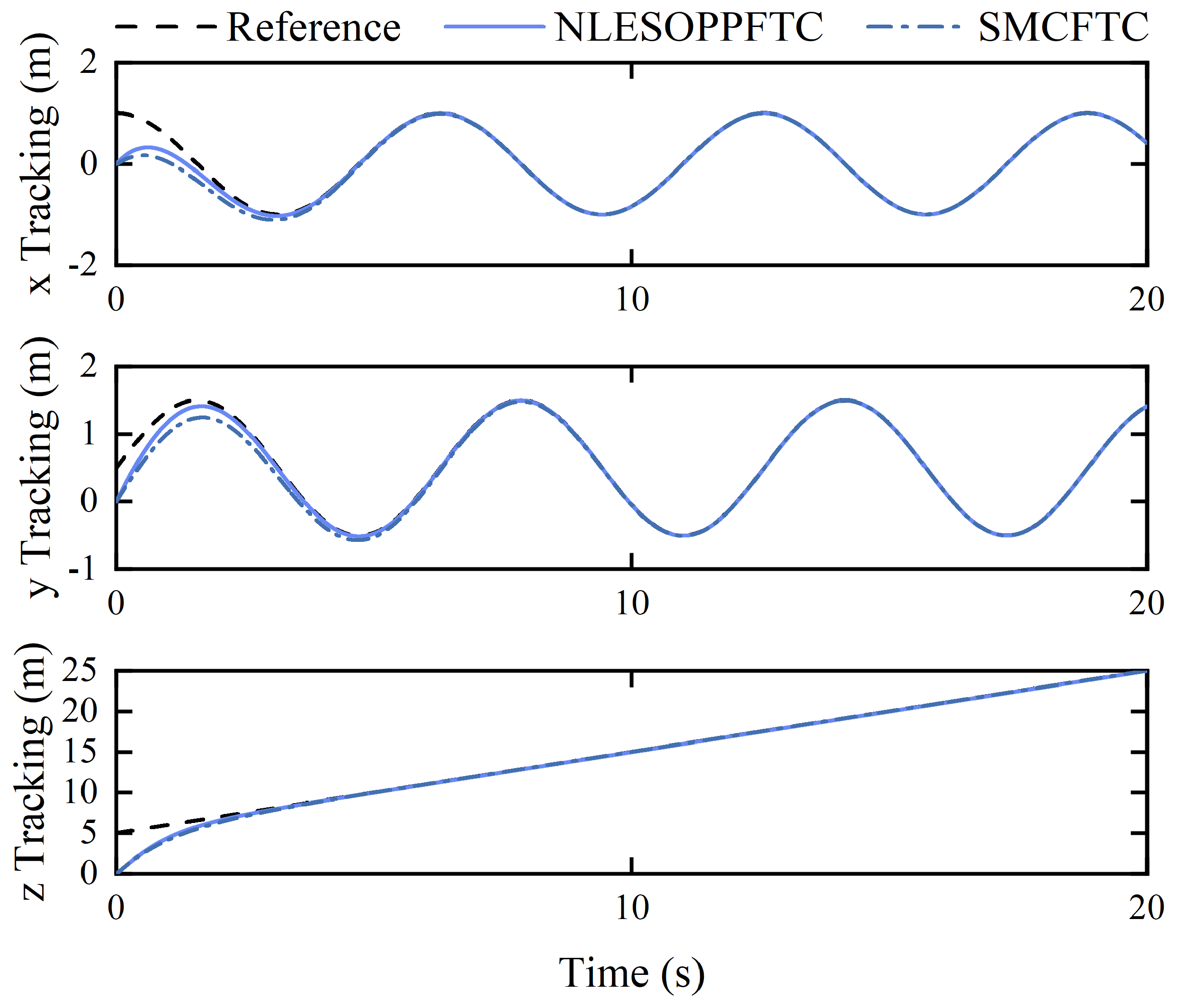
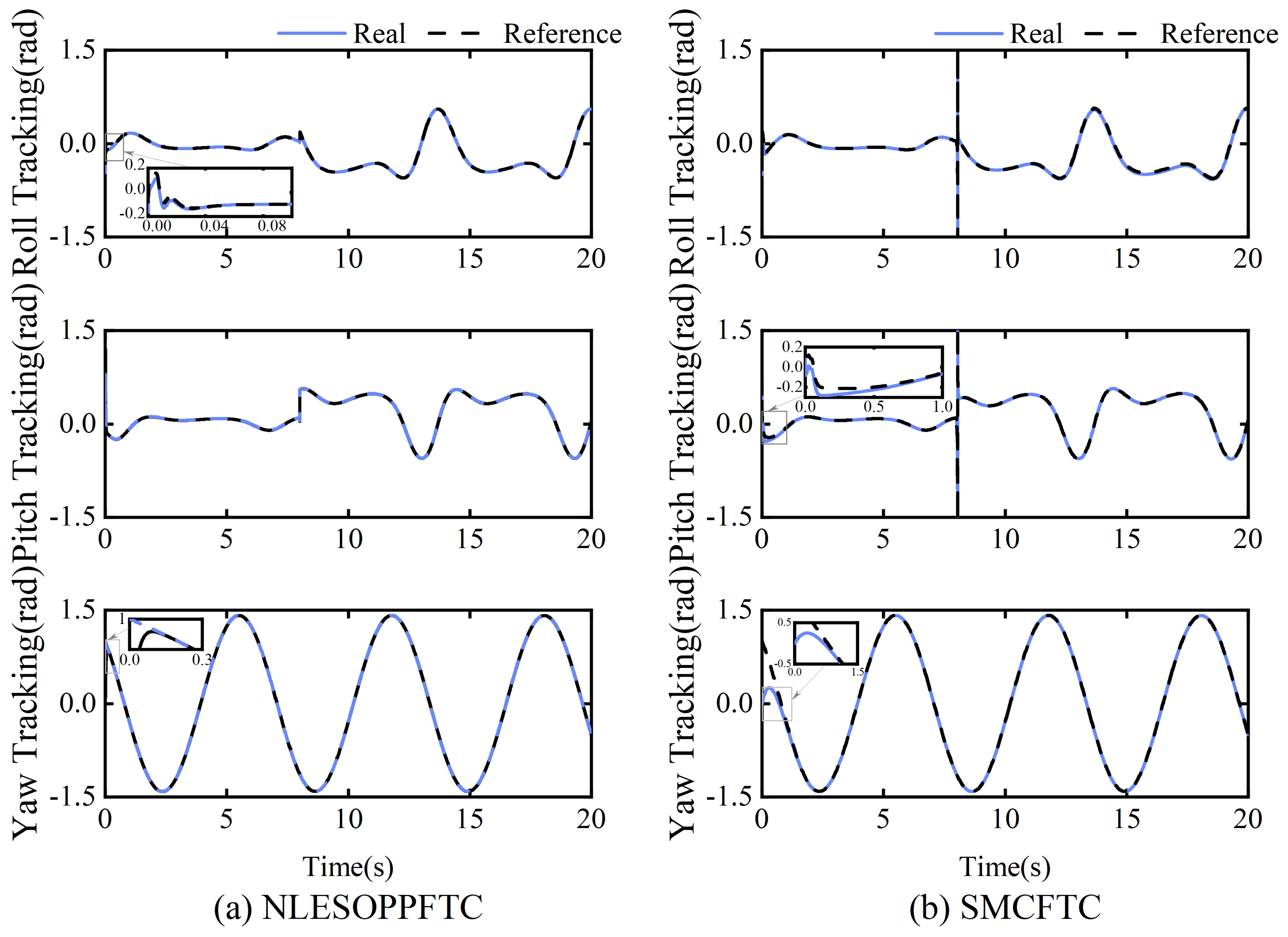
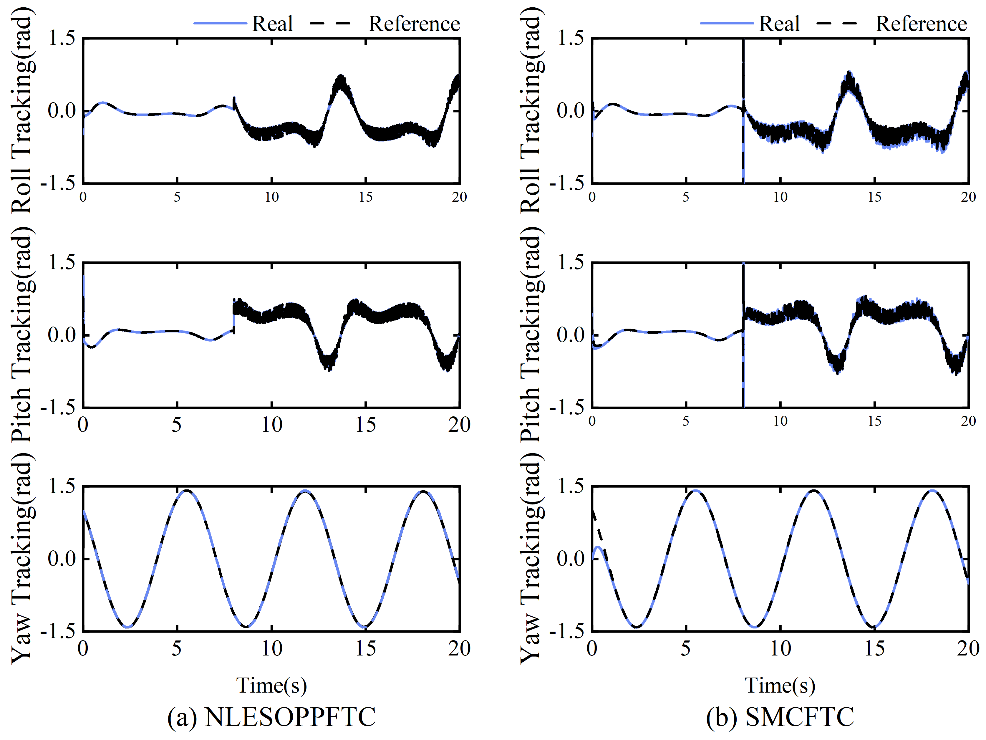
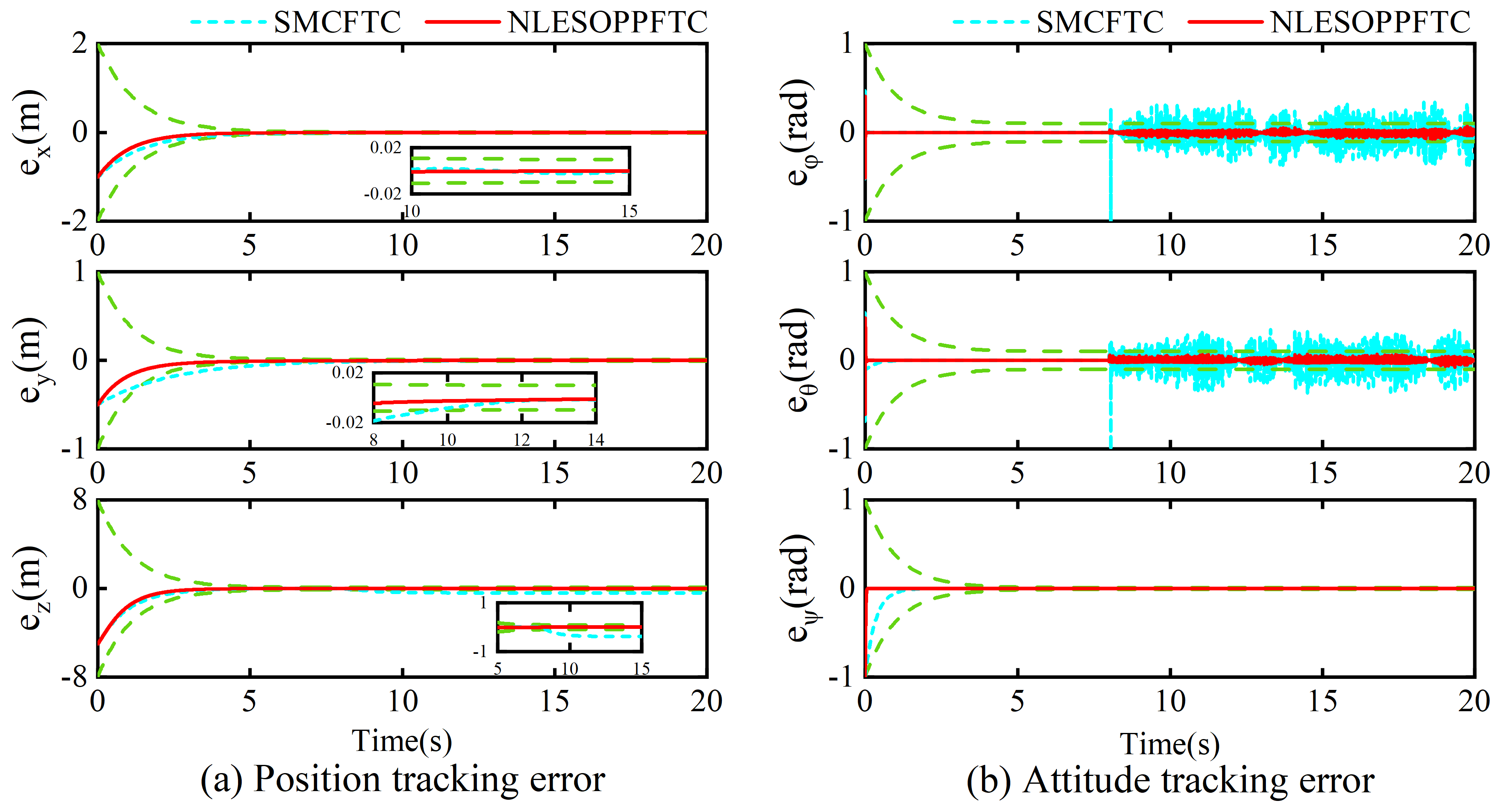
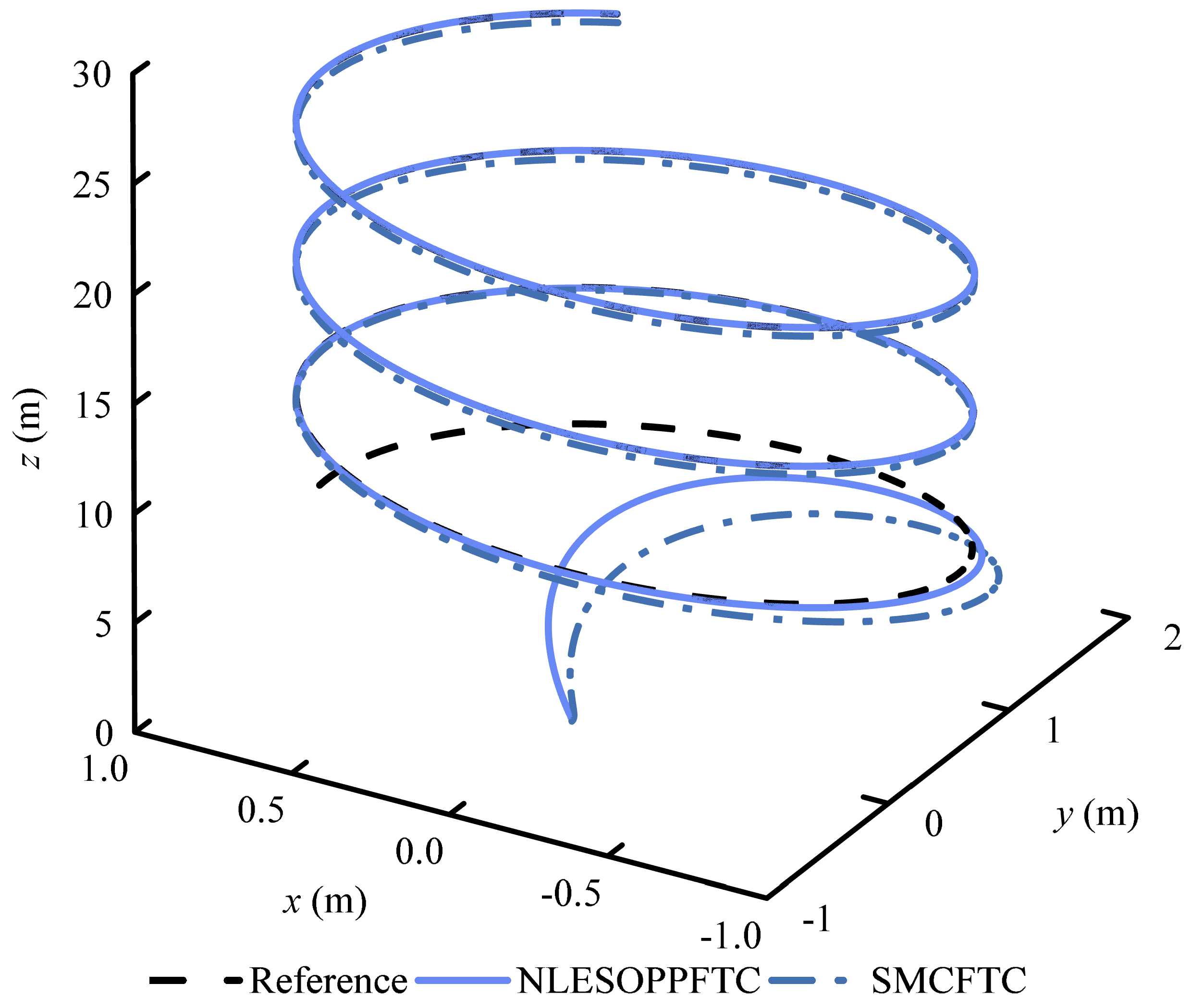
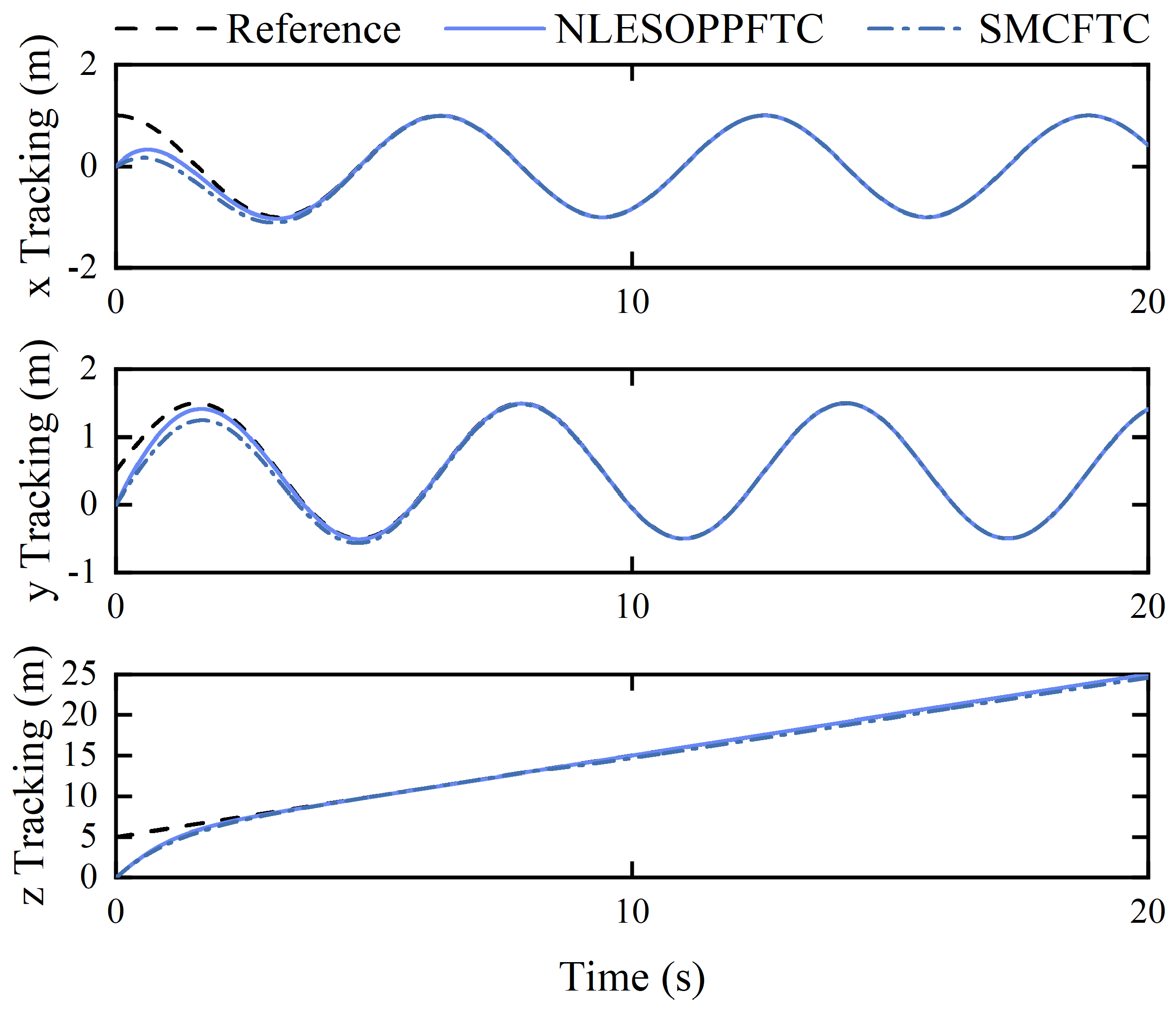
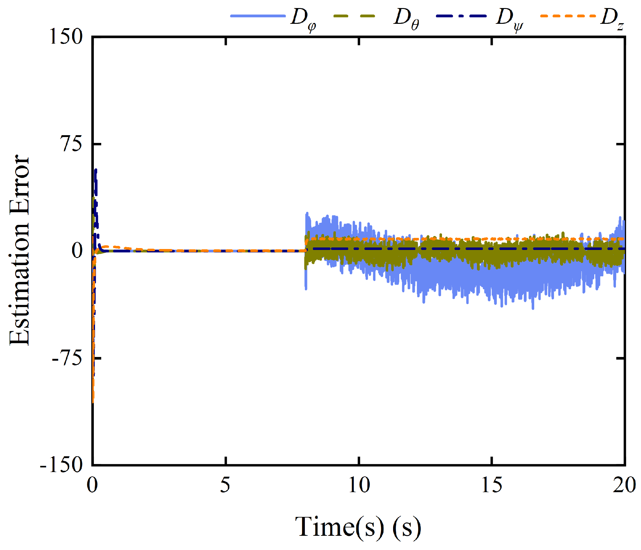
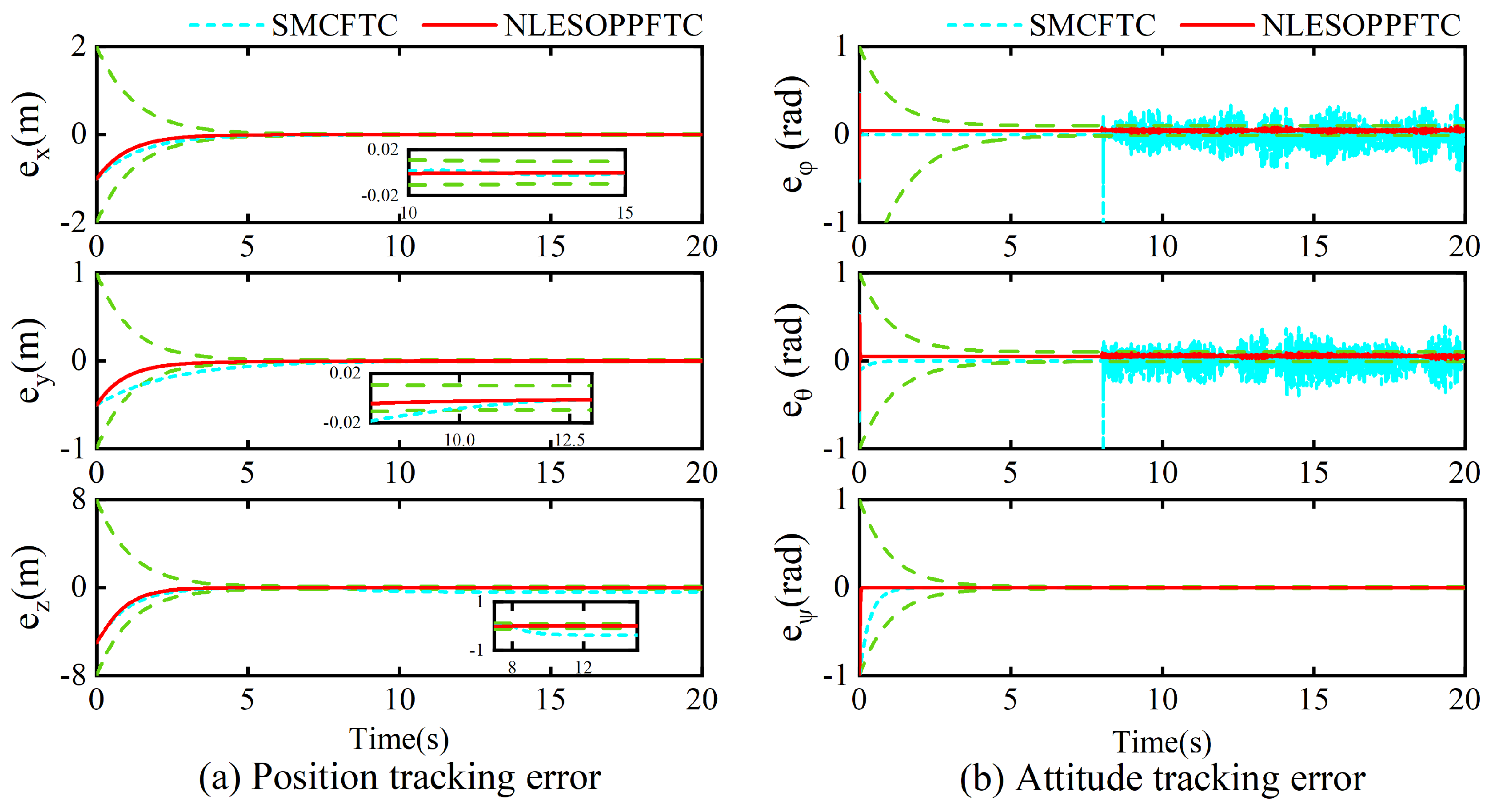
4.3. Case 3: Time-Varying Fault and Disturbance Tracking

In the third test, we focused on evaluating the performance of NESOPPFTC in tracking the reference signal under compound conditions of time-varying faults, bias faults, and noise interference. The fault parameters were set as follows: ${\tau }_{\mathrm{x}}={\tau }_{\mathrm{y}}=0$, ${\tau }_z=0.5+0.2sin\left(t\right)$, $u_{xf}=u_{yf}=0$, $u_{zf}=4$, ${\tau }_{\varphi }={\tau }_{\theta }={\tau }_{\psi }=0.64+0.2sin\left(t\right)$, $u_{\varphi f}=0.1sin\left(0.1\pi t\right)$, and $u_{\theta f}=2$, $u_{\psi f}=3sin\left(0.3\pi t\right)$. The disturbance parameters are configured as follows: $d_3=5$, $d_4=0.5$, $d_5=2sin\left(0.5\pi t\right)$, and $d_6=1.5$.

As illustrated in Figure 12 and Figure 13, the position tracking curves were similar to those in Case 2. However, as observed in Figure 14, the SMCFTC scheme exhibited greater errors compared to Case 2, whereas the performance of NLESOPPFTC was nearly identical. Figure 15 indicates that even in the presence of time-varying faults, the NESOPPFTC scheme could still accurately estimate state information for compensation, achieving rapid convergence with high precision, and allowing the system to quickly return to the desired trajectory. Figure 16 confirms that under these circumstances, the system can still converge to a stable state within a finite time according to the performance boundaries set in PPC, and strictly within these boundaries. Finally, the integral time-weighted absolute error (ITAE) was used as a performance metric to evaluate both schemes, as shown in

Table 3. Evaluation indexes.

Evaluation Indexes		NLESOPPFTC	SMCFTC
ITAE a	x	0.837	2.255
	y	0.810	2.929
	z	5.873	65.690
	$\varphi$	0.434	4.066
	$\theta$	0.690	0.783
	$\psi$	0.028	0.128
Proposed control strategy b	$U_1$	8.524	8.698
	$U_2$	1066	2.527 × 104
	$U_3$	1156	2.264 × 104
	$U_4$	0.488	0.507

^a The ITAE is calculated by a standard measure, denoted as the integral of the product of the absolute value of the error and time [43]. ^b Energy consumption is calculated by a standard measure, denoted as the integration of the absolute of control input [44].

, where NLESOPPFTC’s ITAE value was significantly lower than that of SMCFTC, also demonstrating the superiority of the control algorithm proposed in this paper.

Given that drone control systems in practical applications benefit from simpler, more computationally efficient controllers, the operational time of the control algorithms tested showed that the response time for NLESOPPFTC was 7 ms, compared to 5 ms for SMCFTC. Although the response time was longer than that of SMCFTC, it remained within acceptable limits. Additionally, as indicated in Table 3, the energy consumption, especially in channels $U_2$ and $U_3$, required significantly fewer data updates, which is beneficial for rapid data transmission in practical applications. In conclusion, the use of NLESOPPFTC demonstrated excellent noise filtering capabilities, robustness to unknown system states, and PPC showed effective control of steady-state and dynamic performances, underscoring the stability designed in this study and its feasibility for practical applications.

5. Conclusions

In the context of quadrotor UAVs executing tasks amidst unknown disturbances and composite faults, nonlinear extended state observer and prescribed performance fault-tolerant control is proposed. This control scheme ensures the stability of the control system within a finite time and enables the system to converge within a predefined performance curve. NLESO is designed based on the system’s fault model, estimating both system faults and uncertain states, then compensating for these effects within the system. Rigorous stability analysis was conducted to ensure the observer’s stability. Based on NLESO, a full-loop rapid non-singular terminal sliding mode surface is utilized, along with a prescribed performance scheme to design the UAV’s inner and outer loop controllers. This provides attitude and position tracking control and allows for adjustment of the convergence range as needed while offering additional robustness. To verify the effectiveness of this method, simulations were first conducted in the absence of faults to ensure stable operation under fault-free conditions. Further simulations were then performed in the presence of composite faults and disturbances to confirm that the proposed method could still operate stably under these challenging conditions, thereby demonstrating the robustness of the approach outlined in the article. Additionally, compared to traditional sliding mode control, this method achieves higher control precision, faster convergence speeds, and robustness against composite faults and disturbances.

The proposed improvements optimize the operational performance of quadrotor UAVs when facing complex challenges and provide substantial theoretical support and practical guidance for future UAV control system design and optimization. Future efforts may concentrate on adjusting system control parameters for diverse unknown environments and fault scenarios to improve the robustness and adaptability of the proposed control scheme. Additionally, the control strategy could be expanded to include full-attitude trajectory and attitude tracking for quadrotor UAVs, avoiding the gimbal lock issues present in current approaches and facilitating isolated modeling and analysis of single or multiple motor failures.

References

1. Fan, B.; Li, Y.; Zhang, R.; Fu, Q. Review on the Technological Development and Application of UAV Systems. Chin. J. Electron. 2020, 29, 199–207. [Google Scholar] [CrossRef]
2. Nawaz, H.; Ali, H.M.; Laghari, A.A. UAV communication networks issues: A review. Arch. Comput. Methods Eng. 2021, 28, 1349–1369. [Google Scholar] [CrossRef]
3. Khattab, A.; Mizrak, I.; Alwi, H. Fault tolerant control of an octorotor UAV using sliding mode for applications in challenging environments. Annu. Rev. Control 2024, 57, 100952. [Google Scholar] [CrossRef]
4. Zhao, Z.h.; Xiao, L.; Jiang, B.; Cao, D. Fast nonsingular terminal sliding mode trajectory tracking control of a quadrotor UAV based on extended state observers. Control Decis. 2022, 37, 2201–2210. [Google Scholar] [CrossRef]
5. Hu, F.; Ma, T.; Su, X. Adaptive Fuzzy Sliding Mode Fixed-Time Control for Quadrotor Unmanned Aerial Vehicles with Prescribed Performance. IEEE Trans. Fuzzy Syst. 2024, 32, 4109–4120. [Google Scholar] [CrossRef]
6. Wen, G.; Yu, D.; Zhao, Y. Optimized Fuzzy Attitude Control of Quadrotor Unmanned Aerial Vehicle Using Adaptive Reinforcement Learning Strategy. IEEE Trans. Aerosp. Electron. Syst. 2024, 60, 6075–6083. [Google Scholar] [CrossRef]
7. Chen, C.; Zhang, X.; Peng, X. Trajectory tracking control of four-rotor UAV based on nonlinear extended state observer and model predictive control in wind disturbance environment. J. Phys. Conf. Ser. 2024, 2764, 012075. [Google Scholar] [CrossRef]
8. Derakhshan, R.E.; Danesh, M.; Moosavi, H. Disturbance observer-based model predictive control of a coaxial octorotor with variable centre of gravity. IET Control Theory Appl. 2024, 18, 764–783. [Google Scholar] [CrossRef]
9. Chen, H.; Li, J.; Wang, A.; Zhang, Y.; Liang, H. Fault-tolerant control of quadrotor UAV attitude system with actuator failure. Flight Dyn. 2024, 42, 52–59. [Google Scholar]
10. Wang, A.; Li, J.; Xia, G.; Chen, H. Quad-rotor Unmanned Helicopter Presets Performance Adaptive PID Control. Control Eng. China 2024, 31, 865–875. [Google Scholar]
11. Jin, P.; Ma, Q.; Xu, S. Dynamic Event-Triggered Robust Optimal Attitude Control of QUAV Using Reinforcement Learning. IEEE Trans. Aerosp. Electron. Syst. 2023, 59, 7798–7807. [Google Scholar] [CrossRef]
12. Yan, K.; Zhang, J.R.; Ren, H.P. Interval Observer-based Robust Trajectory Tracking Control for Quadrotor Unmanned Aerial Vehicle. Int. J. Control. Autom. Syst. 2024, 22, 288–300. [Google Scholar] [CrossRef]
13. Xu, S.; Huang, W.; Wang, H.; Zheng, W.; Wang, J.; Chai, Y.; Ma, M. A Simultaneous Diagnosis Method for Power Switch and Current Sensor Faults in Grid-Connected Three-Level NPC Inverters. IEEE Trans. Power Electron. 2023, 38, 1104–1118. [Google Scholar] [CrossRef]
14. Xie, D.; Lin, C.; Deng, Q.; Lin, H.; Cai, C.; Basler, T.; Ge, X. Simple Vector Calculation and Constraint-Based Fault-Tolerant Control for a Single-Phase CHBMC. IEEE Trans. Power Electron. 2024, 1–14. [Google Scholar] [CrossRef]
15. Abushafa, O.S.H.M.; Dahidah, M.S.A.; Gadoue, S.M.; Atkinson, D.J. Submodule Voltage Estimation Scheme in Modular Multilevel Converters with Reduced Voltage Sensors Based on Kalman Filter Approach. IEEE Trans. Ind. Electron. 2018, 65, 7025–7035. [Google Scholar] [CrossRef]
16. Niederlinski, A. A heuristic approach to the design of linear multivariable interacting control systems. Automatica 1971, 7, 691–701. [Google Scholar] [CrossRef]
17. Gong, W.; Li, B.; Yang, Y.; Ban, H.; Xiao, B. Fixed-time integral-type sliding mode control for the quadrotor UAV attitude stabilization under actuator failures. Aerosp. Sci. Technol. 2019, 95, 105444. [Google Scholar] [CrossRef]
18. Abbaspour, A.; Mokhtari, S.; Sargolzaei, A.; Yen, K.K. A Survey on Active Fault-Tolerant Control Systems. Electronics 2020, 9, 1513. [Google Scholar] [CrossRef]
19. Yang, S.; Zou, Z.; Li, Y.; Shi, H.; Fu, Q. Adaptive Fault-Tolerant Tracking Control of Quadrotor UAVs against Uncertainties of Inertial Matrices and State Constraints. Drones 2023, 7, 107. [Google Scholar] [CrossRef]
20. Liu, H.; Tu, H.; Huang, S.; Zheng, X. Adaptive Predefined-Time Sliding Mode Control for QUADROTOR Formation with Obstacle and Inter-Quadrotor Avoidance. Sensors 2023, 23, 2392. [Google Scholar] [CrossRef]
21. Jung, W.; Bang, H. Fault and Failure Tolerant Model Predictive Control of Quadrotor UAV. Int. J. Aeronaut. Space Sci. 2021, 22, 663–675. [Google Scholar] [CrossRef]
22. Cui, G.; Yang, W.; Yu, J. Neural network-based finite-time adaptive tracking control of nonstrict-feedback nonlinear systems with actuator failures. Inf. Sci. 2021, 545, 298–311. [Google Scholar] [CrossRef]
23. Brahim, K.S.; Hajjaji, A.E.; Terki, N.; Alabazares, D.L. Finite Time Adaptive SMC for UAV Trajectory Tracking Under Unknown Disturbances and Actuators Constraints. IEEE Access 2023, 11, 66177–66193. [Google Scholar] [CrossRef]
24. Prochazka, K.F.; Stomberg, G. Integral Sliding Mode based Model Reference FTC of an Over-Actuated Hybrid UAV using Online Control Allocation. In Proceedings of the 2020 American Control Conference (ACC), Denver, CO, USA, 1–3 July 2020; pp. 3858–3864. [Google Scholar] [CrossRef]
25. Karahan, M.; Inal, M.; Kasnakoglu, C. Fault Tolerant Super Twisting Sliding Mode Control of a Quadrotor UAV Using Control Allocation. Int. J. Robot. Control Syst. 2023, 3, 270–285. [Google Scholar] [CrossRef]
26. Nan, F.; Sun, S.; Foehn, P.; Scaramuzza, D. Nonlinear MPC for Quadrotor Fault-Tolerant Control. IEEE Robot. Autom. Lett. 2022, 7, 5047–5054. [Google Scholar] [CrossRef]
27. Yang, P.; Wang, Z.; Zhang, Z.; Hu, X. Sliding Mode Fault Tolerant Control for a Quadrotor with Varying Load and Actuator Fault. Actuators 2021, 10, 323. [Google Scholar] [CrossRef]
28. Dou, J.; Kong, X.; Wen, B. Backstepping Sliding Mode Active Disturbance Rejection Control of Quadrotor Attitude and Its Stability. J. Northeast. Univ. (Nat. Sci.) 2016, 37, 1415–1420. [Google Scholar] [CrossRef]
29. He, D.; Wang, H.; Tian, Y. Model-Free Control Using Nonlinear Extended State Observer and Non-singular Fast Terminal Sliding Mode for Quadrotor Position and Attitude. In Proceedings of the 2020 39th Chinese Control Conference (CCC), Shenyang, China, 27–29 July 2020; pp. 1891–1896. [Google Scholar] [CrossRef]
30. Bechlioulis, C.P.; Rovithakis, G.A. Robust Adaptive Control of Feedback Linearizable MIMO Nonlinear Systems with Prescribed Performance. IEEE Trans. Autom. Control 2008, 53, 2090–2099. [Google Scholar] [CrossRef]
31. Pan, S.; Jiang, B.; Zhu, R.; Yin, X. Prescribed Performance Back-stepping Control of Fast Trajectory Tracking for Quad-rotor Aircraft. Control Eng. China 2021, 28, 2199–2208. [Google Scholar] [CrossRef]
32. Gong, W.; Li, B.; Ahn, C.K.; Yang, Y. Prescribed-time extended state observer and prescribed performance control of quadrotor UAVs against actuator faults. Aerosp. Sci. Technol. 2023, 138, 108322. [Google Scholar] [CrossRef]
33. Hu, Y.; Zhang, L.; Geng, B. Research Development of Prescribed Performance Control. J. Nav. Aeronaut. Astronaut. Univ. 2016, 31, 1–6. [Google Scholar] [CrossRef]
34. Zhou, L.; Liu, H.; Li, X. Active disturbance rejection preset finite-time control for a UAV with unknown initial tracking condition. J. Univ. Sci. Technol. Liaoning 2023, 46, 111–119. [Google Scholar]
35. Zhu, W.; Wang, C.; Deng, W.; Liang, X.; Yao, J. Nonsingular Terminal Sliding Mode Based Prescribed Performance Control of Motor Servo Systems. J. Mech. Eng. 2023, 59, 359–366. [Google Scholar]
36. Li, H.; Wei, J.; Fang, D.; Li, J. Prescribed performance control for hypersonic vehicle considering input constraint. J. Natl. Univ. Def. Technol. 2023, 45, 27–36. [Google Scholar] [CrossRef]
37. Wang, L.; Pei, H.; Cheng, Z. Geometric Attitude Fault-Tolerant Control of Quadrotor Unmanned Aerial Vehicles with Adaptive Extended State Observers. Machines 2024, 12, 47. [Google Scholar] [CrossRef]
38. Liu, J.; Tan, J.; Pu, M.; Zhang, G.; Dan, Z.; Guo, G. Novel third-order fixed-time convergent nonlinear extended state observer based on sliding mode control method. Control Decis. 2024. [Google Scholar] [CrossRef]
39. Hasan, A.; Johansen, T.A. Model-based actuator fault diagnosis in multirotor UAVs. In Proceedings of the 2018 International Conference on Unmanned Aircraft Systems (ICUAS), Dallas, TX, USA, 12–15 June 2018; pp. 1017–1024. [Google Scholar]
40. Zhang, S.; Wu, H.; Zheng, X. Finite-time fault tolerant control of quadrotor UAV with actuator faults. Control Theory Appl. 2023, 40, 1270–1276. [Google Scholar]
41. Asadi, D. Model-based Fault Detection and Identification of a Quadrotor with Rotor Fault. Int. J. Aeronaut. Space Sci. 2022, 23, 916–928. [Google Scholar] [CrossRef]
42. Yu, S.; Yu, X.; Shirinzadeh, B.; Man, Z. Continuous finite-time control for robotic manipulators with terminal sliding mode. Automatica 2005, 41, 1957–1964. [Google Scholar] [CrossRef]
43. Yin, C.; Wang, S.; Gao, J. A unified design approach for control integrating processes with time delay. PLoS ONE 2024, 19, e0299893. [Google Scholar] [CrossRef]
44. Shao, X.; Xu, L.; Zhang, W. Quantized Control Capable of Appointed-Time Performances for Quadrotor Attitude Tracking: Experimental Validation. IEEE Trans. Ind. Electron. 2022, 69, 5100–5110. [Google Scholar] [CrossRef]
Figure 1. Schematic diagram of a quadrotor UAV.
Aerospace 11 00903 g001
Figure 2. Control architecture: the green dashed arrow represent fault status inputs.
Aerospace 11 00903 g002
Figure 3. 3D trajectory under fault-free and disturbance-free tracking.
Aerospace 11 00903 g003
Figure 4. Position tracking curve under fault-Free and disturbance-free tracking.
Aerospace 11 00903 g004
Figure 5. Estimation error under fault-free and disturbance-free tracking.
Aerospace 11 00903 g005
Figure 6. 3D trajectory under constant fault and disturbance tracking.
Aerospace 11 00903 g006
Figure 7. Position tracking curve under constant fault and disturbance tracking.
Aerospace 11 00903 g007
Figure 8. Estimation error under constant fault and disturbance tracking.
Aerospace 11 00903 g008
Figure 9. Attitude tracking curve under constant fault and disturbance tracking.
Aerospace 11 00903 g009
Figure 10. Attitude tracking curve with Gaussian noise introduced under constant fault and disturbance tracking.
Aerospace 11 00903 g010
Figure 11. Position and attitude tracking error: the green dashed line indicates the upper and lower bounds of the preset performance function of PPC.
Aerospace 11 00903 g011
Figure 12. 3D trajectoryunder time-varying fault and disturbance tracking.
Aerospace 11 00903 g012
Figure 13. Position tracking curve under time-varying fault and disturbance tracking.
Aerospace 11 00903 g013
Figure 14. Attitude tracking curve under time-varying fault and disturbance tracking.
Aerospace 11 00903 g014
Figure 15. Estimation error under time-varying fault and disturbance tracking.
Aerospace 11 00903 g015
Figure 16. Attitude tracking curve with Gaussian noise introduced: the green dashed line indicates the upper and lower bounds of the preset performance function of PP.
Aerospace 11 00903 g016