A Physics- and Data-Driven Study on the Ground Effect on the Propulsive Performance of Tandem Flapping Wings

Abstract

In this paper, we present a physics- and data-driven study on the ground effect on the propulsive performance of tandem flapping wings. With numerical simulations, the impact of the ground effect on the aerodynamic force, energy consumption, and efficiency is analyzed, revealing a unique coupling effect between the ground effect and the wing–wing interference. It is found that, for smaller phase differences between the front and rear wings, the thrust is higher, and the boosting effect due to the ground on the rear wing (maximum of 12.33%) is lower than that on a single wing (maximum of 43.83%) For a larger phase difference, a lower thrust is observed, and it is also found that the boosting effect on the rear wing is above that on a single wing. Further, based on the bidirectional gate recurrent units (BiGRUs) time-series neural network, a surrogate model is further developed to predict the unsteady aerodynamic characteristics of tandem flapping wings under the ground effect. The surrogate model exhibits high predictive precision for aerodynamic forces, energy consumption, and efficiency. On the test set, the relative errors of the time-averaged values range from −4% to 2%, while the root mean squared error of the transient values is less than 0.1. Meanwhile, it should be pointed out that the established surrogate model also demonstrates strong generalization capability. The findings contribute to a comprehensive understanding of the ground effect mechanism and provide valuable insights for the aerodynamic design of tandem flapping-wing air vehicles operating near the ground.

1. Introduction

In nature, insects and birds often use flapping wings to achieve flexible and efficient movements, and the aerodynamic characteristics of flapping wings have also become an active research topic [1,2,3,4,5,6,7,8,9,10]. When insects skim the ground, the ground will have a significant impact on the aerodynamic performance of the insects, which is called the ground effect [11]. At present, the study of the ground effect mainly includes two types of motion: hovering and forward flight.

Research on the ground effect has mainly focused on the hovering mode. In 2008, Gao and Lu [11], employing the Immersion Boundary-Lattice Boltzmann Method (IB-LBM), studied the ground effect of insects in the normal-hovering mode. They analyzed the ground effect on aerodynamic force and vortex structure and revealed the mechanism of force enhancement, force reduction, and force recovery, which was later confirmed by Lua et al. [12] in 2014 by digital particle image velocimetry (DPIV) experiments. Maeda et al. [13] used 3D computational fluid dynamics (CFD) simulations to study the aerodynamic performance of Drosophila in terms of the in-ground effect (IGE) and off-ground effect (OGE) and found that high frequency and low ground clearance are beneficial to the generation of thrusts and large lifts. In 2018, Umar and Sun [14] discovered that the ground effect of hovering rectangular wings resulted in an increase in lift and a decrease in power within a height h of 2.5c (c is the chord length of the flapping wing). Zheng et al. [15] also adopted h/c = 2.5 as the demarcation height and delineated it into the ground effect zone and the transition zone. Meng et al. [16,17,18] conducted numerical simulations to investigate the ceiling effect and ground effect of a three-dimensional hovering flapping wing at low Reynolds number of Re = 10, revealing a coupling effect between the ground effect and the ceiling effect. During hovering, in addition to the ground effect, the impact of local barriers or obstructions on aerodynamic characteristics is also a matter of concern. Wang et al. [19] discovered that the average lift of a two-dimensional elliptical airfoil in hovering is closely correlated with the ground clearance and the horizontal distance from the edge. Bo et al. [20] investigated the effect of obstacle size on the aerodynamic performance of hovering flapping wings.

Compared to the studies on hovering, current studies on the ground effect during forward flight are still limited. Wu et al. [21] examined the ground effect of the NACA0012 airfoil in close proximity to the ground under Re = 150 in 2013. It is indicated that a high Strouhal number and a short distance are advantageous for producing both thrust and lift. In 2014, Wu et al. [22] used an IB-LBM to study the flow characteristics of the NACA0012 airfoil close to the ground under the combined action of harmonic dive and pitch rotation. Mivehchi et al. [23] conducted underwater experiments and found that the ground clearance significantly affects the time-averaged thrust and lift of the flapping wing under propulsion mode. They also discussed the 3D effects at the wing tips and the influence of the spanwise flow on the wing surface. Lin et al. [24] studied the asymmetric lift and sink motion modes under the ground effect and found that a shorter upstroke time is conducive to generating higher thrust, while a shorter downstroke time is conducive to generating lift. In 2021, Li et al. [25] studied the impact of ground effects on the flapping wing propulsion performance at a relatively high Reynolds number (Re = 10⁴) through numerical simulations. Most recently in 2024, Lin et al. [26] numerically considered the effect of the existence of a boundary layer on the aerodynamic forces and the vortex evolution dynamics in the wake. However, these previous studies have primarily focused on single wings, with limited research conducted on the ground effects of tandem wings.

In nature, many insects with exceptional flying abilities, such as dragonflies, are equipped with tandem wings. In comparison to a single pair of wings, tandem wings can generally obtain greater lift and propulsion, resulting in improved propulsion efficiency in specific trajectories and environments [27,28,29,30,31,32]. Srinidhi et al. [33] studied the ground effect of tandem flapping wings hovering on an inclined stroke plane. They discovered that the in-phase stroking can generate the greatest vertical force, while counter-stroking can enhance body stability. Zheng et al. [15] also studied the ground effect of tandem wings hovering on the inclined stroke plane and described the influence of ground effect on the trajectory of shedding vortex. So far, there has been little research available on the ground effect of tandem wings in the forward flight mode.

Therefore, in this study, numerical simulations are carried out to investigate the ground effect on the hydrodynamic behaviors of tandem wings in the forward flight mode. Furthermore, utilizing the deep learning framework of PyTorch, a time-series neural network model centered on bidirectional gated recurrent units (BiGRUs) [34] is established to predict the aerodynamic performance of tandem wings with the ground effect. Through the analysis of the numerical results, the interaction between the ground effect and the wing–wake interaction is examined. This work is anticipated to offer reference for the aerodynamic design of tandem flapping-wing air vehicles operating near the ground.

The paper is outlined as follows. The physical problem, the corresponding numerical method and its validations are presented in Section 2, including the neural network modeling. In Section 3, we first discuss the numerical results of the propulsive performance from the perspective of the vortex structure evolution, and then the prediction of the aerodynamic performance by the surrogate model is presented. In the end, we summarize the main results in Section 4.

2. Materials and Methods

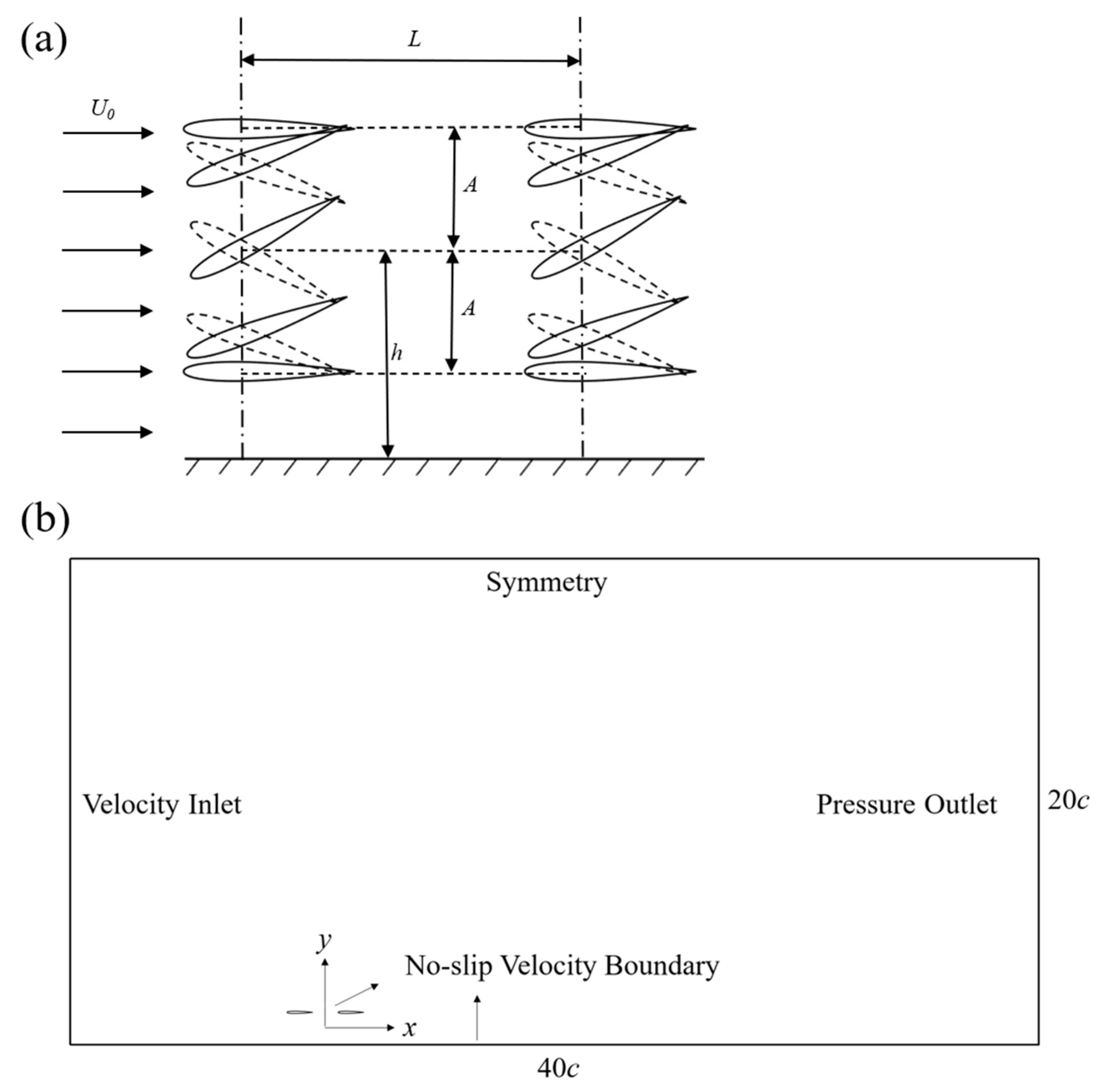
2.1. Physical Problem and Numerical Model

A two-dimensional simplified diagram of the tandem wing in the forward flight mode is shown in Figure 1a. Two wings are in a parallel free flow, and their motion is composed of simple pitching motion and heaving motion, governed by the following equations:

$$\begin{array}{l}{y}_{\mathrm{F}}=A\cos (2\pi ft),\hfill \\ {\alpha }_{\mathrm{F}}={\alpha }_0\cos (2\pi ft+\pi /2),\hfill \\ y_{\mathrm{R}}=A\cos (2\pi ft+\phi ),\hfill \\ {\alpha }_{\mathrm{R}}={\alpha }_0\cos (2\pi ft+\pi /2+\phi ),\hfill \end{array}$$

(1)

where $y_{\mathrm{F}}$, ${\alpha }_{\mathrm{F}}$, $y_{\mathrm{R}}$, and ${\alpha }_{\mathrm{R}}$ represent the vertical displacement of the front wing, the rotation angle of the front wing, the vertical movement of the rear wing, and the rotation angle of the rear wing, respectively. There is also a phase difference of $\pi /2$ between the pitching motion and heave motion. f is the motion frequency and $\phi$ represents the phase difference between the front and rear wings. The amplitude of the heave motion is set to A = 0.75c, and the amplitude of the pitching motion is ${\alpha }_0$ = 30°. A user-defined function (UDF) following Equation (1) is implemented to realize the wing motion in the present numerical simulations. The computational domain is specified in terms of the chord, as in Figure 1b, with the conditions at all boundaries indicated. And the origin of the coordinates lies at the midpoint between the front and rear wings, which is 10 c from the left boundary of the computational domain.

The wings are subjected to a horizontal fluid flow, with an incoming velocity of U₀ = 0.5 m/s. The chord length of the airfoil is c = 0.01 m and the distance between the front and rear wings is L = 2c. The Strouhal number is set to St = 0.3 because the Strouhal numbers of insects and birds are usually between 0.2 and 0.4 [35]. The dimensionless ground clearance h/c is selected from a range of 0.875 to 5, which describes the distance between the center of the vertical motion of the wing and the ground. When h/c = 0.875, the wings almost touch the ground. The incoming fluid flow is characterized by the Reynolds number, which is defined as

$$Re={\displaystyle \frac{\rho U_{\infty }c}{\mu }},$$

(2)

where $\rho$ is the fluid density, $U_{\infty }$ is the reference velocity, c is the chord length of the wing, and $\mu$ is the dynamic viscosity of the fluid. In this study, Re is set to 1000 for all simulations. Accordingly, the 2D incompressible Navier–Stokes equations needs to be numerically solved to determine the velocity field and, subsequently, the aerodynamic force:

$$\begin{array}{c}{\displaystyle \frac{\partial u}{\partial x}}+{\displaystyle \frac{\partial v}{\partial y}}=0,\\ {\displaystyle \frac{\partial u}{\partial t}}+u{\displaystyle \frac{\partial u}{\partial x}}+v{\displaystyle \frac{\partial u}{\partial y}}=-{\displaystyle \frac{1}{\rho }}{\displaystyle \frac{\partial p}{\partial x}}+v\left({\displaystyle \frac{{\partial }^{2}u}{\partial x^2}}+{\displaystyle \frac{{\partial }^{2}u}{\partial y^2}}\right),\\ {\displaystyle \frac{\partial v}{\partial t}}+u{\displaystyle \frac{\partial v}{\partial x}}+v{\displaystyle \frac{\partial v}{\partial y}}=-{\displaystyle \frac{1}{\rho }}{\displaystyle \frac{\partial p}{\partial y}}+v\left({\displaystyle \frac{{\partial }^{2}v}{\partial x^2}}+{\displaystyle \frac{{\partial }^{2}v}{\partial y^2}}\right),\end{array}$$

(3)

where $p$ is the pressure and $u$ and $v$ are the velocities in the x and y directions, respectively. Furthermore, the following dimensionless parameters are introduced to characterize the aerodynamic force, the energy consumption, and the efficiency, including lift coefficient $C_{\mathrm{L}}$, thrust coefficient $C_{\mathrm{T}}$, drag coefficient $C_{\mathrm{D}}$, and moment coefficient $C_{\mathrm{M}}$. They are, respectively, calculated as

$$C_{\mathrm{L}}={\displaystyle \frac{F_{\mathrm{y}}(t)}{0.5\rho c{U}_{\infty }^2}},C_{\mathrm{T}}={\displaystyle \frac{-F_{\mathrm{x}}(t)}{0.5\rho c{U}_{\infty }^2}},C_{\mathrm{D}}={\displaystyle \frac{F_{\mathrm{x}}(t)}{0.5\rho c{U}_{\infty }^2}},C_{\mathrm{M}}={\displaystyle \frac{M(t)}{0.5\rho c{U}_{\infty }^2}},$$

(4)

where $F_{\mathrm{y}}(t)$ is the lift, $F_{\mathrm{x}}(t)$ is the drag, and $M(t)$ is the moment during a stable flapping cycle. The energy consumption coefficient C_P is then calculated by

$$C_{\mathrm{P}}={\displaystyle \frac{1}{U_{\infty }}}\left[C_{\mathrm{L}}{\displaystyle \frac{\mathrm{d}y(t)}{\mathrm{d}t}}-C_{\mathrm{T}}{\displaystyle \frac{\mathrm{d}x(t)}{\mathrm{d}t}}+C_{\mathrm{M}}{\displaystyle \frac{\mathrm{d}\alpha (t)c}{\mathrm{d}t}}\right],$$

(5)

where $x(t)$ is the displacement of the wing in the x direction, $y(t)$ is the displacement in the y direction, and $\alpha (t)$ is the angle of rotation. The propulsive efficiency η represents the ratio between the average thrust coefficient, C_T,mean, and the energy consumption coefficient, C_P,mean, i.e.,

$$\eta ={\displaystyle \frac{C_{\mathrm{T},\mathrm{mean}}}{C_{\mathrm{P},\mathrm{mean}}}}.$$

(6)

The system is solved via the commercial solver ANSYS FLUENT 2021 R1, which has been widely used in studying fluid–structure interaction problems [25,30,36,37,38,39]. In this solver, the coupled scheme is employed for pressure–velocity coupling, which uses the pressure-based coupled solving method. A second-order upwind scheme is employed to solve the momentum equation, while the temporal discretization is achieved through a first-order implicit formulation. ICEM CFD is used to generate the grid. The meshing strategy adopts the overset mesh, which is used to handle moving mesh problems. It allows for the inclusion of one or more moving or deforming mesh areas in the simulation without the need to regenerate or reconstruct the entire computational domain mesh. This technology is particularly suitable for situations involving complex movements, such as the separation of aircraft components, the relative motion of gears in a volumetric pump, etc. In this study, the overset mesh is composed of a background grid (20 c × 40 c) and a component grid. The grid uses a quadrilateral grid, which has good orthogonality. In addition, the grid near the junction of the background mesh and the component mesh has a similar resolution, where the flow field data are transferred between the two grids. The details of the overset mesh are shown in Figure 2. As for the boundary conditions, the velocity of the bottom wall is set to the same as that of the incoming velocity to avoid the velocity gradient near the wall, and the upper boundary is considered to be symmetric. At the inlet (left boundary), the velocity is uniform as U₀ = 0.5 m/s, and the right boundary is considered to be the pressure outlet to ensure a better convergence.

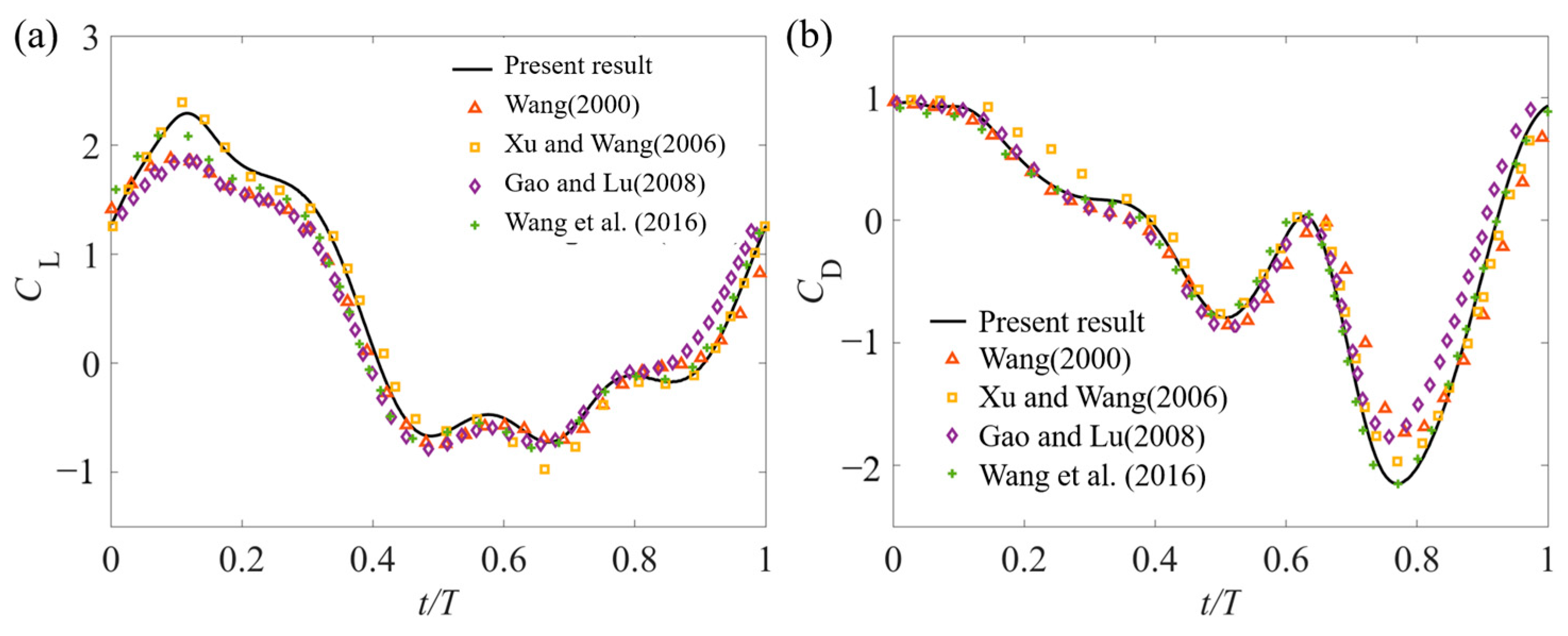
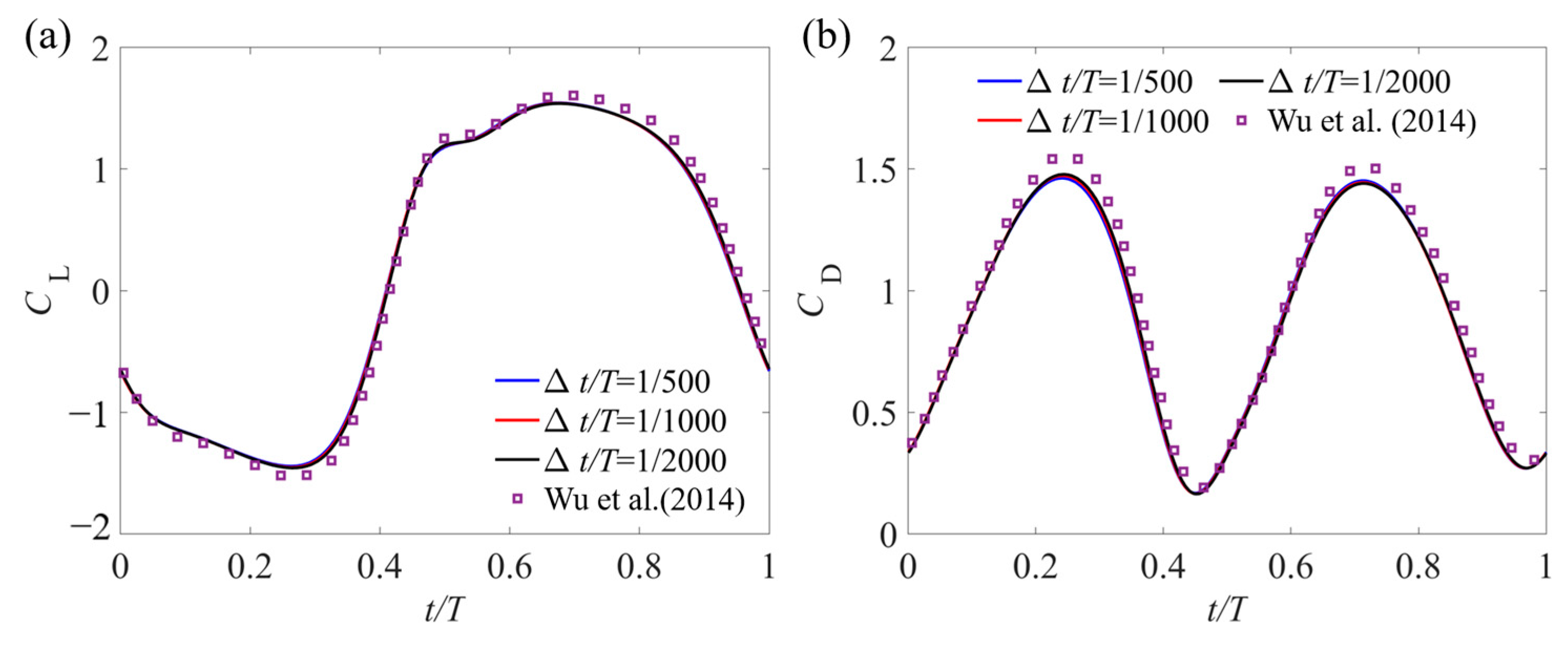
2.2. Validations of the Numerical Method

To validate the adopted numerical method, a comparison with the results reported by Wang [40] is carried out. Figure 3 shows the temporal evolution of the drag coefficient (C_D) and that of the lift coefficient (C_L). It is shown that the present results agree well with those of Wang. Moreover, to ensure the grid independence study, three grid sizes are tested: coarse (background grid: 130,000, component grid: 7000), middle (background grid: 270,000, component grid: 15,000), and fine (background grid: 540,000, component grid: 30,000). Taking the calculations of the fine grid as the benchmark, the averaged lift coefficient of the coarse grid differs by 3.80%, and the averaged thrust coefficient differs by 1.06%. For the middle grid, the averaged lift coefficient differs by 0.37%, and the averaged thrust coefficient differs by 0.09%. As also shown in Figure 4a,b, there is little difference between the middle-sized grid and the fine-sized grid, so the middle-sized grid is selected for the present study. For the time step independence, Figure 5a,b show that the results for Δt/T = 1/1000 and Δt/T = 1/2000 are close, but Δt/T = 1/500 shows significant discrepancies. Quantitatively, if the result of Δt/T = 1/2000 is taken as the reference, the time-averaged lift and drag at Δt/T = 1/500 differ by 2.28% and −0.19%, respectively, while at Δt/T = 1/1000, the time-averaged lift and drag differ by only 0.68% and −0.08%, respectively. Therefore, Δt/T = 1/1000 is employed, which offers a good compromise between the accuracy and resources. In addition, Figure 4 and Figure 5 show that the current results are in good agreement with those of Wu et al. [22].

2.3. Neural Network Modeling of the Unsteady Aerodynamic Parameters

Numerical simulations of high-precision unsteady aerodynamic characteristics for flapping wings necessitate significant computational power, since one always needs to numerically solve the nonlinear Navier–Stokes equations. Therefore, it is imperative to develop a neural network model that can predict the aerodynamic characteristics of arbitrary design parameters within the parameter space.

Time-series neural networks are abstract models capable of handling complex sequence data, simulating the operation of human brain neurons through numerous node connections and computations [43]. One such model is the gated recurrent unit (GRU) proposed by Cho et al. [34], which introduces a gating mechanism, including an update gate and a reset gate, as shown in Figure 6a. Traditional GRUs only process forward information in time series. To further exploit the feature information of time-series aerodynamic performance data, this paper adopts the bidirectional gate recurrent unit (BiGRU), which processes data in both the forward and backward directions. The network structure is shown in Figure 6b.

This work constructs a time series neural network with BiGRU at its core. The time-series neural network consists of 1 input layer, 2 BiGRU layers, 4 fully connected layers, and 1 output layer. The 2 BiGRU layers contain 256 and 128 hidden units, and the fully connected layer contains 128, 128, 64, and 64 hidden units.

Following the aforementioned neural network structure, a neural network surrogate model is developed based on the PyTorch framework to predict the near-ground tandem wing aerodynamic performance. The ground distance h/c and the phase difference φ between the front and rear wings are selected as the input parameters, which are consistent with the range of parameters in our numerical simulations. The range of h/c values is 0.875 ≤ h/c ≤ 5, and the range of φ values is −180 ≤ φ ≤ 180. There are 84 combinations of h/c and φ values, and each set of input parameters corresponds to C_L,mean, C_T,mean, and C_P,mean of the front wing and the rear wing, which are both time-equidistant sequences of length 1000 × 1, representing a periodic flapping cycle. Therefore, there are a total of 84 samples, with 10% of the samples selected as the test set and the remaining samples used as the training set. For the optimizer, the Adam optimizer [44] is used. The activation function uses Leaky ReLU, and the calculation formula is as follows:

$$\mathrm{LeakyReLU}(x)=\left\{\begin{array}{cc}x& x>0\\ \alpha x& x\le 0\end{array}\right.,$$

(7)

where a represents the negative slope and the empirical parameter is 1/5.5 [45].

The loss function adopts a Mean Squared Error (MSE) loss function with a weight correction. Due to the drastic changes in aerodynamic performance indicators near the ground, some aerodynamic performance indicators even show an exponential trend when close to the ground. Therefore, it is necessary to set the weights of samples at different ground distances h/c during model training. When 1.5 < h/c ≤ 5, the sample weight is set to 1; when 1.25 < h/c ≤ 1.5, the sample weight is set to 1.5; when 1 < h/c ≤ 1.25, the sample weight is set to 2; when 0.875 < h/c ≤ 1, the sample weight is set to 4; when h/c = 0.875, the sample weight is set to 5. This weight distribution method can improve the prediction accuracy of the model under conditions close to the ground. The difference in weight coefficients directly affects the calculation process of the mean square loss error function of the neural network model. The definition of MSE of the time series neural network with a weight correction is as follows:

$$MSE={\displaystyle \frac{1}{nT}}{\displaystyle \sum _{i=1}^n{\displaystyle \sum _{t=1}^T{w}_i{(y_{it}-{\widehat{y}}_{it})}^2}},$$

(8)

where n is the number of samples, T is the length of the time series, $w_i$ is the weight coefficient of the i-th sample, $y_{it}$ is the CFD result of the i-th sample at the t-th time step, and ${\widehat{y}}_{it}$ is the predicted value of the i-th sample at the t-th time step.

The complete neural network training process is summarized as follows:

• Obtaining the input data. The original data are obtained by the verified numerical simulations, and the data are preprocessed to obtain the training set and the test set.
• Forward propagation. The input data are used to predict the aerodynamic coefficient or energy consumption coefficient predicted by the neural network under the current parameters.
• Calculating the loss. The mean square error loss between the current predicted values of the aerodynamic coefficient and energy consumption coefficient and the CFD results is calculated.
• Backward propagation and update of the model parameters. Backward propagation is performed, the gradient is calculated through the defined Adam optimizer, and the parameters of the neural network model are updated.
• The above steps are repeated until the mean square error loss is small enough.

After iterations, the final MSE of different training objectives in this study is presented in

Table 1. The MSE of neural network training.

Target	The Initial MSE	Iterations	Learning Rate *	The Final MSE
$C_{\mathrm{L},\mathrm{fore}}$	3.32	30,000	0.01, 0.001, 0.0001	$4.21\times {10}^{-6}$
$C_{\mathrm{T},\mathrm{fore}}$	0.567	30,000	0.01, 0.001, 0.0001	$7.00\times {10}^{-7}$
$C_{\mathrm{P},\mathrm{fore}}$	1.93	30,000	0.01, 0.001, 0.0001	$1.90\times {10}^{-6}$
$C_{\mathrm{L},\mathrm{hind}}$	3.92	30,000	0.01, 0.001, 0.0001	$1.07\times {10}^{-5}$
$C_{\mathrm{T},\mathrm{hind}}$	0.681	30,000	0.01, 0.001, 0.0001	$1.69\times {10}^{-6}$
$C_{\mathrm{P},\mathrm{hind}}$	2.05	30,000	0.01, 0.001, 0.0001	$3.47\times {10}^{-6}$

* The learning rate of 0.01 is adopted in the initial stage of training. The larger learning rate makes the model converge quickly, and the learning rate decreases to 0.001 in 2000 iterations and 0.0001 in 9000 iterations. The smaller learning rate can improve the stability and precision of training.

, and it is reduced to about $1\times {10}^{-5}$, ensuring that the current model training has a good convergence degree, and the predicted results of the current neural network model parameters can match the CFD results well.

3. Results and Discussion

In this section, we present and discuss the results of tandem wings with different phase differences between the front and rear wings. In the following discussions, the influence of the ground effect and that of the phase difference are considered separately. The simulations are performed with the following parameters: the ground clearance h = 0.875 c, 1 c, 1.25 c, 1.5 c, 2 c, 3 c, 4 c, 5 c, and ∞ (free-flight case) and phase differences φ = −135°, −90°, −45°, 0°, 45°, 90°, 135°, and 180°. We first discuss the ground effect on aerodynamic parameters, and then the vortex structure of the flow is discussed in detail. In the end, a data-driven surrogate model is developed to predict the unsteady aerodynamic characteristics of tandem flapping wings under the ground effect.

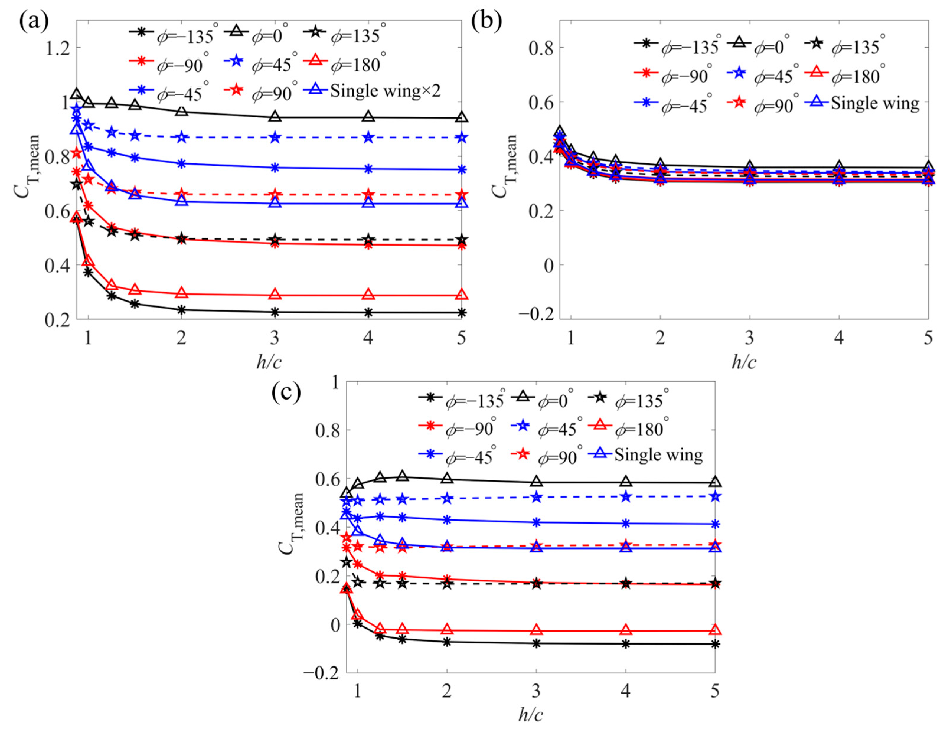
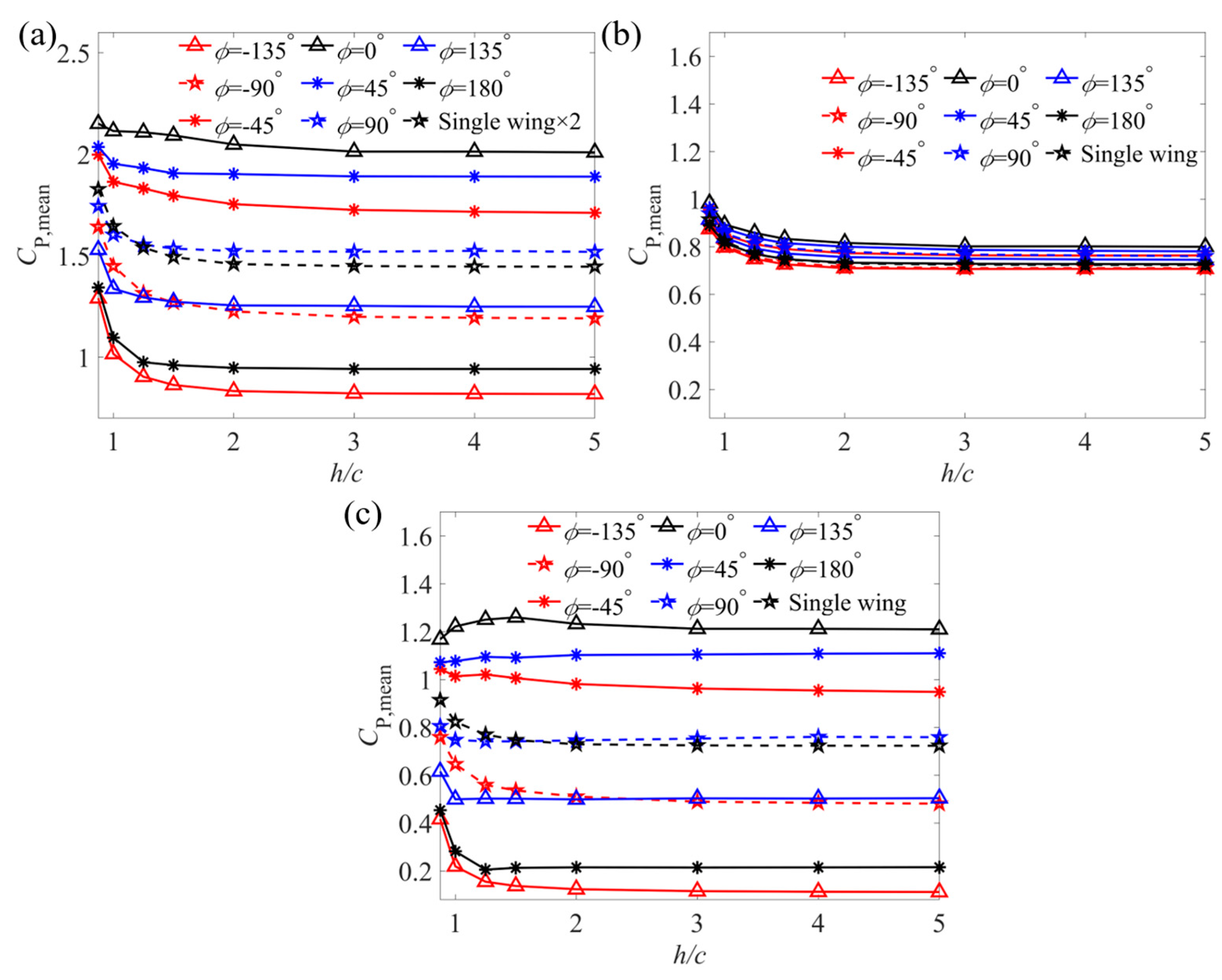
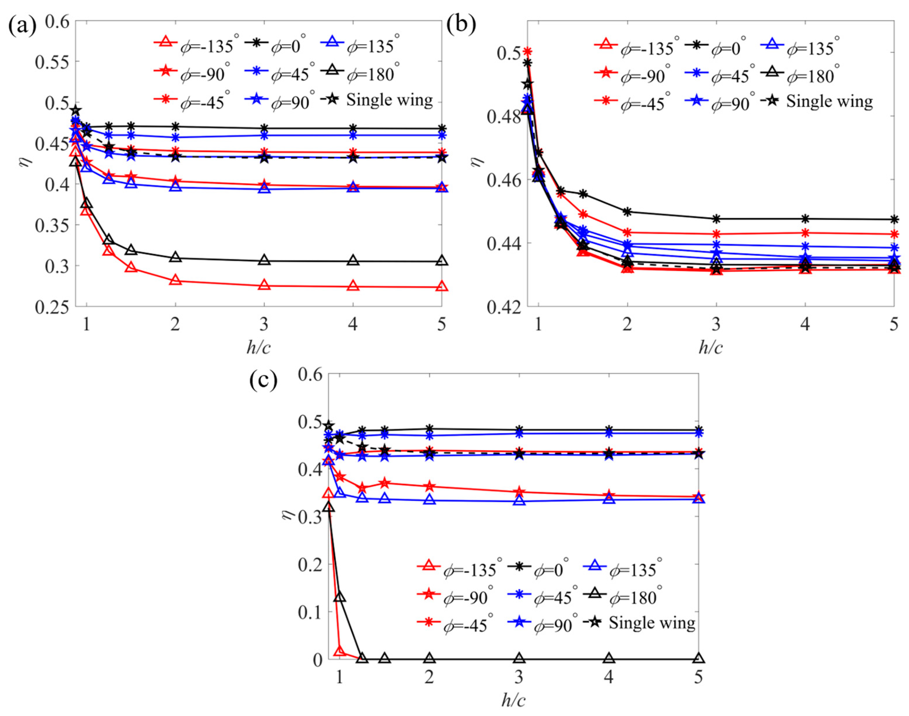
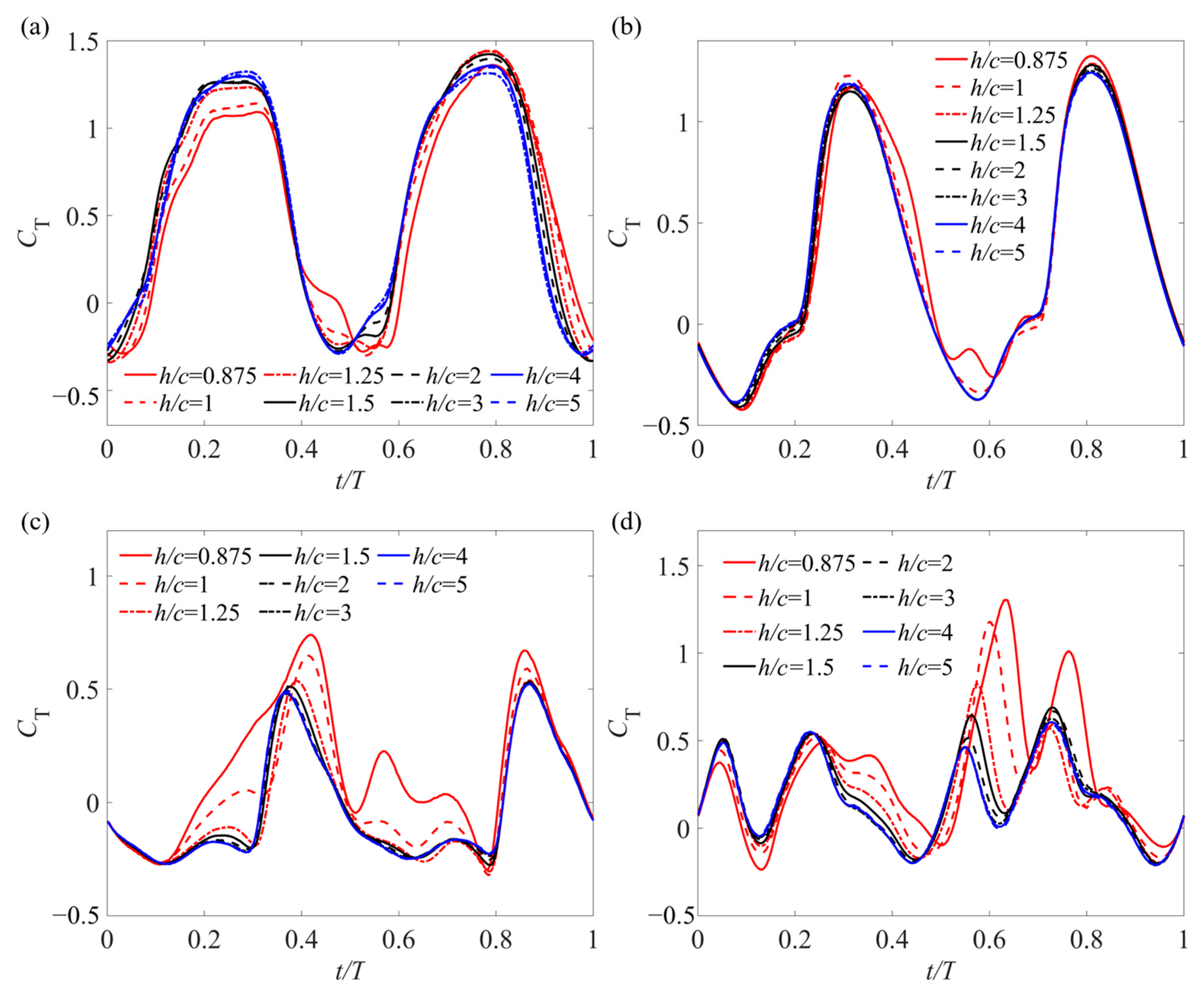
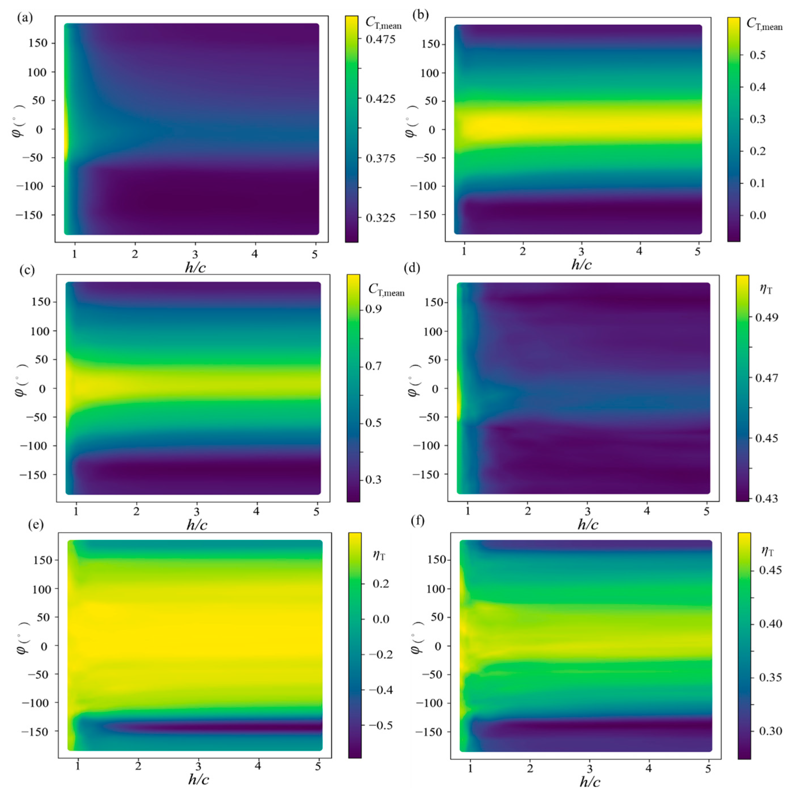
3.1. Effect of the Ground on the Aerodynamic Parameters

For tandem wings near the ground, as shown in Figure 7a, the total thrust coefficient, C_T,mean, increases monotonically with decreasing ground clearance, and this trend becomes significant when h/c < 3. Moreover, near the ground, the C_T,mean of tandem wings exhibits different increasing patterns under different phase differences, which can be explained by how the ground affects the propulsive performance of each wing individually.

As shown in Figure 7b,c, the C_T,mean of the tandem wings is decomposed into its front and rear wing components. The curves of C_T,mean of the front wing versus h/c are similar under different phase differences. They all increase with decreasing h/c and almost coincide with each other. This suggests that the ground effect on the front wing thrust enhancement is not sensitive to the phase difference. This is largely attributed to the fact that, in the forward flight, the front wing is located upstream of the incoming flow, while the rear wing is located downstream. The vortex structures induced by the hindwing have little influence on the vortex structure around the front wing.

For the rear wing, C_T,mean varies with h/c depending on the phase difference, φ. When φ = 0° or 45°, C_T,mean decreases as h/c decreases; when φ = −45° or 90°, C_T,mean increases as h/c decreases, but the increase is smaller than that of a single wing due to the ground effect; when φ = −135°, −90°, 135° or 180°, C_T,mean increases as h/c decreases, and the increase is larger than that of a single wing due to the ground effect. It is demonstrated that there is a coupling effect between the ground clearance and phase difference, and the phase difference plays a dominant role, comparatively speaking. In other words, there is a coupling relationship between the ground effect and the wing–wake interaction, which is not a simple superposition of the two acting separately.

As shown in Figure 8, for the C_P,mean of the tandem wing, front wing, and rear wing, the variation trend with h/c is similar to that of C_T,mean. As the thrust changes, the energy consumption also undergoes similar changes.

As shown in Figure 9, for the propulsion efficiency, η, the effect of the phase difference on η is much greater than that of h/c. For the front wing, the curves of η versus h/c are similar for different phase differences, and they all increase as the h/c decreases. However, the propulsion efficiency, η, of the front wing is often slightly greater than that of a single wing, which indicates that the rear wing has a negligible enhancement effect on η of the front wing. The difference in η of the tandem wings still depends mainly on the rear wing. However, the rear wing shows mixed results for different phase differences. When $\left|\varphi \right|$ is small (the rear wing slightly leads or lags behind the front wing), η is often higher, and can even reach 0.48 under in-phase flapping. However, as h/c decreases, the increase in η under the ground effect is also small, and even leads to a decrease under in-phase flapping. This indicates that when the rear wing leads or lags slightly, as it approaches the ground, the wing–wake interaction is not conducive to improving the propulsion efficiency of the rear wing compared to that of a single wing. When $\left|\varphi \right|$ is large (the rear wing is significantly ahead or lagging behind the front wing), the η of the rear wing is low, and sometimes, it cannot even produce a positive propulsion force. (In Figure 9c, the negative η is recorded as 0). However, when the wing is close to the ground, the ground effect will significantly improve its propulsion efficiency. This shows that, under the ground effect, the wing–wake interaction has a positive impact.

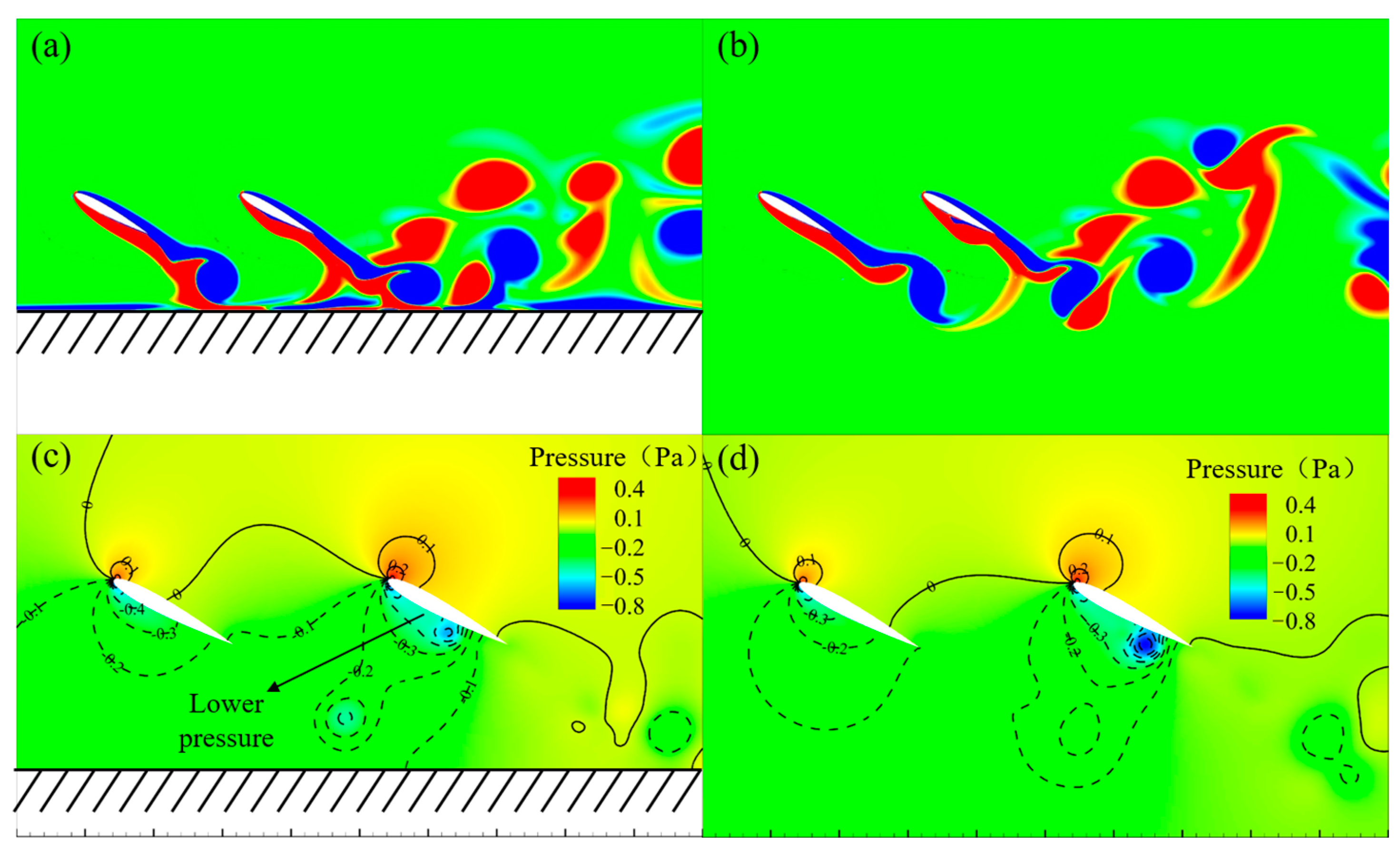
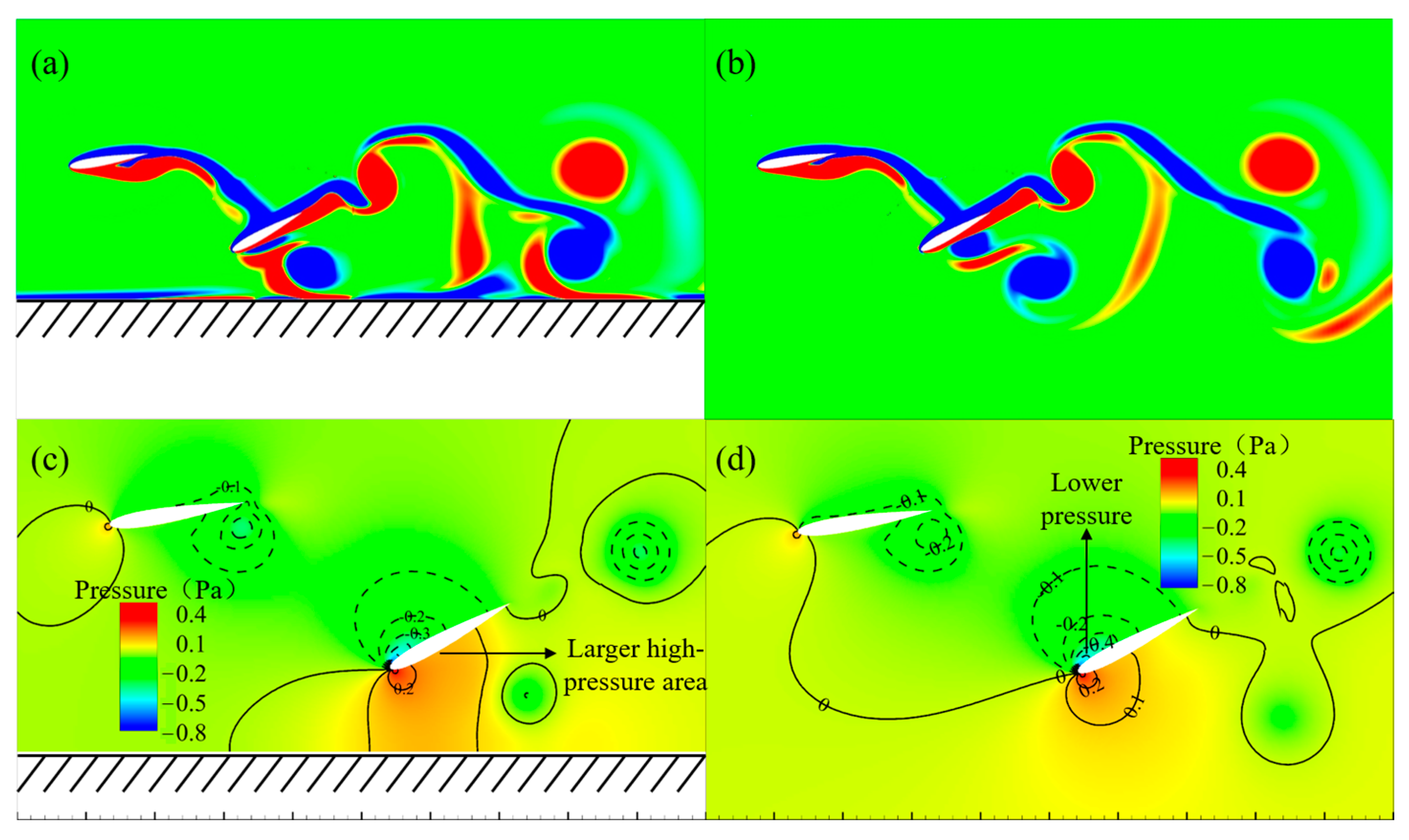
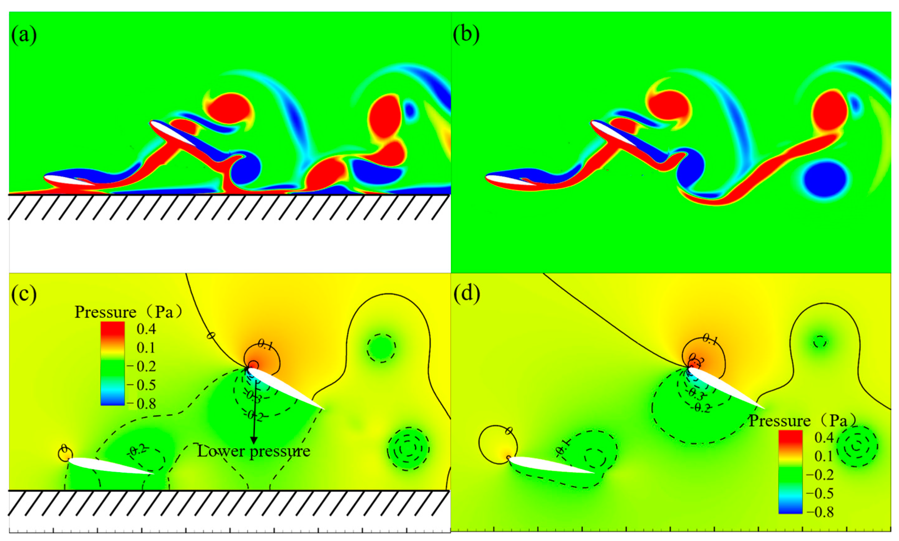
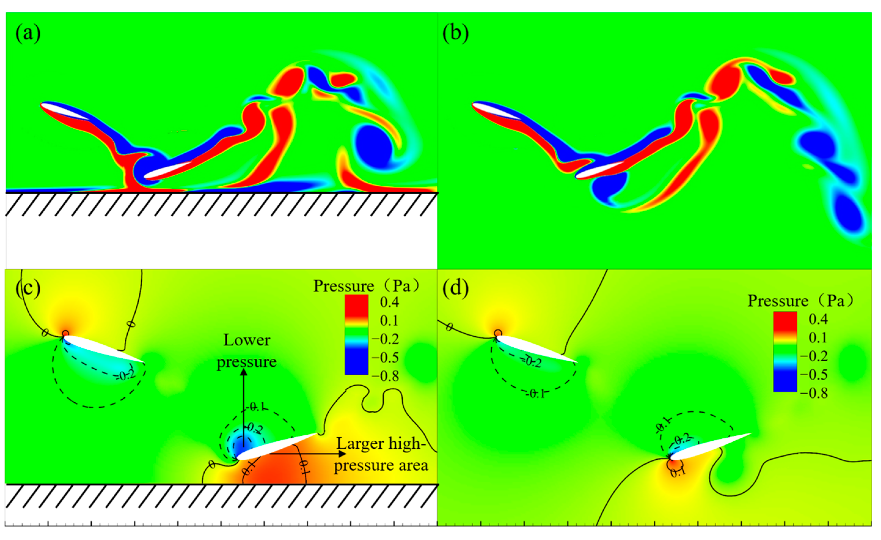
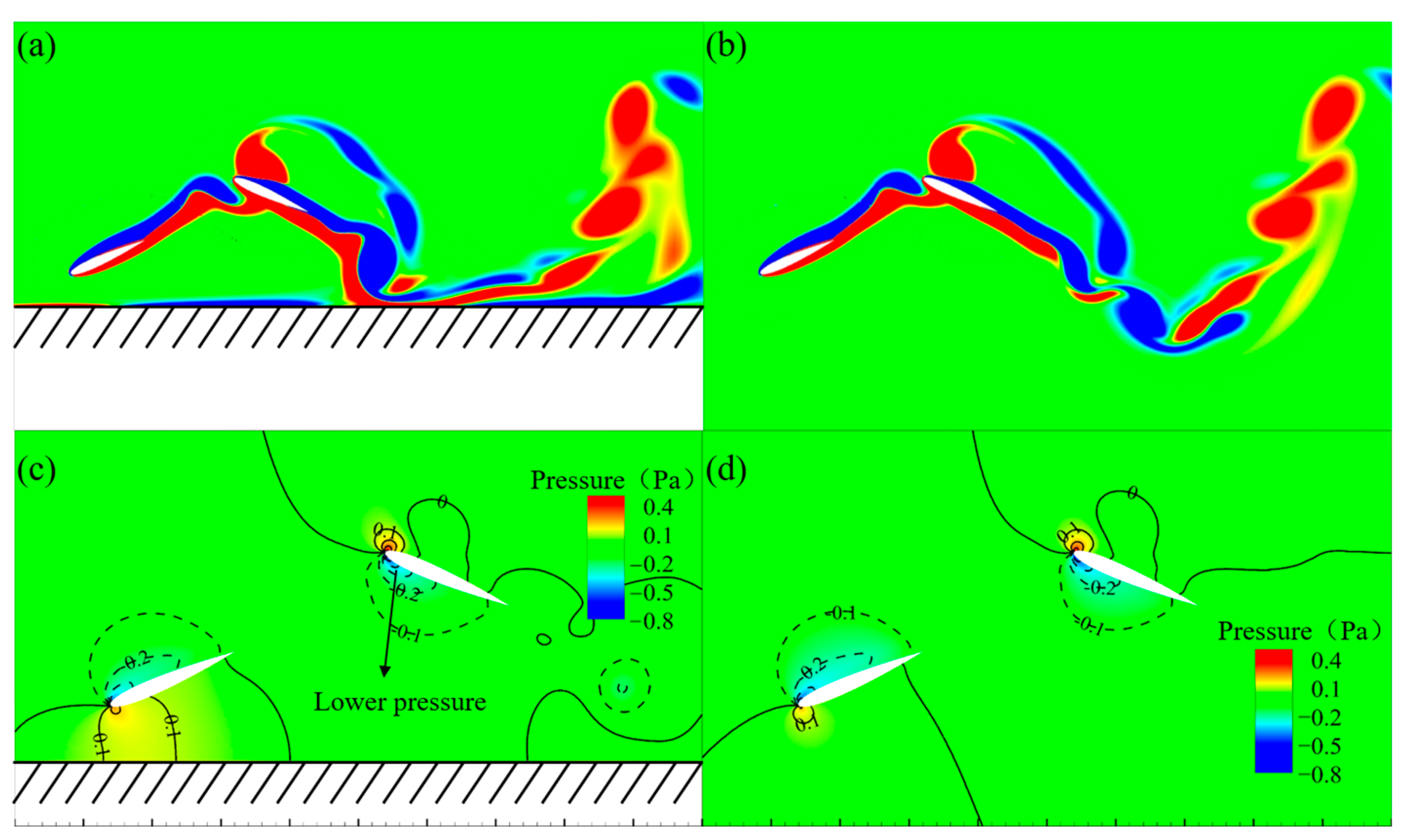
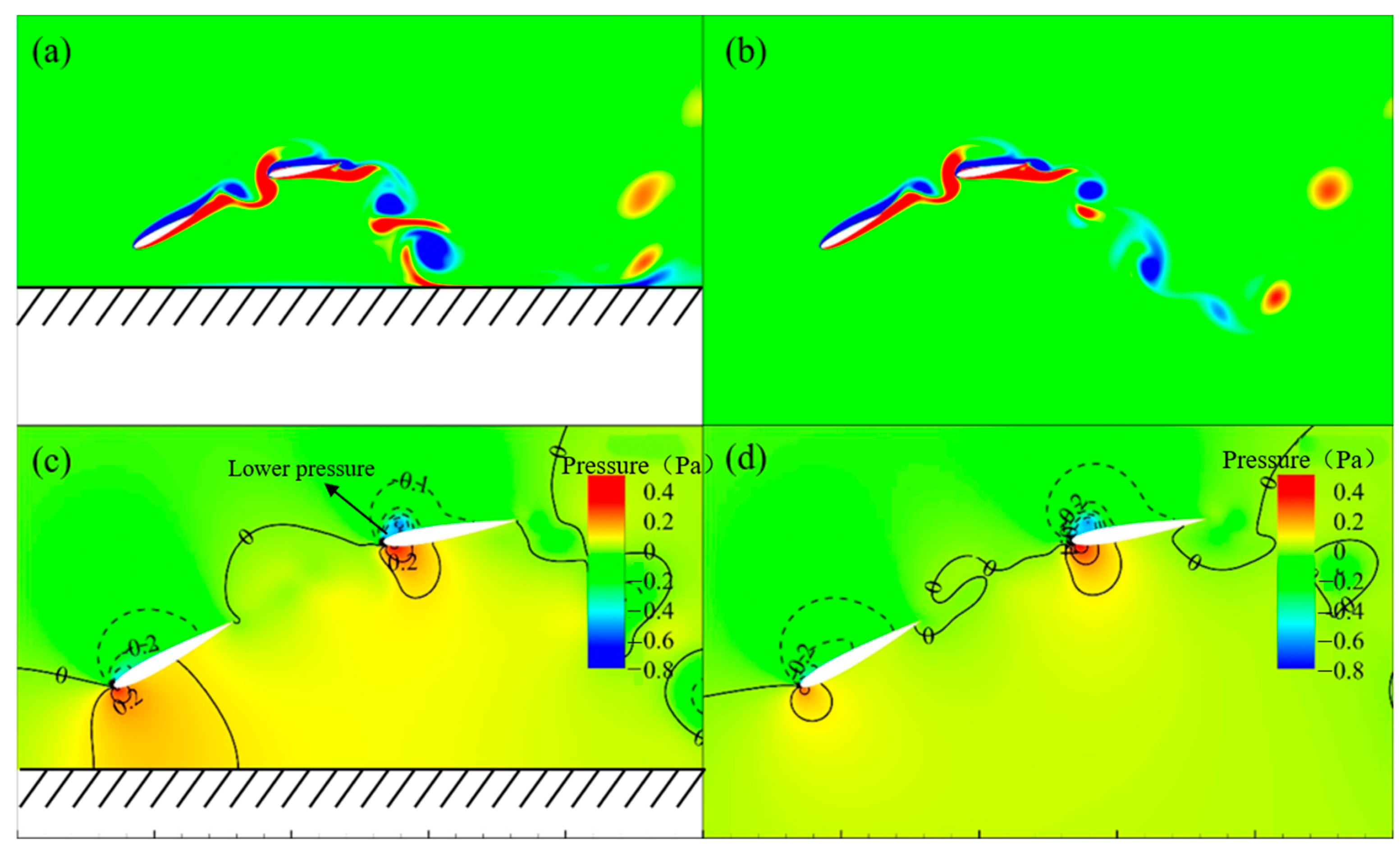
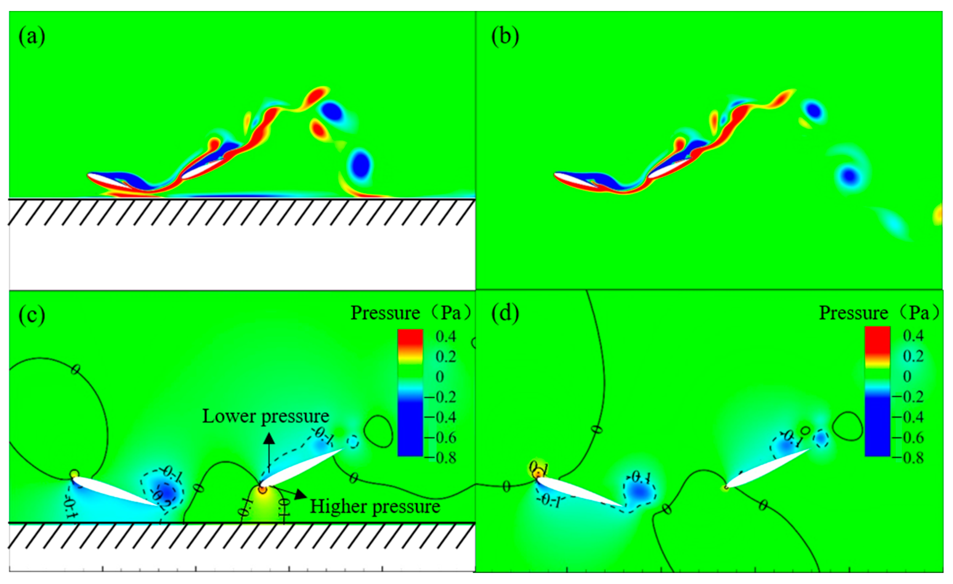
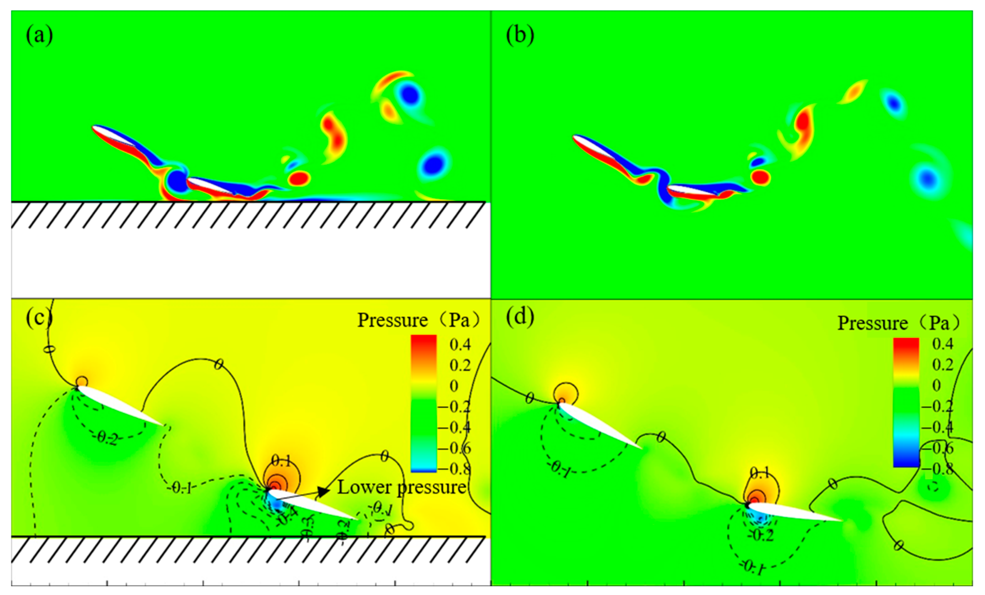
3.2. Effect of the Ground on Vortex Structure Evolution

The ground effect on the vortex structure and pressure distribution of tandem wings is also studied. It is the key to understanding the aerodynamic behaviors of the wings. Based on the previous analysis, according to the impact of the ground effect on the propulsion performance and its physical model, four typical conditions are selected:

• For φ = 0° (in-phase flapping), the smaller h/c is, the smaller C_T,mean is.
• For φ = 90° (the rear wing is ahead of the front wing), the smaller h/c is, the larger C_T,mean is, but the increase is less than that of the ground effect on a single wing.
• For φ = −90° (the rear wing lags behind the front wing), the smaller h/c is, the larger C_T,mean is, and the increase is greater than that of the ground effect on a single wing.
• For φ = 180° (anti-phase flapping), the smaller h/c is, the larger C_T,mean is, and the increase is greater than that of the ground effect on a single wing.

Figure 10 shows the instantaneous thrust coefficient C_T versus t/T in a steady flapping period under four phase differences. In four cases, C_T peaks occur at the same time as the interaction between the rear wing and the shedding wake. Therefore, for each typical condition, the occurrence time of C_T peaks in the upstroke and the downstroke, that is, the interaction time between the rear wing and the shedding wake, which is selected to analyze the influence of the ground effect on the vortex structure and pressure distribution around the rear wing.

When φ = 0° (in-phase flapping), in the downstroke, the closer to the ground, the lower the CT peak value. As shown in Figure 11, when t/T = 0.2, the rear wing passes through the CW (clockwise) wake, and the CW vortex on the upper surface is strengthened, while the CCW (counter clockwise) vortex on the lower surface is suppressed. However, while approaching the ground, due to the narrow space, a low-intensity high-pressure area is formed between the ground and the rear wing, which is slightly lower than that of the lower surface of the rear wing during the downstroke. The gap is small and does not have a significant impact on the pressure distribution on the lower surface. But it has a significant effect on the low-pressure zone on the upper surface, resulting in a reduction in the low-pressure zone. As a result, the pressure difference between the upper and lower surfaces of the wing is reduced and the C_T of the rear wing is reduced.

During the upstroke, as shown in Figure 10a, the closer to the ground, the higher the C_T peak value at h/c = 1–5. In Figure 12, when t/T = 0.8, the rear wing passes through the shaded CCW wake and the CW vortex on the upper surface is weakened, while the CCW vortex on the lower surface is strengthened. Considering the ground effect, the rear wing during the upstroke is gradually away from the ground, a low-pressure area is formed between the ground and the wing, and the low-pressure area on the lower surface of the rear wing strengthens and expands, which leads to the increase in the peak value of the instantaneous propulsion force.

When φ = 90°, during the downstroke, as shown in Figure 10b and Figure 13, the peak value of the instantaneous propulsion force will decrease at first (1.5 < h/c < 5) and then increase (0.875 < h/c < 1.5). In 1.5 < h/c < 5, the rear wing passes through the shedding wake, and the effect on the rear wing is similar to that when φ = 0°, resulting in a decrease in the C_T peak value. In 0.875 < h/c < 1.5, because the wing–wake interaction is later than that of φ = 0°, the position of the C_T peak moves closer to the end of the downstroke, which is more strongly affected by the ground effect. At this position, not only is the low-pressure area on the upper surface of the wing weakened, but also, the high-pressure area on the lower surface is strengthened, which increases the pressure difference between the upper and lower surface and leads to the increase in the C_T peak value at 0.875 < h/c < 1.5.

During the upstroke, as shown in Figure 12 and Figure 14, the occurrence time of the wing–wake interaction is close to that of φ = 0°. The mechanism of the ground effect is also similar, which leads to an increase in the C_T peak value of the rear wing.

When φ = 180° (anti-phase flapping), as shown in Figure 15, the position of the wing–wake interaction is close to the end of the downstroke. Compared with the cases with φ = 0° and φ = 90°, because of the wing–wake interaction, the high-pressure area on the lower surface of the wing is destroyed, the time of the peak propulsion force is delayed, and the peak value is also reduced. Therefore, the wing–wake interaction has a destructive effect on the propulsion force when in anti-phase flapping. When the wing–wake interaction occurs (t/T = 0.4), it is also closer to ground, and the ground effect is stronger than that of φ = 0° and φ = 90°. On one hand, the ground leads to a strong high-pressure area under the rear wing, which enhances the high-pressure area on the lower surface to a great extent. On the other hand, the ground hinders the dissipation of the CW wake, and the CW vortex on the upper surface of rear wing is continuously affected, which leads to a slight enhancement of the high-pressure area on the upper surface. The two factors couple and lead to an enhancement of the C_T peak value during the downstroke.

During the upstroke, as shown in Figure 16, the mechanism of the ground effect is also similar to the cases with φ = 0° and φ = 90°. However, when φ = 180°, the C_T peak appears at about t/T = 0.85, yet when φ = 0 °and 90°, it appears at about t/T = 0.8. Therefore, the rear wing is closer to the ground and is more strongly affected by the ground effect.

When φ = −90°, the composition of the vortex distribution is complicated, and the rear wing meets the wake of the front wing four times in a stable flapping period. As shown in Figure 15d, there are four C_T peaks, which are different from the two C_T peaks observed under other typical conditions.

Figure 17 and Figure 18 show the vorticity contours and pressure contours at the typical instants in the downstroke. The ground effect slightly reduces the first C_T peak. As shown in Figure 17, the rear wing passes through the CCW wake from the front wing. In the ground effect, the shedding wake intensity increases due to the narrow space, resulting in a weaker CW vortex of the opposite sign on the upper surface of the rear wing. The negative pressure along the upper surface is also lower, and the pressure difference and C_T peak are reduced.

The second C_T peak appears at t/T = 0.25, and the ground has little effect on it. However, the ground effect significantly improves C_T after the second peak during the downstroke. Therefore, t/T = 0.35 is taken as the second typical instant. When t/T = 0.35 and h/c = ∞, on one hand, the rear wing continuously coincides with the CCW wake from the front wing, which causes the LEV (leading edge vortex) of the rear wing to fall off ahead of time, and the high-pressure area at the leading edge of the lower surface decreases; on the other hand, because the CCW wake continues to interact with the CW vortex on the upper surface of the rear wing, the CW vortex decreases and C_T is relatively low. Considering the ground effect, at h/c = 1, due to the narrow space, the ground effect induces a high-pressure area under the rear wing, which significantly enhances the LEV of the rear wing. At the same time, the high-pressure zone causes the CCW wake of the front wing shift slightly upward, reducing the damage to the CW vortex on the upper surface. This leads to an enhancement of C_T. At t/T = 0.35, the mechanism is similar to that at t/T = 0.25–0.45.

In the upstroke, there are also two C_T peaks, as shown in Figure 10d. For the first C_T peak, the closer to the ground, the greater the C_T peak value and the later the C_T peak appears. As shown in Figure 19, two typical moments are taken: h/c = 1, t/T = 0.60 and h/c = 5, t/T = 0.55. At h/c = 1, t/T = 0.60, the CW wake from the front wing contacts the rear wing, which causes the LEV on the rear wing fall off ahead of time and results in an earlier C_T peak. Considering the ground effect, at h/c = 5 and t/T = 0.55, the ground hinders the downward dissipation of the CW wake, which strengthens the CW vortex of the same sign on the upper surface of the rear wing. At the same time, because the ground induces a strong low-pressure zone between the rear wing and the ground, the low-pressure zone on the lower surface of the rear wing is also enhanced, which significantly increases the pressure difference and the C_T peak.

As shown in Figure 20, for the second peak during the upstroke, the CCW vortex on the lower surface of the rear wing contracts the CW wake, resulting in the weakening of the CCW vortex. In the ground effect, the change in the C_T peak value is small, but the change is more complicated than that for the other C_T peaks. From h/c = 5 to h/c = 1.5, the mechanism of the ground effect is similar to that of a single wing during the upstroke. The rear wing flaps away from the ground, and the ground has a slight attraction to the wing, leading to an increase in the C_T peak. From h/c = 1.5 to h/c = 0.875, on the one hand, the closer ground blocks the wake, which prevents the wake from dissipating in time and aggravates the interference between the CW wake and the CCW vortex on the lower surface. This factor is not conducive to the generation of low-pressure regions. On the other hand, as h/c decreases, the low-pressure zone between the rear wing and the ground becomes stronger, which compensates for the low-pressure zone of the rear wing. This factor plays a conducive role. When the C_T peak decreases from h/c = 1.5 to h/c = 1.25, the former factor plays a dominant role. On the contrary, when the C_T peak increases from h/c = 1.25 to h/c = 0.875, the latter factor is dominant.

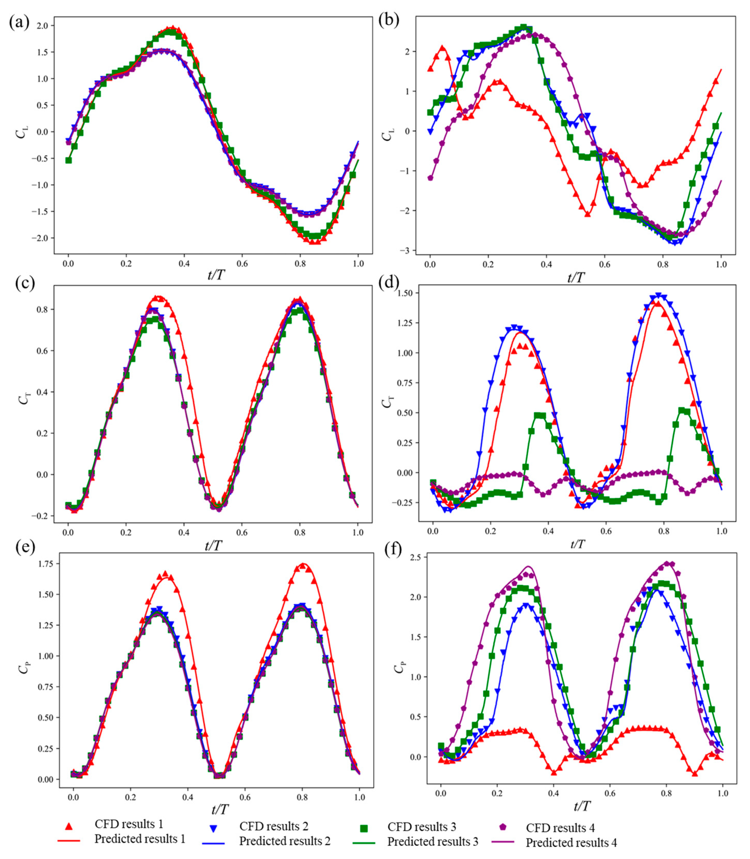
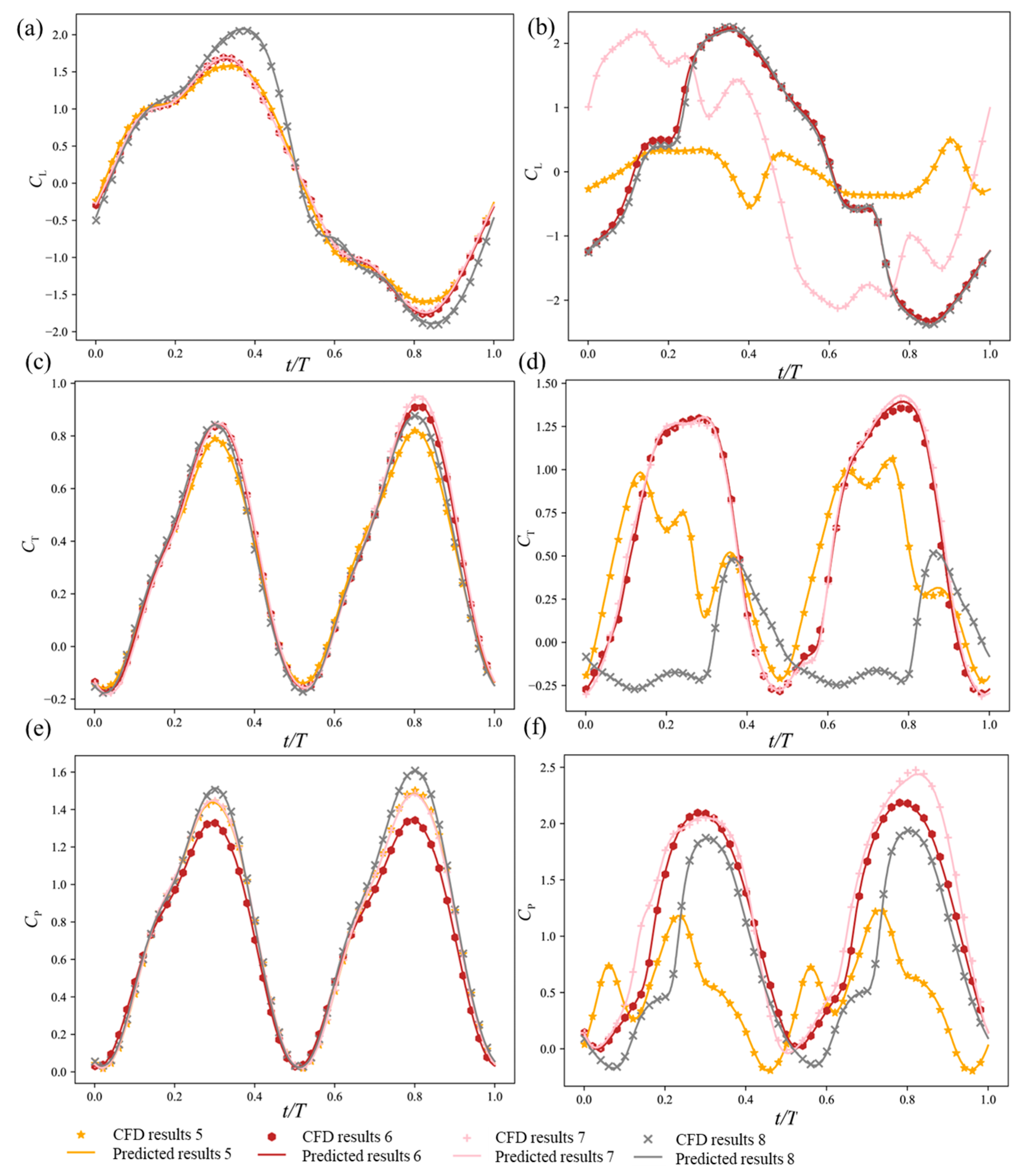
3.3. Aerodynamic Performance Prediction

In the evaluation of the aerodynamic performance, the time-averaged aerodynamic force coefficient within a flapping cycle is crucial. Table 1 introduces two error measurement indicators to assess the discrepancy between the neural network predictions on the test set and the CFD results.

The relative error $\delta$ can be used to measure the error results of the time-averaged coefficient and energy consumption coefficient, and it reads:

$$\delta ={\displaystyle \frac{\widehat{y}-y}{y}}\times 100\%,$$

(9)

where $\widehat{y}$ is the predicted result of the time-averaged force coefficient and $y$ is the CFD result of the time-averaged force coefficient. However, the relative error becomes an insufficient metric when the time-averaged lift coefficient approaches zero during flapping far from the ground. In such cases, the root mean square error (RMSE) is a more suitable measure. The RMSE is utilized to assess the error in the instantaneous force coefficient and instantaneous energy consumption coefficient. The formula for the RMSE is:

$$RMSE=\sqrt{{\displaystyle \frac{1}{n}}{\displaystyle \sum _{i=1}^n{\left(y_i-\widehat{y_i}\right)}^2}},$$

(10)

where n is the number of time series within a flapping cycle (n = 1000), $y_i$ is the CFD result of the ith time series data within a flapping cycle, and $\widehat{y_i}$ is the predicted result of the ith time series data.

Figure 21 and Figure 22 illustrate the discrepancies between the predicted and CFD results for various coefficients of the front and rear wings on the test set. The figures demonstrate a high degree of consistency between the predictions and CFD results, validating the accuracy of the trained neural network. However, due to significant variations in the force and energy consumption coefficients of the rear wing near the ground, the neural network exhibits some deviations in regions with larger gradient changes (0.875 ≤ h/c ≤ 1), despite the correction of loss function weights for samples at different ground distances.

Table 2. Error of the neural network on the test set.

Training Objective	Percentage of Test Sets Total Samples	Average Relative Error	Relative Error with the Maximum Absolute Value	Average RMSE	Maximum RMSE
$C_{\mathrm{L},\mathrm{fore}}$	10%	—— *	—— *	0.01551	0.03021
$C_{\mathrm{L},\mathrm{hind}}$	10%	—— *	—— *	0.02330	0.05354
$C_{\mathrm{T},\mathrm{fore}}$	10%	0.3686%	1.442%	0.005820	0.01510
$C_{\mathrm{T},\mathrm{hind}}$	10%	1.165%	−3.506%	0.02265	0.09046
$C_{\mathrm{P},\mathrm{fore}}$	10%	0.2518%	−0.6413%	0.009269	0.02499
$C_{\mathrm{P},\mathrm{hind}}$	10%	0.7245%	−2.597%	0.02912	0.09981

* The relative error is an insufficient metric when the time-averaged lift coefficient approaches zero during flapping far from ground. In such cases, the root mean square error (RMSE) is a more suitable measure.

presents the time-averaged values, demonstrating minimal error. The relative error with max value among all samples is −3.5%, which can be attributed to the limited sample size and incomplete learning of time series features by the neural network. Nevertheless, the overall error is sufficiently small, indicating the high accuracy of the established neural network model in predicting aerodynamic performance. Figure 23 illustrates the predicted aerodynamic performance of the tandem wings across the entire parameter space using this neural network.

As a summary, the time series neural network model effectively substitutes CFD calculations, accurately capturing the variations in the aerodynamic force coefficient and energy consumption coefficient under different parameter combinations within the flapping cycle. It serves as a highly accurate surrogate model for the transient aerodynamic performance of near-ground tandem flapping wings.

4. Conclusions

In this study, we discuss the effect of the ground on the aerodynamic performance of two wings in the tandem configuration in the forward flight mode in a numerical way. It is found that the wing–wake interaction and ground influence the propulsion characteristics of the rear wing in a coupled way. Different phase differences change the meeting time of the wake and the rear wing, thus leading to different ground effects on the propulsion performance of the rear wing. When the phase difference $\left|\varphi \right|$ is small (φ = −45°, 0°, 45°, and 90°), the thrust is generally high, and the boosting effect of the ground on the rear wing, which rises by 12.33% at maximum, is smaller than that on the single wing, which increases by 43.83%. One even observes a reduced thrust at the low phase difference of 0° and 45°. When $\left|\varphi \right|$ is large (φ = −135°, −90°, 135° and 180°), the thrust is usually low, and the boosting effect of the ground on the rear wing is greater than that of the ground effect on the single wing; a maximum increase of 43.83% is achieved.

In addition, a BiGRU-based neural network is employed to develop a surrogate model in order to effectively predict the unsteady aerodynamic performance for tandem-wing flapping flight. On the test set, the relative errors of the time-averaged values range from −4% to 2%, while the RMSE of the transient values is less than 0.1. The developed model offers a continuous description of the flow fields and the aerodynamic behavior throughout the flapping cycle in the parameter space from a mathematical point of view, rather than offering only the values on the discrete points, thus resulting in a precise representation of unsteady aerodynamics. At the same time, although this study considers only one simple plunging and pitching motion, other flapping motions can be also dealt with well, which does not cause any difference in the framework of the numerical method or that of the developed data-driven strategy. That is to say that the techniques in the present study demonstrate strong generalization capabilities and are readily applicable to investigating the mechanisms of flapping-wing aerodynamic characteristics across various parameters, dimensions, and application scenarios. In the end, it is necessary to point out that the size of the dataset needed for the surrogate model’s training is relatively large. In future work, introducing physics-informed constrains could be an effective way to reduce the training cost.

References

1. Lian, Y.; Broering, T.; Hord, K.; Prater, R. The characterization of tandem and corrugated wings. Prog. Aerosp. Sci. 2014, 65, 41–69. [Google Scholar] [CrossRef]
2. Chin, D.D.; Lentink, D. Flapping wing aerodynamics: From insects to vertebrates. J. Exp. Biol. 2016, 219, 920–932. [Google Scholar] [CrossRef] [PubMed]
3. Haider, N.; Shahzad, A.; Mumtaz Qadri, M.N.; Ali Shah, S.I. Recent progress in flapping wings for micro aerial vehicle applications. Proc. Inst. Mech. Eng. Part C J. Mech. Eng. Sci. 2021, 235, 245–264. [Google Scholar] [CrossRef]
4. Han, J.-H.; Han, Y.-J.; Yang, H.-H.; Lee, S.-G.; Lee, E.-H. A Review of Flapping Mechanisms for Avian-Inspired Flapping-Wing Air Vehicles. Aerospace 2023, 10, 554. [Google Scholar] [CrossRef]
5. De Manabendra, M.; Sudhakar, Y.; Gadde, S.; Shanmugam, D.; Vengadesan, S. Bio-inspired Flapping Wing Aerodynamics: A Review. J. Indian Inst. Sci. 2024, 104, 181–203. [Google Scholar] [CrossRef]
6. Li, D.; Mu, Y.; Lau, G.-K.; Chin, Y.; Lu, Z. Numerical study on the aerodynamic performance of dragonfly (Anax parthenope julius) maneuvering flight during synchronized-stroking. Phys. Fluids 2024, 36, 091911. [Google Scholar] [CrossRef]
7. Bomphrey, R.J.; Nakata, T.; Henningsson, P.; Lin, H.T. Flight of the dragonflies and damselflies. Philos. Trans. R. Soc. Lond. B Biol. Sci. 2016, 371, 20150389. [Google Scholar] [CrossRef]
8. Salami, E.; Montazer, E.; Ward, T.A.; Nik Ghazali, N.N.; Anjum Badruddin, I. Aerodynamic Performance of a Dragonfly-Inspired Tandem Wing System for a Biomimetic Micro Air Vehicle. Front. Bioeng. Biotechnol. 2022, 10, 787220. [Google Scholar] [CrossRef]
9. Pinapatruni, G.V.R.; Duddupudi, M.B.; Dash, S.M.; Routray, A. On the investigation of the aerodynamics performance and associated flow physics of the optimized tubercle airfoil. Phys. Fluids 2024, 36, 051907. [Google Scholar] [CrossRef]
10. Sinha, J.; Dash, S.M.; Lua, K.B. On the study of the pitch angular offset effects at various flapping frequencies for a two-dimensional asymmetric flapping airfoil in forward flight. Phys. Fluids 2024, 36, 041913. [Google Scholar] [CrossRef]
11. Gao, T.; Lu, X.Y. Insect normal hovering flight in ground effect. Phys. Fluids 2008, 20, 087101. [Google Scholar] [CrossRef]
12. Lu, H.; Lua, K.B.; Lim, T.T.; Yeo, K.S. Ground effect on the aerodynamics of a two-dimensional oscillating airfoil. Exp. Fluids 2014, 55, 1–15. [Google Scholar] [CrossRef]
13. Maeda, M.; Liu, H. Ground Effect in Fruit Fly Hovering: A Three-Dimensional Computational Study. J. Biomech. Sci. Eng. 2013, 8, 344–355. [Google Scholar] [CrossRef]
14. Umar, F.; Sun, M. Aerodynamic Force and Power for Flapping Wing at Low Reynolds Number in Ground Effect. In Proceedings of the International Bhurban Conference on Applied Sciences & Technology, Islamabad, Pakistan, 9–13 January 2018; pp. 553–558. [Google Scholar]
15. Zheng, Y.; Qu, Q.; Liu, P.; Hu, T. Ground Effect of a Two-Dimensional Flapping Wing Hovering in Inclined Stroke Plane. J. Fluids Eng. 2022, 144, 111206. [Google Scholar] [CrossRef]
16. Meng, X.; Zhang, Y.; Chen, G. Ceiling effects on the aerodynamics of a flapping wing with advance ratio. Phys. Fluids 2020, 32, 021904. [Google Scholar] [CrossRef]
17. Meng, X.; Ghaffar, A.; Zhang, Y.; Deng, C. Very low Reynolds number causes a monotonic force enhancement trend for a three-dimensional hovering wing in ground effect. Bioinspir. Biomim. 2021, 16, 055006. [Google Scholar] [CrossRef]
18. Meng, X.; Han, Y.; Chen, Z.; Ghaffar, A.; Chen, G. Aerodynamic Effects of Ceiling and Ground Vicinity on Flapping Wings. Appl. Sci. 2022, 12, 4012. [Google Scholar] [CrossRef]
19. Wang, L.; Yeung, R.W. Investigation of full and partial ground effects on a flapping foil hovering above a finite-sized platform. Phys. Fluids 2016, 28, 071902. [Google Scholar] [CrossRef]
20. Yin, B.; Yang, G.; Prapamonthon, P. Finite obstacle effect on the aerodynamic performance of a hovering wing. Phys. Fluids 2019, 31, 101902. [Google Scholar] [CrossRef]
21. Wu, J.; Zhao, N. Ground Effect on Flapping Wing. Procedia Eng. 2013, 67, 295–302. [Google Scholar] [CrossRef]
22. Wu, J.; Shu, C.; Zhao, N.; Yan, W. Fluid Dynamics of Flapping Insect Wing in Ground Effect. J. Bionic Eng. 2014, 11, 52–60. [Google Scholar] [CrossRef]
23. Mivehchi, A.; Dahl, J.; Licht, S. Heaving and pitching oscillating foil propulsion in ground effect. J. Fluids Struct. 2016, 63, 174–187. [Google Scholar] [CrossRef]
24. Lin, X.; Guo, S.; Wu, J.; Nan, J. Aerodynamic Performance of a Flapping Foil with Asymmetric Heaving Motion near a Wall. J. Bionic Eng. 2018, 15, 636–646. [Google Scholar] [CrossRef]
25. Li, Y.; Pan, Z.; Zhang, N. Numerical analysis on the propulsive performance of oscillating wing in ground effect. Appl. Ocean Res. 2021, 114, 1–16. [Google Scholar] [CrossRef]
26. Lin, C.; Jia, P.; Wang, C.; Zhong, Z. Fluid dynamics of a flapping wing interacting with the boundary layer at a flat wall. Phys. Fluids 2024, 36, 041917. [Google Scholar] [CrossRef]
27. Sun, M.; Lan, S.L. A computational study of the aerodynamic forces and power requirements of dragonfly (Aeschna juncea) hovering. J. Exp. Biol. 2004, 207, 1887–1901. [Google Scholar] [CrossRef]
28. Wang, Z.J.; Russell, D. Effect of Forewing and Hindwing Interactions on Aerodynamic Forces and Power in Hovering Dragonfly Flight. Phys. Rev. Lett. 2007, 99, 148101. [Google Scholar] [CrossRef]
29. Zhang, J.; Lu, X.-Y. Aerodynamic performance due to forewing and hindwing interaction in gliding dragonfly flight. Phys. Rev. E 2009, 80, 017302. [Google Scholar] [CrossRef]
30. Lua, K.B.; Lu, H.; Zhang, X.H.; Lim, T.T.; Yeo, K.S. Aerodynamics of two-dimensional flapping wings in tandem configuration. Phys. Fluids 2016, 28, 121901. [Google Scholar] [CrossRef]
31. Zheng, Y.; Wu, Y.; Tang, H. An experimental study on the forewing–hindwing interactions in hovering and forward flights. Int. J. Heat Fluid Flow 2016, 59, 62–73. [Google Scholar] [CrossRef]
32. Nagai, H.; Fujita, K.; Murozono, M. Experimental Study on Forewing-Hindwing Phasing in Hovering and Forward Flapping Flight. AIAA J. 2019, 57, 3779–3790. [Google Scholar] [CrossRef]
33. Sarbandi, A.; Naderi, A.; Parhizkar, H. The ground effect on flapping Bio and NACA 0015 airfoils in power extraction and propulsion regimes. J. Braz. Soc. Mech. Sci. Eng. 2020, 42, 287. [Google Scholar] [CrossRef]
34. Cho, K.; Van Merrienboer, B.; Gulcehre, C.; Bahdanau, D.; Bougares, F.; Schwenk, H.; Bengio, Y. Learning Phrase Representations Using RNN Encoder-Decoder for Statistical Machine Translation. In Proceedings of the EMNLP, Association for Computational Linguistics, Doha, Qatar, 25–29 October 2014. [Google Scholar]
35. Taylor, G.K.; Nudds, R.L.; Thomas, A.L.R. Flying and swimming animals cruise at a Strouhal number tuned for high power efficiency. Nature 2003, 425, 707–711. [Google Scholar] [CrossRef]
36. Younsi, A.; zamree bin abd Rahim, S.; Rezoug, T. Aerodynamic investigation of an airfoil under two hovering modes considering ground effect. J. Fluids Struct. 2019, 91, 102759. [Google Scholar] [CrossRef]
37. Rezaei, A.S.; Taha, H. Circulation dynamics of small-amplitude pitching airfoil undergoing laminar-to-turbulent transition. J. Fluids Struct. 2021, 100, 103177. [Google Scholar] [CrossRef]
38. Nawafleh, A.; Xing, T.; Durgesh, V.; Padilla, R. Fluid–structure interaction simulation of a flapping flag in a laminar jet. J. Fluids Struct. 2023, 119, 103869. [Google Scholar] [CrossRef]
39. Mozafari, M.; Sadeghimalekabadi, M.; Fardi, A.; Bruecker, C.; Masdari, M. Aeroacoustic investigation of a ducted wind turbine employing bio-inspired airfoil profiles. Phys. Fluids 2024, 36, 041918. [Google Scholar] [CrossRef]
40. Wang, Z.J. Two Dimensional Mechanism for Insect Hovering. Phys. Rev. Lett. 2000, 85, 2216–2219. [Google Scholar] [CrossRef]
41. Xu, S.; Wang, Z.J. An immersed interface method for simulating the interaction of a fluid with moving boundaries. J. Comput. Phys. 2006, 216, 454–493. [Google Scholar] [CrossRef]
42. Wang, C.; Zhou, C.; Xie, P. Numerical investigation on aerodynamic performance of a 2-D inclined hovering wing in asymmetric strokes. J. Mech. Sci. Technol. 2016, 30, 199–210. [Google Scholar] [CrossRef]
43. Liu, Z.; Zhu, Z.; Gao, J.; Xu, C. Forecast Methods for Time Series Data: A Survey. IEEE Access 2021, 9, 91896–91912. [Google Scholar] [CrossRef]
44. Kingma, D.P.; Ba, J. Adam: A Method for Stochastic Optimization. CoRR arXiv 2014, arXiv:1412.6980. [Google Scholar]
45. Xu, B.; Wang, N.; Chen, T.; Li, M. Empirical Evaluation of Rectified Activations in Convolutional Network. CoRR arXiv 2015, arXiv:1505.00853. [Google Scholar]
Figure 1. (a) Scheme of the tandem wing in forward flight mode. U0 is the velocity of horizontal fluid flow, L represents the distance between the front and rear wings, h represents the ground clearance, and A is the amplitude of the heave motion. The pivot point is on the central line of the airfoil, with a distance of c/3 from the leading edge. (b) Schematic of the computational domain, mentioning all the boundary conditions.
Aerospace 11 00904 g001
Figure 2. Sketch of the overset mesh and its details: (a) the overall overset mesh. (bd) are a close-up view of the mesh near the wing.
Aerospace 11 00904 g002
Figure 3. Comparison of the present result and previous data [11,40,41,42] at Re = 150: (a) lift coefficients (CL); (b) drag coefficient (CD).
Aerospace 11 00904 g003
Figure 4. Comparison of the present results with different grid numbers [22]. Coarse: background grid 130,000, component grid 7000; middle: background grid 270,000, component grid: 15,000; fine: background grid 540,000, component grid 30,000: (a) lift coefficient (CL); (b) drag coefficient (CD).
Aerospace 11 00904 g004
Figure 5. Comparison of the present results for different time steps (Δt/T): (a) lift coefficient (CL); (b) drag coefficient (CD) [22].
Aerospace 11 00904 g005
Figure 6. (a) The structure of GRU model; (b) the structure of BiGRU model.
Aerospace 11 00904 g006
Figure 7. Mean thrust coefficient (CT,meam) versus ground clearance h/c for (a) tandem wings, (b) front wings, and (c) rear wings.
Aerospace 11 00904 g007
Figure 8. Mean power coefficient (CP,meam) versus ground clearance h/c for (a) tandem wings, (b) front wings, and (c) rear wings.
Aerospace 11 00904 g008
Figure 9. Propulsion efficiency (η) versus ground clearance h/c for (a) tandem wings, (b) front wings, and (c) rear wings.
Aerospace 11 00904 g009
Figure 10. Thrust coefficient (CT) versus ground clearance h/c when (a) φ = 0°, (b) φ = 90°, (c) φ = 180°, and (d) φ = −90° for rear wing.
Aerospace 11 00904 g010
Figure 11. Instantaneous vorticity contours at (a) h/c = 1 and (b) h/c = ∞ and pressure contours at (c) h/c = 1 and (d) h/c = ∞ with rear wing at typical instant of downstroke (t/T = 0.2) when φ = 0°. Note that, in the plots of pressure contours, we have zoomed in on the airfoil by a factor of 1.7 to clearly show the pressure distribution near the airfoil surface. Same for the plots in Figure 12, Figure 13, Figure 14, Figure 15, Figure 16, Figure 17, Figure 18, Figure 19 and Figure 20.
Aerospace 11 00904 g011
Figure 12. Instantaneous vorticity contours at (a) h/c = 1 and (b) h/c = ∞ and pressure contours at (c) h/c = 1 and (d) h/c = ∞ with rear wing at typical instant of upstroke (t/T = 0.8) when φ = 0°.
Aerospace 11 00904 g012
Figure 13. Instantaneous vorticity contours at (a) h/c = 1 and (b) h/c = ∞ and pressure contours at (c) h/c = 1 and (d) h/c = ∞ with rear wing at typical instant of downstroke (t/T = 0.3) when φ = 90°.
Aerospace 11 00904 g013
Figure 14. Instantaneous vorticity contours at (a) h/c = 1 and (b) h/c = ∞ and pressure contours at (c) h/c = 1 and (d) h/c = ∞ with rear wing at typical instant of upstroke (t/T = 0.8) when φ = 90°.
Aerospace 11 00904 g014
Figure 15. Instantaneous vorticity contours at (a) h/c = 1 and (b) h/c = ∞ and pressure contours at (c) h/c = 1 and (d) h/c = ∞ with rear wing at typical instant of downstroke (t/T = 0.4) when φ = 180°.
Aerospace 11 00904 g015
Figure 16. Instantaneous vorticity contours at (a) h/c = 1 and (b) h/c = ∞ and pressure contours at (c) h/c = 1 and (d) h/c = ∞ with rear wing at typical instant of upstroke (t/T = 0.85) when φ = 180°.
Aerospace 11 00904 g016
Figure 17. Instantaneous vorticity contours at (a) h/c = 1 and (b) h/c = ∞ and pressure contours at (c) h/c = 1 and (d) h/c = ∞ with a rear wing at a typical downstroke instant (t/T = 0.05) when φ = −90°.
Aerospace 11 00904 g017
Figure 18. Instantaneous vorticity contours at (a) h/c = 1 and (b) h/c = ∞ and pressure contours at (c) h/c = 1 and (d) h/c = ∞ with a rear wing at a typical downstroke instant (t/T = 0.35) when φ = −90°.
Aerospace 11 00904 g018
Figure 19. Instantaneous vorticity contours at (a) h/c = 1, t/T = 0.6 and (b) h/c = ∞, t/T = 0.55 and pressure contours at (c) h/c = 1, t/T = 0.6 and (d) h/c = ∞, t/T = 0.55 with the rear wing during the upstroke when φ = −90°.
Aerospace 11 00904 g019
Figure 20. Instantaneous vorticity contours at (a) h/c = 1, (b) h/c = ∞ and pressure contours at (c) h/c = 1, (d) h/c = ∞ with rear wing at a typical downstroke instant (t/T = 0.75) when φ = −90°.
Aerospace 11 00904 g020
Figure 21. CFD results and the neural network prediction results of (a) CL of forewing, (b) CL of hindwing, (c) CT of forewing, (d) CT of hindwing, (e) CP of forewing, and (f) CP of hindwing on test samples 1–4.
Aerospace 11 00904 g021
Figure 22. CFD results and the neural network prediction results of (a) CL of forewing, (b) CL of hindwing, (c) CT of forewing, (d) CT of hindwing, (e) CP of forewing, and (f) CP of hindwing on test samples 5–8.
Aerospace 11 00904 g022
Figure 23. Prediction results of (a) CT,mean of the forewing, (b) CT,mean of the hindwing, (c) CT,mean of the tandem wings, (d) η T of the forewing, (e) η T of the hindwing, and (f) η T of the tandem wings within the parameter space (−180 ° φ ≤ 180 ° , 0.875 ≤ h/c ≤ 5).
Aerospace 11 00904 g023