
3D Soft-Landing Dynamic Theoretical Model of Legged Lander: Modeling and Analysis

Abstract
:1. Introduction
2. Soft-Landing Model
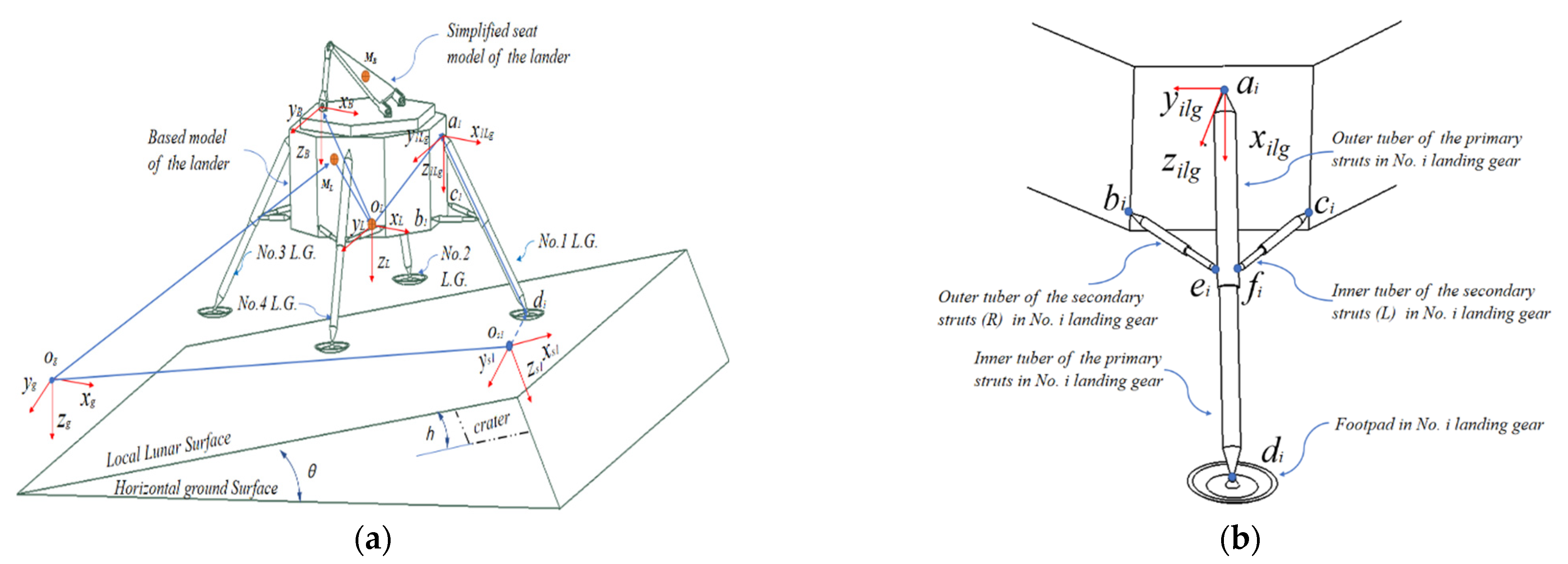
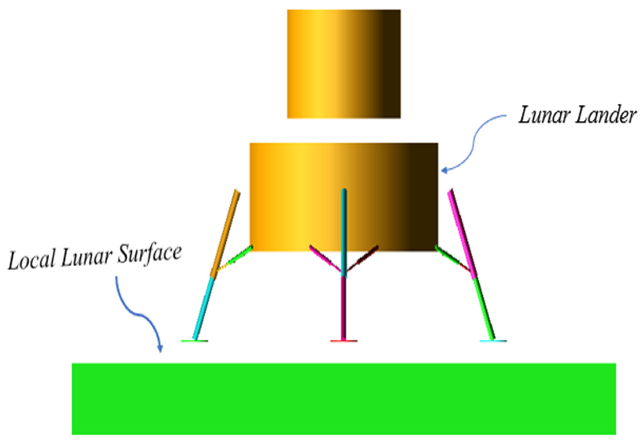
2.1. Model Definition
2.2. Position and Velocity Definition of the Lander
2.3. Dynamics Model of the Simplified Base Model of the Lander
2.4. Dynamic Model of Landing Gear
2.5. Footpad–Ground Bearing Model
2.6. Dynamic Model of the Buffers
2.7. Correction Coefficient η
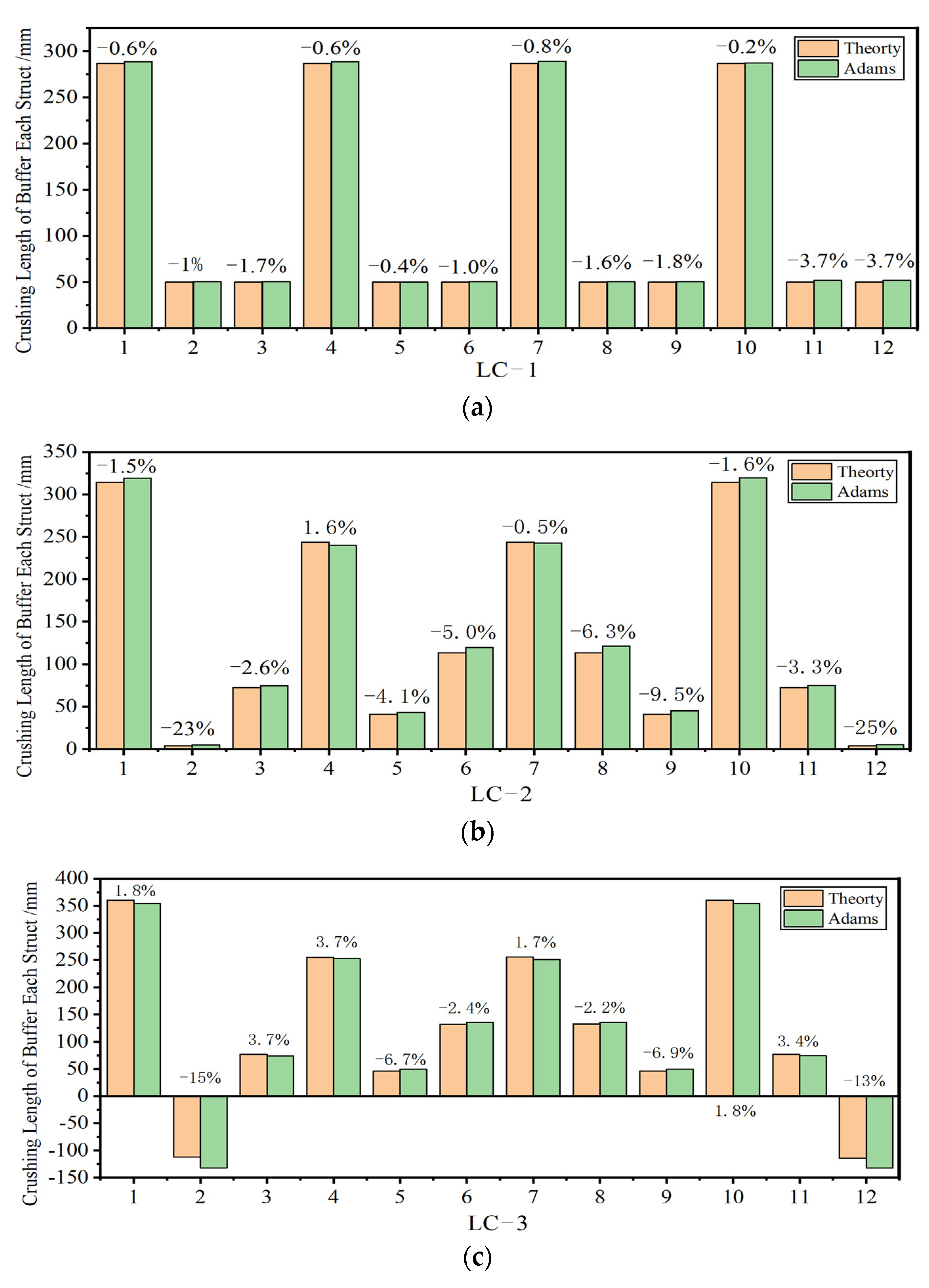
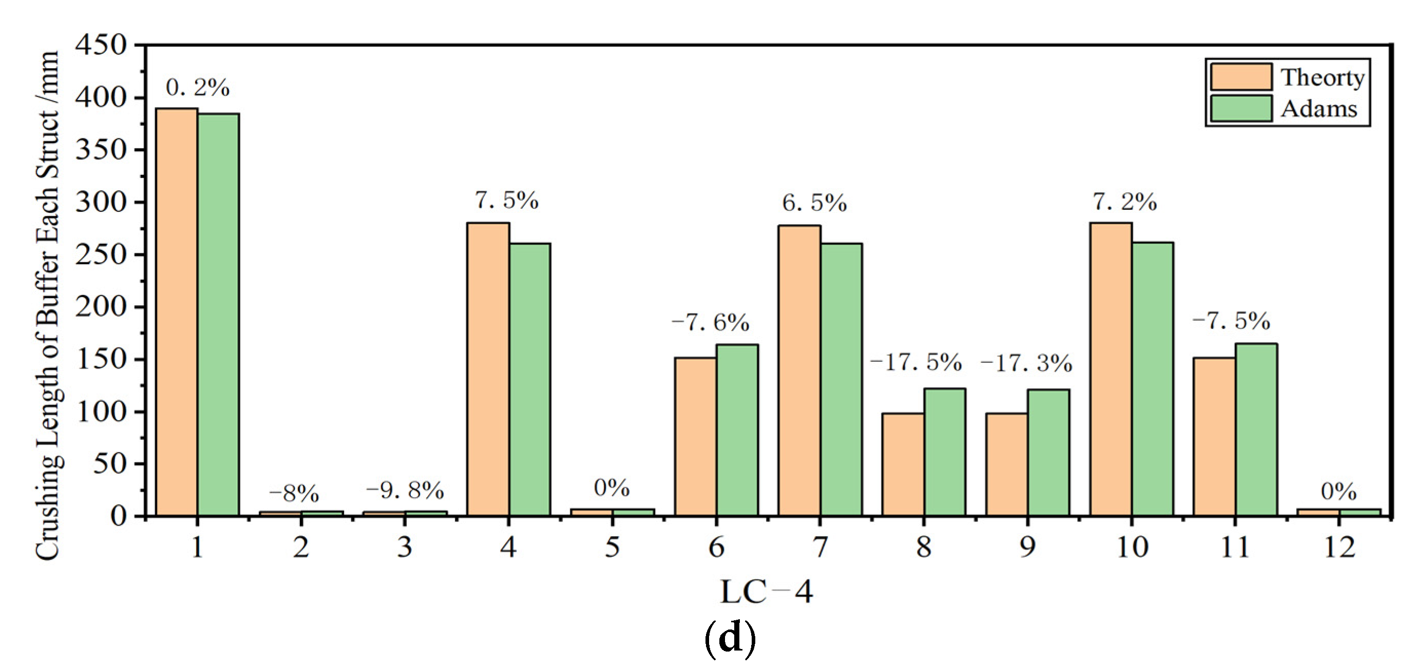
3. Simulation and Model Validation
3.1. Program Flow
3.2. Program Flow
4. Discussions
4.1. Different Kinds of the Footpad–Ground Bearing Models
4.2. Friction Analysis
4.3. Correction Coefficient η
5. Conclusions
Author Contributions
Funding
Data Availability Statement
Conflicts of Interest
Nomenclature
| = | The transformation matrix from the No. i-1 coordinate system to the No. i coordinate system. | |
| = | Unit matrix. | |
| = | Rotation matrix from the No. i-1 coordinate system to the No. i coordinate system in terms of Z-Y-X axis in the Euler angle way . ; ; ; ; | |
| = | Translation matrix relative to the No. i coordinate system. | |
| = | Translation vector relative to the No. i landing gear coordinate system. | |
| = | Translation vector relative to the No. i landing gear coordinate system. | |
| = | Translation vector relative to the No. i landing gear coordinate system. | |
| = | yaw(z) angle of the primary strut in the Euler angle form under the No. i landing gear coordinate system, aiLg-xiLgyiLgziLg. | |
| = | pitch(y) angle of the primary strut in the Euler angle form under the No. i landing gear coordinate system, aiLg-xiLgyiLgziLg. | |
| = | x-component value in the No. i primary strut coordinate system, aiLg-xiLgyiLgziLg. | |
| = | The yaw(z) angle of the primary strut in the Euler angle form under the No. i landing gear coordinate system, biLg-xiLgyiLgziLg and ciLg-xiLgyiLgziLg, respectively. | |
| = | pitch(y) angle of the primary strut in the Euler angle form under the No. i landing gear coordinate system, biLg-xiLgyiLgziLg and ciLg-xiLgyiLgziLg, respectively. | |
| = | x-component value in the No. i secondary strut coordinate system, bi-xilgyilgzilg and ci-xilgyilgzilg, respectively. | |
| = | The velocity matrix of the points ML, di, ei, fi in the global coordinate system, Og-xgygzg. | |
| = | The Jacobian matrices for different mapping relationships. | |
| FLgi | = | The equivalent dynamic force matrix in the No. i landing gear coordinate system, OLgi-xLgiyLgizLgi. |
| Fg | = | The footpad–ground force matrix. |
| FXLgi | = | The x component of the footpad–ground force in the No. i landing gear coordinate system, OLgi-xLgiyLgizLgi. |
| FYLgi | = | The y component of the footpad–ground force in the No. i landing gear coordinate system, OLgi-xLgiyLgizLgi. |
| FZLgi | = | The z component of the footpad–ground force in the No. i landing gear coordinate system, OLgi-xLgiyLgizLgi. |
| = | The equivalent dynamic forces in the primary strut of the No. i landing gear coordinate system. | |
| = | The equivalent dynamic forces in the left secondary strut of the No. i landing gear coordinate system. | |
| = | The equivalent dynamic forces in the right secondary strut of the No. i landing gear coordinate system. | |
| = | x, y, z component of the translation acceleration vector of mass center of the lander in the lander coordinate system. | |
| = | x, y, z component of the angle acceleration vector of mass center of the lander in the lander coordinate system. | |
| = | x, y, z component of the translation velocity vector of mass center of the lander in the global coordinate system. | |
| = | The Euler rates in terms of Euler angles (Z-Y-X) from the global coordinate system to the lander coordinate system. | |
| = | The x, y, z component of the force acting on the mass center of the lander in the lander coordinate system. | |
| = | The x, y, z component of the moment acting on the mass center of the lander in the lander coordinate system. | |
| = | The x, y, z scale component for the moment of momentum in the lander coordinate system. | |
| = | Mass moments of inertia of the lander about x, y, and z axes in the lander coordinate system. | |
| = | The products of the inertia of the lander in the lander coordinate system. | |
| = | The transmission force in the primary strut of the No. i landing gear coordinate system. | |
| = | The transmission force in the left secondary strut of the No. i landing gear coordinate system. | |
| = | The transmission force in the right secondary strut of the No. i landing gear coordinate system. | |
| = | The crushing force of buffer in the primary strut. | |
| = | The tensile crushing force of buffer in the secondary strut. | |
| = | The compression crushing force of buffer in the secondary strut. | |
| = | The remaining driving force in the primary strut of the No. i landing gear coordinate system. | |
| = | The remaining driving force in the left secondary strut of the No. i landing gear coordinate system. | |
| = | The remaining driving force in the left secondary strut of the No. i landing gear coordinate system. | |
| M | = | Generalized mass matrix of each landing gear system. |
| = | Generalized coordination vectors matrix, | |
| = | The generalized acceleration vectors matrix, | |
| Φq | = | The Jacobi matrix of the constraint equation (Equation (7)). |
| λ | = | Lagrange multiplier column matrix. |
| γ | = | Constraint matrix. |
| = | The remaining driving force matrix in the generalized coordinate system. | |
| Flun | = | Footpad–ground contact force. |
| n | = | Exponential coefficient of the penetration depth. |
| µ | = | Frictional coefficient of the contact force. |
| Kg, Cg | = | Penetration stiffness and damping coefficient of the footpad–ground model. |
| = | x, y, z component of the displacement of the No. i footpad in the lunar surface coordinate system. | |
| = | x, y, z component of the translation velocity of the No. i footpad in the lunar surface coordinate system. | |
| D, D1, D2 | = | Defined displacement parameters in contact model. |
| = | Contact parameter. | |
| ,, | = | Crushing acceleration, velocity, and displacement of the buffer. |
| a, b, c, d | = | Coefficients of inertia, viscosity, stiffness, and constant resistance of the buffer. |
| F1, F2 | = | Crush forces of the first and second step of the buffer in the primary strut. |
| F3 | = | Transmission force after the AL-honeycomb is crushed. |
| s0 | = | Initial length of the primary strut. |
| s1, s2 | = | Lengths of the primary strut when the first and second step foam crush are done. |
| shismin | = | Minimum length of the primary strut before the currently measured time. |
| sc1, st1 | = | Length value of the secondary strut when the compaction buffer or the tension buffer crush are done. |
| Fcom, FTen | = | Compaction and tension force of the buffer in the secondary struts. |
| Fcom1, FTen1 | = | Compaction and tension transmission force of the buffer in the secondary struts after the AL-honeycomb is crushed. |
| = | Maximum length of the secondary strut before the currently measured time. | |
| = | Minimum length of the secondary strut before the currently measured time. | |
| = | Total normal contact force acted upon the No. i primary strut by the relative secondary struts. | |
| = | y component of the contact force matrix in the No. i primary strut coordinate system. | |
| = | z component of the contact force matrix in the No. i primary strut coordinate system. | |
| = | Contact force matrix acted upon the No. i primary strut and by the secondary struts in the No. i primary strut coordinate system, di-xilgyilgzilg. | |
| η | = | Correction coefficient of the contact between the outer and inner tube in the primary strut. |
| µ1 | = | Friction factor of the contact between the outer and inner tube in the primary strut. |
| η1 | = | Correction factor accounts for the changing length of the landing gear during the soft-landing process. |
| η2 | = | Correction factor takes into consideration the effect on the contact pressure distribution. |
| NA | = | Lateral force caused by the upper contact action of the tubes. |
| NB | = | Lateral force caused by the below contact action of the tubes. |
| μk | = | Kinetic coefficient of friction. |
| FC | = | The magnitude of friction force. |
| FS | = | Static friction force. |
| FD | = | Dynamic friction force. |
| Fe | = | External tangential force. |
| v | = | The relative tangential velocity of the contacting surfaces. |
| vo | = | Stiction velocity. |
| p | = | Contact pressure. |
| pm | = | Maximum contact pressure. |
| = | Contact angle between the outer and inner tube in the primary strut. | |
| l | = | Arc length of the contact between the outer and inner tube in the primary strut. |
| lR | The inner radius of the outer tube in the primary strut. | |
| = | Constraint function in the No. i landing gear. | |
| = | Generalized coordinate displacement and velocity by numerical integration at time step tn+1. | |
| Correction displacement and velocity item at time step tn+1. | ||
| Subscripts | ||
| Soft landing | Any type of spacecraft landing that does not result in significant damage to or destruction of the vehicle or its payload. | |
| MC | Center of mass. | |
| C.L. | Coordinate location. | |
| No. | Number order. | |
| C.S. | Coordinate system. | |
| L.G. | Landing gear. | |
| LC | Load case. | |
| Pri. Strut | Primary strut. | |
| Sec. Strut | Secondary strut. |
References
- China Unveils Preliminary Plan on Manned Lunar Landing. Available online: http://english.www.gov.cnnews/202305/29/content_WS64748c46c6d03ffcca6ed781.html (accessed on 12 July 2023).
- Yang, J.; Wu, Q.; Yu, D.; Jiang, S.; Xu, Z.; Cui, P. Preliminary Study on Key Technologies for Construction and Operation of Robotics Lunar Scientific Base. J. Deep. Space Explor. 2020, 7, 111–117. (In Chinese) [Google Scholar]
- Lin, R.; Guo, W.; Zhao, C.; He, M. Conceptual design and analysis of legged landers with orientation capability. Chin. J. Aeronaut. 2023, 36, 171–183. [Google Scholar] [CrossRef]
- Hu, Y.; Guo, W.; Lin, R. An Investigation on the Effect of Actuation Pattern on the Power Consumption of Legged Robots for Extraterrestrial Exploration. IEEE Trans. Robot. 2023, 39, 923–940. [Google Scholar] [CrossRef]
- Zhou, J.; Ma, H.; Chen, J.; Jia, S.; Tian, S. Motion characteristics and gait planning methods analysis for the walkable lunar lander to optimize the performances of terrain adaptability. Aerosp. Sci. Technol. 2023, 132, 44–46. [Google Scholar] [CrossRef]
- John, F.C. After LM: NASA Lunar Lander Concepts beyond Apollo. Available online: https://ntrs.nasa.gov/citations/20190031985 (accessed on 22 June 2023).
- Rogers, W.F. Apollo Experience Report-Lunar Module Landing Gear Subsystem. Available online: https://ntrs.nasa.gov/citations/19720018253 (accessed on 22 June 2023).
- Liang, D.; Chai, H.; Chen, T. Overview of Lunar Lander Soft Landing Dynamic Modeling and Analysis. Spacecr. Eng. 2011, 20, 104–112. (In Chinese) [Google Scholar]
- Lavender, R.E. Equations for Two-Dimensional Analysis of Touchdown Dynamics of Spacecraft with Hinged Legs Including Elastic, Damping, and Crushing Effects. Available online: https://ntrs.nasa.gov/citations/19660014379 (accessed on 22 June 2023).
- Alderson, R.G.; Wells, D.A. Surveyor Lunar Touchdown Stability Study Final Report, July 1965–July 1966. Available online: https://ntrs.nasa.gov/citations/19670003854 (accessed on 22 June 2023).
- Zupp, G.A.; Doiron, H.H. A Mathematical Procedure for Predicting the Touchdown Dynamics of a Soft-Landing Vehicle. Available online: https://ntrs.nasa.gov/citations/19710007293 (accessed on 22 June 2023).
- Maeda, T.; Ozaki, T.; Hara, S.; Matsui, S. Touchdown Dynamics of Planetary Lander with Translation–Rotation Motion Conversion Mechanism. J. Spacecr. Rocket. 2017, 54, 973–980. [Google Scholar] [CrossRef]
- Wan, J. Research on Soft Landing Dynamic Analysis and Several Key Technologies of Lunar Lander. Ph.D. Thesis, Nanjing University of Aeronautics and Astronautics, Nanjing, China, 2010. [Google Scholar]
- Yue, S.; Lin, Q.; Zheng, G.; Du, Z. Touchdown Dynamics of Planetary Lander with Translation–Rotation Motion Conversion Mechanism. Chin. J. Aeronaut. 2022, 35, 156–172. [Google Scholar] [CrossRef]
- Yin, K.; Sun, Q.; Gao, F.; Zhou, S. Lunar surface soft-landing analysis of a novel six-legged mobile lander with repetitive landing capacity. Proc. Inst. Mech. Eng. Part C J. Mech. Eng. Sci. 2021, 236, 1214–1233. [Google Scholar] [CrossRef]
- Lin, Q.; Ren, J. Investigation on the Horizontal Landing Velocity and Pitch Angle Impact on the Soft-Landing Dynamic Characteristics. Int. J. Aerosp. Eng. 2022, 2022, 1214–1233. [Google Scholar] [CrossRef]
- Yin, C.; Quan, Q.; Tang, D.; Deng, Z. Landing of the asteroid probe with three-legged cushioning: Planar asymmetric dynamics and safety margin. Adv. Space Res. 2023, 71, 2075–2094. [Google Scholar] [CrossRef]
- Dong, Y.; Ding, J.; Wang, C.; Wang, H.; Liu, X. Soft landing stability analysis of a Mars lander under uncertain terrain. Chin. J. Aeronaut. 2022, 35, 377–388. [Google Scholar] [CrossRef]
- Jeffrey, A.; Goldman, D.I. Robophysical study of jumping dynamics on granular media. Nat. Phys. 2016, 12, 278–283. [Google Scholar]
- Wu, S.; Wang, Y.; Hou, X.; Xue, P.; Long, L. Research on Theoretical Model of Vertical Impact of Foot Pad on Lunar Soil. Manned Spacefl. 2016, 26, 135–141. (In Chinese) [Google Scholar]
- Nelson, R.C. Flight Stability and Automatic Control, 1st ed.; McGraw-Hill College: New York, NY, USA, 1989; pp. 50–90. [Google Scholar]
- Craig, J.J. Introduction to Robotics Mechanics and Control, 3rd ed.; Pearson Education, Inc.: River Street Hoboken, NJ, USA, 2005; pp. 40–80. [Google Scholar]
- Yu, Q.; Chen, I.-M. A direct violation correction method in numerical simulation of constrained multibody systems. Comput. Mech. 2000, 26, 52–57. [Google Scholar] [CrossRef]
- Hong, J. Computational Dynamics of Multibody Systems, 1st ed.; Higher Education Press: Beijing, China, 1999; pp. 360–380. [Google Scholar]
- Chen, H. Investigation on Energy-Absorption Nanomaterials for Lunar Lander and Analysis on Soft-Landing Performance. Ph.D. Thesis, Nanjing University of Aeronautics and Astronautics, Nanjing, China, 2017. [Google Scholar]
- Zhao, D.; Liu, Y. Improved Damping Constant of Hertz-Damp Model for Pounding between Structures. Math. Probl. Eng. 2016, 2016, 52–57. [Google Scholar] [CrossRef]
- Paulo, F.; Margarida, M.; Silva, M.T.; Martins, J.M. On the continuous contact force models for soft materials in multibody dynamics. Multibody Syst. Dyn. 2011, 25, 357–375. [Google Scholar]
- Jankowski, R. Non-linear viscoelastic modelling of earthquake-induced structural pounding. Earthq. Eng. Struct. Dyn. 2005, 34, 595–611. [Google Scholar] [CrossRef]
- Jankowski, R. Analytical expression between the impact damping ratio and the coefficient of restitution in the non-linear viscoelastic model of structural pounding. Earthq. Eng. Struct. Dyn. 2005, 35, 517–524. [Google Scholar] [CrossRef]
- Hunt, K.H.; Crossley, F.R.E. Coefficient of Restitution Interpreted as Damping in Vibroimpact. J. Appl. Mech. 1975, 42, 440–445. [Google Scholar] [CrossRef]
- Wang, G.; Ma, D.; Liu, Y.; Liu, C. Coefficient of Restitution Interpreted as Damping in Vibroimpact. Chin. J. Theor. Appl. Mech. 2022, 54, 3239–3266. [Google Scholar]
- Filipe, M.; Paulo, F.; Pimenta Claro, J.C.; Lankarani, H.M. Modeling and analysis of friction including rolling effects in multibody dynamics: A review. Nonlinear Dyn. 2016, 45, 223–244. [Google Scholar]
- Filipe, M.; Paulo, F.; Pimenta Claro, J.C.; Lankarani, H.M. A survey and comparison of several friction force models for dynamic analysis of multibody mechanical systems. Nonlinear Dyn. 2016, 86, 1407–1443. [Google Scholar]


| Mass Property | C.L. of Points | Crush Force of Buffers | Contact Property | ||||||
|---|---|---|---|---|---|---|---|---|---|
| Pri. Strut | Sec. Strut | ||||||||
| Ix | 8.18 × 10⁴ | (3.89, 0, −2.18) | F1 | 78,000 | Fcom | 43,000 | Kg | (1000)1.5 ×10⁵ | |
| Iy | 8.18 × 10⁴ | (3.37, 1.23, −1.01) | F2 | 156,000 | Ften | 30,000 | Cg | 10,000 | |
| Iz | 8.17 × 10⁴ | (3.37, −1.23, −1.01) | 0.2 | 0.27 | 0.0001 | ||||
| Mass | 1.6 × 10⁴ | (5.48, 0, 0.94) | 0.475 | 0.27 | us | 0.4/0.4 | |||
| (4.65, 1.09, −0.505) | 0.1 | ||||||||
| (4.65, −1.09, 0.505) | 0.1 | ||||||||
| MC | (0, 0, −3.818) | η | 0 | ||||||
| vs | 0.1 | ||||||||
| vd | 1 | ||||||||
| Load Cases | Velocity m/s | Attitude Angles /Deg | Lunar Surface Slope Angle /Deg | |
|---|---|---|---|---|
| Vertical | Horizontal | |||
| LC-1 | 4 | −0 | 0/0/0 | 0 |
| LC-2 | 4 | 1 | 45/0/0 | 0 |
| LC-3 | 4 | 1 | 45/−4/0 | 8 |
| LC-4 | 4 | 1 | 0/4/0 | 8 |
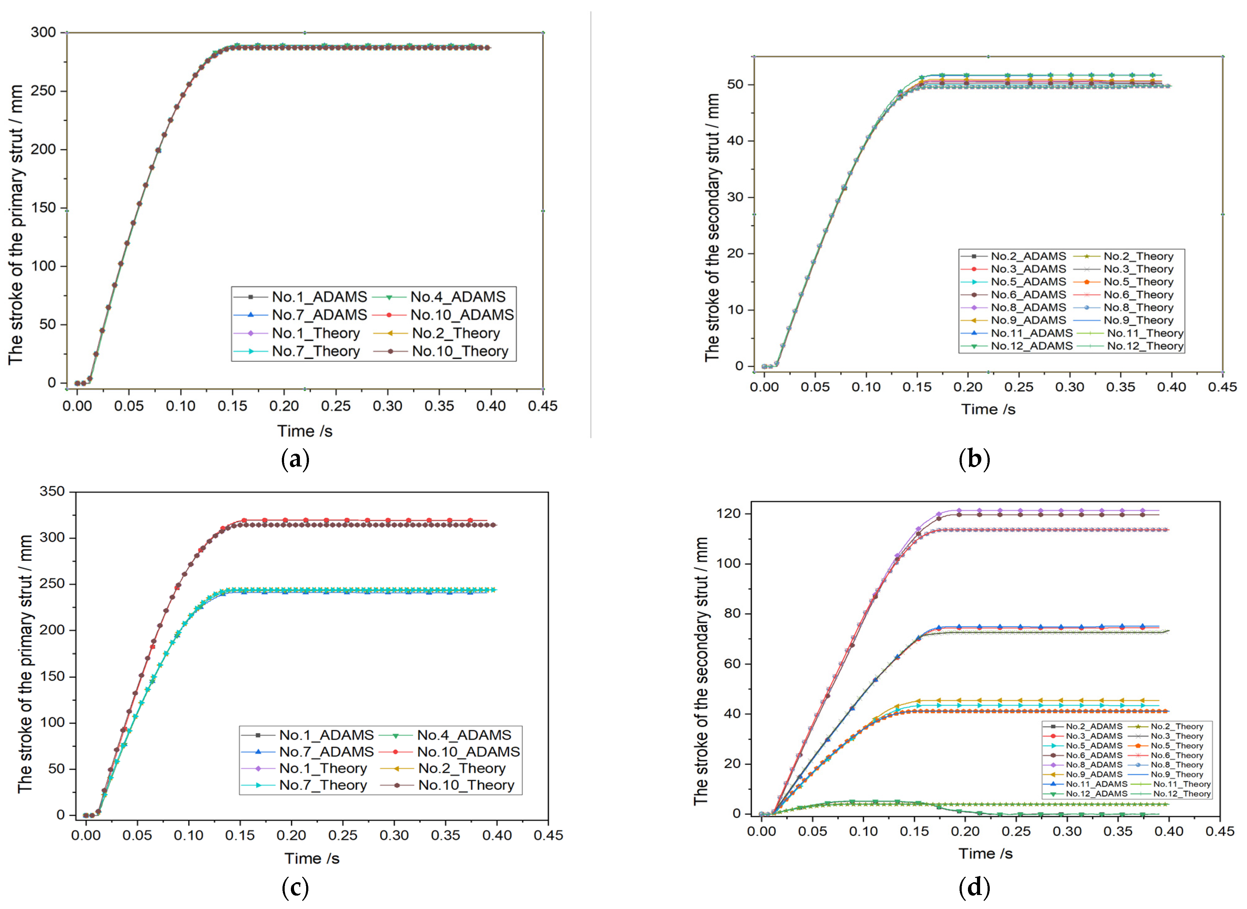
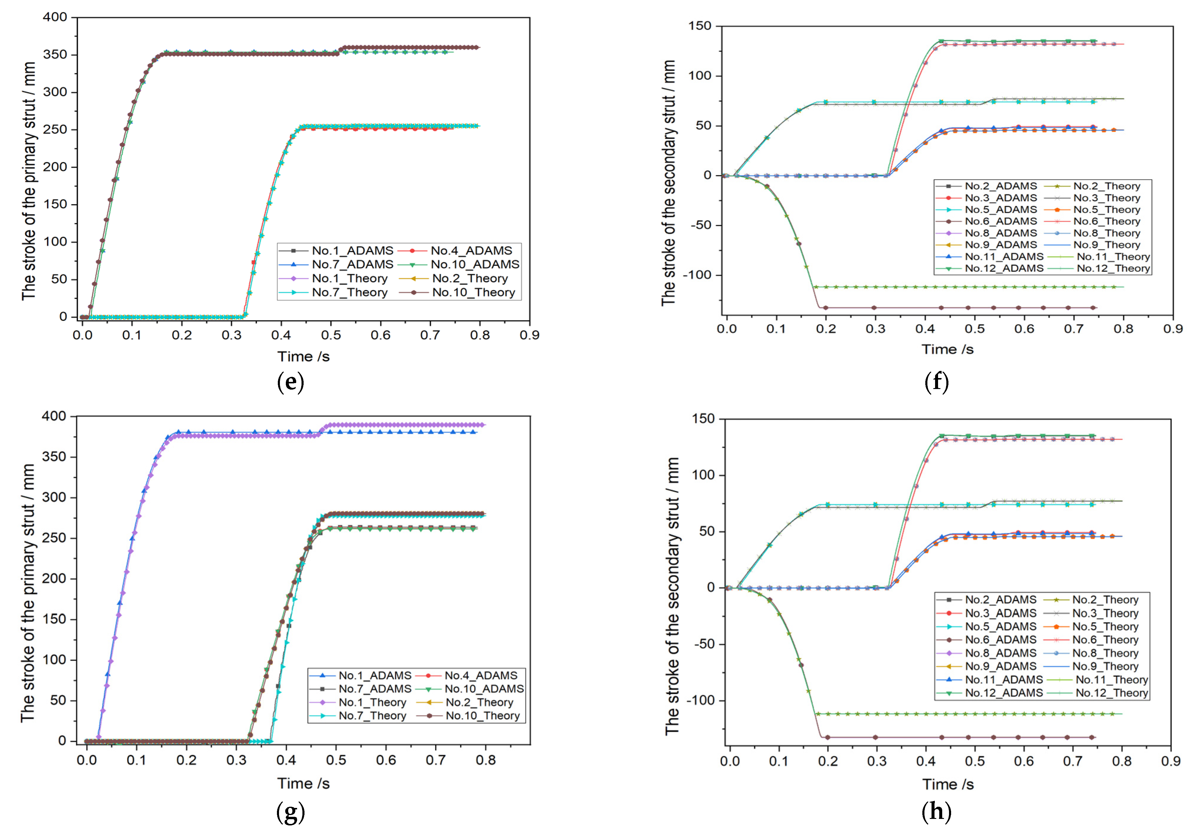
| No. | LC-1 | LC-2 | LC-3 | LC-4 | ||||||||
|---|---|---|---|---|---|---|---|---|---|---|---|---|
| Theory | Adams | Dev | Theory | Adams | Dev | Theory | Adams | Dev | Theory | Adams | Dev | |
| 1 1 | 287.0 | 288.8 | −1.8 | 314.3 | 319 | −4.7 | 360.3 | 354.1 | 9.8 | 390.0 | 385.0 | 5.0 |
| 2 2 | 49.8 | 50.3 | −0.5 | 3.9 | 5.1 | −1.2 | −112.1 | −132.2 | 19.1 | 4.4 | 5.0 | −0.6 |
| 3 3 | 49.8 | 50.7 | −0.5 | 72.6 | 74.5 | −1.9 | 77.0 | 74.2 | 3.8 | 4.4 | 5.1 | −0.7 |
| 4 4 | 287.0 | 288.7 | −0.7 | 244.0 | 240.0 | 4.0 | 255.3 | 252.7 | 2.6 | 280.6 | 261.0 | 19.6 |
| 5 5 | 49.8 | 50.0 | −0.2 | 41.2 | 43.5 | −1.8 | 46.1 | 49.4 | −3.3 | 7.3 | 7.3 | 0 |
| 6 6 | 49.8 | 50.3 | −0.5 | 113.7 | 119.7 | 6.0 | 132.3 | 135.6 | 3.3 | 151.9 | 164.4 | −13.5 |
| 7 7 | 287 | 289.2 | 2.0 | 244.0 | 242.9 | 1.1 | 255.4 | 251.2 | 4.2 | 277.9 | 261.0 | 16.9 |
| 8 8 | 49.8 | 50.6 | −0.8 | 113.7 | 121.4 | −7.7 | 132.6 | 135.6 | 3.0 | 98.3 | 121.9 | −20.9 |
| 9 9 | 49.8 | 50.7 | −0.9 | 41.2 | 45.5 | −4.3 | 46.0 | 49.4 | 3.0 | 98.3 | 121.5 | −20.9 |
| 10 10 | 287.0 | 287.5 | 2.0 | 314.2 | 319.5 | −5.3 | 360.3 | 354.0 | 6.3 | 280.6 | 261.6 | 19.0 |
| 11 11 | 49.8 | 51.7 | −1.9 | 72.6 | 75.1 | −2.5 | 77.0 | 74.5 | 2.5 | 151.9 | 165.0 | −14.1 |
| 12 12 | 49.8 | 51.7 | −1.9 | 3.9 | 5.2 | −1.3 | −114.7 | −132.2 | 18.5 | 7.3 | 7.3 | 0 |
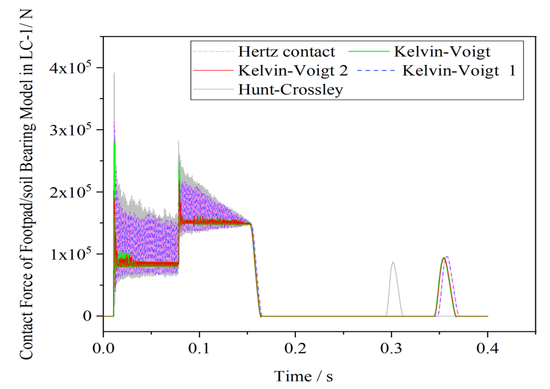
| Contact Model Types | Equation | Contact Model | Equation |
|---|---|---|---|
| Hertz contact | Hertz contact + linear damping | ||
| Hertz contact + step damping | Hertz contact + bilinear damping | ||
| Hertz contact + hysteresis damping 1 |
| Model Name 1 | Model Type | Parameter Defined in the Model |
|---|---|---|
| Hertz contact | Hertz contact | K = (1000) 1.5 × 1.0 × 105, n = 1.5 |
| Kelvin–Voigt model | Hertz contact + linear damping factor | K = (1000)1.5 × 1.0 × 105, D = 10 × 1000, n = 1.5 |
| Kelvin–Voigt 1 | Hertz contact + step damping factor | K = (1000)1.5 × 1.0 × 105, D = 10 × 1000, n = 1.5 |
| Kelvin–Voigt 2 | Hertz contact + bilinear damping factor | K = (1000)1.5 × 1.0 × 105, D1 = 10 × 1000, D2 = 10 × 1000, n = 1.5 |
| Hunt–Crossley | Hertz contact + hysteresis damping factor | K = (1000)1.5 × 1.0 × 105, n = 1.5 |
| Info. | No. | Base Result | Hertz | Kelvin–Voigt | Kelvin–Voigt 1 | Kelvin–Voigt 2 | Hunt–Crossley |
|---|---|---|---|---|---|---|---|
| LC-1 | 1 1 | 287.0 | 288.8 | 287.3 | 288.8 | 287.0 | 289.8 |
| 2 2 | 49.8 | 50.5 | 49.8 | 50.5 | 49.8 | 50.7 | |
| 3 3 | 49.8 | 50.5 | 49.8 | 50.5 | 49.8 | 50.7 | |
| LC-2 | 4 4 | 314.0 | 312.9 | 314.1 | 311.4 | 314.0 | 317.7 |
| 5 5 | 3.9 | 6.3 | 4.0 | 6.4 | 3.9 | 12.1 | |
| 6 6 | 41.1 | 41.6 | 41.2 | 41.8 | 41.1 | 41.6 | |
| 7 7 | 244.0 | 244.5 | 244.1 | 244.9 | 244.0 | 244.1 | |
| 8 8 | 113.6 | 112.7 | 113.9 | 114.0 | 113.6 | 109.1 | |
| 9 9 | 73.4 | 74.2 | 72.7 | 75.1 | 73.4 | 74.0 |
| Friction Model Types 1 | Calculation Equations 2 | The Change Rule Figures |
|---|---|---|
| The static Coulomb friction model |  | |
| The static Coulomb friction model with viscous effect | 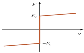 | |
| The regularized Coulomb friction model | 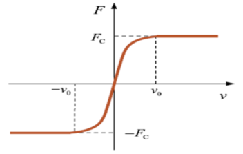 | |
| The stiction + dynamic Coulomb model | 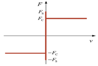 | |
| The stiction + Stribeck + Coulomb + viscous friction model | 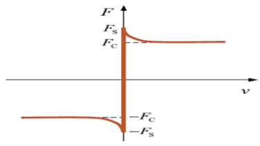 | |
| The stiction + modified Stribeck + Coulomb + viscous friction model | 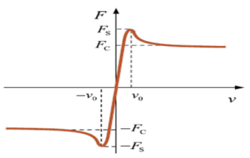 |
| No. | Friction Model | Parameter |
|---|---|---|
| TY-1 | Static Coulomb friction | = 0.4 |
| TY-2 | Static Coulomb friction model with viscous effect | = 0.4; = 100 |
| TY-3 | Regularized Coulomb friction | = 0.1 m/s; = 0.4 |
| TY-4 | Stiction + dynamic Coulomb | = 0.4 |
| TY-5 | Stiction + Stribeck + Coulomb + viscous friction | = 1 m/s; |
| TY-6 | Stiction + modified Stribeck + Coulomb + viscous friction |
| Measure Option | Base Result | TY-1 | TY-2 | TY-3 | TY-4 | TY-5 | TY-6 | |
|---|---|---|---|---|---|---|---|---|
| LC-1 | 1 1 | 287.0 | 295.1 | 295.0 | 290.6 | 295.1 | 295.1 | 290.2 |
| 2 2 | 49.8 | 48.4 | 48.4 | 49.3 | 48.4 | 48.4 | 49.5 | |
| 3 3 | 49.8 | 48.4 | 48.4 | 49.3 | 48.4 | 48.4 | 49.5 | |
| LC-2 | 4 4 | 314.0 | 368.3 | 324.4 | 316.0 | 368.3 | 323.7 | 313.4 |
| 5 5 | 4.0 | 10.2 | 7.4 | 7.2 | 10.2 | 7.4 | 6.8 | |
| 6 6 | 41.1 | 39.6 | 39.8 | 40.9 | 39.6 | 39.8 | 41.2 | |
| 7 7 | 244.0 | 252.7 | 249.0 | 245.3 | 252.7 | 249.1 | 245.5 | |
| 8 8 | 113.6 | 92.4 | 106.0 | 109.9 | 92.4 | 107.0 | 111.8 | |
| 9 9 | 73.4 | 62.0 | 71.8 | 75.7 | 62.0 | 73.2 | 76.4 |
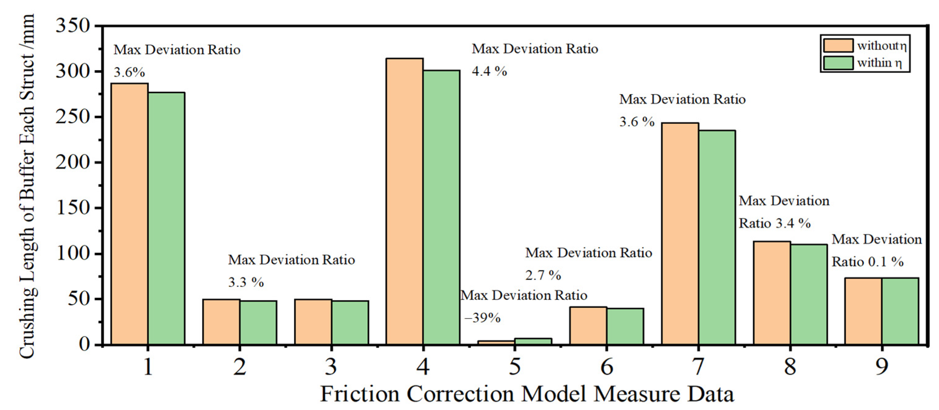
| Info. | Measure Options | /mm | /mm | Error/% |
|---|---|---|---|---|
| LC-1 | 1 1 | 287.0 | 276.9 | 3.6 |
| 2 2 | 49.8 | 48.2 | 3.3 | |
| 3 3 | 49.8 | 48.2 | 3.3 | |
| LC-2 | 4 4 | 314.0 | 300.9 | 4.4 |
| 5 5 | 4.0 | 6.6 | −39.0 | |
| 6 6 | 41.1 | 40.0 | 2.7 | |
| 7 7 | 243.7 | 235.2 | 3.6 | |
| 8 8 | 113.6 | 109.9 | 3.4 | |
| 9 9 | 73.4 | 73.3 | 0.1 |
Disclaimer/Publisher’s Note: The statements, opinions and data contained in all publications are solely those of the individual author(s) and contributor(s) and not of MDPI and/or the editor(s). MDPI and/or the editor(s) disclaim responsibility for any injury to people or property resulting from any ideas, methods, instructions or products referred to in the content. |
© 2023 by the authors. Licensee MDPI, Basel, Switzerland. This article is an open access article distributed under the terms and conditions of the Creative Commons Attribution (CC BY) license (https://creativecommons.org/licenses/by/4.0/).
Share and Cite
Wang, Z.; Chen, C.; Chen, J.; Zheng, G. 3D Soft-Landing Dynamic Theoretical Model of Legged Lander: Modeling and Analysis. Aerospace 2023, 10, 811. https://doi.org/10.3390/aerospace10090811
Wang Z, Chen C, Chen J, Zheng G. 3D Soft-Landing Dynamic Theoretical Model of Legged Lander: Modeling and Analysis. Aerospace. 2023; 10(9):811. https://doi.org/10.3390/aerospace10090811
Chicago/Turabian StyleWang, Zhiyi, Chuanzhi Chen, Jinbao Chen, and Guang Zheng. 2023. "3D Soft-Landing Dynamic Theoretical Model of Legged Lander: Modeling and Analysis" Aerospace 10, no. 9: 811. https://doi.org/10.3390/aerospace10090811
APA StyleWang, Z., Chen, C., Chen, J., & Zheng, G. (2023). 3D Soft-Landing Dynamic Theoretical Model of Legged Lander: Modeling and Analysis. Aerospace, 10(9), 811. https://doi.org/10.3390/aerospace10090811