1. Introduction
The work presented in this paper is part of the European H2020 ASCenSIon project. In recent years, reusable space system technologies have been demonstrated to be one of the most effective solution to reduce the costs of access to space [
1]. The re-flight capability and the wide range of missions demanded by a reusable space vehicle drive the necessity of a dedicated missionisation tool to minimise the tailoring effort among each flight. In this context, missionisation aims at evaluating the mission performance to achieve the optimal adaptation of the mission analysis and GNC solution accounting for the mission and system requirements of a specific mission.
This paper focuses on the mission analysis of the propellant-optimal return trajectory of a Vertical Landing Reusable Launch Vehicle (VL-RLV) [
2,
3]. In particular, the goal is to obtain performance envelopes and the mission feasibility region by considering a wide range of conditions at MECO without violating propellant budget, aerothermal-mechanical loads, and path constraints. The analysis aims at estimating the propellant needed to perform RTLS and DRL recoveries for a representative variability of the MECO conditions. The objective of these maps is to assess the launcher flexibility and capabilities, as well as estimating the propellant consumption concerning different mission scenarios. This analysis represents a crucial tool for an efficient missionisation of the mission analysis solution for a specific mission. Characteristics conditions for LEO and GTO missions, indeed, can be mapped in terms of velocity and Flight-Path-Angle (FPA) at MECO [
4,
5].
The launch vehicle considered in this study is a small-lift launcher with similar features to Electron by Rocket Lab [
6], even if the methodology can be applied to a launch vehicle of any size. The analysis considers a propulsive descent and landing without additional drag devices such as parachutes and parafoil. The choice of employing such a category of launch vehicle is dictated by three reasons. The first one is because diverse programs are carrying out analysis with small-lift launchers such as Ariane Next and Callisto [
1,
7,
8]. The second reason is that a large number of small-lift launch vehicle startups are rising, that are considering the reusability an option to lower the costs [
9]. The third reason is due to the fact that the literature is plenty of analysis regarding reusable heavy and medium-lift rockets, while it is relatively poor regarding small-lift vehicles [
4].
A dedicated missionisation tool developed within ASCenSIon is exploited to perform the analysis and to build the maps [
10]. A direct collocation method and a gradient-based optimiser are used to solve a set of multi-phase trajectory optimisation problems characterised by different MECO conditions. One bottleneck faced with this analysis is the high computational effort in solving the family of optimal control problem. In the literature there are different solutions to cope with this aspect. One option foresees the employment of convexification techniques to solve the problem in real-time as presented in [
2,
3,
11]. These sophisticated algorithms are largely used and studied in the context of the on-board guidance of reusable launchers. However, an unique multiphase end-to-end formulation of the minimum-propellant problem with these methods is not trivial, since the formulation of the original problem must be modified. In this context, S. You proposed alearning-based and theory-supported optimal control method in [
12], but also in this case, it only applies to the landing phase. Alternatively, interesting options are given by the database-driven [
13] and metamodeling techniques [
14], which estimates the output of a generic problem by using a surrogate model that can be evaluated instantaneously.
In this work, in particular, a Gaussian Radial Basis Functions (RBFs) metamodel is used. A predefined number of optimal control problems are solved, and RBFs are employed to create the surrogate of the original problem and estimates the output [
14]. Consequently, the missionisation tool evaluates the metamodel in the domain of interest to build the performance maps. The initial population used to solve the optimal control problem has been randomly generated with a Latin Hypercube Sampling method.
The structure of this paper is organised as follows:
Section 2 gives an overview of the Mission Analysis and GNC missionisation tool.
Section 3 reports the RTLS and DRL mission scenarios and the mathematical models used to simulate the problem. Moreover, it gives an insight into the Flying Qualities Analysis (FQA).
Section 4 describes the optimisation problem for RTLS and DRL.
Section 5 outlines the test cases and shows the results, while
Section 6 underlines the conclusion.
2. Missionisation Tool Overview
The tool has been developed using
MATLAB (
https://www.mathworks.com/products/matlab.html), following a modular and structured approach. The primary goal was to create software that is user-friendly for setup, maintenance, and continuous improvement. This software is designed to be versatile, accommodating a wide range of applications. The underlying concept is to provide a multidisciplinary tool that can be utilised at various stages of the design process, allowing the user to tailor the level of accuracy and complexity to their specific needs.
In
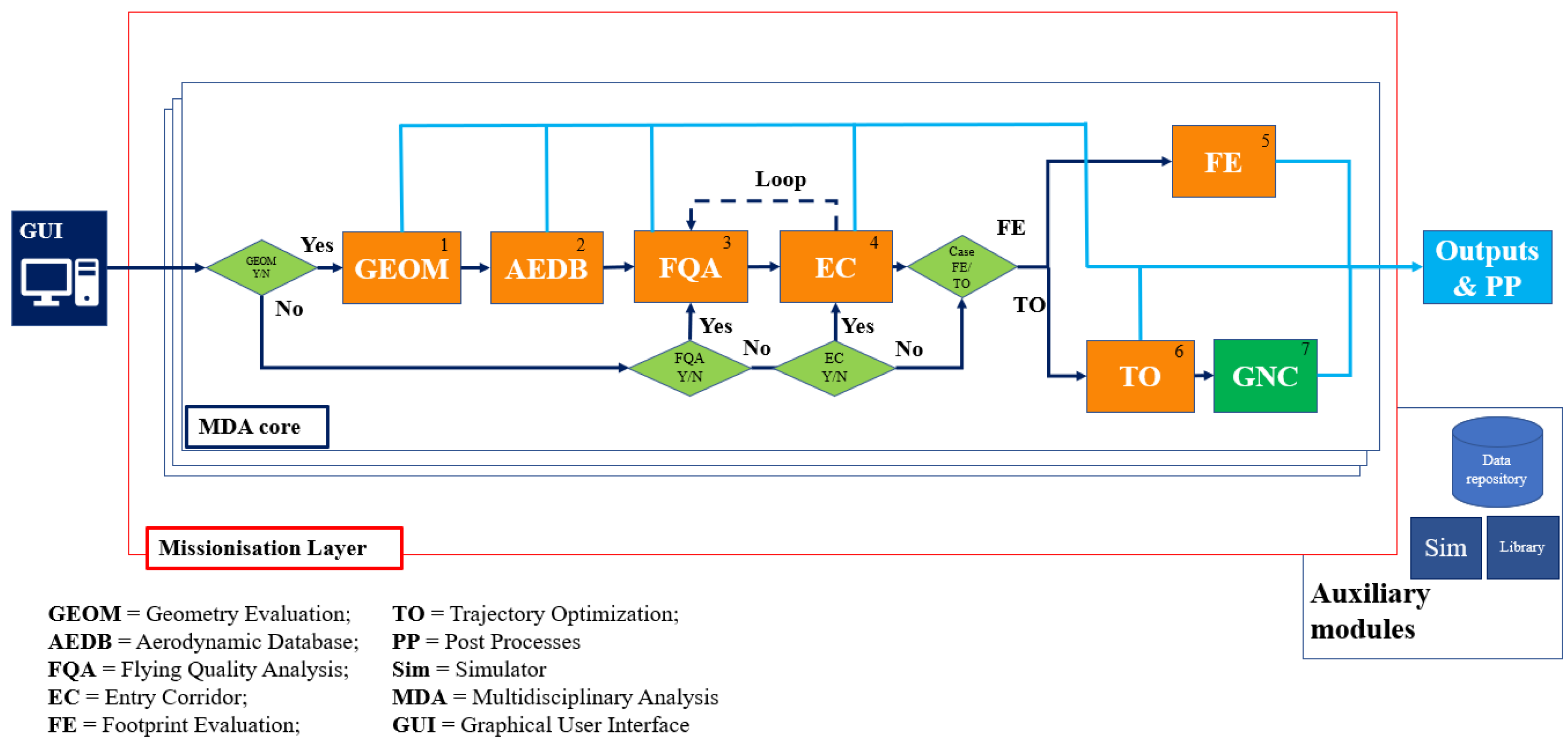
Figure 1, it can be observed the high-level architecture of the missionisation tool. This tool comprises three primary modules and two submodules. The three main modules consist of the User Interface, the MDA core, and the Missionisation Layer. Additionally, there are two submodules, namely the Post-Process unit and the auxiliary functions.
The main module of the software is the MDA core. It comprehends a minimum set of disciplines to evaluate the necessary performance in re-entry mission design:
Geometry and Mass Estimation Tool (GEOM): This tool estimates the reference surface and dry mass of the vehicle using a minimal set of geometric parameters [
15].
Aerodynamic Database Tool (AEDB): It provides a representative aerodynamic database (AEDB) for the vehicle, if needed.
Flying Qualities Analysis Tool (FQA): FQA calculates the domain within which the vehicle can maintain a stable, trimmed configuration during flight.
Entry Corridor Analysis Tool (EC): EC assesses the flight domain in which the vehicle can operate without exceeding aerothermal and mechanical load limits.
Footprint Evaluation Tool (FE): FE computes the vehicle’s feasible range capability [
16].
Trajectory Optimisation Tool (TO): TO solves single or multi-phase optimal control problems and generates an end-to-end mission profile.
Guidance, Navigation, and Control Tool (GNC): GNC facilitates the automatic translation of TO tool outputs into a format required by external GNC models.
As shown in
Figure 1, these disciplines are intricately interconnected, particularly in terms of their input/output relationships. The input parameters of each discipline are derived from the outputs of previous ones. The MDA core enables the execution of the intricate multidisciplinary analyses needed for missionisation in both MA and GNC. It accomplishes this by considering the interdependencies among variables and disciplines within a single, integrated tool. For a more detailed overview, the reader is reffered to [
10].
The external layer of the tool is constituted by the Missionisation Layer, which exploits the capabilities of the MDA core for various objectives. These analyses span from conducting a single MDA cycle to carrying out parametric and preliminary sensitivity analyses. Furthermore, it supports the parametric optimisation of mission and system parameters, as defined by the user. This last application makes use of Multidisciplinary Design Optimisation and metamodeling techniques, as reported in
Section 4.2.
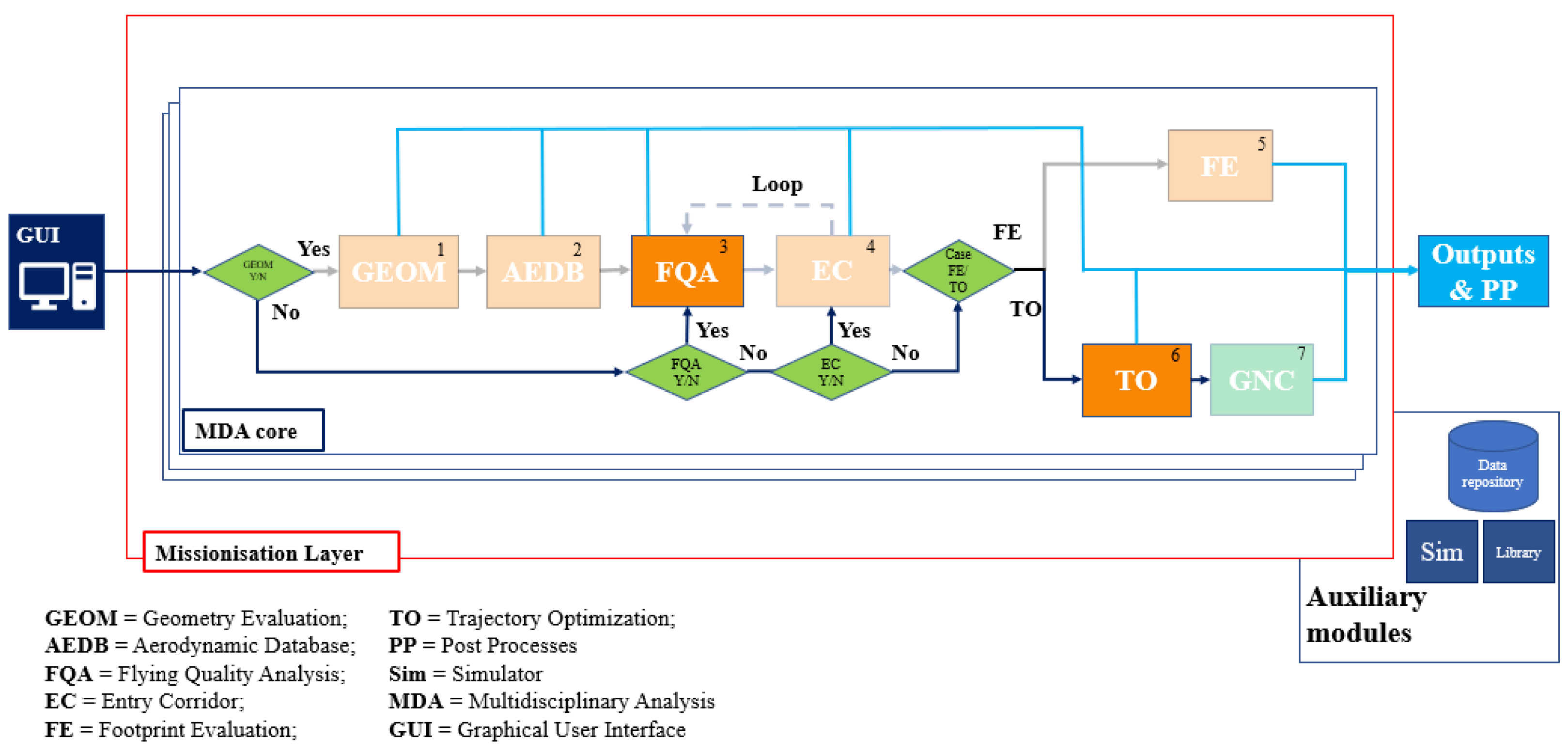
For the case analysed in this paper, the disciplines used are only the FQA and the TO building blocks. The geometry and the aerodynamic database of the vehicle are fixed and are provided as input. Moreover, the aerothermal mechanical constraints are imposed directly in the optimisation problem (
Section 4.1). The FQA is used only one time to obtain the trimmed AEDB, while the TO is called multiple time with different MECO conditions. In this case, the GNC is not considered, however the output of the TO tool can be easily used to initialise a GNC strategy, such as the one reported in [
11]. Furthermore, the Missionisation Layer is employed for the creation of the performance maps.
Figure 2 shows the high-level architecture of the tool with the active disciplines for study considered in this paper.
3. Mission Scenarios and System Models
This section briefly describes the RTLS and DRL mission phases. Then, it provides the equations of motion, the environment, and the vehicle models used to simulate the problem. Moreover, the section reports the longitudinal FQA analysis performed to trim the vehicle.
3.1. Mission Scenarios
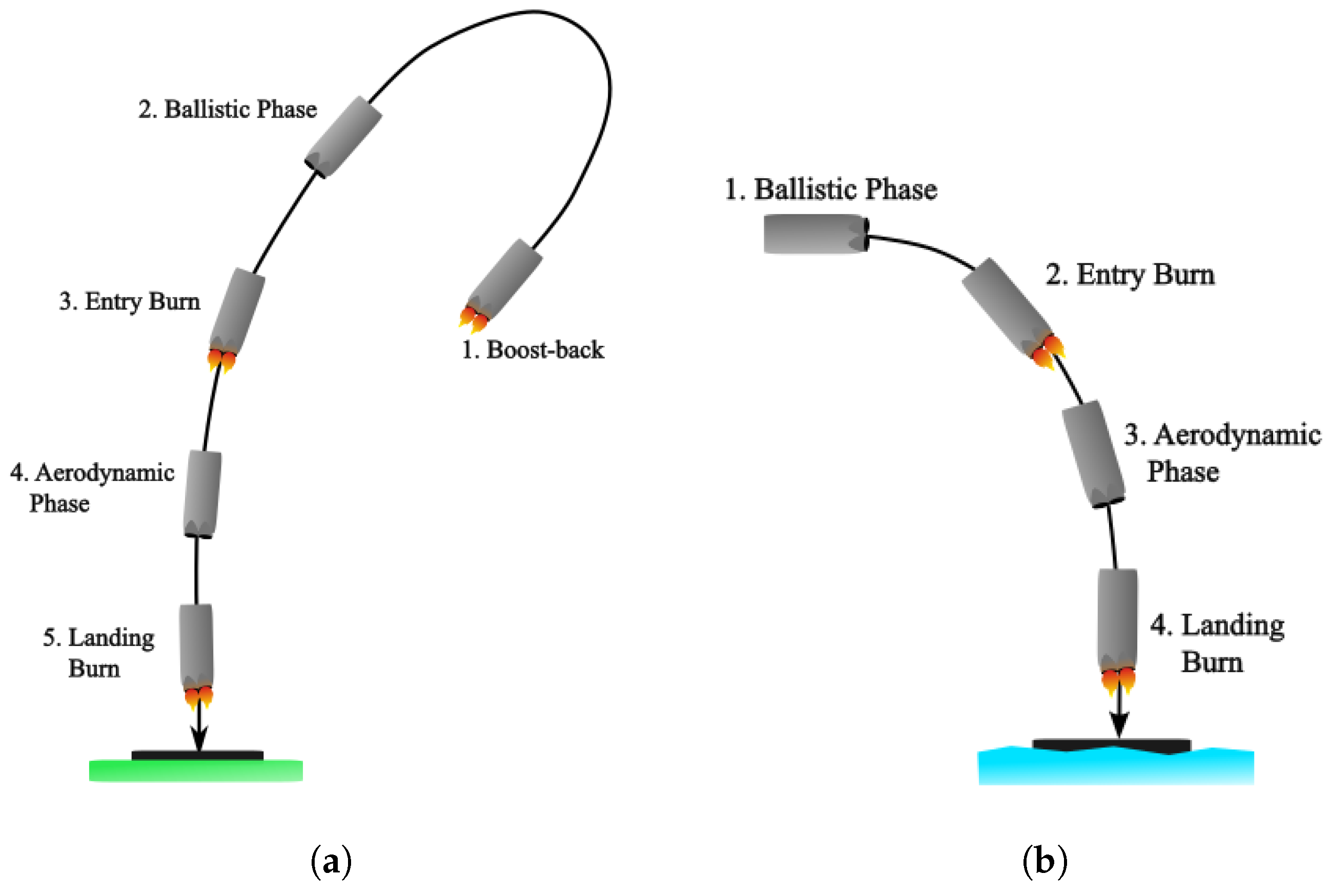
This paper considers two recovery scenarios characterized by vertical landing. The first one is the RTLS. In this case, the first stage of the space launcher returns towards the launch site or in its proximity, where it does a precise landing. It consists of five mission phases:
Boost-back: phase to achieve the inversion of the velocity and the targeting landing site;
Ballistic: phase in high-atmosphere in which the vehicle performs a ballistic flight;
Entry Burn: phase where the vehicle performs the entry burn to reduce the velocity while entering the denser atmosphere. This phase might not be necessary;
Aerodynamic phase: phase where the vehicle is controlled through aerodynamic control;
Landing Burn: phase in which the landing burn is performed to reduce the velocity till the pinpoint touchdown;
The DRL foresees the landing of the rocket first stage on a floating barge in the sea. It consists of four mission phases equal to the RTLS ones except for the boost-back [
4,
17].
Figure 3 shows the mission profiles for RTLS and DRL.
3.2. Dynamic Equations of Motion and Control
In this paper, the dynamics of the problem are formulated with point-mass 3DoF equations of motion expressed with Cartesian coordinates in Earth-Centered Earth-Fixed (ECEF) reference frame [
18]. The equations are described by Equation (
1):
where
T is the thrust accounting the ambient pressure penalty term when the nozzle is not adapted.
D and
L are the aerodynamic drag and lift forces, while the side force is not considered since a null side-slip angle is assumed along the trajectory.
is the control variable, and it defines the thrust orientation during the powered phases and the vehicle attitude during the unpowered phases. The model, indeed, assumes the thrust aligned with the main axis of the main axis of the rocket. The attitude is linked to the Angle-of-Attack (AoA) by
. It worth noting that the formulation of
has a minus sign such that during the descent the AoA is defined around 0
, and not 180
. The vector
is given by
, and it gives the direction of the lift.
is the specific impulse.
is the term relative to the acceleration due to the Earth rotation, and it is given by
, where
.
3.3. Environmental Models
The gravity assumes a spherical Earth with a standard gravitational parameter and a mean radius of 6378 km, i.e., . The rotation of the Earth is .
The atmosphere is modelled by using the US76 model without considering the winds [
19].
3.4. Vehicle Model: First Stage Features
The vehicle is a small-lift space launcher with similar size and performance to the Electron of RocketLab [
6]. Given the specific focus on the entry, descent, and landing phase, only the attributes of the first stage are considered. The stage body has a longitudinal length of 12 m and a base diameter of 1.2 m. The top of the first stage is equipped with planar fins designed to trim the vehicle during the aerodynamic phase of the trajectory. The fins have a mean aerodynamic chord of 0.5 m and, a wing span of 0.5 m. At the MECO, the first stage has a gross mass of 2000 kg and a dry mass of 950 kg. Approximately 10% of the propellant utilised during ascent is reserved for recovery purposes. Typically, small-lift launchers do not account additional propellant budget for a powered landing, that consequently affects the payload capability of the launchers with respect to its expendable version.
The vehicle has nine engines but it can only use three during the recovering manoeuvres and landing. Each engine is characterised by a specific impulse of 311 s, with a nominal thrust of 25 kN at sea level. The nozzles are adapted at an altitude of 8 km from the ground, and each of them has an exit area of 0.26 m
2. The thrust is modelled using the general rocket equations accounting the expansion losses due to the change in the atmospheric pressure with the altitude [
20].
3.5. Aerodynamic Model
The untrimmed aerodynamic database of the launch vehicle is obtained with DATCOM-like methods [
21] to model the variation of the drag coefficient
, the lift coefficient
, and the pitching moment coefficient
in the function of the Angle-of-Attack (AoA), the Mach number, and the deflection of the planar fins [
22]. The dataset is defined within a Mach number range of
, an AoA of
with the nozzle base plate directed against the flow, and the fins deflection included between
. The database is used to build three functions
,
, and
that are utilised for the FQA and for estimating the aerodynamic forces throughout the simulation. These functions linearly interpolate the obtained datasets. During the retro-propulsive manoeuvres, the effect of aerodynamic forces is reduced due to the interaction of the plume with the external flow, according to [
18,
23,
24,
25].
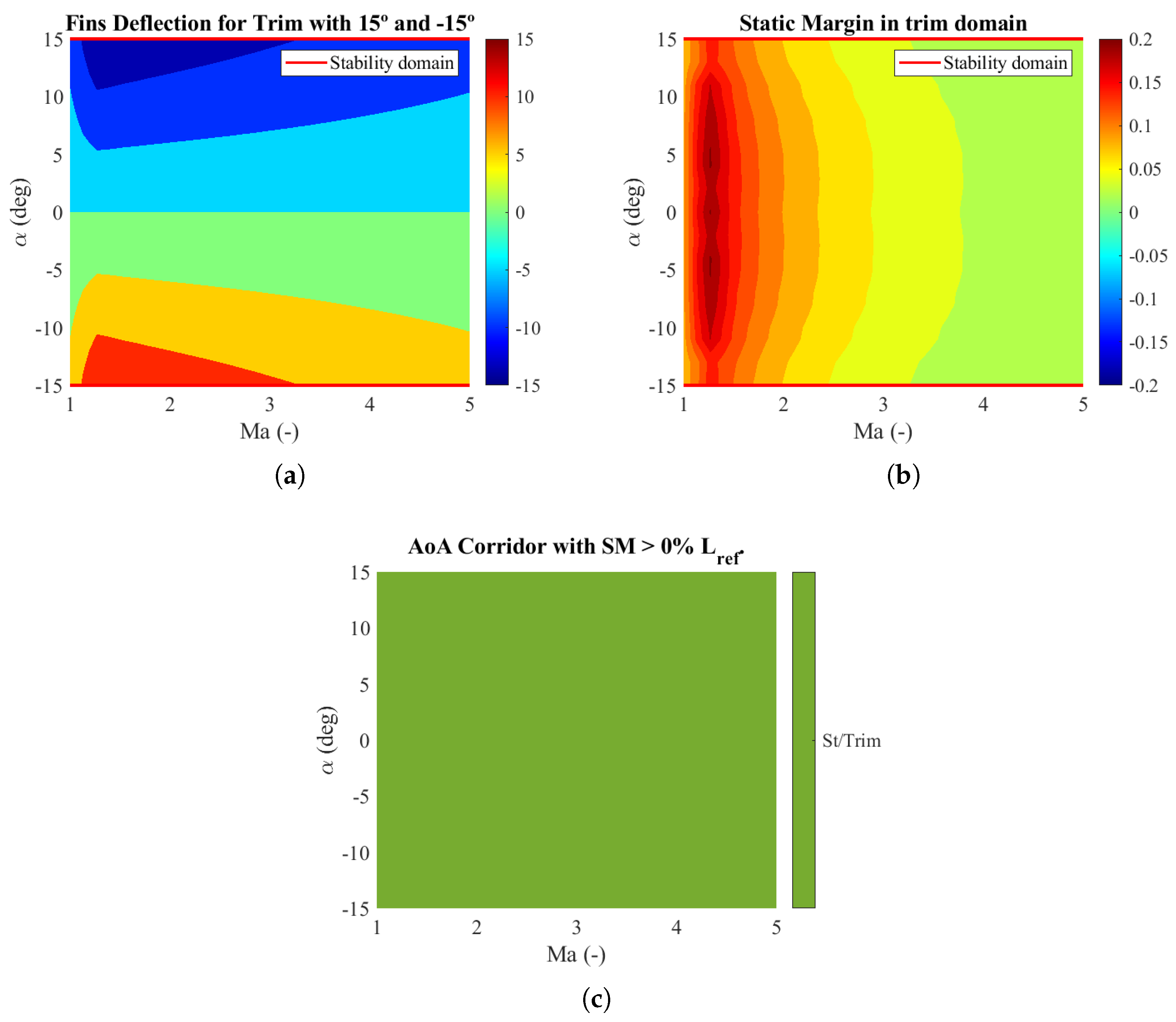
3.6. Flying Qualities Analysis
The aerodynamic model is analysed to determine its longitudinal trimmability and static stability. The objective of this analysis is to establish the feasibility of an AoA Entry Corridor during the aerodynamic phase of descent. In the context of this study, the AoA Entry Corridor delineates specific areas within the Mach-AoA plane where a stable and static trim solution can be identified, while accounting for various flight mechanics constraints. One such constraint involves the maximum allowable fins deflection, set at
[
4].
The trim condition is given when the torques acting on the vehicles are zero, and it obtained by computing the fins deflection
that results in a
, so when:
where, commonly, the
is given by [
26]:
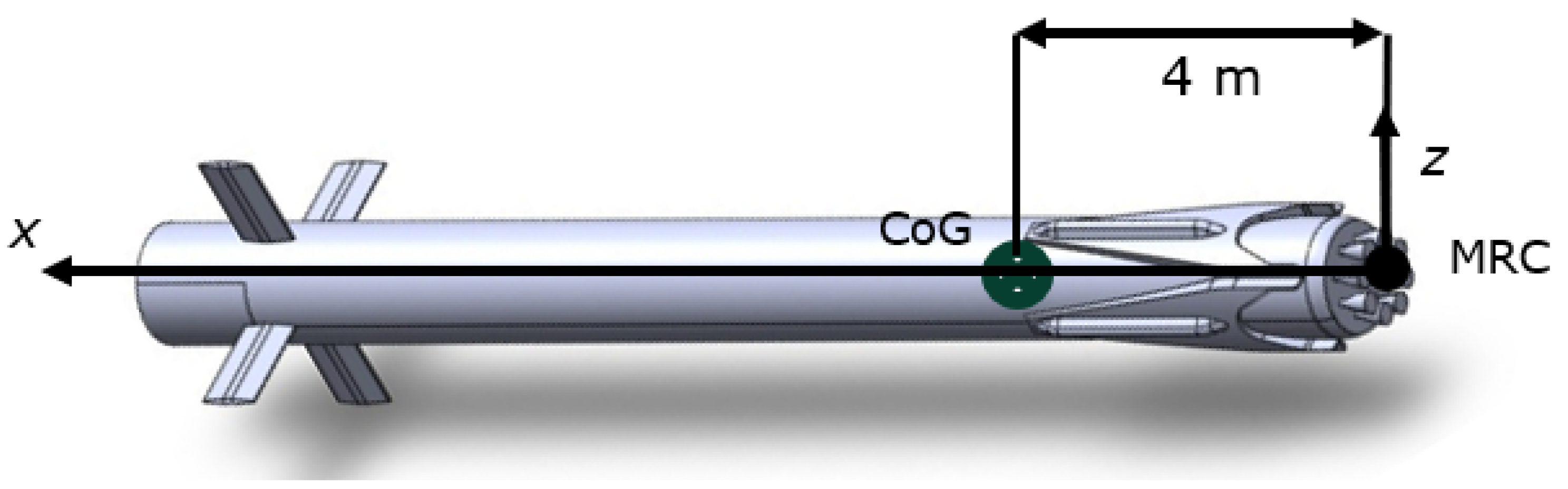
The additional torques are generated by the transport terms, due to the difference of the CoG position and the Moment Reference Center position:
The analysis is performed by considering a CoG location towards the engines, at 4 m from the nozzle base plate (
Figure 4). During the aerodynamic phase, indeed, the first stage is characterised by a low propellant load. The Moment Reference Center was placed at the nozzle base plate, which correspond to [0 0 0] m.
The static stability of the trim point is evaluated by means of the static margin [
28]:
where
defines the derivative of the considered aerodynamic coefficient with respect to the AoA. If the static margin is positive (as defined in Equation (
5)), the system is statically stable.
Figure 5 shows the result of the FQA. In particular,
Figure 5a,b outline the feasibility of a stable trim solution in the entire domain of interest. Thus, based on the models available, the planar fins can fully trim the rocket during the aerodynamic phase, and a feasible AoA entry corridor can be defined (green region
Figure 5c).
The results obtained with the FQA are used to achieve a trimmed aerodynamic database and exploited during the aerodynamic phase of the mission. Future work foresees the extension of this analysis during the landing burn manoeuvre, and a more complete FQA that also investigates the lateral and dynamical stability.
4. Optimisation Problem and Surrogate Model Formulation
Trajectory optimisation is a particular case of an optimal control problem. In this work, the trajectory optimisation problem is formulated in multiple phases and is solved with a local gradient-based algorithm. The problem is transformed into a Nonlinear Programming (NLP) problem with the direct Hermite-Simpson scheme transcription method [
29,
30]. Then, the NLP is solved by using a Sequential Quadratic Programming (SQP) algorithm available in MATLAB’s function
fmincon [
31,
32]. The optimisation variables are the state and control variables and a set of problem parameters, such as the final time of each phase.
The optimal control problem is solved by considering several MECO conditions. However, due to the relatively high computational time, a surrogate model is created to approximate the output of the problem from a predefined number of solutions obtained. Then, the performance maps are built by evaluating the metamodel in the domain of interest.
4.1. Multiphase Optimal Control Problem Formulation
In this paper, the propellant-optimal re-entry and landing problem is decomposed in user-defined phases for both the RTLS and DRL. The subdivision in phases allows for characterising the optimal control problem with different dynamics and path constraints, resulting in a better representation of the whole problem.
The RTLS multiphase optimal control problem is formulated in five phases, while the DRL is in four (
Section 3.1). The aim of the optimal control problem is to obtain the control vector
, the thrust magnitude
, and the final time of each phase
which maximise the final mass
, without violating a set of constraints. The control
u(
t) gives the direction of the thrust when the engine is switched on, otherwise, it simulates the attitude of the rocket. The state variable is given by
. The apexes
p and
k define the phase id: it is
for RTLS, and
for DRL.
P stands for the last phase of the mission, numbered 5 and 4, respectively for RTLS and DRL. The thrust magnitude is present only in phases 1, 3, 5 for RTLS, while 2 and 4 for DRL. In this work, the problem has been formulated such that the thrust throttling is bounded within the 49% and the 100% during the burning phases [
33].
Table 1 summarises the formulation of the optimisation problem both for RTLS and DRL, highlighting the constraints considered.
It is worth mentioning that for the DRL case, the final conditions are not imposed in the boundary conditions, while the cost function is augmented with penalty terms to ensure that the final altitude is equal to the Earth surface, and the final velocity reaches a desired value. In this way, the optimisation algorithm can select the best landing position on the Earth surface. This operation is done since the dynamics of the problem has been formulated in Cartesian coordinates. On the other hand, for the RTLS the final conditions are strictly imposed, since the landing site is prescribed.
As previously indicated, the final time for each phase is an optimisation parameter. Consequently, the optimisation procedure could identify a solution that omits a particular phase of the return mission. For instance, it might forego the entry burn maneuver if the ballistic and aerodynamic phases prove sufficient for decelerating the launch vehicle prior to executing the landing burn.
4.2. Surrogate Model
To cope with the relatively high computational time needed to solve the optimisation problem, a surrogate model is used to estimate the mission performance in the full domain of interest. In this work, Gaussian Radial Basis Functions (RBFs) are used to interpolate the solutions of a predefined set of sample points and build the surrogate model. In this work, the sample points are given by a set of computed optimal solutions. A general RBF metamodel can be formulated as (Equation (
6)):
where
N is the number of sample points;
is the radial function. In this case, the radial function is given by the Gaussian shape
.
are the weight coefficients, and
c is the shape parameter, which affects the conditioning of the problem [
14]. The coefficient vector
is calculated in this way (Equation (
7)):
In the study case presented in this paper, the output of the surrogate model is the mass of the first stage at the landing point, while the inputs are the MECO conditions. In this work, the ascent trajectory has not been designed, and reference values are used to define the MECO [
6].
5. Test Cases and Results
Within this section, the results of the analysis are presented. The examined scenarios consider the Guiana Space Center as the launch site. Consequently, this site serves as the designated landing location for the RTLS strategy, while, as introduced in
Section 4.1, the DRL does not account for a specific landing position.
Table 2 provides a comprehensive overview of the problem parameters, the values of the path constraints, and the final conditions taken into account during the optimisation. For building the performance maps, three key parameters are used to delineate the variation of the MECO conditions. In the context of the RTLS, the variables are the norm of the MECO velocity, the Flight-Path-Angle (FPA) at MECO, and the downrange distance between the MECO and the launch site, which is a function of the longitude at MECO [
34]. For the DRL, the variables are the altitude at MECO, the norm of the MECO velocity, and the FPA.
Table 2 also provides the fixed variables at MECO. These fixed parameters have been determined through preliminary dry runs to assess their impact on the final mass.
Table 3 outlines the variables at MECO and their respective ranges of variation.
In
Table 2 and
Table 3, the variables are presented in spherical coordinates, which facilitates their physical interpretation. Nevertheless, the conversion into Cartesian coordinates can be accomplished by leveraging the relationships detailed in [
35]. The values of the dispersion at MECO are defined from [
4,
5]. However, these ranges can be accordingly tuned depending on the specific case and through the design of the ascent phase.
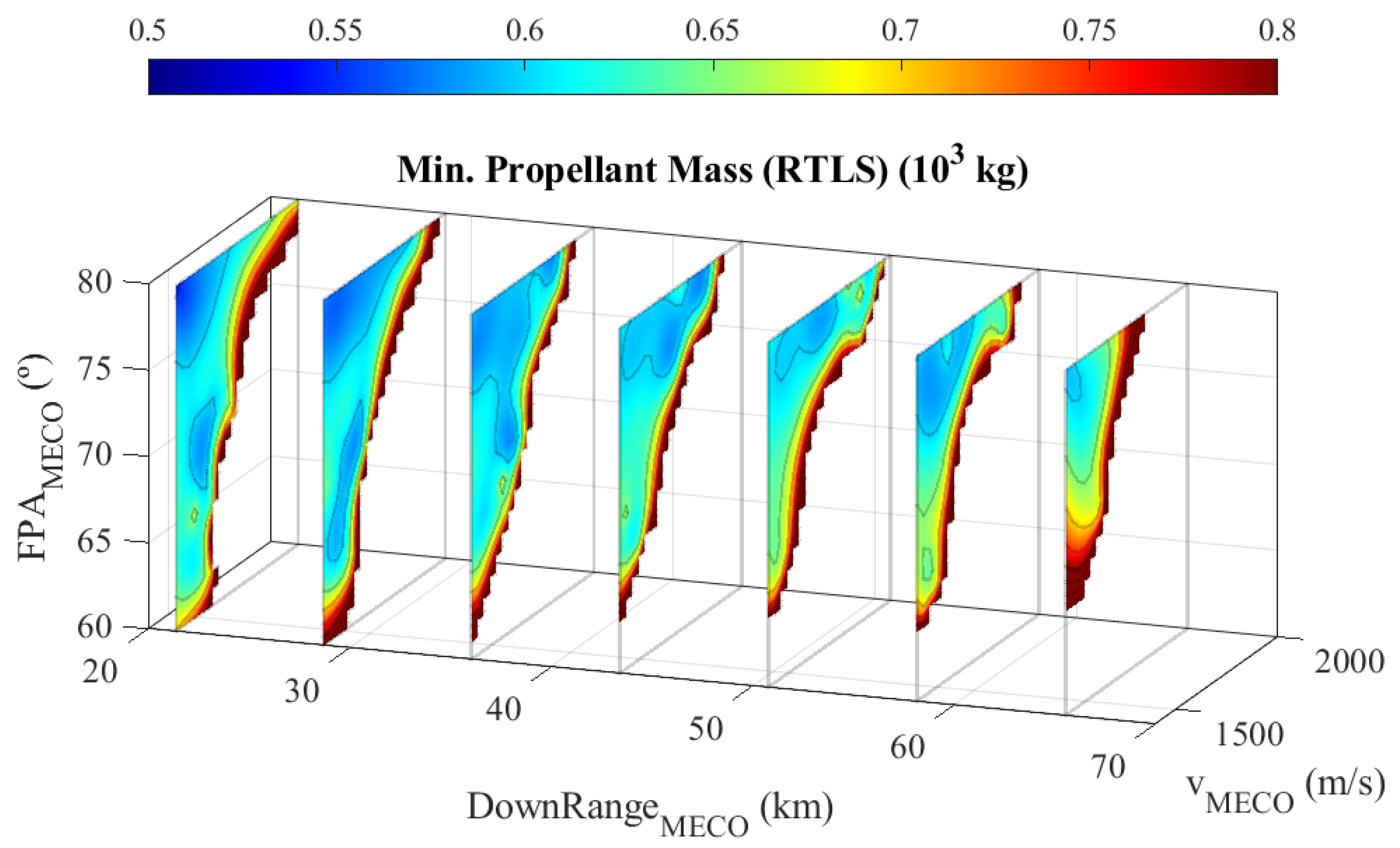
5.1. Return-to-Launch-Site
Figure 6 shows the map of the minimum propellant mass required to perform RTLS trajectories concerning the variations of the velocity norm, the FPA, and the downrange at MECO within the range reported in
Table 3. In this scenario, the remaining variables (altitude, latitude, and heading angle) are held constant, as indicated in
Table 2. In the case of RTLS, the metamodel is established by solving the optimisation problem across 123 sampled points (100 samples, 8 hypervertices, and 15 tests points). This operation is done in about 6 h in an Intel
® Core™ i7-8750H processor.
The results of the analysis convey that the required propellant mass follows the general pattern described below:
The necessary propellant mass increases with the growth of the downrange distance between the MECO and the launch site. This is anticipated as the engine has to operate for an extended duration to cover the greater distance during the boost-back maneuver.
The propellant mass decreases as the FPA increases. This phenomenon is attributed to the fact that less propellant is required to reverse the vehicle’s velocity when horizontal velocity is lower (associated with a high FPA) during the boost-back maneuver.
The required propellant mass increases as the magnitude of the velocity increases. This is because the system needs more propellant, both during the boost-back maneuver to reverse the speed and during the entry burn (if applicable) and landing burn to decelerate the vehicle.
Furthermore, the findings indicate that a RTLS approach is not feasible across the entire domain of interest. Under these specific MECO conditions, the propellant budget is not sufficient of achieving a trajectory that complies with both the aerothermal and mechanical load constraints, resulting in void regions. Additionally, it is noteworthy that the feasible region diminishes as the downrange distance increases. This observation underscores the pivotal role of this variable in securing a feasible and efficient RTLS trajectory.
Figure 7 presents the feasible trajectories achieved in two key domains: the altitude-velocity domain (
Figure 7a) and the altitude-downrange domain (
Figure 7b). These figures illustrate the diversity of solutions based on the MECO conditions. In
Figure 7a, the entry corridor is reported in order to show that all aerothermal-mechanical loads constraints are not violated. Moreover, it is apparent that in certain instances, the optimiser has identified a solution that involves only two burning maneuvers, thus bypassing the entry burn. This outcome deviates from the typical mission profile followed by the Falcon 9. Consequently, further analyses are foreseen for these specific cases in future investigations.
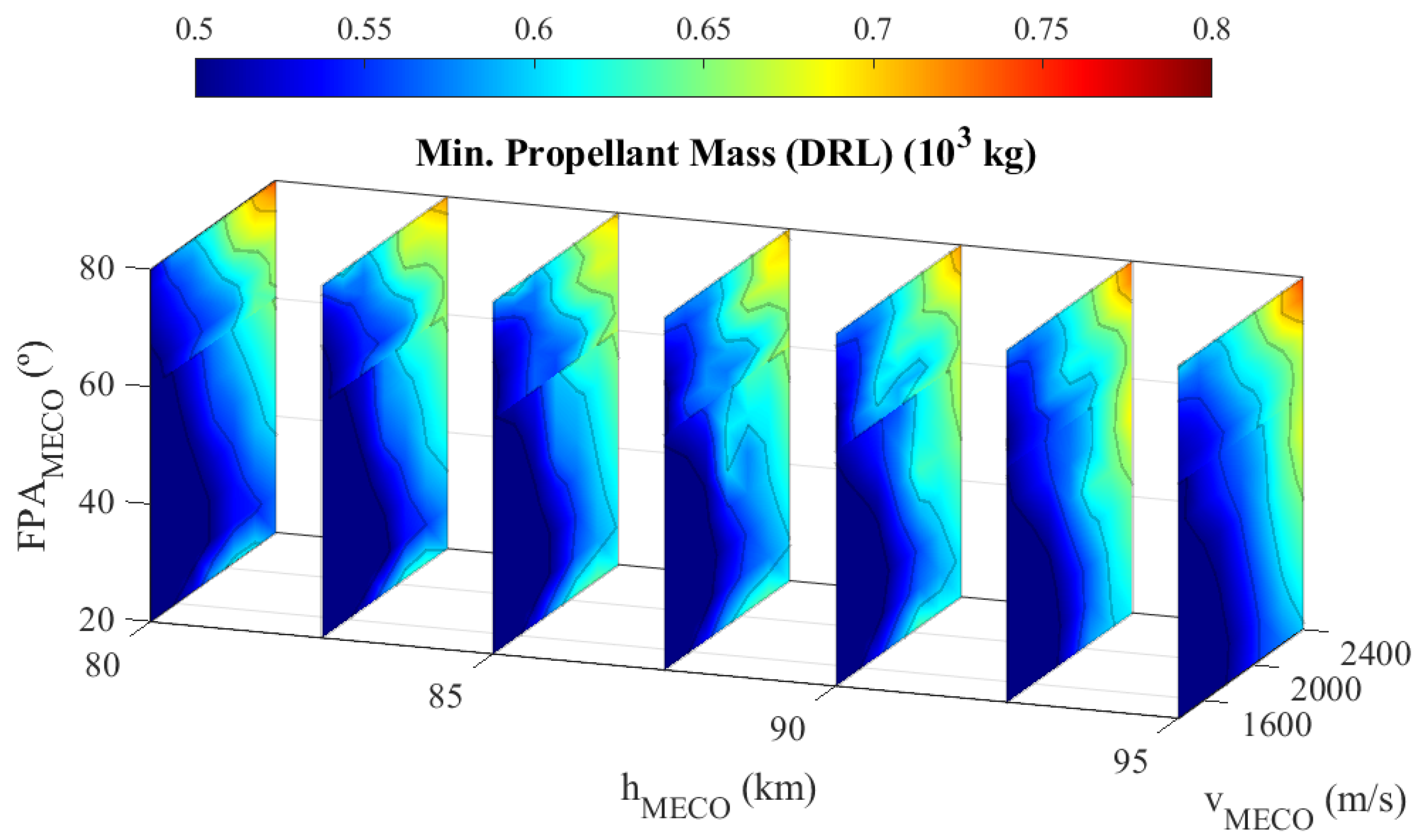
5.2. Downrange Landing
Figure 8 provides the performance map generated for the DRL strategy. In this context, the necessary propellant mass is determined based on the magnitude of the velocity, the Flight Path Angle (FPA), and the altitude at MECO, as outlined in
Table 3. The latitude, longitude, and heading angle remain fixed parameters for the DRL strategy, as indicated in
Table 2. To create the metamodel for this scenario, the optimisation problem is solved at 250 distinct points (200 samples, 16 hypervetices and 34 test points). This operation is done in about 5 h in the same processor. Here, the computational time is lower because the convergence for the DRL is faster, since the trajectory has a smoother shape and the recovery is feasible in the entire domain of interest. The initial population of MECO conditions have been generated with Latin Hypercube Sampling method. In this case, the domain has been split into two parts being larger.
Similar to the RTLS scenario, the analysis results for the DRL strategy exhibit the following common trends:
The propellant consumption rises as the FPA increases, particularly at higher velocities. This trend arises from the fact that a higher FPA at MECO results in a steeper descent trajectory, necessitating longer retro-propulsive maneuvers to mitigate aerothermal and mechanical loads and to decelerate the rocket. Conversely, a shallower FPA leads to smoother trajectories with reduced loads.
An increase in the velocity at MECO is correlated with an augmented requirement for propellant mass, as longer burns are essential to decelerate the launch vehicle, reduce aerothermal and mechanical loads, and achieve the desired touchdown conditions.
The altitude at MECO does not exert a significant impact on propellant consumption.
The findings indicate that the DRL strategy is feasible within the complete range of interest for the case under examination. This implies that for each MECO condition falling within the range specified in
Table 3, a return trajectory can be defined that satisfies the propellant budget, meets the limits on aerothermal and mechanical loads, and fulfills the touchdown conditions.
Also in this case,
Figure 9 displays the attainable trajectories in both the altitude-velocity domain (
Figure 9a) and the altitude-downrange domain (
Figure 9b). These figures illustrate the diversity of solutions based on varying MECO conditions. Moreover, the entry corridor in
Figure 9a highlights that all aerothermal-mechanical loads constraints are respected.
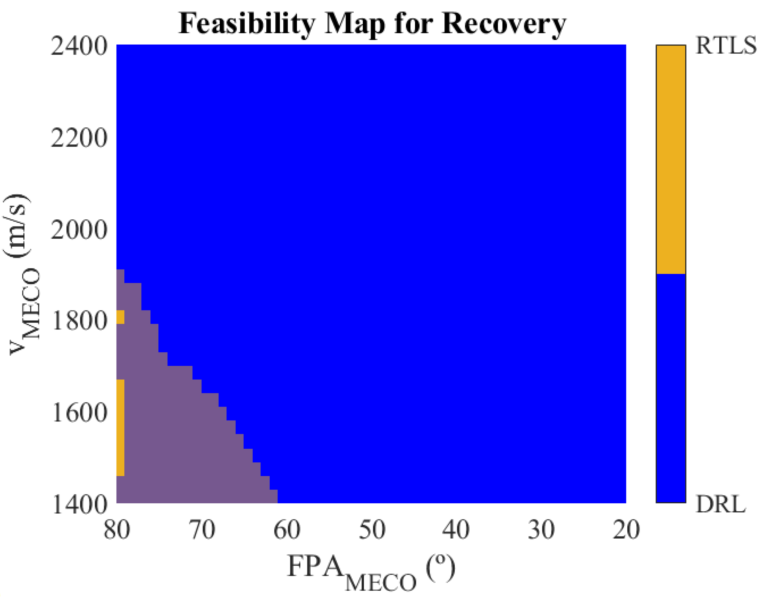
5.3. Recovery Feasibility Region Analysis
Based on the outcomes presented in
Section 5.1 and
Section 5.2, an overall feasibility region is established, taking into account both the RTLS and DRL recovery strategies, particularly concerning the velocity and FPA conditions at MECO. To delineate this feasibility region, data from the performance maps obtained in the previous sections is considered. For RTLS, a downrange distance between MECO and the landing site of approximately 35 km is taken into account, while for DRL, an altitude at MECO of 85 km is considered.
Figure 10 provides a comprehensive view of the recovery feasibility map for the analywed launch vehicle, covering the range of MECO velocity and FPA explored in this mission feasibility analysis. This single plot allows for a direct comparison of which recovery strategy is feasible under specific MECO conditions and also emphasises which strategy is more efficient in terms of propellant consumption.
Specifically, in this instance,
Figure 10 highlights areas in yellow where RTLS is both feasible and more efficient than DRL. In blue, it showcases regions where DRL is feasible and more efficient than RTLS. The intersected violet area denotes the region in which both strategies are feasible, but DRL overtakes RTLS in terms of efficiency.
This analysis shows that DRL is more flexible and efficient than RTLS in terms of the required propellant mass alone. However, it is important to note that when considering a broader spectrum of parameters, such as refurbishment, barge operations, and transportation time and costs, the analysis could yield different results. Furthermore, it is noteworthy that in several RTLS cases, the optimiser identifies solutions involving just two burns (boost-back and landing burn). These specific solutions, which consume a comparable amount of propellant to DRL solutions, are particularly interesting and further investigation can be done in future research, since the RTLS has lower operational cost than DRL [
36].
The feasibility region analysis can be used as a valuable tool throughout the missionisation process. It can be leveraged to make informed decisions when selecting the most efficient recovery strategy based on mission requirements and objectives. These objectives, including the target orbit and payload mass, can be translated into specific MECO conditions. By utilising the feasibility region analysis, mission planners and designers can make strategic choices that align with the project’s goals and performance targets.
The feasibility map may be used as a general missionisation tool which gives information with respect to system aspect and not only mission parameters. For example, it could be interesting how the maps evolves if the rocket is characterised by an higher drag coefficient and a larger thrust-to-weight ratio. In this case, for instance, the feasibility region relative to the RTLS is expected to grow, since less propellant is needed to slow down the vehicle. Moreover, the approach may directly consider the mass ratio and the V budget of the launcher in order to also compare different category of launch vehicles from system options.
6. Conclusions
The paper presents a comprehensive study of mission performance with a focus on propellant mass across a wide range of MECO conditions for a VL-RLV. This study considers both the RTLS and DRL recovery strategies. Additionally, a feasibility region has been determined to facilitate the comparison of these two recovery approaches.
The paper outlines the methodology used to model the propellant-optimal return trajectory for a VL-RLV and explains the process employed to generate performance maps. The results highlight how different MECO conditions impact the consumed propellant mass, while accounting for propellant budget, aerothermal, and mechanical load constraints, especially in the context of a small-lift launch vehicle. Overall, the findings suggest that DRL represents a more versatile and efficient solution when considering performance and the parameters under investigation. Furthermore, this approach can be extended by conducting a parametric analysis of a launcher’s characteristics based on its mass ratio and V budget. This expands its applicability beyond specific launch vehicles, making it applicable to a broad spectrum of vehicles with similar engine efficiency ratios. This extension may offer valuable insights for sizing and evaluating various system options for trade-offs.
Future upgrades may foresee the inclusion of a more detailed model of the vehicle AEDB, as well as, other improvements regarding the dynamic and environment models, such as the assessment of the solutions with a 6DoF simulator. Moreover, different sources of dispersion and uncertainties may be analysed.
These results can be included in the mission analysis and GNC missionisation process for any reusable space launch vehicle.
Author Contributions
J.G. Definition and implementation of the tool, and carrying out the analysis. J.G. and G.D.Z. definition of the methodology and application case. J.G. writing. G.D.Z. and M.L. supervision, review and editing. All authors have read and agreed to the published version of the manuscript.
Funding
The project leading to this application has received funding from the European Union’s Horizon 2020 research and innovation program under the Marie Skłodowska-Curie grant agreement No. 860956.
Institutional Review Board Statement
Not applicable.
Informed Consent Statement
Not applicable.
Data Availability Statement
Data are not available due to privacy restrictions.
Acknowledgments
Thank to Federico Toso, Giuseppe Guidotti, and Atmospheric Flight competence center team for the support.
Conflicts of Interest
The authors declare no conflict of interest.
References
- Patureau de Mirand, A.; Bahu, J.M.; Gogdet, O. Ariane Next, a vision for the next generation of Ariane Launchers. Acta Astronaut. 2020, 170, 735–749. [Google Scholar] [CrossRef]
- Simplício, P.; Marcos, A.; Bennani, S. Guidance of Reusable Launchers: Improving Descent and Landing Performance. J. Guid. Control. Dyn. 2019, 42, 2206–2219. [Google Scholar] [CrossRef]
- Sagliano, M.; Heidecker, A.; Hernández, J.M.; Farì, S.; Schlotterer, M.; Woicke, S.; Seelbinder, D.; Dumont, E. Onboard Guidance for Reusable Rockets: Aerodynamic Descent and Powered Landing. In Proceedings of the AIAA Scitech 2021 Forum, Virtual, 11–15 & 19–21 January 2021. [Google Scholar] [CrossRef]
- De Zaiacomo, G.; Arnao, G.; Bunt, R.; Bonetti, D. Mission engineering for the RETALT VTVL launcher. CEAS Space J. 2022, 14, 533–549. [Google Scholar] [CrossRef]
- Falcon 9 Stage 1 Landing Analysis. 2017. Available online: https://www.reddit.com/ (accessed on 6 November 2023).
- Electron. 2023. Available online: rocketlabusa.com (accessed on 6 November 2023).
- Vila, J.; Hassin, J. Technology acceleration process for the THEMIS low cost and reusable prototype. In Proceedings of the 8th European Conference for Aeronautics and Space Sciences, Madrid, Spain, 1–4 July 2019. [Google Scholar]
- CNES. CALLISTO: Testing the Concept of a Reusable Launcher First Stage.
- Kulu, E. Small Launchers—2021 Industry Survey and Market Analysis. In Proceedings of the 72nd International Astronautical Congress (IAC 2021), Dubai, United Arab Emirates, 25–29 October 2021. [Google Scholar]
- Guadagnini, J.; Zaiacomo, G.D. Multidisciplinary Modeling for Missionisation of Re-entry Vehicles. In Proceedings of the AIAA SCITECH 2023 Forum, National Harbor, MD, USA, 23–27 January 2023. [Google Scholar] [CrossRef]
- Guadagnini, J.; Lavagna, M.; Rosa, P. Model predictive control for reusable space launcher guidance improvement. Acta Astronaut. 2022, 193, 767–778. [Google Scholar] [CrossRef]
- You, S.; Wan, C.; Dai, R.; Rea, J.R. Learning-Based Onboard Guidance for Fuel-Optimal Powered Descent. J. Guid. Control. Dyn. 2021, 44, 601–613. [Google Scholar] [CrossRef]
- Sagliano, M.; Mooij, E.; Theil, S. Onboard Trajectory Generation for Entry Vehicles via Adaptive Multivariate Pseudospectral Interpolation. J. Guid. Control. Dyn. 2017, 40, 466–476. [Google Scholar] [CrossRef]
- Shi, R.; Long, T.; Ye, N.; Wu, Y.; Wei, Z.; Liu, Z. Metamodel-based multidisciplinary design optimization methods for aerospace system. Astrodynamics 2021, 5, 185–215. [Google Scholar] [CrossRef]
- Harloff, G.; Berkowitz, B. HASA: Hypersonic Aerospace Sizing Analysis for the Preliminary Design of Aerospace Vehicles; NASA Lewis Research Center Group: Cleveland, OH, USA, 1988.
- Saraf, A.; Leavitt, J.; Ferch, M.; Mease, K. Landing footprint computation for entry vehicles. In Proceedings of the AIAA Guidance, Navigation, and Control Conference and Exhibit, Providence, RI, USA, 16–19 August 2004; p. 4774. [Google Scholar]
- Simplício, P.; Marcos, A.; Bennani, S. A Reusable Launcher Benchmark with Advanced Recovery Guidance. In Proceedings of the 5th CEAS Conference on Guidance, Navigation & Control, Milan, Italy, 3–5 April 2019. [Google Scholar]
- Brendel, E.; Hérissé, B.; Bourgeois, E. Optimal guidance for toss back concepts of reusable launch vehicles. In Proceedings of the 8th European Conference for Aeronautics and Space Sciences, Madrid, Spain, 1–4 July 2019. [Google Scholar]
- National Oceanic and Atmospheric Administration. U.S. Standard Atmosphere, 1976; United States Air Force; National Oceanic and Atmospheric Administration: Washington, DC, USA, 1976.
- Rocket Thrust Equation. 2021. Available online: https://www.grc.nasa.gov/www/k-12/airplane/rockth.html (accessed on 6 November 2023).
- Public Domain Aeronautical Software. References for the Digital Datcom Program. Available online: https://www.pdas.com/datcomrefs.html (accessed on 6 November 2023).
- Guadagnini, J.; De Zaiacomo, G.; Bussler, L. Aerodynamic Coefficients Estimation Tool for re-entry Vehicle Missionisation. In Proceedings of the 2nd International Conference on Flight Vehicles Aerothermodynamics and Re-entry Missions and Engineering (FAR), Heilbronn, Germany, 19–23 June 2022. [Google Scholar]
- Laureti, M.; Karl, S.; Marwege, A.; Guelhan, A. Aerothermal Databases and CFD Based Load Predictions. In Proceedings of the 2nd International Conference on Flight Vehicles Aerothermodynamics and Re-entry Missions and Engineering (FAR), Heilbronn, Germany, 19–23 June 2022. [Google Scholar] [CrossRef]
- Marwege, A.; Hantz, C.; Kirchheck, D.; Klevanski, J.; Vos, J.; Laureti, M.; Karl, S.; Guelhan, A. Aerodynamic Phenomena of Retro Propulsion Descent and Landing Configurations. In Proceedings of the 2nd International Conference on Flight Vehicles Aerothermodynamics and Re-entry Missions and Engineering (FAR), Heilbronn, Germany, 19–23 June 2022. [Google Scholar] [CrossRef]
- Vos, J.; Charbonnier, D.; Marwege, A.; Guelhan, A.; Laureti, M.; Karl, S. Aerodynamic investigations of a Vertical Landing Launcher configuration by means of Computational Fluid Dynamics and Wind Tunnel Tests. In Proceedings of the AIAA SCITECH 2022 Forum, San Diego, CA, USA, 3–7 January 2022. [Google Scholar] [CrossRef]
- Hirschel, E.H.; Weiland, C. Selected Aerothermodynamic Design Problems of Hypersonic Flight Vehicles; Springer Science & Business Media: Berlin/Heidelberg, Germany, 2009; Volume 229. [Google Scholar]
- RETALT-Retro Propulsion Assisted Landing Technologies. 2023. Available online: https://www.retalt.eu/ (accessed on 6 November 2023).
- Haya Ramos, R.; Penin, L.; Parigini, C.; Kerr, M.; Preaud, J.P.; Ganet, M.; Bennani, S.; Martinez Barrio, A. Flying Qualities Analysis for Re-entry Vehicles: Methodology and Application. In Proceedings of the AIAA Guidance, Navigation, and Control Conference, Portland, OR, USA, 8–11 August 2011. [Google Scholar] [CrossRef]
- Betts, J.T. Practical Methods for Optimal Control and Estimation Using Nonlinear Programming; Society for Industrial and Applied Mathematics (SIAM). 2010. Available online: https://epubs.siam.org/doi/abs/10.1137/1.9780898718577 (accessed on 6 November 2023).
- Topputo, F.; Zhang, C. Survey of Direct Transcription for Low-Thrust Space Trajectory Optimization with Applications. Abstr. Appl. Anal. 2014, 2014, 851720. [Google Scholar] [CrossRef]
- Boggs, P.; Tolle, J. Sequential Quadratic Programming. Acta Numer. 1995, 4, 1–51. [Google Scholar] [CrossRef]
- Murray, W. Sequential quadratic programming methods for large-scale problems. Comput. Optim. Appl. 1997, 7, 127–142. [Google Scholar] [CrossRef]
- Spada, F.; Ghignoni, P.; Botelho, A.; De Zaiacomo, G.; Rosa, P. Successive Convexification-based fuel optimal high altitude guidance of the Retalt reusable launcher. In Proceedings of the ESA GNC-ICATT, Sopot, Poland, 12–16 June 2023. [Google Scholar]
- Liu, X.; Shen, Z.; Lu, P. Solving the maximum-crossrange problem via successive second-order cone programming with a line search. Aerosp. Sci. Technol. 2015, 47, 10–20. [Google Scholar] [CrossRef]
- Mooij, E. The Motion of a Vehicle in a Planetary Atmosphere; Report LR-768; Delft University of Technology, Faculty of Aerospace Engineering: Delft, The Netherlands, 1994. [Google Scholar]
- Stappert, S.; Wilken, J.; Bussler, L.; Sippel, M. A Systematic Comparison of Reusable First Stage Return Options. In Proceedings of the 8th European Conference for Aeronautics and Space Sciences, Madrid, Spain, 1–4 July 2019. [Google Scholar]
| Disclaimer/Publisher’s Note: The statements, opinions and data contained in all publications are solely those of the individual author(s) and contributor(s) and not of MDPI and/or the editor(s). MDPI and/or the editor(s) disclaim responsibility for any injury to people or property resulting from any ideas, methods, instructions or products referred to in the content. |
© 2023 by the authors. Licensee MDPI, Basel, Switzerland. This article is an open access article distributed under the terms and conditions of the Creative Commons Attribution (CC BY) license (https://creativecommons.org/licenses/by/4.0/).


