${\mathcal{L}}_1$ Adaptive Control Based on Dynamic Inversion for Morphing Aircraft

Abstract

Morphing aircraft are able to keep optimal performance in diverse flight conditions. However, the change in geometry always leads to challenges in the design of flight controllers. In this paper, a new method for designing a flight controller for variable-sweep morphing aircraft is presented—dynamic inversion combined with ${\mathcal{L}}_1$ adaptive control. Firstly, the dynamics of the vehicle is analyzed and a six degrees of freedom (6DOF) nonlinear dynamics model based on multibody dynamics theory is established. Secondly, nonlinear dynamic inversion (NDI) and incremental nonlinear dynamic inversion (INDI) are then employed to realize decoupling control. Thirdly, linear quadratic regulator (LQR) technique and ${\mathcal{L}}_1$ adaptive control are adopted to design the adaptive controller in order to improve robustness to uncertainties and ensure the control accuracy. Finally, extensive simulation experiments are performed, wherein the demonstrated results indicate that the proposed method overcomes the drawbacks of conventional methods and realizes an improvement in control performance.

1. Introduction

Morphing aircraft are flight vehicles that change their surface geometry to adapt to a range of flight conditions and provide mission flexibility and versatility [1,2]. Compared to conventional fixed-shape aircraft, morphing aircraft are able to provide more benefits and play a very important role in military and civil aviation as the future advanced aircraft. Recent years have seen increased research attention being given to morphing aircraft owing to their capability to diminish the compromises required in multiple flight conditions [3,4].

Nevertheless, morphing solutions lead to large changes in geometrical parameters and aerodynamic parameters, which also generate additional forces and moments during the morphing phase. Such increasing system uncertainty and complexity of the system significantly [5] and makes it more difficult to maintain stable flight. These problems have to be solved in order to get better performance throughout a flight. Therefore, it is of considerable significance to design a high-performance flight control system for morphing aircraft.

Currently, a large number of studies have been dedicated to developing a flight controller for morphing aircraft. Considering that an aircraft is a typical time-varying nonlinear system, many early researchers assumed that the vehicle dynamics could be described by a linear parameter varying (LPV) model. This approach simplifies and transforms the nonlinear dynamics model to an LPV model by using Jacobian linearization, and then many well-established linear control methods can be used [5]. Wang et al. proposed a robust LPV controller using velocity-based linearization [6], which lifted the restriction on the equilibrium point in the traditional method. Lu et al. utilized multiple parameter-dependent Lyapunov functions (MPDLFs) to design a switching LPV controller [7]. However, parameter uncertainties existing in the controller always have an impact on control performance. Cheng et al. designed a non-fragile switched LPV $H\infty$ controller to eliminate the negative effects caused by uncertainties and to ensure stability under the asynchronous switching phenomenon [8]. Yue et al. proposed a gain self-scheduled $H\infty$ controller, whose gains are adjusted automatically as a function of time and operating conditions to guarantee flight stability and performance [4]. And in [9], a controller based on MPDLFs with low computational complexity was presented, and the control matrix of the LPV system was not limited to being constant. But in the linear control methods mentioned above, the nonlinear dynamics system was approximated by a linear model. The process of linear approximation ignored the higher-order nonlinear terms and this would never represent the true behavior completely and accurately. Considering that a morphing aircraft in flight is a very complicated dynamic system, the loss of some important nonlinear characteristics would seriously affect the control performance [10].

Therefore, more and more researchers have employed nonlinear control methods to control morphing aircraft in recent years. Chen et al. transformed the nonlinear dynamics equations of the vehicle into an affine nonlinear form, and then a backstepping method was applied to design the controller [11]. Yuan et al. presented an adaptive controller designed by backstepping and based on the ${\mathcal{L}}_2$ gain [12]. In [13,14], an adaptive backstepping controller has been proposed, in which a radial basis function (RBF) neural network was used to estimate the uncertain terms of the aircraft. However, backstepping can involve intricate mathematics caused by the differentiation of nonlinear functions and requires a deep understanding of nonlinear system dynamics. The recursive structure that backstepping relies on can lead to cascading errors or the amplification of uncertainties. Even with the addition of a neural network, the uncertain nonlinearity of the vehicle cannot be accurately approximated, which limits the practical application of this method.

NDI is a well-known flight control technique with advantages of precise decoupling and quick response without the need for complicated gain scheduling over a wide flight envelope [15], which transforms the nonlinear system dynamics into a set of linear equations without ignoring any higher-order nonlinear terms. However, an NDI-based controller is extremely model-dependent, and subtle uncertainties such as unmodeled dynamics and external disturbances can reduce the robustness of the controller. Therefore, numerous extensions to NDI have been proposed to overcome these limitations and enhance the control performance. INDI is a variation on NDI, which retains the high-performance advantages of the latter while decreasing the dependency on the model and enhancing the robustness to model uncertainties [16]. Besides INDI, adaptive control is a control approach that aims to automatically adjust the control parameters in real-time based on the system’s dynamic behavior or changes in operating conditions to adapt to changes in system dynamics, parameter variations, and external disturbances. Xu et al. adopted NDI and INDI to design a basic flight controller of morphing aircraft [2]. Zhou et al. presented an incremental filtered nonlinear control method considering actuator dynamic compensation [17] and Li et al. presented an angular acceleration control method based on INDI and adaptive control [18].

On the one hand, many researchers have simplified the 6DOF nonlinear vehicle model into three degrees of freedom (3DOF), which limited the practical application of the proposed control methods. On the other hand, for some conventional nonlinear control methods, the design process of the controller is cumbersome, especially when the model complexity is increasing. In addition, model uncertainties and measurement errors may also seriously affect the control accuracy [19]. Compared to other control methods, adaptive control is relatively model-free and its addition can compensate for the effects of possible faults or unexpected uncertainties and achieve a substantial improvement in performance; however, it is difficult for conventional adaptive control methods to achieve the trade-off between control performance and robustness [20,21,22]. ${\mathcal{L}}_1$ adaptive control, an improvement of model reference adaptive control (MRAC) presented by Cao and Hovakimyan, appears to be beneficial both for robustness and performance [22,23,24], resolving the trade-off between the two by selecting a low-level filtering structure. By decoupling adaptation from robustness via continuous feedback, this control architecture enables fast adaptation with guaranteed robustness [22].

In this paper, a practical approach to the design of the flight controller of a variable-sweep morphing aircraft has been proposed. Firstly, the vehicle dynamics model with 6DOF has been established, in which the variables of the system were divided into different sets by the time-scale separation principle and the mathematical expressions were described in a state-space form. Secondly, INDI and NDI have been employed to design the basic controller to achieve the decoupling control of attitude angles $\alpha$, $\beta$, and $\mu$. Then, LQR and ${\mathcal{L}}_1$ adaptive control have been adopted to design the adaptive controller in order to enhance the control performance. Thirdly, a series of simulations have been conducted in the pre-designed scenarios. The results indicate the superiority of the proposed method. It is proved that the approach presented in this paper has realized an improvement in control performance and overcomes the drawbacks of conventional methods. The main contributions of our work are summarized as follows:

• Many other researchers focus on the 3DOF vehicle dynamics model, which is simply based on the longitudinal dynamics that generates pitching and forward motion. Different from them, we establish a 6DOF dynamics model which can fully describe the dynamic characteristics of the vehicle. This expands the application scope of our method.
• Compared to the traditional LPV-based morphing aircraft controller, we adopt a nonlinear control method to realize the design of our flight controller, which improves the control precision. The combination of dynamic inverse and ${\mathcal{L}}_1$ adaptive control provides a balance between control performance and robustness.
• Different from many other works that only adopt NDI to design the basic controller, we use NDI and INDI, respectively, to design it. In addition, the ${\mathcal{L}}_1$ adaptive controller we proposed aims at the error dynamics system instead of the vehicle system itself, which is distinct from nearly all other works adopting this method and can ensure the desired command tracking to the maximum extent.

The rest of this paper is structured as follows: Section 2 establishes the 6DOF nonlinear dynamics model of our morphing aircraft. Section 3 and Section 4 introduce the design of the dynamic inversion controller and the adaptive controller, respectively. Section 5 gives the stability analysis of our controller. In Section 6, simulations are performed and results presented. Finally, Section 7 concludes this paper.

2. Model Description

In this paper, BQM-34 Firebee UAV designed by NextGen Aviation is chosen as the baseline aircraft. Configuration variants were constructed in [25,26] to enable a better aerodynamic performance and accommodate various mission requirements, in which sweep angle $\Lambda$ ranges from ${15.97}^{\circ }$ to ${60}^{\circ }$. Some configuration specifications are provided in Table 1.

Table 1. Parameters of two different configurations.

Parameters	Loitor Configuration ($\mathbf{\Lambda }$ = ${15.97}^{\circ }$)	Dash Configuration ($\mathbf{\Lambda }$ = ${60}^{\circ }$)
Gross weight, m	907 kg
Wing weight, $m_w$	60 kg
Length	6.68 m
Wing span, b	6.802 m	3.842 m
Wing area, $S_{ref}$	4.5 m	5.765 m
Mean aerodynamic chord, $\overline{c}$	0.688 m	1.935 m
Aspect ratio	10.281	2.561
sweep angle $\Lambda$	${15.97}^{\circ }$	${60}^{\circ }$

2.1. Equations of Force and Moment

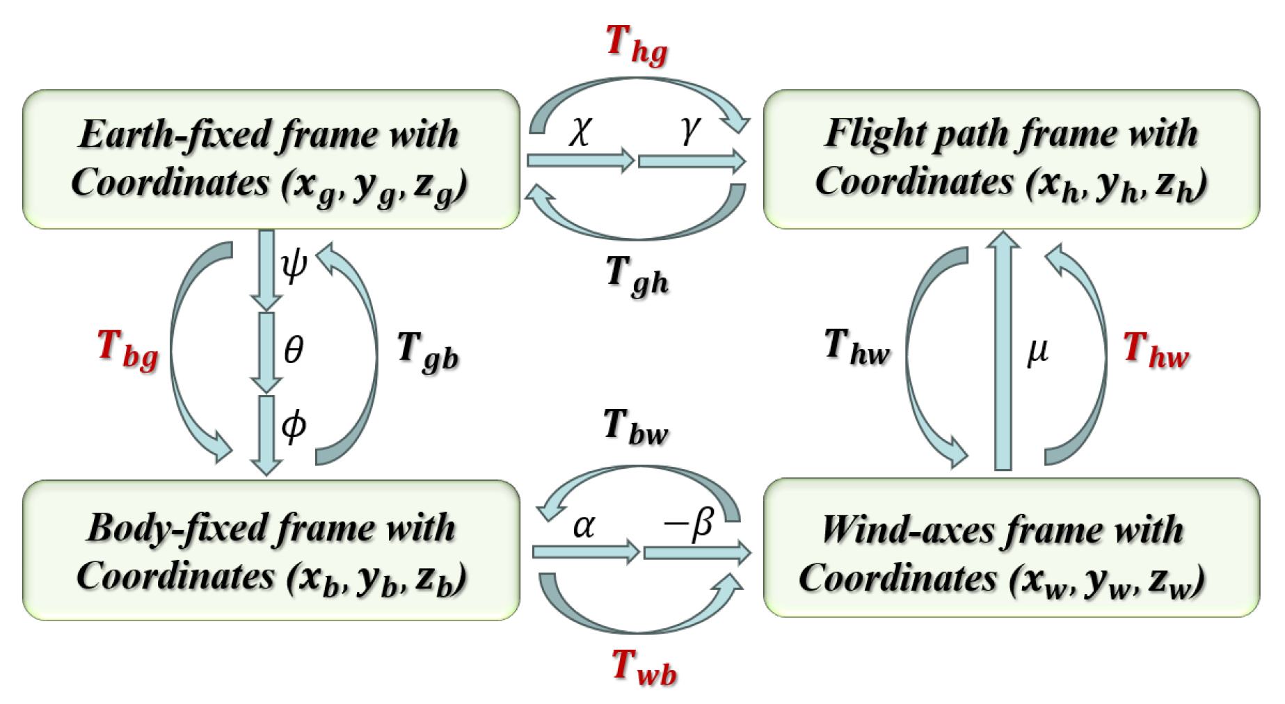
It is assumed that the origin of the body-fixed frame is fixed to the rigid fuselage (definitions of different frames can be found in [27] and are shown in Figure 1). In the symmetrical wing morphing process, geometry alteration produces a shift in the center of gravity (CG) of the aircraft that is no longer located at the origin point. According to the multi-body dynamics theory in [28], the dynamics equations of an aircraft with variable wings can be expressed in vector form as:

$$\left\{\begin{array}{cc}\hfill \mathit{F}=& m\left(\dot{\mathit{V}}+\mathit{\omega }\times \mathit{V}\right)+\frac{\delta \mathit{\omega }}{\delta t}\times \mathit{S}+2\mathit{\omega }\times \frac{\delta \mathit{S}}{\delta t}+\mathit{\omega }\times (\mathit{\omega }\times \mathit{S})+\frac{{\delta }^2\mathit{S}}{\delta t^2}\hfill \\ \hfill \mathit{M}=& \mathit{J}·\frac{\delta \mathit{\omega }}{\delta t}+\frac{\delta \mathit{J}}{\delta t}·\mathit{\omega }+\mathit{\omega }\times (\mathit{J}·\mathit{\omega })+\mathit{S}\times \frac{\delta \mathit{V}}{\delta t}+\mathit{S}\times (\mathit{\omega }\times \mathit{V})\hfill \\ \hfill & +\sum _{i=1}^2\left\{{\mathit{J}}_i·\frac{\delta {\mathit{\omega }}_i}{\delta t}+\frac{\delta {\mathit{J}}_i}{\delta t}·{\mathit{\omega }}_i+{\mathit{\omega }}_{\mathit{i}}\times \left({\mathit{J}}_i·{\mathit{\omega }}_i\right)+\frac{1}{m_{w_i}}\left[{\mathit{S}}_i\times \frac{{\delta }^2{\mathit{S}}_i}{\delta t^2}+\mathit{\omega }\times \left({\mathit{S}}_i\times \frac{\delta {\mathit{S}}_i}{\delta t}\right)\right]\right\},\hfill \end{array}\right.$$

(1)

where $i=1,2$ stands for the left and right wings, respectively. $\mathit{F}$ and $\mathit{M}$ are resultant external force and moment. $\mathit{F}={\mathit{F}}_a+{\mathit{F}}_g+{\mathit{F}}_t$ and $\mathit{M}={\mathit{M}}_a+{\mathit{M}}_g$, where ${\mathit{F}}_a$, ${\mathit{F}}_g$ and ${\mathit{F}}_t$ are aerodynamic force, gravity, and thrust, respectively, and ${\mathit{M}}_a$, ${\mathit{M}}_g$ are aerodynamic moment and the moment caused by gravity, respectively. $\mathit{V}={[u,v,w]}^T$ is the flight velocity and $\mathit{\omega }={[p,q,r]}^T$ the angular velocity; $\mathit{J}$ is the inertia matrix; $\mathit{S}={[S_x,S_y,S_z]}^T$ is the static moment. ${\mathit{\omega }}_i={[{\omega }_{ix},{\omega }_{iy},{\omega }_{iz}]}^T$ and ${\mathit{S}}_i={[S_{ix},S_{iy},S_{iz}]}^T$ are the rotational angular velocity and static moment of each wing, respectively. As the mass distribution and the shape changes of the left and right wings are symmetrical, ${\mathit{\omega }}_i$ and ${\mathit{S}}_i$ can be expressed as [1]:

$$\left\{\begin{array}{c}{\mathit{S}}_1=S_{1x}\mathit{i}+S_{1y}\mathit{j}+S_{1z}\mathit{k}\hfill \\ {\mathit{S}}_2=S_{1x}\mathit{i}-S_{1y}\mathit{j}+S_{1z}\mathit{k}\hfill \end{array}\right.$$

(2)

$$\left\{\begin{array}{c}{\mathit{\omega }}_1={\omega }_{1x}\mathit{i}+{\omega }_{1y}\mathit{j}+{\omega }_{1z}\mathit{k}\hfill \\ {\mathit{\omega }}_2=-{\omega }_{1x}\mathit{i}+{\omega }_{1y}\mathit{j}-{\omega }_{1z}\mathit{k}.\hfill \end{array}\right.$$

(3)

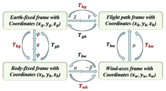
Figure 1. Reference frames and transformation [2].

2.2. Dynamics Model of Morphing Aircraft

The dynamics model of an aircraft is often considered to be a typical singular perturbation system due to the presence of distinct time scales in its dynamics, which means that the motion states of an aircraft exhibit multi-temporal properties. Inspired by [29], flight states variables are divided into three groups: the fast variables of angular velocity p, q, r, the slow variables of attitude angle $\alpha$, $\beta$, $\mu$, and the slowest variables of speed and track angle V, $\gamma$, $\chi$. Accordingly, the equations of motion of the vehicle are depicted as three sets of nonlinear differential equations.

2.2.1. Dynamics Equations of V, $\gamma$, and $\chi$

In the flight path frame, Equation (1) can be rearranged in the following form:

$$\left[\begin{array}{c}{F}_x^h\\ F_y^h\\ F_z^h\end{array}\right]=m(\dot{\mathit{V}}+\mathit{\omega }\times \mathit{V})=m\left(\left[\begin{array}{c}\dot{V}\hfill \\ 0\hfill \\ 0\hfill \end{array}\right]+\left[\begin{array}{c}-\dot{\chi }sin\gamma \\ \dot{\gamma }\\ \dot{\chi }cos\gamma \end{array}\right]\times \left[\begin{array}{c}V\hfill \\ 0\hfill \\ 0\hfill \end{array}\right]\right)=\left[\begin{array}{c}m\dot{V}\\ mVcos\gamma \dot{\chi }\\ -mV\dot{\gamma },\end{array}\right]$$

(4)

where $F_x^h$, $F_y^h$, and $F_z^h$ are components of resultant force vector ${\mathit{F}}_{all}=\mathit{F}+{\mathit{F}}_i$ on the flight path frame, where ${\mathit{F}}_{\mathit{i}}=-\left(\frac{\delta \mathit{\omega }}{\delta t}\times \mathit{S}+2\mathit{\omega }\times \frac{\delta \mathit{S}}{\delta t}+\mathit{\omega }\times (\mathit{\omega }\times \mathit{S})+\frac{{\delta }^2\mathit{S}}{\delta t^2}\right)$ is the inertial force. $\gamma$ and $\chi$ are flight path angle and kinematic azimuth angle, respectively. Then, the derivatives of V, $\gamma$, and $\chi$ can be derived as:

$$\left[\begin{array}{c}\dot{V}\\ \dot{\chi }\\ \dot{\gamma }\end{array}\right]=\left[\begin{array}{ccc}\frac{1}{m}& 0& 0\\ 0& \frac{1}{mVcos\gamma }& 0\\ 0& 0& \frac{-1}{mV}\end{array}\right]\left[\begin{array}{c}{F}_x^h\\ F_y^h\\ F_z^h.\end{array}\right]$$

(5)

${\left[F_x^h,F_y^h,F_z^h\right]}^T$ including aerodynamic force, gravity, thrust, and inertial force can be derived as:

$$\left[\begin{array}{c}{F}_x^h\hfill \\ F_y^h\hfill \\ F_z^h\hfill \end{array}\right]={\mathit{T}}_{hw}{\mathit{T}}_{wb}\left(\left[\begin{array}{c}{F}_{ix}\hfill \\ F_{iy}\hfill \\ F_{iz}\hfill \end{array}\right]+\left[\begin{array}{c}{F}_{tx}\hfill \\ F_{ty}\hfill \\ F_{tz}\hfill \end{array}\right]\right)+{\mathit{T}}_{hw}\left[\begin{array}{c}-D\\ Y\\ -L\end{array}\right]+{\mathit{T}}_{he}\left[\begin{array}{c}0\\ 0\\ mg,\end{array}\right]$$

(6)

where ${\mathit{T}}_{hb}$, ${\mathit{T}}_{hw}$, and ${\mathit{T}}_{he}$ are transformation matrices between different frames, which have been defined in Figure 1 and:

$$T_{hw}=\left[\begin{array}{ccc}1& 0& 0\\ 0& cos\mu & -sin\mu \\ 0& sin\mu & cos\mu \end{array}\right]$$

(7)

$${\mathit{T}}_{wb}=\left[\begin{array}{ccc}cos\alpha cos\beta & sin\beta & sin\alpha cos\beta \\ -cos\alpha sin\beta & cos\beta & -sin\alpha sin\beta \\ -sin\alpha & 0& cos\alpha \end{array}\right]$$

(8)

and

$${\mathit{T}}_{he}=\left[\begin{array}{ccc}cos\chi cos\gamma & -sin\chi & cos\chi sin\gamma \\ sin\chi cos\gamma & cos\chi & sin\chi sin\gamma \\ -sin\gamma & 0& cos\gamma ,\end{array}\right]$$

(9)

where $\alpha$, $\beta$, and $\mu$ are the angle of attack, sideslip angle, and kinematic bank angle, respectively. Further, $F_{ix}$, $F_{iy}$, and $F_{iz}$ and $F_{tx}$, $F_{ty}$, and $F_{tz}$ are components of inertial force and thrust in a body-fixed frame:

$$\left\{\begin{array}{c}{F}_{ix}=-\left(\dot{q}{S}_z-\dot{r}{S}_y+2\left(q{\dot{S}}_z-r{\dot{S}}_y\right)+q\left(p{S}_y-q{S}_x\right)-r\left(r{S}_x-p{S}_z\right)+{\ddot{S}}_x\right)\hfill \\ F_{iy}=-\left(\dot{r}{S}_x-\dot{p}{S}_z+2\left(r{\dot{S}}_x-p{\dot{S}}_z\right)+r\left(q{S}_z-r{S}_y\right)-p\left(p{S}_y-q{S}_x\right)+{\ddot{S}}_y\right)\hfill \\ F_{iz}=-\left(\dot{p}{S}_y-\dot{r}{S}_x+2\left(q{\dot{S}}_y-r{\dot{S}}_x\right)+p\left(r{S}_x-p{S}_z\right)-q\left(q{S}_z-p{S}_y\right)+{\ddot{S}}_z\right)\hfill \end{array}\right.$$

(10)

and

$$\left\{\begin{array}{c}{F}_{tx}=Tcos\phi \hfill \\ F_{ty}=0\hfill \\ F_{tz}=-Tsin\phi ,\hfill \end{array}\right.$$

(11)

where T is the value of thrust and $\phi$ the engine mounting angle (in this paper, $\phi =0$). Furthermore, the aerodynamic force drag D, side force Y, and lift L in the wind-axes frame can be obtained as follows:

$$\left\{\begin{array}{c}L=\overline{q}{S}_{ref}(\Lambda )C_L=\overline{q}{S}_{ref}(\Lambda )\left(C_{L_0}(Ma,\alpha ,\Lambda )+C_{L_{\alpha }}(Ma,\alpha ,\Lambda )\alpha +\frac{\overline{c}(\Lambda )}{2V}{C}_{L_q}(Ma,\alpha ,\Lambda )q\right)\hfill \\ D=\overline{q}{S}_{ref}(\Lambda )C_D=\overline{q}{S}_{ref}(\Lambda )\left(C_{D_0}(Ma,\Lambda )+K(Ma,\Lambda )C_L^2\right)\hfill \\ Y=\overline{q}{S}_{ref}(\Lambda )C_Y=\overline{q}{S}_{ref}(\Lambda )\left(C_{Y\beta }(Ma,\alpha ,\Lambda )\beta +\frac{b(\Lambda )}{2V}\left(C_{Yr}(Ma,\alpha ,\Lambda )r+C_{Yp}(Ma,\alpha ,\Lambda )p\right)\right),\hfill \end{array}\right.$$

(12)

where $\overline{q}$ is the dynamic pressure and $Ma$ is the Mach number, $C_L$, $C_D$, and $C_Y$ are aerodynamic force coefficients, and $C_{L_{\alpha }}$, $C_{L_0}$, $C_{L_q}$, $C_{Y\beta }$, $C_{Yr}$, $C_{Yp}$ are aerodynamic derivatives, which are principally functions of $Ma$, $\alpha$, and $\Lambda$ and can be obtained by Datcom directly [30] (to be illustrated shortly). The drag coefficient $C_D$ is given by a function of $C_L$ [31], in which the two parameters $C_{D_0}$ and K are functions of $Ma$ and $\Lambda$; they can be obtained by fitting the values of $C_L$ and $C_D$ calculated by Datcom.

2.2.2. Dynamic Equations of $\alpha$, $\beta$, and $\mu$

The dynamics equations of $\alpha$, $\beta$, and $\mu$ can be expressed as follows (see [32] for more details):

$$\left[\begin{array}{c}\dot{\alpha }\\ \dot{\beta }\\ \dot{\mu }\end{array}\right]={\left(\begin{array}{ccc}sin\alpha cos\beta & 0& -cos\alpha \\ sin\beta & 1& 0\\ cos\alpha sin\beta & 0& sin\alpha \end{array}\right)}^{-1}\left({\mathit{T}}_{bw}{\mathit{T}}_{wh}\left[\begin{array}{c}-\dot{\chi }sin\gamma \\ \dot{\gamma }\\ \dot{\chi }cos\gamma \end{array}\right]+\left[\begin{array}{c}p\\ q\\ r.\end{array}\right]\right)$$

(13)

2.2.3. Dynamic Equations of p, q, and r

The dynamic equations of ${[p,q,r]}^T$ can be obtained by rewriting Equation (1):

$$\left[\begin{array}{c}\dot{p}\\ \dot{q}\\ \dot{r}\end{array}\right]={\mathit{J}}^{-1}\left({\mathit{M}}_a+{\mathit{M}}_g+{\mathit{M}}_i-\mathit{\omega }\times (\mathit{J}·\mathit{\omega })\right).$$

(14)

Denote ${\mathit{M}}_a={\left[l_a,m_a,n_a\right]}^T$, ${\mathit{M}}_g={\left[l_g,m_g,n_g\right]}^T$, and ${\mathit{M}}_i={\left[l_i,m_i,n_i\right]}^T$; the components can be expressed as [1]:

$$\left\{\begin{array}{c}{l}_a=\overline{q}{S}_{ref}(\Lambda )b(\Lambda )C_l(Ma,\alpha ,\Lambda )\hfill \\ m_a=\overline{q}{S}_{ref}(\Lambda )\overline{c}(\Lambda )C_m(Ma,\alpha ,\Lambda )\hfill \\ n_a=\overline{q}{S}_{ref}(\Lambda )b(\Lambda )C_n(Ma,\alpha ,\Lambda ),\hfill \end{array}\right.$$

(15)

where $C_l$, $C_m$, and $C_n$ are aerodynamic moment coefficients:

$$\left\{\begin{array}{cc}\hfill C_l=& C_{l_{\beta }}(Ma,\alpha ,\Lambda )\beta +\frac{b(\Lambda )}{2V}\left(C_{l_r}(Ma,\alpha ,\Lambda )r+C_{l_p}(Ma,\alpha ,\Lambda )p\right)+\hfill \\ \hfill & C_{l_{{\delta }_a}}(Ma,\alpha ,\Lambda ){\delta }_a+C_{l_{{\delta }_r}}(Ma,\alpha ,\Lambda ){\delta }_r\hfill \\ \hfill C_m=& C_{m_{\alpha }}(Ma,\alpha ,\Lambda )\alpha +\frac{\overline{c}(\Lambda )}{2V}\left(C_{m_q}(Ma,\alpha ,\Lambda )q+C_{m_{\dot{\alpha }}}(Ma,\alpha ,\Lambda )\dot{\alpha }\right)+\hfill \\ \hfill & C_{m_{{\delta }_e}}(Ma,\alpha ,\Lambda ){\delta }_e\hfill \\ \hfill C_n=& C_{n_{\beta }}(Ma,\alpha ,\Lambda )\beta +\frac{b(\Lambda )}{2V}\left(C_{n_r}(Ma,\alpha ,\Lambda )r+C_{n_p}(Ma,\alpha ,\Lambda )p\right)+\hfill \\ \hfill & C_{n_{{\delta }_a}}(Ma,\alpha ,\Lambda ){\delta }_a+C_{n_{{\delta }_r}}(Ma,\alpha ,\Lambda ){\delta }_r,\hfill \end{array}\right.$$

(16)

where $C_{l_{\beta }}$, $C_{l_r}$, $C_{l_p}$, $C_{l_{{\delta }_a}}$, $C_{l_{{\delta }_r}}$, $C_{m_{\alpha }}$, $C_{m_q}$, $C_{m_{\dot{\alpha }}}$, $C_{n_{\beta }}$, $C_{n_r}$, $C_{n_p}$, $C_{n_{{\delta }_a}}$, and $C_{n_{{\delta }_r}}$ are the aerodynamic moment derivatives, ${\delta }_a$, ${\delta }_e$, and ${\delta }_r$ represent control surface input.

$$\left\{\begin{array}{c}{l}_g=S_{y}gcos\varphi cos\theta -S_{z}gsin\varphi cos\theta \hfill \\ m_g=-S_{z}gsin\theta -S_{x}gcos\varphi cos\theta \hfill \\ n_g=S_{x}gsin\varphi cos\theta +S_{y}gsin\theta \hfill \end{array}\right.$$

(17)

$\varphi$ and $\theta$ are roll and pitch angle.

$$\left\{\begin{array}{cc}\hfill l_i=& -\left({\dot{J}}_{x}p-{\dot{J}}_{xy}q-{\dot{J}}_{zx}r+S_y\dot{w}-S_z\dot{v}+S_y(pv-qu)-S_z(ru-pw)\right)\hfill \\ \hfill & -\left(\sum _{n=1}^2\frac{1}{m_{w_i}}\left[S_{iy}{\ddot{S}}_{iz}-S_{iz}{\ddot{S}}_y+q\left(S_{ix}{\dot{S}}_{iy}-S_{iy}{\dot{S}}_{ix}\right)-r\left(S_{iz}{\dot{S}}_{ix}-S_{ix}{\dot{S}}_{iz}\right)\right]\right)\hfill \\ \hfill m_i=& -\left({\dot{J}}_{xy}p+{\dot{J}}_{y}q-{\dot{J}}_{yz}r+S_z\dot{u}-S_x\dot{w}+S_z(qw-rv)-S_x(pv-qu)\right)\hfill \\ \hfill & -\left(\sum _{i=1}^2\frac{1}{m_{w_i}}\left[S_{iz}{\ddot{S}}_{ix}-S_{ix}{\ddot{S}}_{iz}+r\left(S_{iy}{\dot{S}}_{iz}-S_{iz}{\dot{S}}_{iy}\right)-p\left(S_{ix}{\dot{S}}_{iy}-S_{iy}{\dot{S}}_{ix}\right)\right]\right)\hfill \\ \hfill n_i=& -\left({\dot{J}}_{zx}p-{\dot{J}}_{yz}q+{\dot{J}}_{z}r+S_x\dot{v}-S_y\dot{u}+S_x(ru-pw)-S_y(qw-rv)\right)\hfill \\ \hfill & -\left(\sum _{i=1}^2\frac{1}{m_{w_i}}\left[S_{iz}{\ddot{S}}_{ix}-S_{ix}{\ddot{S}}_{iz}+r\left(S_{iy}{\dot{S}}_{iz}-S_{iz}{\dot{S}}_{iy}\right)-p\left(S_{ix}{\dot{S}}_{iy}-S_{iy}{\dot{S}}_{ix}\right)\right]\right).\hfill \end{array}\right.$$

(18)

2.3. Data Acquisition in Symmetry Morphing Process

During the shape variation process, the configuration parameters and aerodynamic derivatives are changing. The geometric parameters related to different configurations, such as the CG position, the root and tip chord of wings, b, $\overline{c}$, and $S_{ref}$ can be found in [25,26]; then we construct one-dimensional lookup tables based on the geometric parameters of six configurations, and interpolation is used to obtain the datas during configuration transition. In addition, the derivatives of $\mathit{S}$, ${\mathit{S}}_i$, $\mathit{J}$, and ${\mathit{J}}_i$ can be calculated by the method in [2,33].

The aerodynamic derivatives of six configurations ($\Lambda ={15.97}^{\circ },{25}^{\circ },{35}^{\circ },{45}^{\circ },{55}^{\circ },{65}^{\circ }$) are calculated by Datcom [30] and the data required in the Datcom input files have been provided in Appendix B of [25,26]. The data obtained from Datcom output files form multi-dimension lookup-tables with respect to Mach number, $\alpha$, and $\Lambda$, which are combined with an interpolation algorithm and may then be constructed for simulation purposes.

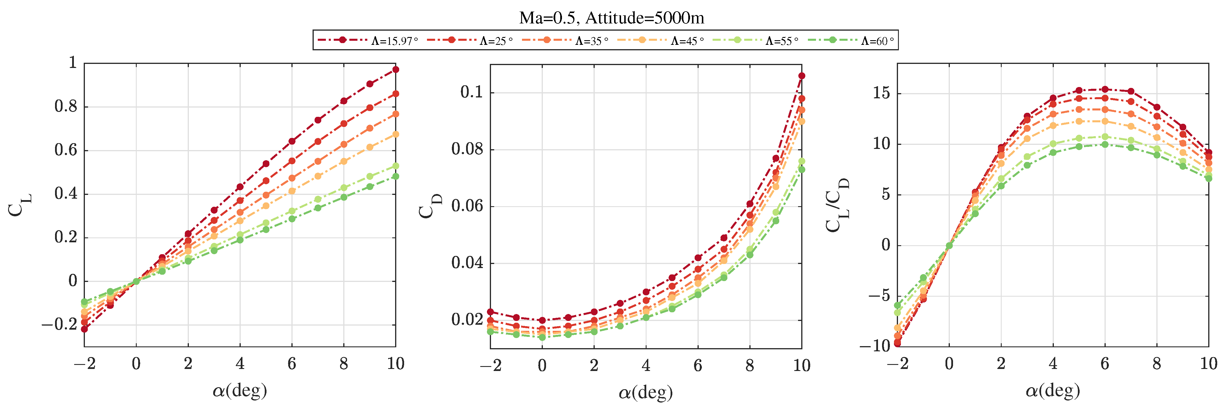
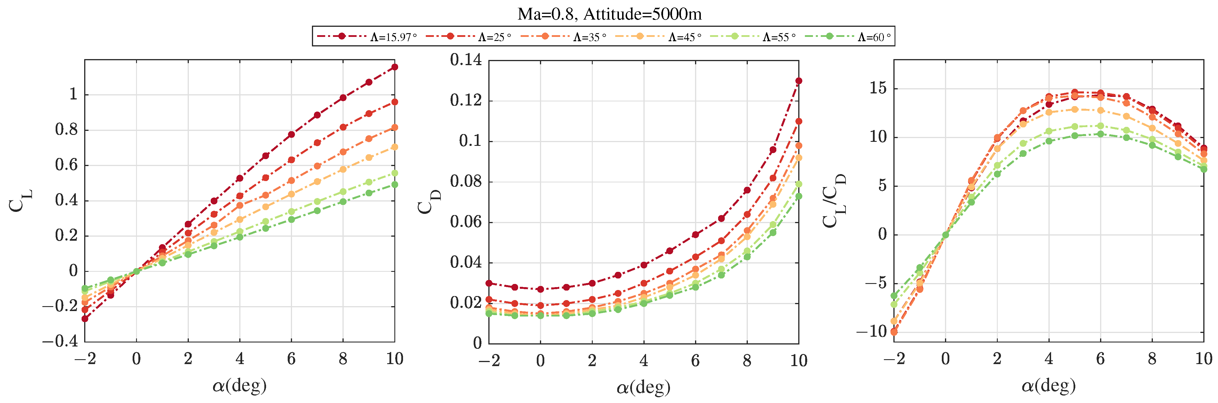
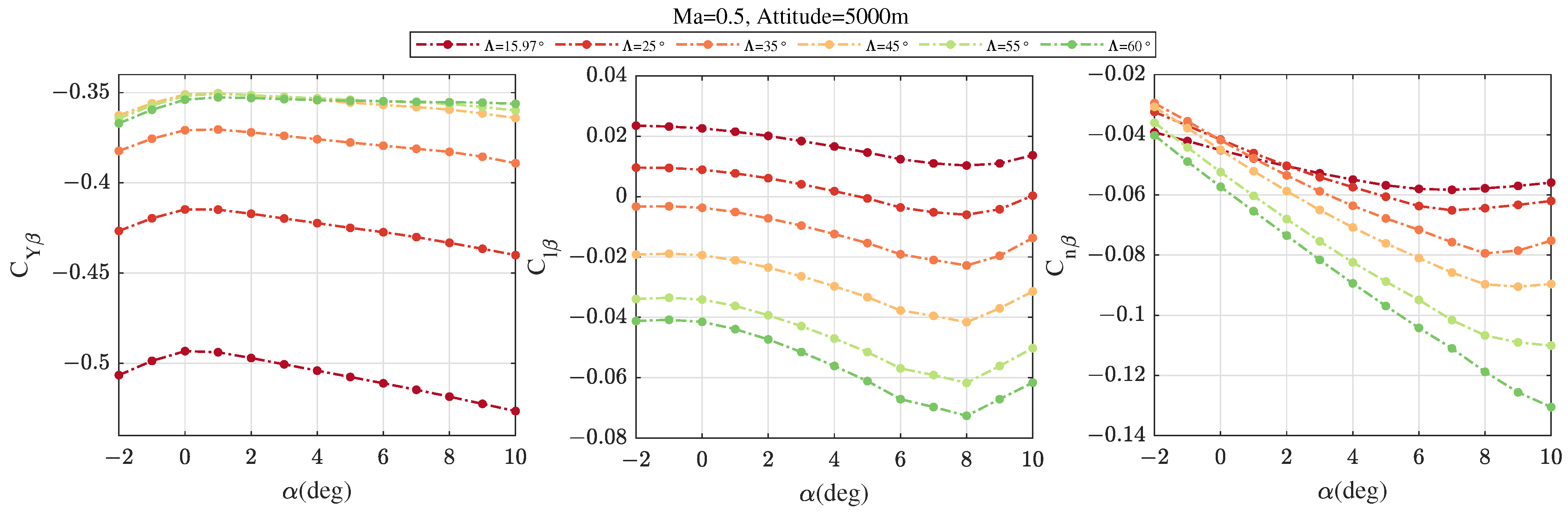
Figure 2 and Figure 3 show the changes of $C_L$, $C_D$, and $C_L/C_D$ under different flight conditions and sweep angle $\Lambda$. At the condition of $Ma$ = 0.5 and attitude = 5000 m, $C_L$ and $C_D$ increase with the growing of $\alpha$ when $\alpha >0$. Additionally, $C_L$, $C_D$, and $C_L/C_D$ decrease when the sweep angle is increasing at the same $\alpha$; when $Ma$ rises to 0.8, the values of $C_L$ and $C_D$ at the same $\alpha$ have increased but the relative changes are generally the same. The difference is mainly reflected in $C_L/C_D$. Figure 4 shows some typical lateral aerodynamic derivatives. It demonstrates that sweep angle has a significant effect on lateral parameters, especially $C_{l_{\beta }}$, the value of which changes from positive to negative as the sweep angle increases. But the variation trend of lateral parameters under different sweep angles is generally the same.

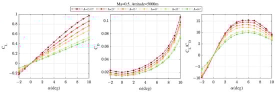
Figure 2. $C_L$, $C_D$, and $C_L/C_D$ at $Ma$ = 0.5, attitude = 5000 m.

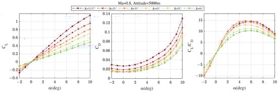
Figure 3. $C_L$, $C_D$, and $C_L/C_D$ at $Ma$ = 0.8, attitude = 5000 m.

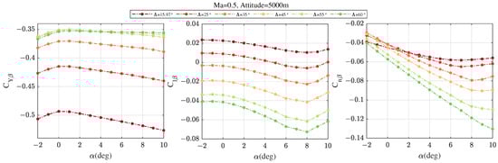
Figure 4. $C_{Y_{\beta }}$, $C_{l_{\beta }}$, and $C_{n_{\beta }}$ at $Ma$ = 0.5, attitude = 5000 m.

3. Dynamic Inversion (DI) Design for Decoupling

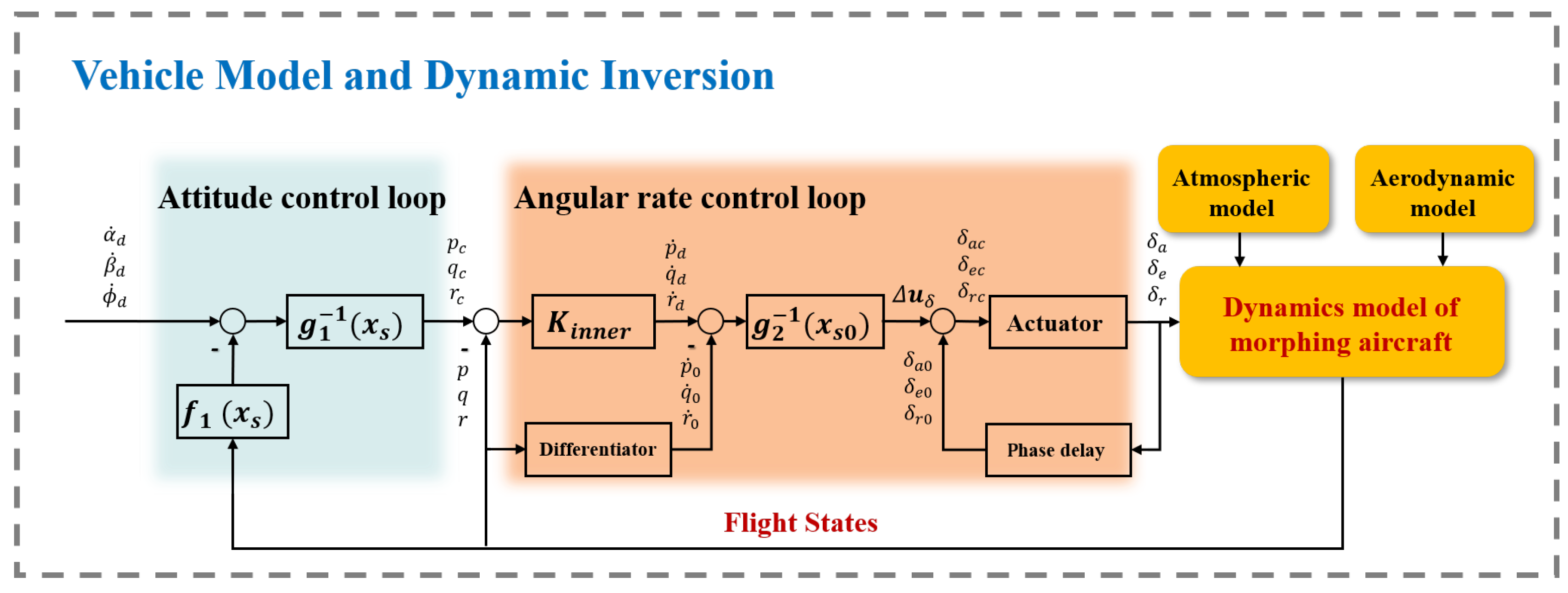
As compared to conventional aircraft, a morphing aircraft is a more complicated nonlinear system requiring a flight controller with outstanding robustness and control accuracy. The typical design approach of a flight control system is to establish a control loop to stabilize vehicle attitude $\alpha$, $\beta$, $\mu$ and angular rates p, q, r in an inner loop, while an outer loop tracks vehicle position (V, $\gamma$, $\chi$ and x, y, z).

Section 2 has established a complete dynamics model of a morphing aircraft, considering that the attitude stability of the inner loop is the basis of position tracking. In this section, we mainly focus on the control of attitude angles $\alpha$, $\beta$, and $\mu$ and angular velocity p, q, and r to realize decoupling control of vehicle attitude. We use INDI and NDI to design a dynamic inversion controller, which is based on a cascaded design with an angular rate control loop and an attitude control loop. Each loop involves one set of equations in Section 2, with three inputs and three outputs.

3.1. Dynamic Inversion Design for the Attitude Control Loop

The objective of the attitude loop controller is to obtain expected ${\left[p_c,q_c,r_c\right]}^T$. The relation between $\alpha$, $\beta$, $\mu$ and p, q, r is based on a kinematic equation independent of vehicle dynamics, so NDI is employed to design the control law instead of INDI [34]. Equation (13) can be expanded as follows:

$$\left[\begin{array}{c}\dot{\alpha }\\ \dot{\beta }\\ \dot{\mu }\end{array}\right]=\underset{f_1\left({\mathit{x}}_s\right)}{\underbrace{-{\left(\begin{array}{ccc}sin\alpha cos\beta & 0& -cos\alpha \\ sin\beta & 1& 0\\ cos\alpha sin\beta & 0& sin\alpha \end{array}\right)}^{-1}{\mathit{T}}_{bw}{\mathit{T}}_{wh}\left[\begin{array}{c}-\dot{\chi }sin\gamma \\ \dot{\gamma }\\ \dot{\chi }cos\gamma \end{array}\right]}}+\underset{g_1\left({\mathit{x}}_s\right)}{\underbrace{{\left(\begin{array}{ccc}sin\alpha cos\beta & 0& -cos\alpha \\ sin\beta & 1& 0\\ cos\alpha sin\beta & 0& sin\alpha \end{array}\right)}^{-1}}}\underset{{\mathit{u}}_{\omega }}{\underbrace{\left[\begin{array}{c}p\\ q\\ r\end{array}\right]}},$$

(19)

where ${\mathit{x}}_s$ is the flight state and ${\mathit{u}}_{\omega }={[p,q,r]}^T$, ${\mathit{T}}_{bw}$, and ${\mathit{T}}_{wh}$ are the inverse of ${\mathit{T}}_{wb}$ and ${\mathit{T}}_{hw}$, respectively. $f_1\left({\mathit{x}}_s\right)$ and $g_1\left({\mathit{x}}_s\right)$ are the matrices of the attitude control loop. The method to calculate $\dot{\gamma }$ and $\dot{\chi }$ in actual flight are given in (A1) and (A2) in Appendix A. Then, the NDI control law is derived:

$$\left[\begin{array}{c}{p}_c\hfill \\ q_c\hfill \\ r_c\hfill \end{array}\right]=g_1^{-1}\left({\mathit{x}}_s\right)\left({\mathit{v}}_1-f_1\left({\mathit{x}}_s\right)\right),$$

(20)

where the ${\mathit{v}}_1={[{\dot{\alpha }}_d,{\dot{\beta }}_d,{\dot{\mu }}_d]}^T$ is the desired dynamics of ${[\dot{\alpha },\dot{\beta },\dot{\mu }]}^T$, which is computed by the adaptive controller from the outer layer, to be introduced shortly.

3.2. Dynamic Inversion Design for the Angular Rate Control Loop

The objective of the angular rate control loop controller is to generate the expected control surface input ${\delta }_a$, ${\delta }_e$, ${\delta }_r$ and INDI is adopted to design the control law. Nonlinear dynamics equations of this loop can be written as:

$$\begin{array}{c}\left[\begin{array}{c}\dot{p}\\ \dot{q}\\ \dot{r}\end{array}\right]={\mathit{J}}^{-1}\left({\mathit{M}}_a+{\mathit{M}}_g+{\mathit{M}}_{\mathrm{i}}-\mathit{\omega }\times (\mathit{J}·\mathit{\omega })\right)\hfill \\ =\underset{f_2\left({\mathit{x}}_s\right)}{\underbrace{{\mathit{J}}^{-1}\left\{\left[\begin{array}{c}{l}_{a_0}\hfill \\ m_{a_0}\hfill \\ n_{a_0}\hfill \end{array}\right]-\mathit{\omega }\times (\mathbf{J}·\mathit{\omega })\right\}}}+\underset{g_2\left({\mathit{x}}_s\right)}{\underbrace{{\mathit{J}}^{-1}\overline{q}S\left[\begin{array}{ccc}b{C}_{l_{{\delta }_a}}& 0& b{C}_{l_{{\delta }_r}}\\ 0& c{C}_{m_{{\delta }_e}}& 0\\ b{C}_{n_{{\delta }_a}}& 0& b{C}_{n_{{\delta }_r}}\end{array}\right]}}\underset{{\mathit{u}}_{\delta }}{\underbrace{\left[\begin{array}{c}{\delta }_a\\ {\delta }_e\\ {\delta }_r\end{array}\right]}}+\hfill \\ \underset{{\zeta }_2}{\underbrace{{\mathit{J}}^{-1}\left(\left[\begin{array}{c}{l}_g\\ m_g\\ n_g\end{array}\right]+\left[\begin{array}{c}{l}_i\\ m_i\\ n_i\end{array}\right]\right)}},\hfill \end{array}$$

(21)

where ${\mathit{u}}_{\delta }={\left[{\delta }_a,{\delta }_e,{\delta }_r\right]}^T$ is the control surface input, and $l_{a_0}$, $m_{a_0}$, and $n_{a_0}$ are the aerodynamic moments when the deflections of ${\mathit{u}}_{\delta }$ are zero. $f_2\left({\mathit{x}}_s\right)$ denotes the control independent state matrix and $g_2\left({\mathit{x}}_s\right)$ is the control matrix, and ${\zeta }_2$ represents the sum of undesired dynamics in the inner loop.

In sampling time $\Delta t$, Equation (14) is rewritten into a first-order Taylor series expansion, as shown in Equation (22):

$$\left[\begin{array}{c}\dot{p}\\ \dot{q}\\ \dot{r}\end{array}\right]=\left[\begin{array}{c}{\dot{p}}_0\hfill \\ {\dot{q}}_0\hfill \\ {\dot{r}}_0\hfill \end{array}\right]+{\left.\frac{\partial g_2\left({\mathit{x}}_s\right){\mathit{u}}_{\delta }}{\partial {\mathit{u}}_{\delta }}\right|}_{\begin{array}{c}{\mathit{x}}_s={\mathit{x}}_{s0}\\ \delta ={\delta }_0\end{array}}\Delta {\mathit{u}}_{\delta }+{\left.\frac{\partial \left(f_1\left({\mathit{x}}_s\right)+g_2\left({\mathit{x}}_s\right){\mathit{u}}_{\delta }\right)}{\partial {\mathit{x}}_s}\right|}_{\begin{array}{c}{\mathit{x}}_s={\mathit{x}}_{s0}\\ \delta ={\delta }_0\end{array}}\Delta {\mathit{x}}_s+\Delta {\zeta }_2+o\left(\Delta {\mathit{x}}_s^2\right).$$

(22)

Note that ${\mathit{\xi }}_2={\left.\frac{\partial \left(f_2\left({\mathit{x}}_s\right)+g_2\left({\mathit{x}}_s\right){\mathit{u}}_{\delta }\right)}{\partial {\mathit{x}}_s}\right|}_{\begin{array}{c}{\mathit{x}}_s={\mathit{x}}_{s0}\\ \delta ={\delta }_0\end{array}}\Delta {\mathit{x}}_s+\Delta {\zeta }_{inner}+o\left(\Delta {\mathit{x}}_s^2\right)$, and Equation (22) can be further simplified as follows:

$$\left[\begin{array}{c}\dot{p}\hfill \\ \dot{q}\hfill \\ \dot{r}\hfill \end{array}\right]=\left[\begin{array}{c}{\dot{p}}_0\hfill \\ {\dot{q}}_0\hfill \\ {\dot{r}}_0\hfill \end{array}\right]+g_2\left({\mathit{x}}_{s0}\right)\Delta {\mathit{u}}_{\delta }+{\mathit{\xi }}_2.$$

(23)

When the sampling time is small enough, the high-order items $o\left(\Delta {\mathit{x}}_s^2\right)$ and the increment of uncertainties $\Delta {\zeta }_2$ are small. According to the time-scale separation principle, term ${\mathit{\xi }}_2$ can be neglected [35] and the desired deflection of the control surface is obtained as follows:

$$\left[\begin{array}{c}{\delta }_{a_c}\hfill \\ {\delta }_{e_c}\hfill \\ {\delta }_{r_c}\hfill \end{array}\right]=\left[\begin{array}{c}{\delta }_{a_0}\hfill \\ {\delta }_{e_0}\hfill \\ {\delta }_{r_0}\hfill \end{array}\right]+g_2^{-1}\left({\mathit{x}}_{s0}\right)\left({\mathit{v}}_2-\left[\begin{array}{c}{\dot{p}}_0\hfill \\ {\dot{q}}_0\hfill \\ {\dot{r}}_0\hfill \end{array}\right]\right),$$

(24)

where ${\left[{\dot{p}}_0,{\dot{q}}_0,{\dot{r}}_0\right]}^T$ and ${\left[{\delta }_{a_0},{\delta }_{e_0},{\delta }_{r_0}\right]}^T$ are the derivatives of angular rates and control surface inputs in the previous moment, respectively, which can be calculated by using a second-order filter introduced in [27]. Further, the input of the angular rate control loop is ${\mathit{v}}_2={\left[{\dot{p}}_d,{\dot{q}}_d,{\dot{r}}_d\right]}^T$, which represents the desired dynamics of ${\left[\dot{p},\dot{q},\dot{r}\right]}^T$ and is obtained as follows:

$${\mathit{v}}_2={\mathit{K}}_{\mathit{\omega }}\left(\left[\begin{array}{c}{p}_c\hfill \\ q_c\hfill \\ r_c\hfill \end{array}\right]-\left[\begin{array}{c}p\hfill \\ q\hfill \\ r\hfill \end{array}\right]\right),$$

(25)

where ${\mathit{K}}_{\mathit{\omega }}=diag(10,10,10)$ is the matrix of bandwidth and ${\left[p_c,q_c,r_c\right]}^T$ the command signal generated by the attitude control loop.

So far, the model inversion has been achieved and the pseudo-linear composite system is illustrated in Figure 5.

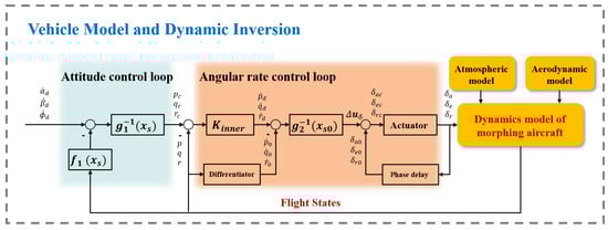
Figure 5. Pseudo-linear composite system architecture.

3.3. Analysis of Dynamic Inversion Controller

In fact, unknown nonlinear disturbances always exist. Here, we assume that there are disturbances that satisfies the following conditions:

Assumption 1. 

The unknown nonlinear disturbance ${\delta }_{d_1}\left(t\right)$ existing in the attitude control loop is continuous and globally bounded.

$$\forall t>0,\exists {\overline{\delta }}_1>0\Rightarrow {\parallel {\delta }_{d_1}\left(t\right)\parallel }_{\infty }\le {\overline{\delta }}_1.$$

(26)

Assumption 2. 

The unknown nonlinear disturbance ${\delta }_{d_2}\left(t\right)$ existing in the angular rate control loop is continuous and globally bounded.

$$\forall t>0,\exists {\overline{\delta }}_2>0\Rightarrow {\parallel {\delta }_{d_2}\left(t\right)\parallel }_{\infty }\le {\overline{\delta }}_2.$$

(27)

Bringing the control law (19) and (24) into (19) and (21), respectively, the dynamics of attitude and angular rate takes the form:

$$\left[\begin{array}{c}\dot{\alpha }\\ \dot{\beta }\\ \dot{\mu }\end{array}\right]={\mathit{f}}_{\mathbf{1}}\left({\mathit{x}}_s\right)+{\mathit{g}}_{\mathbf{1}}\left({\mathit{x}}_s\right)+{\delta }_{d_1}$$

(28)

$$\left[\begin{array}{c}\dot{p}\hfill \\ \dot{q}\hfill \\ \dot{r}\hfill \end{array}\right]=\left[\begin{array}{c}{\dot{p}}_0\hfill \\ {\dot{q}}_0\hfill \\ {\dot{r}}_0\hfill \end{array}\right]+g_2\left({\mathit{x}}_{s0}\right)\Delta {\mathit{u}}_{\delta }+{\mathit{\xi }}_2+{\delta }_{d_2}.$$

(29)

Further,

$$\left[\begin{array}{c}\dot{\alpha }\hfill \\ \dot{\beta }\hfill \\ \dot{\mu }\hfill \end{array}\right]={\mathit{v}}_1+{\delta }_{d_1}$$

(30)

$$\left[\begin{array}{c}\dot{p}\hfill \\ \dot{q}\hfill \\ \dot{r}\hfill \end{array}\right]={\mathit{v}}_2+{\mathit{\xi }}_2+{\delta }_{d_2}.$$

(31)

According to [5], the undesired state response ${\mathit{\xi }}_2$ in the angular rate loop can be effectively reduced when the sample rate is sufficiently high. However, ${\delta }_{d_1}$ and ${\delta }_{d_2}$, including undesired disturbances, cannot be canceled out. Consequently, the desired response dynamics cannot be fully achieved.

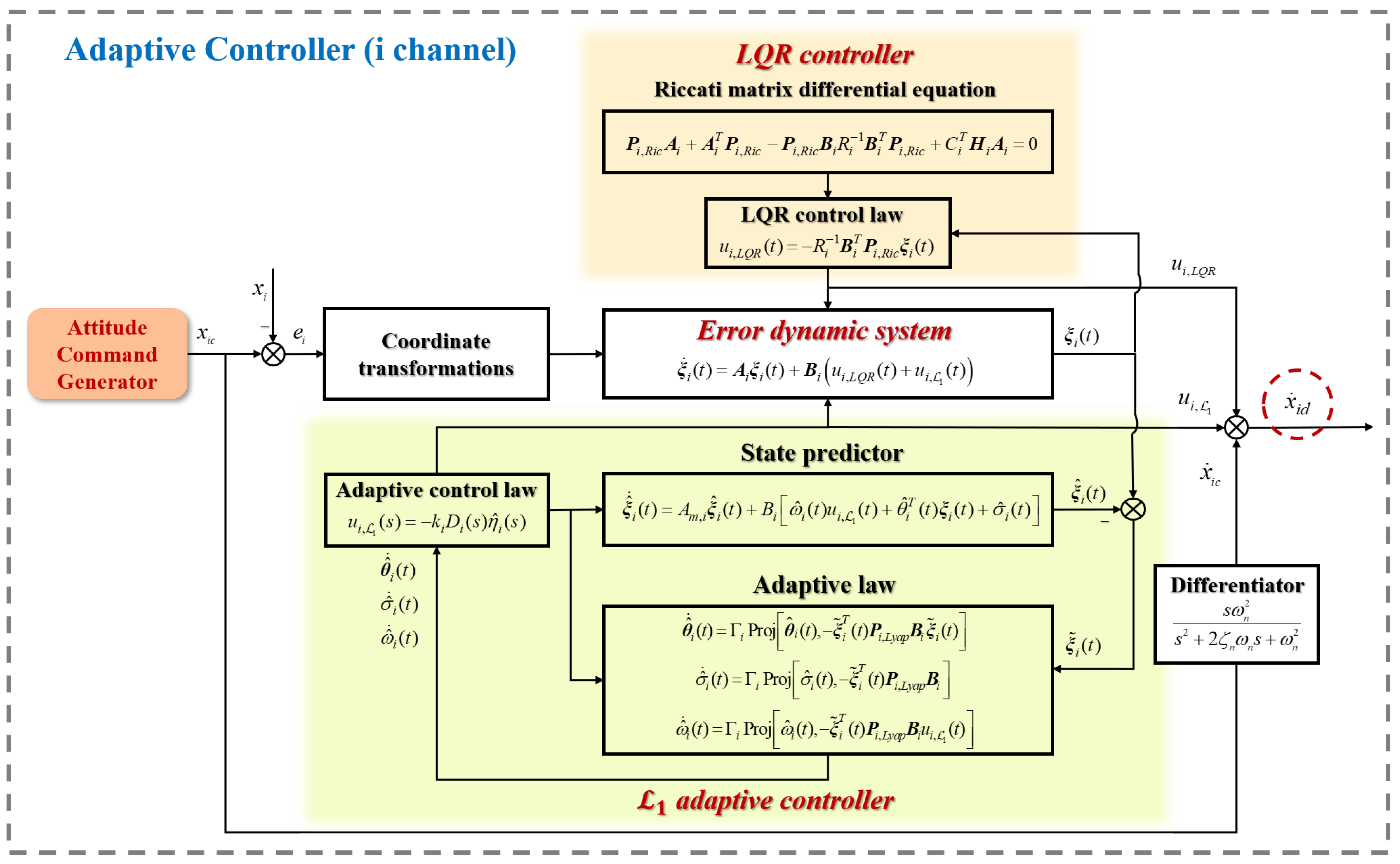
4. Adaptive Flight Controller Design

It can be proven that the nonlinear parts ${\delta }_{d_1}$ and ${\delta }_{d_2}$ are continuous and globally bounded; however, they cannot be eliminated by NDI or INDI completely. As a result of that, the control effect will be decreased greatly. In this section, a linear quadratic regulator (LQR) and ${\mathcal{L}}_1$ adaptive control are adopted to overcome this problem and enhance the benefits from the existing DI controller.

4.1. Error Dynamic System

The ideal linearized system is a simple first-order system, whose transfer function is equivalent to $\frac{1}{Ts}$, and the structure is shown in Figure 5. Inspired by [35], the design of the adaptive controller begins by coordinate transformations. The tracking error is defined as $e_i\left(t\right)=x_i\left(t\right)-x_{ic}\left(t\right)$, $x_i\left(t\right)$ is the actual response, and $x_{ic}\left(t\right)$ is the command of the $\alpha$ channel, $\beta$ channel, or $\mu$ channel, where i represents $\alpha$, $\beta$, or $\mu$. And the error vector of each channel is defined as ${\mathit{\xi }}_i\left(t\right)={\left[{\int }_{t_0}^{t_f}{e}_i\left(t\right)\mathrm{d}t,e_i\left(t\right)\right]}^T$. Then, the single error dynamics system can be defined as follows:

$$\left\{\begin{array}{c}{\mathit{\xi }}_i\left(t\right)={\mathit{A}}_i{\mathit{\xi }}_i\left(t\right)+{\mathit{B}}_i{u}_i\left(t\right)\hfill \\ y_i\left(t\right)={\mathit{C}}_i{\mathit{\xi }}_i\left(t\right),\hfill \end{array}\right.$$

(32)

where ${\mathit{A}}_i=\left[\begin{array}{cc}0\hfill & 1\hfill \\ 0\hfill & 0\hfill \end{array}\right]$, ${\mathit{B}}_i=\left[\begin{array}{c}0\hfill \\ 1\hfill \end{array}\right]$, and ${\mathit{C}}_i=\left[\begin{array}{cc}0\hfill & 1\hfill \end{array}\right]$ are known constant matrices. And

$$u_i\left(t\right)={\dot{e}}_i\left(t\right)={\dot{x}}_i\left(t\right)-{\dot{x}}_{ic}\left(t\right);$$

(33)

then,

$${\dot{x}}_i\left(t\right)=u_i\left(t\right)+{\dot{x}}_{ic}\left(t\right).$$

(34)

Now, we can obtain the control command signal ${\mathit{v}}_1={\left[{\dot{\alpha }}_d,{\dot{\beta }}_d,{\dot{\mu }}_d\right]}^T$ of the attitude loop by (34), in which the control input of error dynamics system $u_i\left(t\right)$ is composed of two parts:

$$u_i\left(t\right)=u_{i,LQR}\left(t\right)+u_{i,{\mathcal{L}}_1}\left(t\right),$$

(35)

where $u_{i,LQR}\left(t\right)$ is the LQR control law and $u_{i,{\mathcal{L}}_1}\left(t\right)$ the ${\mathcal{L}}_1$ adaptive control law, to be defined shortly.

4.2. Linear Quadratic Regulator Controller Design

The LQR controller for $\alpha$, $\beta$, and $\mu$ is designed by employing the LQR method. This method aims at obtaining an optimal feedback gain ${\mathcal{K}}_i$ by minimizing the following objective function $J_i$ [36]:

$$J_i={\int }_0^{\infty }\left({\mathit{\xi }}_i^T\left(t\right){\mathit{H}}_i{\mathit{\xi }}_i\left(t\right)+u_{i,LQR}^T\left(t\right)R_i{u}_{i,LQR}\left(t\right)\right)dt,$$

(36)

where ${\mathit{H}}_i\ge 0$ is the state weight matrix and $R_i>0$ the input weight matrix. The expected control input is:

$$u_{i,LQR}\left(t\right)=-R_i^{-1}{\mathit{B}}_i^T{\mathit{P}}_{i,Ric}{\mathit{\xi }}_i\left(t\right),$$

(37)

where ${\mathit{P}}_{i,Ric}$ is the symmetric definite solution of Riccati matrix differential equation as follows:

$${\mathit{P}}_{i,Ric}{\mathit{A}}_i+{\mathit{A}}_i^T{\mathit{P}}_{i,Ric}-{\mathit{P}}_{i,Ric}{\mathit{B}}_i{R}_i^{-1}{\mathit{B}}_i^T{\mathit{P}}_{i,Ric}+{\mathit{C}}_i^T{\mathit{H}}_i{\mathit{A}}_i=0.$$

(38)

Thus, the feedback gain matrix is obtained as:

$${\mathcal{K}}_i=R_i^{-1}{\mathit{B}}_i^T{\mathit{P}}_{i,Ric}.$$

(39)

Then, the linear feedback control law $u_{i,LQR}$ can be written as:

$$u_{i,LQR}\left(t\right)=-{\mathcal{K}}_i{\mathit{\xi }}_i\left(t\right).$$

(40)

The state weight matrices of $\alpha$, $\beta$, and $\mu$ are selected as ${\mathit{H}}_{\alpha }=\mathit{diag}(0.5,1)$, ${\mathit{H}}_{\beta }=\mathit{diag}(1.1,1)$, and ${\mathit{H}}_{\mu }=\mathit{diag}(1.2,1)$, respectively. And the input weight matrices are selected as $R_{\alpha }=R_{\beta }=R_{\mu }=1$. Then, we can get the feedback gain of the LQR controller: ${\mathcal{K}}_{\alpha }={[0.7071,1.5538]}^T$, ${\mathcal{K}}_{\beta }={[1,1.7321]}^T$, and ${\mathcal{K}}_{\mu }={[1.0954,1.7863]}^T$.

4.3. ${\mathcal{L}}_1$ Adaptive Controller Design

Inspired by [20,22], the feedback gain ${\mathcal{K}}_i$ leads the closed-loop error dynamics system as follows:

$$\left\{\begin{array}{c}{\dot{\mathit{\xi }}}_i\left(t\right)=\left({\mathit{A}}_i-{\mathit{B}}_i{\mathcal{K}}_i\right){\mathit{\xi }}_i\left(t\right)+{\mathit{B}}_i{u}_{i,{\mathcal{L}}_1}\left(t\right)\hfill \\ y_i\left(t\right)={\mathit{C}}_i{\mathit{\xi }}_i\left(t\right),\hfill \end{array}\right.$$

(41)

where ${\mathcal{K}}_i$ renders ${\mathit{A}}_{m,i}\triangleq {\mathit{A}}_i-{\mathit{B}}_i{\mathcal{K}}_i$ Hurwitz matrix. Meanwhile, the uncertainty and disturbance are considered, then the error dynamics system takes the form as follows:

$$\left\{\begin{array}{c}{\dot{\mathit{\xi }}}_i\left(t\right)={\mathit{A}}_{m,i}{\mathit{\xi }}_i\left(t\right)+{\mathit{B}}_i\left({\omega }_i{u}_{i,{\mathcal{L}}_1}\left(t\right)+{\mathit{\theta }}_i^T\left(t\right){\mathit{\xi }}_i\left(t\right)+{\sigma }_i\left(t\right)\right)\hfill \\ y_i\left(t\right)={\mathit{C}}_i{\mathit{\xi }}_i\left(t\right),\hfill \end{array}\right.$$

(42)

where ${\omega }_i\in R$, ${\mathit{\theta }}_i^T\left(t\right)\in R^{2\times 1}$, and ${\sigma }_i\left(t\right)\in R$ are unknown parameters related to time-varying unknown disturbances. Here are some assumptions for ${\mathcal{L}}_1$ adaptive controller design:

Assumption 3. 

Unknown parameters ${\mathit{\theta }}_i^T\left(t\right)$ and ${\sigma }_i\left(t\right)$ are uniformly bounded:

$$\forall t>0,\exists {\Theta }_i>0\Rightarrow {∥{\mathit{\theta }}_i\left(t\right)∥}_{\infty }\le {\Theta }_i$$

(43)

$$\forall t>0,\exists {\Delta }_i>0\Rightarrow {∥{\sigma }_i\left(t\right)∥}_{\infty }\le {\Delta }_i.$$

(44)

Assumption 4. 

The rate of variation of unknown parameters ${\mathit{\theta }}_i^T\left(t\right)$ and ${\sigma }_i\left(t\right)$ is uniformly bounded:

$$\forall t>0\Rightarrow {∥{\dot{\mathit{\theta }}}_i\left(t\right)∥}_{\infty }\le d_{i,\mathit{\theta }}<\infty$$

(45)

$$\forall t>0\Rightarrow {∥{\dot{\sigma }}_i\left(t\right)∥}_{\infty }\le d_{i,\sigma }<\infty .$$

(46)

Assumption 5. 

The uncertain system input gain has known upper and lower bounds:

$$\forall t>0,{\omega }_i\left(t\right)\in {\Omega }_i\triangleq \left[{\omega }_{i,l},{\omega }_{i,u}\right].$$

(47)

According to the assumptions above, the ${\mathcal{L}}_1$ adaptive controller can be obtained.

State predictor

For the error dynamics system proposed in (42), the following state predictor can be established:

$$\left\{\begin{array}{c}{\dot{\widehat{\mathit{\xi }}}}_i\left(t\right)={\mathit{A}}_{m,i}{\widehat{\mathit{\xi }}}_i\left(t\right)+{\mathit{B}}_i\left({\widehat{\omega }}_i\left(t\right)u_{i,{\mathcal{L}}_1}\left(t\right)+{\widehat{\mathit{\theta }}}_i^T\left(t\right){\mathit{\xi }}_i\left(t\right)+{\widehat{\sigma }}_i\left(t\right)\right),{\widehat{\mathit{\xi }}}_i\left(0\right)={[0,0]}^{\mathrm{T}}\hfill \\ {\widehat{y}}_i\left(t\right)={\mathit{C}}_i{\widehat{\mathit{\xi }}}_i\left(t\right),\hfill \end{array}\right.$$

(48)

where ${\widehat{\mathit{\xi }}}_i\left(t\right)$ and ${\widehat{y}}_i\left(t\right)$ are the estimations of states, ${\widehat{\omega }}_i\left(t\right)$, ${\widehat{\mathit{\theta }}}_i^T\left(t\right)$, and ${\widehat{\sigma }}_i\left(t\right)$ are adaptive estimations of ${\omega }_i$, ${\mathit{\theta }}_i^T\left(t\right)$ and ${\sigma }_i\left(t\right)$, respectively.

Adaptation laws

The estimations ${\widehat{\omega }}_i\left(t\right)$, ${\widehat{\mathit{\theta }}}_i^T\left(t\right)$, and ${\widehat{\sigma }}_i\left(t\right)$ are updated by the following projection-based adaptation laws:

$${\dot{\widehat{\mathit{\theta }}}}_i\left(t\right)={\Gamma }_{i}Proj\left[{\widehat{\mathit{\theta }}}_i\left(t\right),-{\tilde{\mathit{\xi }}}_i^T\left(t\right){\mathit{P}}_{\mathit{i},\mathit{Lyap}}{\mathit{B}}_i{\tilde{\mathit{\xi }}}_i\left(t\right)\right],{\widehat{\mathit{\theta }}}_i\left(0\right)={\widehat{\mathit{\theta }}}_{i0}$$

(49)

$${\dot{\widehat{\sigma }}}_i\left(t\right)={\Gamma }_{i}Proj\left[{\widehat{\sigma }}_i\left(t\right),-{\tilde{\mathit{\xi }}}_i^T\left(t\right){\mathit{P}}_{\mathit{i},\mathit{Lyap}}{\mathit{B}}_i\right],{\widehat{\sigma }}_i\left(0\right)={\widehat{\sigma }}_{i0}$$

(50)

$${\dot{\widehat{\omega }}}_i\left(t\right)={\Gamma }_{i}Proj\left[{\widehat{\omega }}_i\left(t\right),-{\tilde{\mathit{\xi }}}_i^T\left(t\right){\mathit{P}}_{\mathit{i},\mathit{Lyap}}{\mathit{B}}_i{u}_{i,{\mathcal{L}}_1}\left(t\right)\right],{\widehat{\omega }}_i\left(0\right)={\widehat{\omega }}_{i0},$$

(51)

where ${\tilde{\mathit{\xi }}}_i\left(t\right)\triangleq {\widehat{\mathit{\xi }}}_i\left(t\right)-{\mathit{\xi }}_i\left(t\right)$ represents the estimation error of ${\mathit{\xi }}_i$, ${\Gamma }_i\in R^{+}$ is the adaptation rate and ${\mathit{P}}_{i,\mathit{Lyap}}$ the solution of the algebraic Lyapunov equation ${\mathit{A}}_{m,i}^T{\mathit{P}}_{\mathit{i},\mathit{Lyap}}+{\mathit{P}}_{\mathit{i},\mathit{Lyap}}{\mathit{A}}_{m,i}=-{\mathit{Q}}_{i,Lyap}$(${\mathit{Q}}_{i,\mathit{Lyap}}>0$), Proj is the projection operator.

Control Law

The control signal $u_{i,{\mathcal{L}}_1}\left(t\right)$ of the ${\mathcal{L}}_1$ adaptive controller is generated by the following control law:

$$u_{i,{\mathcal{L}}_1}\left(s\right)=-k_i{D}_i\left(s\right)\left({\widehat{\eta }}_i\left(s\right)+k_{g_i}{r}_i\left(s\right)\right),$$

(52)

where ${\widehat{\eta }}_i\left(s\right)$ and $r_i\left(s\right)$ are the Laplace transformations of command signal $r_i\left(t\right)$ and ${\widehat{\eta }}_i\left(t\right)\triangleq \widehat{\omega }\left(t\right)u_{{\mathcal{L}}_1}\left(t\right)+{\widehat{\mathit{\theta }}}^T\left(t\right){\mathit{\xi }}_i\left(t\right)+\widehat{\sigma }\left(t\right)$, $k_{g_i}\triangleq {\left({\mathit{C}}_i^T{\mathit{A}}_{m,i}^{-1}{\mathit{B}}_i\right)}^{-1}$ is the feed-forward filter adopted to eliminate the zero steady-state error of the output response, $k_i\in R$ is the filter gain, and $D_i\left(s\right)$ the transfer function of strict true partition:

$${\mathcal{C}}_i\left(s\right)=\frac{{\omega }_i{k}_i{D}_i\left(s\right)}{1+{\omega }_i{k}_i{D}_i\left(s\right)},\forall {\omega }_i\in {\Omega }_i.$$

(53)

Actually, the objective of control is making the states track the command signal well, so the desired value of ${\mathit{\xi }}_i$ is 0, which means $r_i\left(s\right)=0$. Then, the ${\mathcal{L}}_1$ adaptive control law can be simplified as follows:

$$u_{i,{\mathcal{L}}_1}\left(s\right)=-k_i{D}_i\left(s\right){\widehat{\eta }}_i\left(s\right).$$

(54)

Additionally, the following ${\mathcal{L}}_1$ norm condition is required to satisfy to ensure the stability of the closed-loop system:

$${∥G_i\left(s\right)∥}_{{\mathcal{L}}_1}{L}_i<1,$$

(55)

where

$$L_i\triangleq max{∥{\mathit{\theta }}_i∥}_1,{∥{\mathit{\theta }}_i\left(t\right)∥}_{\infty }\le {\Theta }_i$$

(56)

$${\mathcal{H}}_i\left(s\right)\triangleq {\left(s\mathit{I}-{\mathit{A}}_{m,i}\right)}^{-1}{\mathit{B}}_i$$

(57)

$${\Phi }_i\left(s\right)\triangleq {\mathcal{H}}_i\left(s\right)\left(1-{\mathcal{C}}_i\left(s\right)\right).$$

(58)

In this paper, the control parameters of $\alpha$, $\beta$, and $\mu$ are same. The transfer function $D_i=\frac{1}{s}$ and the filter gain $k_i=10$. In the adaptation laws, the parameters are selected as ${\Gamma }_i=10,000$ and ${\mathit{Q}}_{i,Lyap}={\mathit{I}}_{2\times 2}$. Besides that, the projection range of the adaptation laws are set as ${\Theta }_i=3\times {10}^{-3}$, ${\Delta }_i=20$, and ${\Omega }_i\in [0.1,2]$.

So far, we have finished the design of the adaptive controller composed of an LQR controller and a ${\mathcal{L}}_1$ adaptive controller, as shown in Figure 6.

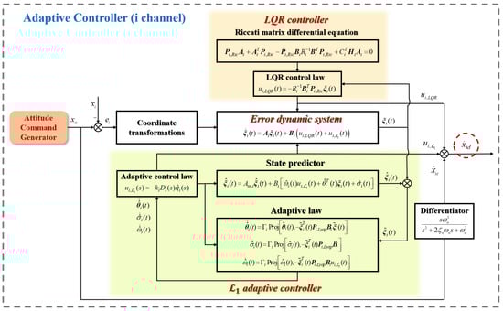
Figure 6. The structure of the adaptive controller based on LQR and ${\mathcal{L}}_1$ adaptive control.

5. Stability Analysis

Focus on the tracking error of $\alpha$, $\beta$, and $\mu$ and consider the following estimation error:

$${\tilde{\mathit{\xi }}}_i\left(t\right)={\widehat{\mathit{\xi }}}_i\left(t\right)-{\mathit{\xi }}_i\left(t\right);$$

(59)

then, we can get the following prediction-error dynamics:

$${\dot{\tilde{\mathit{\xi }}}}_i\left(t\right)={\mathit{A}}_{m,i}{\tilde{\mathit{\xi }}}_i\left(t\right)+{\mathit{B}}_i\left({\tilde{\omega }}_i\left(t\right)u_{i,{\mathcal{L}}_1}\left(t\right)+{\tilde{\mathit{\theta }}}_i^T\left(t\right){\mathit{\xi }}_i\left(t\right)+{\tilde{\sigma }}_i\left(t\right)\right),{\widehat{\mathit{\xi }}}_i\left(0\right)={[0,0]}^{\mathrm{T}},$$

(60)

where

$${\tilde{\omega }}_i\left(t\right)={\widehat{\omega }}_i\left(t\right)-{\omega }_i$$

(61)

$${\tilde{\mathit{\theta }}}_i\left(t\right)={\widehat{\mathit{\theta }}}_i\left(t\right)-{\mathit{\theta }}_i\left(t\right)$$

(62)

$${\tilde{\sigma }}_i\left(t\right)={\widehat{\sigma }}_i\left(t\right)-{\sigma }_i\left(t\right).$$

(63)

Then, the estimation error ${\tilde{\mathit{\xi }}}_i\left(t\right)$ in frequency domain can be written as:

$${\tilde{\mathit{\xi }}}_i\left(s\right)={\mathcal{H}}_i\left(s\right){\tilde{\eta }}_i\left(s\right),$$

(64)

where

$${\tilde{\eta }}_i\left(t\right)={\tilde{\omega }}_i\left(t\right)u_{i,{\mathcal{L}}_1}+{\tilde{\mathit{\theta }}}_i^T\left(t\right){\mathit{\xi }}_i\left(t\right)+{\tilde{\sigma }}_i\left(t\right).$$

(65)

Lemma 1. 

The estimation error ${\tilde{\mathit{\xi }}}_i$ is uniformly bounded,

$$\parallel {\tilde{\mathit{\xi }}}_i{\parallel }_{{\mathcal{L}}_{\infty }}\le \sqrt{\frac{{\Theta }_{m_i}}{{\lambda }_{min}\left(P_{i,Lyap}\right){\Gamma }_i}},$$

(66)

where

$${\Theta }_{m_i}\triangleq 4\left({\left({\omega }_{i,u}-{\omega }_{i,l}\right)}^2+{\Theta }_i^2+{\Delta }_i^2+\frac{{\lambda }_{max}\left(P_{i,Lyap}\right)}{{\lambda }_{min}\left(Q_{i,Lyap}\right)}\left(d_{i,\mathit{\theta }}{\Theta }_i+d_{i,\sigma }{\Delta }_i\right)\right)$$

(67)

and ${\lambda }_{min}\left(P_{i,Lyap}\right)$ and ${\lambda }_{max}\left(P_{i,Lyap}\right)$ are the minimum and maximum eigenvalues of $P_{i,Lyap}$, respectively.

Proof. 

Select the Lyapunov function candidate

$$V({\tilde{\mathit{\xi }}}_i\left(t\right),{\tilde{\mathit{\theta }}}_i\left(t\right),{\tilde{\omega }}_i\left(t\right),{\tilde{\sigma }}_i\left(t\right))={\tilde{\mathit{\xi }}}_i^T\left(t\right){\mathit{P}}_{i,Lyap}{\tilde{\mathit{\xi }}}_i\left(t\right)+\frac{1}{{\Gamma }_i}\left({\tilde{\omega }}_i^2\left(t\right)+{\tilde{\mathit{\theta }}}_i^T\left(t\right){\tilde{\mathit{\theta }}}_i\left(t\right)+{\tilde{\sigma }}_i^2\left(t\right)\right).$$

(68)

Firstly, we prove that

$$V_i\left(t\right)\le \frac{{\Theta }_{m_i}}{{\Gamma }_i}.$$

(69)

The derivative of $V_i\left(t\right)$ is

$${\dot{V}}_i\left(t\right)={\dot{\tilde{\mathit{\xi }}}}_i^T\left(t\right){\mathit{P}}_{i,Lyap}{\tilde{\mathit{\xi }}}_i\left(t\right)+{\tilde{\mathit{\xi }}}_i^T\left(t\right){\mathit{P}}_{i,Lyap}{\dot{\tilde{\mathit{\xi }}}}_i\left(t\right)+\frac{2}{{\Gamma }_i}\left({\tilde{\omega }}_i\left(t\right){\dot{\tilde{\omega }}}_i\left(t\right)+{\tilde{\mathit{\theta }}}_i^T\left(t\right){\dot{\tilde{\mathit{\theta }}}}_i\left(t\right)+{\tilde{\sigma }}_i\left(t\right){\dot{\tilde{\sigma }}}_i\left(t\right)\right)$$

(70)

combined with (60) and ${\mathit{A}}_{m,i}^{\mathrm{T}}{\mathit{P}}_{i,Lyap}+{\mathit{P}}_{i,Lyap}{\mathit{A}}_{m,i}=-{\mathit{Q}}_{i,Lyap}$

$$\begin{array}{cc}\hfill \dot{V}\left(t\right)=& -{\tilde{\mathit{\xi }}}_i^T\left(t\right){\mathit{Q}}_{Lyap}{\tilde{\mathit{\xi }}}_i\left(t\right)+2{\mathit{\xi }}_i^T\left(t\right){\mathit{P}}_{i,Lyap}{\mathit{B}}_i\left({\tilde{\omega }}_i\left(t\right)u_{i,{\mathcal{L}}_1}\left(t\right)+{\tilde{\mathit{\theta }}}_i^T\left(t\right){\mathit{\xi }}_i\left(t\right)+{\tilde{\sigma }}_i\left(t\right)\right)\hfill \\ \hfill & +\frac{2}{{\Gamma }_i}\left({\tilde{\omega }}_i\left(t\right)({\dot{\widehat{\omega }}}_i\left(t\right)-0)+{\tilde{\mathit{\theta }}}_i^T\left(t\right)({\dot{\widehat{\mathit{\theta }}}}_i\left(t\right)-{\dot{\mathit{\theta }}}_i\left(t\right))+{\tilde{\sigma }}_i\left(t\right)({\dot{\widehat{\sigma }}}_i\left(t\right)-{\dot{\sigma }}_i\left(t\right))\right)\hfill \end{array}$$

(71)

and (71) can be further written as

$$\begin{array}{cc}\hfill {\dot{V}}_i\left(t\right)=& -{\tilde{\mathit{\xi }}}_i^T\left(t\right){\mathit{Q}}_{i,Lyap}{\tilde{\mathit{\xi }}}_i\left(t\right)\hfill \\ \hfill & +2\left({\tilde{\mathit{\xi }}}_i^T\left(t\right){\mathit{P}}_{i,Lyap}{\mathit{B}}_i{\tilde{\omega }}_i\left(t\right)u_{i,{\mathcal{L}}_1}\left(t\right)+\frac{1}{{\Gamma }_i}{\tilde{\omega }}_i\left(t\right){\dot{\widehat{\omega }}}_i\left(t\right)\right)\hfill \\ \hfill & +2\left({\tilde{\mathit{\xi }}}_i^T\left(t\right){\mathit{P}}_{i,Lyap}{\mathit{B}}_i{\tilde{\mathit{\theta }}}_i^T\left(t\right){\mathit{\xi }}_i\left(t\right)+\frac{1}{{\Gamma }_i}{\tilde{\mathit{\theta }}}_i^T\left(t\right){\dot{\widehat{\mathit{\theta }}}}_i\left(t\right)\right)\hfill \\ \hfill & +2\left({\tilde{\mathit{\xi }}}_i^T\left(t\right){\mathit{P}}_{i,Lyap}{\mathit{B}}_i{\tilde{\sigma }}_i\left(t\right)+\frac{1}{{\Gamma }_i}{\tilde{\sigma }}_i\left(t\right){\dot{\widehat{\sigma }}}_i\left(t\right)\right)\hfill \\ \hfill & -\frac{2}{{\Gamma }_i}\left({\tilde{\mathit{\theta }}}_i^T\left(t\right){\dot{\mathit{\theta }}}_i\left(t\right)+{\tilde{\sigma }}_i\left(t\right){\dot{\sigma }}_i\left(t\right)\right).\hfill \end{array}$$

(72)

The property of the projection operator ensures that [37]

$$\frac{1}{{\Gamma }_i}{\tilde{\omega }}_i\left(t\right){\dot{\widehat{\omega }}}_i\left(t\right)+{\mathit{\xi }}_i^T{\mathit{P}}_{i,Lyap}{\mathit{B}}_i{\tilde{\omega }}_i\left(t\right)u_{i,{\mathcal{L}}_1}\left(t\right)\le 0$$

(73)

$$\frac{1}{{\Gamma }_i}{\tilde{\mathit{\theta }}}_i^{\top }\left(t\right){\dot{\widehat{\mathit{\theta }}}}_i\left(t\right)+{\mathit{\xi }}_i^T\left(t\right){\mathit{P}}_{i,Lyap}{\mathit{B}}_i{\tilde{\mathit{\theta }}}_i^{\top }\left(t\right){\mathit{\xi }}_i\left(t\right)\le 0$$

(74)

$$\frac{1}{{\Gamma }_i}{\tilde{\sigma }}_i\left(t\right){\dot{\widehat{\sigma }}}_i\left(t\right)+{\mathit{\xi }}_i^T\left(t\right){\mathit{P}}_{i,Lyap}{\mathit{B}}_i{\tilde{\sigma }}_i^{\top }\left(t\right)\le 0.$$

(75)

Thus, (72) satisfies the following conditions:

$${\dot{V}}_i\left(t\right)\le -{\tilde{\mathit{\xi }}}_i^T\left(t\right){\mathit{Q}}_{i,Lyap}{\tilde{\mathit{\xi }}}_i\left(t\right)+\frac{2}{{\Gamma }_i}\left(\left|{\tilde{\mathit{\theta }}}_i^T\left(t\right){\dot{\mathit{\theta }}}_i\left(t\right)\right|+\left|{\tilde{\sigma }}_i\left(t\right){\dot{\sigma }}_i\left(t\right)\right|\right).$$

(76)

Assumptions 3 and 4 ensure the boundary and the rate of variation of ${\mathit{\theta }}_i^T\left(t\right)$ and ${\sigma }_i\left(t\right)$ for all $t\ge 0$ and we get

$${\tilde{\mathit{\theta }}}_i^T\left(t\right){\dot{\mathit{\theta }}}_i\left(t\right)+{\tilde{\sigma }}_i\left(t\right){\dot{\sigma }}_i\left(t\right)\le 4\left(d_{i,\mathit{\theta }}{\Theta }_i+d_{i,\sigma }{\Delta }_i\right).$$

(77)

Then, (76) can be simplified to

$${\dot{V}}_i\left(t\right)\le -{\tilde{\mathit{\xi }}}_i^{\top }\left(t\right){\mathit{Q}}_{i,Lyap}{\tilde{\mathit{\xi }}}_i\left(t\right)+\frac{4}{{\Gamma }_i}\left(d_{i,\mathit{\theta }}{\Theta }_i+d_{i,\sigma }{\Delta }_i\right).$$

(78)

When $t=0$, ${\widehat{\mathit{\xi }}}_i\left(0\right)={\mathit{\xi }}_i\left(0\right)$, we can prove that

$$V_i\left(0\right)=\frac{1}{{\Gamma }_i}\left({\tilde{\omega }}_i^2\left(t\right)+{\tilde{\mathit{\theta }}}_i^T\left(t\right){\tilde{\mathit{\theta }}}_i\left(t\right)+{\tilde{\sigma }}_i^2\left(t\right)\right)\le \frac{4}{{\Gamma }_i}\left({\left({\omega }_{i,u}-{\omega }_{i,l}\right)}^2+{\Theta }_i^2+{\Delta }_i^2\right)<\frac{{\Theta }_{m_i}}{{\Gamma }_i}.$$

(79)

Then, we assume that if at any time $\tau >0$,

$$V_i\left(\tau \right)>\frac{{\Theta }_{m_i}}{{\Gamma }_i},$$

(80)

then it follows from (67) and (68) that

$${\tilde{\mathit{\xi }}}_i^T\left(\tau \right){\mathit{P}}_{i,Lyap}{\tilde{\mathit{\xi }}}_i\left(\tau \right)=V_i\left(\tau \right)-\frac{1}{{\Gamma }_i}\left({\tilde{\omega }}_i^2\left(\tau \right)+{\tilde{\mathit{\theta }}}_i^T\left(\tau \right){\tilde{\mathit{\theta }}}_i\left(\tau \right)+{\tilde{\sigma }}_i^2\left(\tau \right)\right)>\frac{4}{{\Gamma }_i}\frac{{\lambda }_{max}\left({\mathit{P}}_{i,Lyap}\right)}{{\lambda }_{min}\left({\mathit{Q}}_{i,Lyap}\right)}\left(d_{i,\mathit{\theta }}{\Theta }_i+d_{i,\sigma }{\Delta }_i\right).$$

(81)

The eigenvalues and norms of the matrix satisfy the following conditions:

$$\begin{array}{c}{\lambda }_{min}\left({\mathit{Q}}_{i,Lyap}\right)\parallel {\mathit{\xi }}_i{\left(t\right)\parallel }^2\le {\mathit{\xi }}_i^T\left(t\right){\mathit{Q}}_{i,Lyap}{\mathit{\xi }}_i\left(t\right)\le {\lambda }_{max}\left({\mathit{Q}}_{i,Lyap}\right){\parallel {\mathit{\xi }}_i\left(t\right)\parallel }^2\hfill \\ {\lambda }_{min}\left({\mathit{P}}_{i,Lyap}\right)\parallel {\mathit{\xi }}_i{\left(t\right)\parallel }^2\le {\mathit{\xi }}_i^T\left(t\right){\mathit{P}}_{i,Lyap}{\mathit{\xi }}_i\left(t\right)\le {\lambda }_{max}\left({\mathit{P}}_{i,Lyap}\right){\parallel {\mathit{\xi }}_i\left(t\right)\parallel }^2\hfill \end{array}$$

(82)

and thus we can get

$${\tilde{\mathit{\xi }}}_i^T\left(\tau \right){\mathit{Q}}_{i,Lyap}{\tilde{\mathit{\xi }}}_i\left(\tau \right)\ge {\lambda }_{min}\left({\mathit{Q}}_{i,Lyap}\right)\frac{{\tilde{\mathit{\xi }}}_i^T\left(\tau \right)\left({\mathit{P}}_{i,Lyap}\right){\tilde{\mathit{\xi }}}_i\left(\tau \right)}{{\lambda }_{max}\left({\mathit{P}}_{i,Lyap}\right)}>\frac{4}{{\Gamma }_i}\left(d_{i,\mathit{\theta }}{\Theta }_i+d_{i,\sigma }{\Delta }_i\right).$$

(83)

Hence, if (80) is true, (78) can be written as

$$\begin{array}{cc}\hfill {\dot{V}}_i\left(t\right)& \le -{\tilde{\mathit{\xi }}}_i^T{\mathit{Q}}_{i,Lyap}{\tilde{\mathit{\xi }}}_i\left(t\right)+\frac{4}{{\Gamma }_i}\left(d_{i,\mathit{\theta }}{\Theta }_i+d_{i,\sigma }{\Delta }_i\right)\hfill \\ \hfill & <-\frac{4}{{\Gamma }_i}\left(d_{i,\mathit{\theta }}{\Theta }_i+d_{i,\sigma }{\Delta }_i\right)+\frac{4}{{\Gamma }_i}\left(d_{i,\mathit{\theta }}{\Theta }_i+d_{i,\sigma }{\Delta }_i\right)=0.\hfill \end{array}$$

(84)

So it will follow from (84) that, for all $t\ge 0$,

$$V_i\left(t\right)\le \frac{{\Theta }_{m_i}}{{\Gamma }_i}.$$

(85)

Finally,

$$\parallel {\tilde{\mathit{\xi }}}_i{\left(t\right)\parallel }_{{\mathcal{L}}_{\infty }}^2\le {\parallel {\tilde{\mathit{\xi }}}_i\left(t\right)\parallel }_{{\mathcal{L}}_2}^2\le \frac{{\tilde{\mathit{\xi }}}_i^T\left(t\right){\mathit{P}}_{i,Lyap}{\tilde{\mathit{\xi }}}_i\left(t\right)}{{\lambda }_{min}\left({\mathit{P}}_{i,Lyap}\right)}\le \frac{V_i\left(t\right)}{{\lambda }_{min}\left({\mathit{P}}_{i,Lyap}\right)}\le \frac{{\Theta }_{m_i}}{{\lambda }_{min}\left({\mathit{P}}_{i,Lyap}\right){\Gamma }_i},$$

(86)

which leads to (66). For analysis purposes, a reference system is introduced as follows, which represents the desired performance the error dynamics system can achieve:

$${\dot{\mathit{\xi }}}_{i,ref}\left(t\right)={\mathit{A}}_{m,i}{\mathit{\xi }}_{i,ref}\left(t\right)+{\mathit{B}}_i\left({\omega }_i{u}_{i,{\mathcal{L}}_1}^{ref}\left(t\right)+{\mathit{\theta }}_i^T{\mathit{\xi }}_{i,ref}\left(t\right)+{\sigma }_i\left(t\right)\right)$$

(87)

$$y_{i,ref}\left(t\right)={\mathit{C}}_i^T{\mathit{\xi }}_{i,ref}\left(t\right)$$

(88)

$$u_{i,{\mathcal{L}}_1}^{ref}\left(s\right)=\frac{{\mathcal{C}}_i\left(s\right)}{{\omega }_i}\left(k_{g_i}{r}_i\left(s\right)-{\eta }_{i,ref}\left(s\right)\right),$$

(89)

where ${\dot{\mathit{\xi }}}_{i,ref}$ and $u_{i,{\mathcal{L}}_1}^{ref}$ represent the state and the input of the closed-loop reference system, ${\eta }_{i,ref}\left(t\right)$ represents the Laplace transform of expected reference tracking error $r_i\left(t\right)$ and ${\eta }_{i,ref}\left(t\right)\triangleq {\mathit{\theta }}_i^T{\mathit{\xi }}_{i,ref}\left(t\right)+{\sigma }_i\left(t\right)$, respectively. For error dynamics system $r_i\left(s\right)\equiv 0$ and (89) can be written as:

$$u_{i,{\mathcal{L}}_1}^{ref}\left(s\right)=-\frac{{\mathcal{C}}_i\left(s\right)}{{\omega }_i}{\eta }_{i,ref}\left(s\right).$$

(90)

□

Lemma 2. 

The closed-loop reference system above is a bounded-input bounded-state (BIBS) stable response to $r_i\left(t\right)\equiv 0$ and ${\mathit{\xi }}_i\left(0\right)$.

Proof. 

The Laplace transform of (87) can be written as

$${\mathit{\xi }}_{i,ref}\left(s\right)={\left(s\mathit{I}-{\mathit{A}}_{m,i}\right)}^{-1}{\mathit{\xi }}_{i,ref}\left(0\right)+{\Phi }_i\left(s\right){\eta }_{i,ref}\left(s\right),$$

(91)

where ${\Phi }_i\left(s\right)\triangleq {\mathcal{H}}_i\left(s\right)(1-{\mathcal{C}}_i\left(s\right))$ and the ${\mathcal{L}}_{\infty }$ of ${\mathit{\xi }}_{i,ref}\left(s\right)$ satisfies the following equation:

$$\begin{array}{cc}\hfill {∥{\mathit{\xi }}_{i,ref}\left(s\right)∥}_{{\mathcal{L}}_{\infty }}& \le {∥{\left(s\mathit{I}-{\mathit{A}}_{m,i}\right)}^{-1}{\mathit{\xi }}_{i,ref}\left(0\right)∥}_{{\mathcal{L}}_{\infty }}+{∥{\Phi }_i\left(s\right)∥}_{{\mathcal{L}}_1}{∥{\eta }_{i,ref}∥}_{{\mathcal{L}}_{\infty }}\hfill \\ \hfill & \le {∥{\left(s\mathit{I}-{\mathit{A}}_{m,i}\right)}^{-1}{\mathit{\xi }}_{i,ref}\left(0\right)∥}_{{\mathcal{L}}_{\infty }}+{∥{\Phi }_i\left(s\right)∥}_{{\mathcal{L}}_1}\left({\Theta }_i{∥{\mathit{\xi }}_{i,ref}\left(s\right)∥}_{{\mathcal{L}}_{\infty }}+{\Delta }_i\right);\hfill \end{array}$$

(92)

so we have

$${∥{\mathit{\xi }}_{i,ref}\left(s\right)∥}_{{\mathcal{L}}_{\infty }}\le \frac{{∥{\left(s\mathit{I}-{\mathit{A}}_{m,i}\right)}^{-1}{\mathit{\xi }}_{i,ref}\left(0\right)∥}_{{\mathcal{L}}_{\infty }}+{∥{\Phi }_i\left(s\right)∥}_{{\mathcal{L}}_1}{\Delta }_i}{1-{∥{\Phi }_i\left(s\right)∥}_{{\mathcal{L}}_1}{\Theta }_i}.$$

(93)

Because ${\mathit{A}}_{m,i}$ is a Hurwitz matrix, ${\left(s\mathit{I}-{\mathit{A}}_{m,i}\right)}^{-1}{\mathit{\xi }}_{i,ref}\left(0\right)$ is uniformly bounded, and the parameters verify the condition in (57). Consequently, we conclude that the reference system is BIBS-stable. □

Theorem 1. 

The following upper bounds can be verified:

$${∥{\mathit{\xi }}_{i,ref}-{\mathit{\xi }}_i∥}_{{\mathcal{L}}_{\infty }}\le \frac{{\rho }_{1_i}}{\sqrt{{\Gamma }_i}},{∥u_{i,{\mathcal{L}}_1}^{ref}-u_{i,{\mathcal{L}}_1}∥}_{{\mathcal{L}}_{\infty }}\le \frac{{\rho }_{2_i}}{\sqrt{{\Gamma }_i}},$$

(94)

where

$$\begin{array}{c}{\rho }_{1_i}\triangleq \frac{\parallel {\mathcal{C}}_i{\left(s\right)\parallel }_{{\mathcal{L}}_1}}{1-\parallel {\Phi }_i{\left(s\right)\parallel }_{{\mathcal{L}}_1}{\Theta }_i}\sqrt{\frac{{\Theta }_{m_i}}{{\lambda }_{min}\left({\mathit{P}}_{i,Lyap}\right)}},\hfill \end{array}$$

(95)

$$\begin{array}{c}{\rho }_{2_i}\triangleq {∥\frac{{\mathcal{C}}_i\left(s\right)}{{\omega }_i}∥}_{{\mathcal{L}}_1}{\Theta }_i{\rho }_{1_i}+{∥\frac{{\mathcal{C}}_i\left(s\right)}{{\mathcal{H}}_i\left(s\right){\omega }_i}∥}_{{\mathcal{L}}_1}\sqrt{\frac{{\Theta }_{m_i}}{{\lambda }_{min}\left({\mathit{P}}_{i,Lyap}\right)}}.\hfill \end{array}$$

(96)

Proof. 

Let

$${\eta }_i\left(t\right)\triangleq {\mathit{\theta }}_i^T{\mathit{\xi }}_i\left(t\right)+{\sigma }_i\left(t\right).$$

(97)

It follows from (53) and (54) that

$$u_{i,{\mathcal{L}}_1}\left(s\right)=-\frac{k_i{D}_i\left(s\right)}{1+{\omega }_i{k}_i{D}_i\left(s\right)}\left({\eta }_i\left(s\right)+{\tilde{\eta }}_i\left(s\right)\right)=-\frac{{\mathcal{C}}_i\left(s\right)}{{\omega }_i}\left({\eta }_i\left(s\right)+{\tilde{\eta }}_i\left(s\right)\right),$$

(98)

and (91) can be written as

$$\begin{array}{cc}\hfill {\mathit{\xi }}_i\left(s\right)& ={\left(s\mathit{I}-{\mathit{A}}_{m,i}\right)}^{-1}{\mathit{\xi }}_{i,ref}\left(0\right)+{\mathcal{H}}_i\left(s\right)\left((1-{\mathcal{C}}_i\left(s\right)){\eta }_i\left(s\right)-{\mathcal{C}}_i\left(s\right){\tilde{\eta }}_i\left(s\right)\right)\hfill \\ \hfill & ={\left(s\mathit{I}-{\mathit{A}}_{m,i}\right)}^{-1}{\mathit{\xi }}_{i,ref}\left(0\right)+{\Phi }_i\left(s\right){\eta }_i\left(s\right)-{\mathcal{H}}_i\left(s\right){\mathcal{C}}_i\left(s\right){\tilde{\eta }}_i\left(s\right).\hfill \end{array}$$

(99)

We can get the Laplace transform of ${\mathit{\xi }}_{i,ref}\left(s\right)$ from (91), then the error between ${\mathit{\xi }}_{i,ref}\left(s\right)$ and ${\mathit{\xi }}_i\left(s\right)$ can be written as follows:

$$\begin{array}{cc}\hfill {\mathit{\xi }}_{i,ref}\left(s\right)-{\mathit{\xi }}_i\left(s\right)& ={\Phi }_i\left(s\right)\left({\eta }_{i,ref}\left(s\right)-{\eta }_i\left(s\right)\right)+{\mathcal{H}}_i\left(s\right){\mathcal{C}}_i\left(s\right){\tilde{\eta }}_i\left(s\right)\hfill \\ \hfill & ={\Phi }_i\left(s\right)\left({\eta }_{i,ref}\left(s\right)-{\eta }_i\left(s\right)\right)+{\mathcal{C}}_i\left(s\right){\tilde{\mathit{\xi }}}_i\left(s\right).\hfill \end{array}$$

(100)

In a similar way as with (92), we can get the following upper bound:

$${∥{\left({\mathit{\xi }}_{i,ref}-{\mathit{\xi }}_i\right)}_{\tau }∥}_{{\mathcal{L}}_{\infty }}\le {∥{\Phi }_i∥}_{{\mathcal{L}}_1}{∥{\left({\eta }_{i,ref}-{\eta }_i\right)}_{\tau }∥}_{{\mathcal{L}}_{\infty }}+{\parallel {\mathcal{C}}_i\left(s\right)\parallel }_{{\mathcal{L}}_1}{∥{\tilde{\mathit{\xi }}}_{i\tau }∥}_{{\mathcal{L}}_{\infty }}.$$

(101)

From the definition of ${\eta }_{i,ref}\left(t\right)$ and ${\eta }_i\left(t\right)$, we can get

$${\eta }_{i,ref}\left(t\right)-{\eta }_i\left(t\right)={\mathit{\theta }}_i^T\left({\mathit{\xi }}_{i,ref}\left(t\right)-{\mathit{\xi }}_i\left(t\right)\right)$$

(102)

$${∥{\left({\eta }_{i,ref}-{\eta }_i\right)}_{\tau }∥}_{{\mathcal{L}}_{\infty }}\le {\Theta }_i{∥{\left({\mathit{\xi }}_{ref}-\mathit{\xi }\right)}_{\tau }∥}_{{\mathcal{L}}_{\infty }}.$$

(103)

So, (101) can be rewritten as

$${∥{\left({\mathit{\xi }}_{i,ref}-{\mathit{\xi }}_i\right)}_{\tau }∥}_{{\mathcal{L}}_{\infty }}\le {∥{\Phi }_i∥}_{{\mathcal{L}}_1}{\Theta }_i{∥{\left({\mathit{\xi }}_{i,ref}-{\mathit{\xi }}_i\right)}_{\tau }∥}_{{\mathcal{L}}_{\infty }}+{\parallel {\mathcal{C}}_i\left(s\right)\parallel }_{{\mathcal{L}}_1}{∥{\tilde{\mathit{\xi }}}_{i\tau }∥}_{{\mathcal{L}}_{\infty }}.$$

(104)

Solving for ${∥{\left({\mathit{\xi }}_{i,ref}-{\mathit{\xi }}_i\right)}_{\tau }∥}_{{\mathcal{L}}_{\infty }}$, with the upper bound of ${∥{\tilde{\mathit{\xi }}}_{i\tau }∥}_{{\mathcal{L}}_{\infty }}$ from Lemma 1, one obtains

$${∥{\left({\mathit{\xi }}_{i,ref}-{\mathit{\xi }}_i\right)}_{\tau }∥}_{{\mathcal{L}}_{\infty }}\le \frac{\parallel {\mathcal{C}}_i{\left(s\right)\parallel }_{{\mathcal{L}}_1}}{1-{∥{\Phi }_i∥}_{{\mathcal{L}}_1}{\Theta }_i}{∥{\tilde{\mathit{\xi }}}_{i\tau }∥}_{{\mathcal{L}}_{\infty }}\le \frac{\parallel {\mathcal{C}}_i{\left(s\right)\parallel }_{{\mathcal{L}}_1}}{1-{∥{\Phi }_i∥}_{{\mathcal{L}}_1}{\Theta }_i}\sqrt{\frac{{\Theta }_{m_i}}{{\lambda }_{min}\left({\mathit{P}}_{i,Lyap}\right){\Gamma }_i}}.$$

(105)

Then, we obtain the bound of $u_{i,{\mathcal{L}}_1}^{ref}\left(s\right)-u_{i,{\mathcal{L}}_1}$, similar to the derivation of ${\mathit{\xi }}_{i,ref}\left(s\right)-{\mathit{\xi }}_i\left(s\right)$, one can derive

$$u_{i,{\mathcal{L}}_1}^{ref}\left(s\right)-u_{i,{\mathcal{L}}_1}\left(s\right)=-\frac{{\mathcal{C}}_i\left(s\right)}{{\omega }_i}\left({\eta }_{i,ref}\left(s\right)-{\eta }_i\left(s\right)\right)+\frac{{\mathcal{C}}_i\left(s\right)}{{\omega }_i}{\tilde{\eta }}_i\left(s\right).$$

(106)

Quoting Lemma A.12.1 in [22] and combining (103), one gets:

$${∥{\left(u_{i,{\mathcal{L}}_1}^{ref}-u_{i,{\mathcal{L}}_1}\right)}_{\tau }∥}_{{\mathcal{L}}_{\infty }}\le {∥\frac{{\mathcal{C}}_i\left(s\right)}{{\omega }_i}∥}_{{\mathcal{L}}_1}{\Theta }_i{∥{\left({\mathit{\xi }}_{i,ref}-{\mathit{\xi }}_i\right)}_{\tau }∥}_{{\mathcal{L}}_{\infty }}+{∥\frac{{\mathcal{C}}_i\left(s\right)}{{\mathcal{H}}_i\left(s\right){\omega }_i}∥}_{{\mathcal{L}}_1}{∥{\tilde{\mathit{\xi }}}_{i\tau }∥}_{{\mathcal{L}}_{\infty }}.$$

(107)

Using the upper bounds of ${∥{\left({\mathit{\xi }}_{i,ref}-{\mathit{\xi }}_i\right)}_{\tau }∥}_{{\mathcal{L}}_{\infty }}$ and ${∥{\tilde{\mathit{\xi }}}_{i\tau }∥}_{{\mathcal{L}}_{\infty }}$ proved before, we have

$${∥{\left(u_{i,{\mathcal{L}}_1}^{ref}-u_{i,{\mathcal{L}}_1}\right)}_{\tau }∥}_{{\mathcal{L}}_{\infty }}\le {∥\frac{{\mathcal{C}}_i\left(s\right)}{{\omega }_i}∥}_{{\mathcal{L}}_1}{\Theta }_i{\rho }_{1_i}+{∥\frac{{\mathcal{C}}_i\left(s\right)}{{\mathcal{H}}_i\left(s\right){\omega }_i}∥}_{{\mathcal{L}}_1}\sqrt{\frac{{\Theta }_{m_i}}{{\lambda }_{\min }\left({\mathit{P}}_{i,Lyap}\right){\Gamma }_i}}.$$

(108)

Then, we conclude that for all $\tau >0$, the bounds of (94) are satisfied. The proof is completed. □

6. Simulation

To demonstrate the performance and stability of the proposed controller, a series of flight simulations based on BQM-34 Firebee UAV were presented in this section and MATLAB/Simulink R2022a was used as the simulation software in this study. All the simulations were implemented in MATLAB/Simulink and more details about the implementation are provided in Table 2:

Table 2. Experiment implementation details.

Software	Solver	Type	Step Size	CPU	RAM
MATLAB	ode4 (Runge-Kutta)	fixed step	0.001s	i7-10875H	16G

6.1. Comparison

In order to obtain an overall assessment of control performance, the ${\mathcal{L}}_1$-NDI/INDI controller designed in this paper is compared with other control methods, which are based on well-known control techniques like NDI, sliding mode control (SMC), and multilayer perceptron (MLP).

• The NDI method is based on a cascade design with an angular rate control loop and an attitude control loop, the same as that in Figure 5. But the NDI method only uses NDI to realize decoupling control and adds an LQR controller to maintain the desired tracking performance.
• SMC is a classical nonlinear control methodology which is widely used for flight controller design. It introduces a discontinuous switching term associated with a sliding variable, which can not only ensure the system reaches the sliding manifold in finite time, but also approximates and compensates the unknown interference effectively. Referring to [1,38], and based on the multi-loop cascade control structure similar to the aforementioned NDI, sliding surfaces employing first and second-order dynamic sliding mode technologies have been constructed in both an angular rate loop and an attitude loop, which are then used to derive SMC control law.
• MLP is a kind of artificial neural network with forward architecture with a simple connection, which can deal with nonlinear separable problems. In this section, the MLP control method is also NDI-based, in which multi-layer neural networks are added in the control channels of $\alpha$, $\beta$, and $\mu$, respectively, to compensate for tracking errors caused by NDI (details can be found in [29]). The addition of MLP can improve control performance in the presence of morphing.

The overall architecture of ${\mathcal{L}}_1$-DI, SMC, MLP, and NDI are demonstrated in Appendix B.

6.1.1. Scenario 1

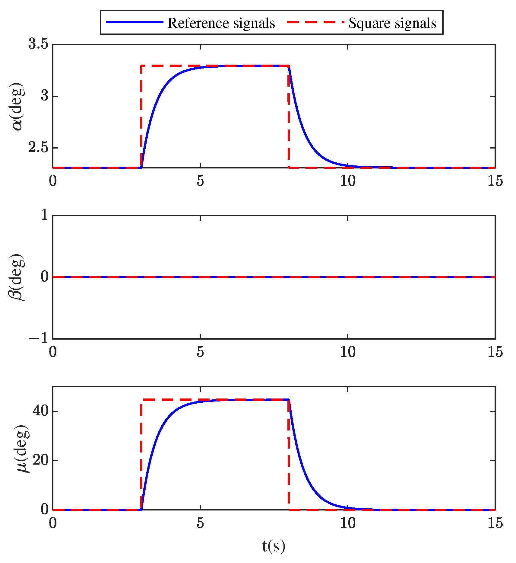
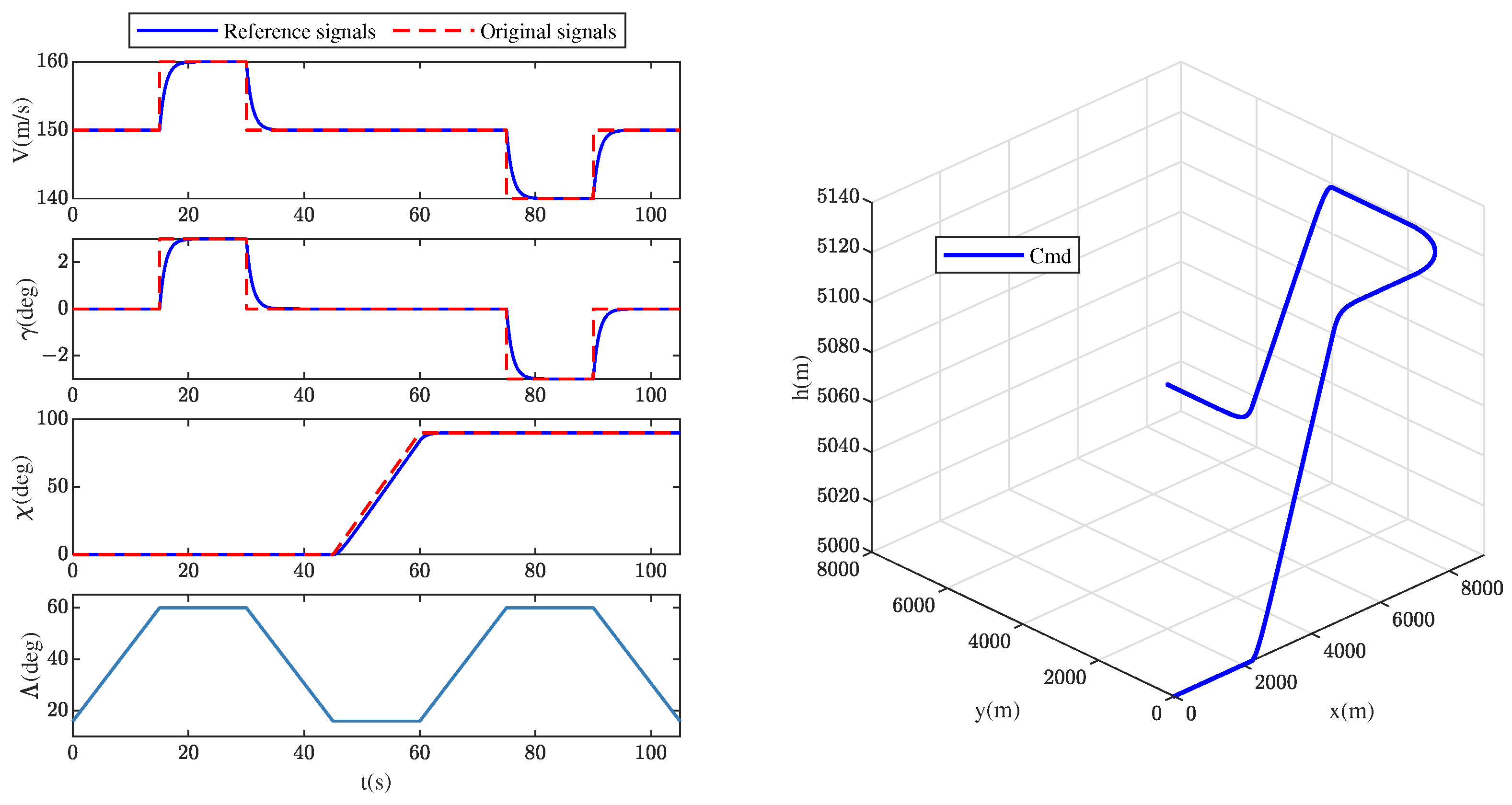
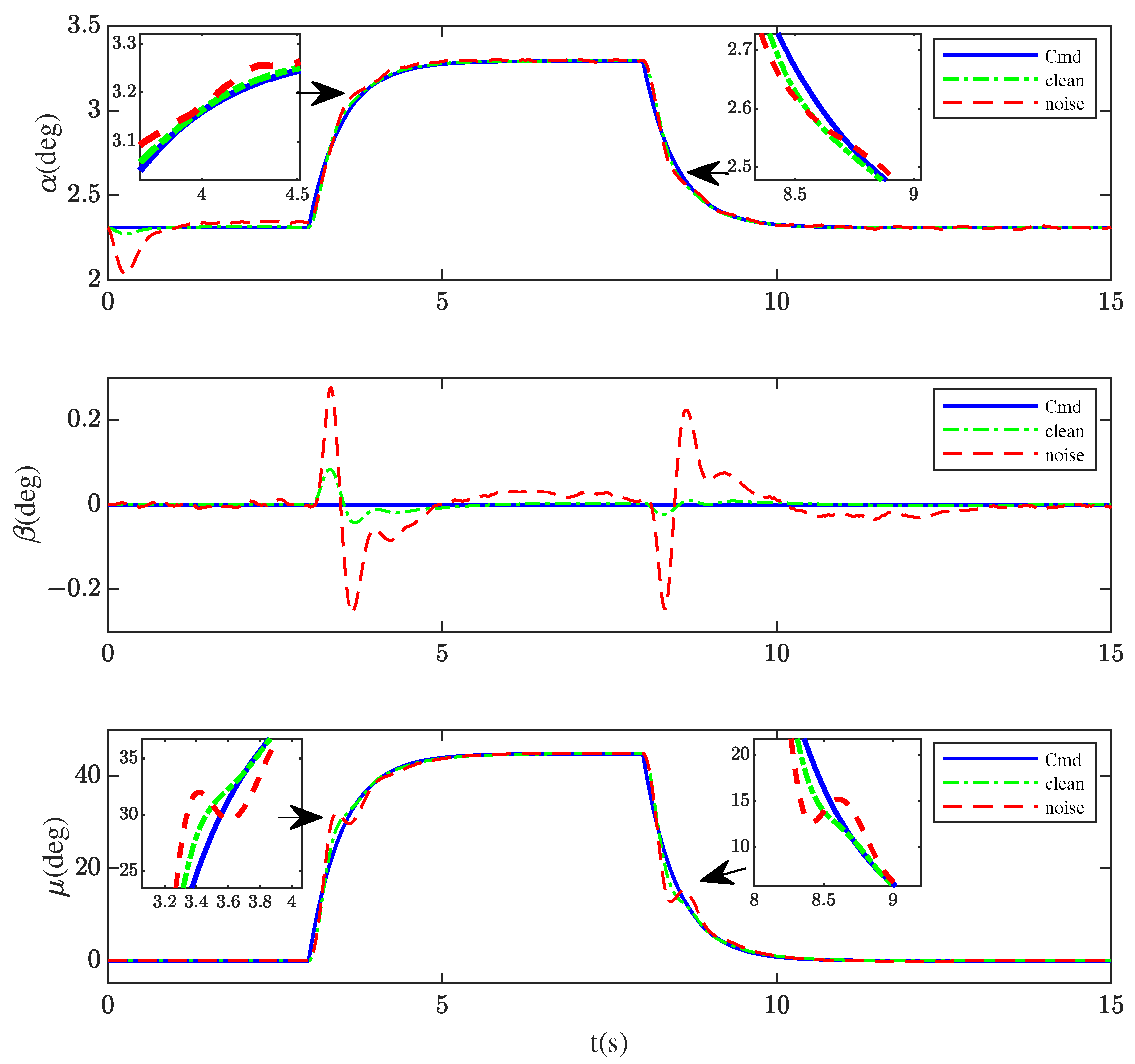
The initial condition of the simulation is horizontal cruise ($V_0$ = 150 m/s, $H_0$ = 5000 m, ${\alpha }_0$ = ${2.309}^{\circ }$, ${\beta }_0={\mu }_0$ = $0^{\circ }$). The wings of the aircraft started to sweep symmetrically from ${15.97}^{\circ }$ at the time of t = 0 s and reached a maximum sweep angle of ${60}^{\circ }$ at t = 15 s. While the shape was changing, the aircraft was required to keep the initial horizontal flight for 3 s. Then, the step commands of ${\alpha }_c$ = ${3.294}^{\circ }$ and ${\mu }_c$ = ${45}^{\circ }$ were given to realize the roll maneuver. Further, at t = 8 s, the angle of attack $\alpha$ and bank angle $\mu$ were allowed to return back to their initial values. The expected value of $\beta$ was always 0. All the commands mentioned above would pass through a filter and the reference signals are shown in the Figure 7.

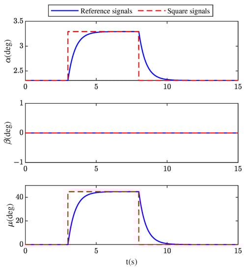
Figure 7. Command signals in Scenario 1.

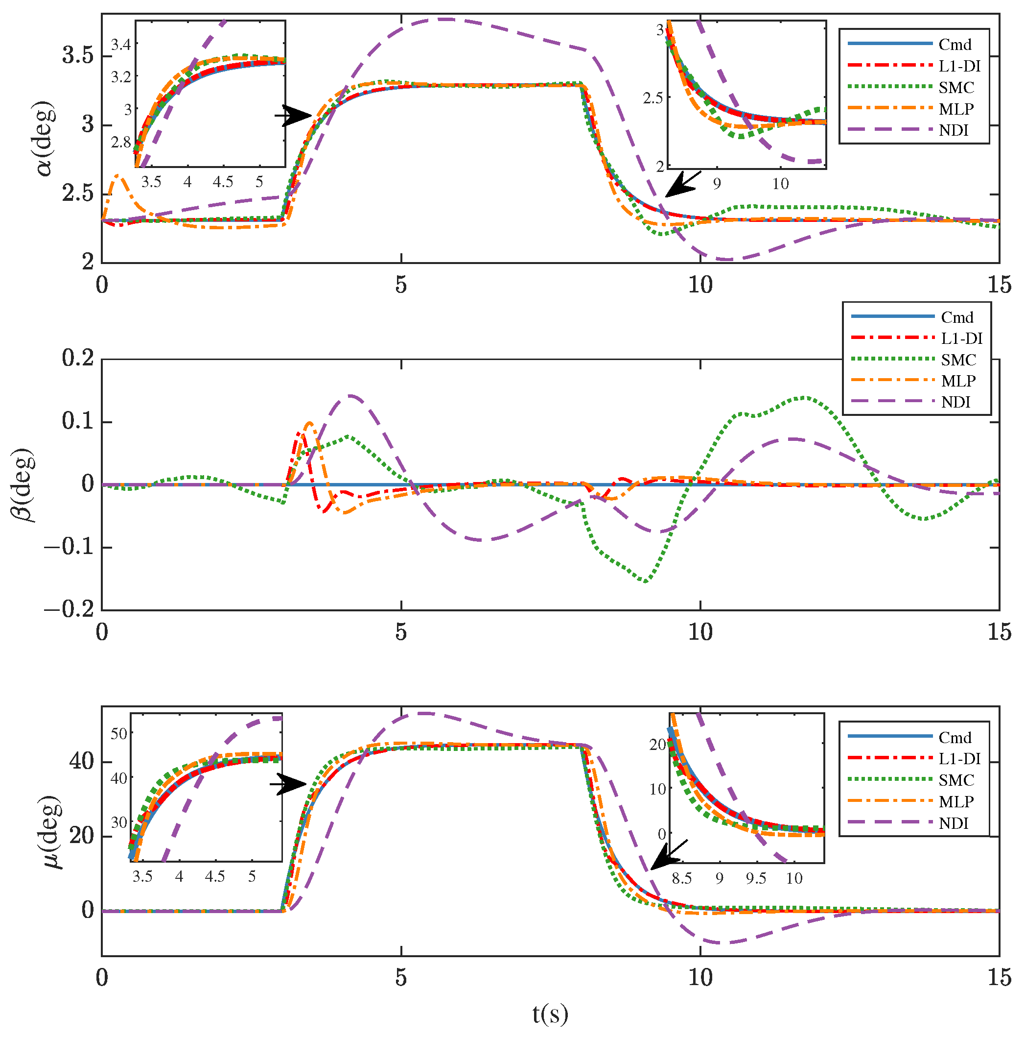
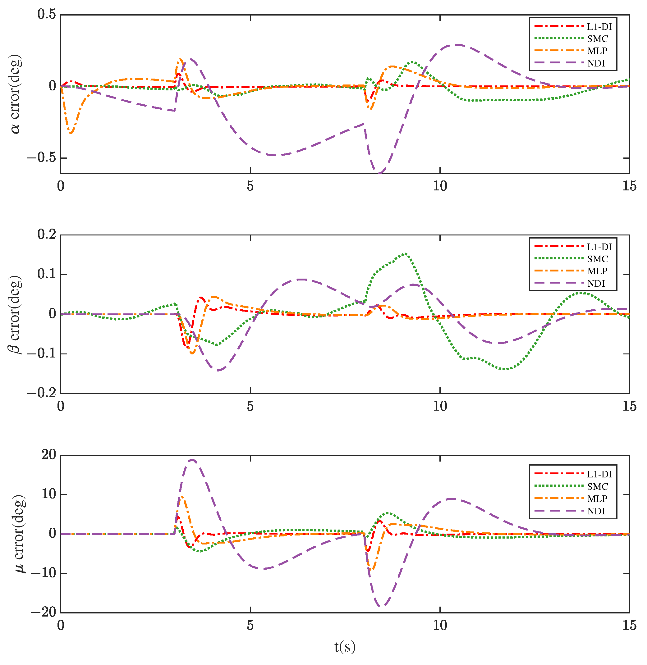
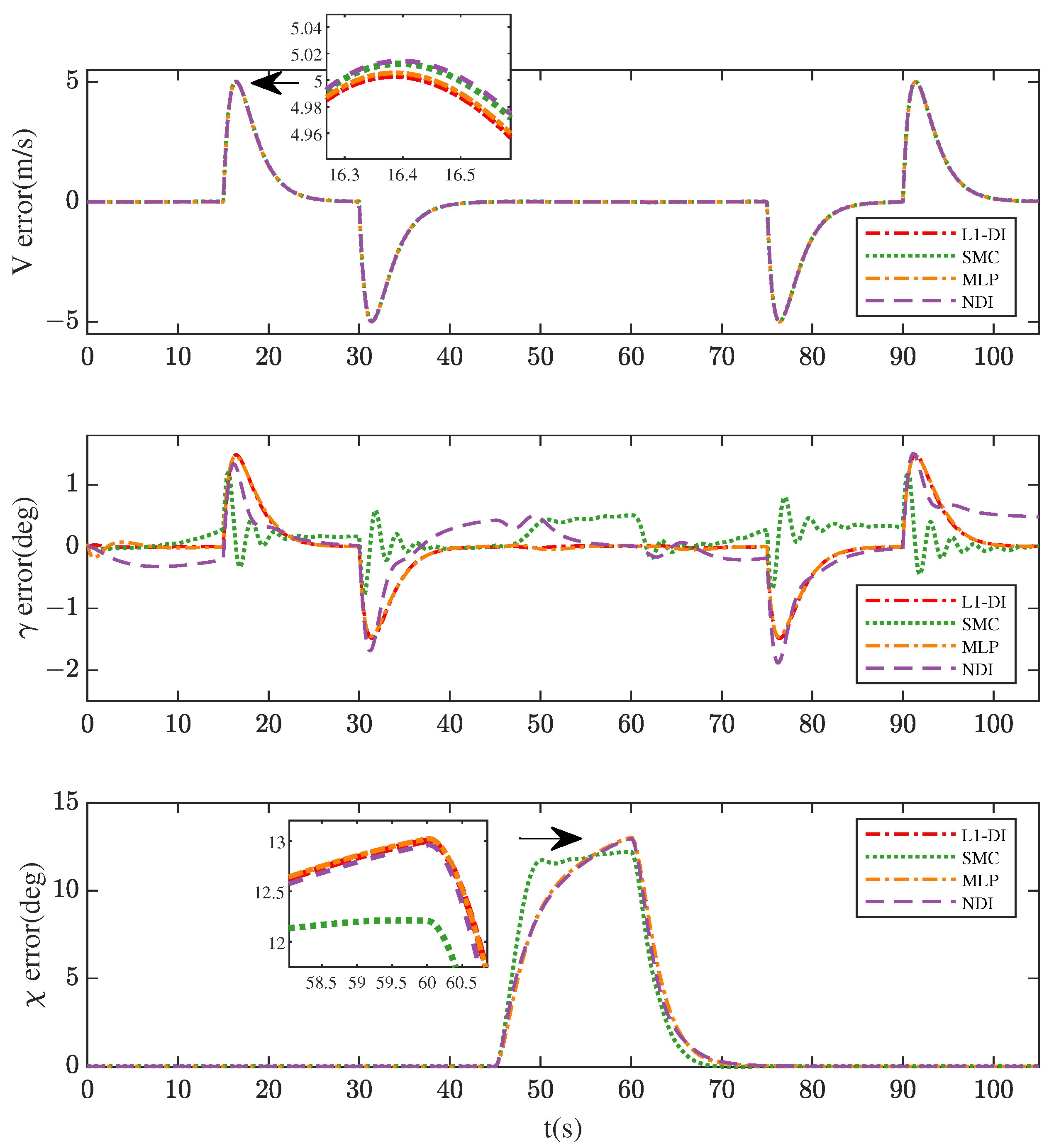
Figure 8, Figure 9 and Figure 10 show the command tracking performance of different control methods in Scenario 1. During $t\in [0s,3s]$, due to the shape of the aircraft starting to change from t = 0 s, CG movement and parameter variations make it difficult for the aircraft to remain stable. Compared to SMC, ${\mathcal{L}}_1$-DI and MLP exhibit a distinct state change at the beginning, especially MLP, for they have an adaptive process to model variation at the beginning. However, the tracking error of MLP is much higher than that of ${\mathcal{L}}_1$-DI during this period, which means the adaptive speed of the neural network is slower. Furthermore, the tracking error of ${\mathcal{L}}_1$-DI reduces to the minimum rapidly before t = 3 s and, contrarily, that of NDI increases steadily, for it is generally sensitive to model variation during the morphing phase and may not provide robustness against such uncertainties.

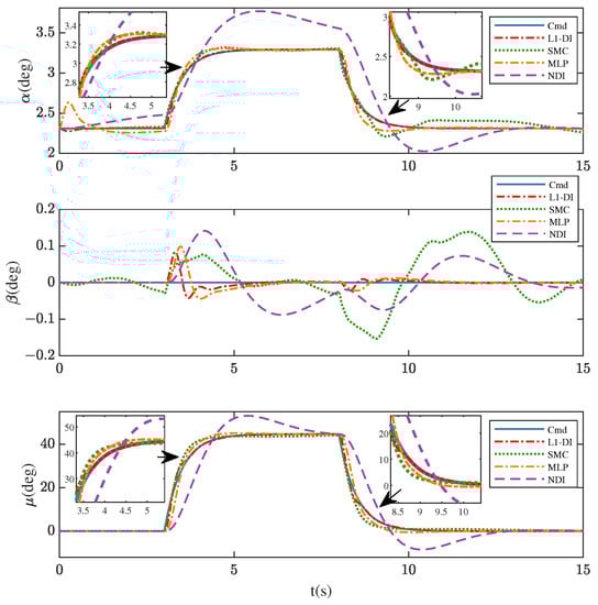
Figure 8. Command signals tracking of $\alpha$, $\beta$, and $\mu$ in Scenario 1.

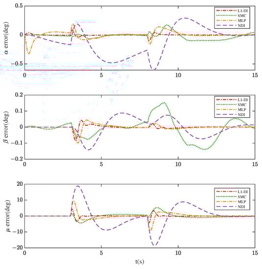
Figure 9. Tracking error of $\alpha$, $\beta$, and $\mu$ in Scenario 1.

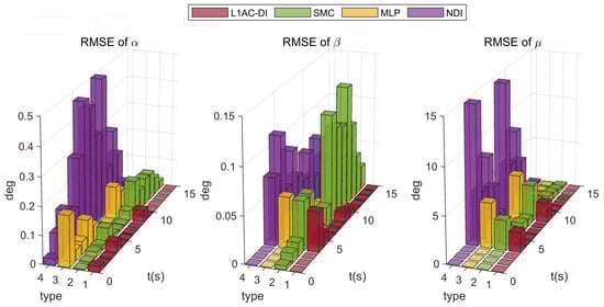
Figure 10. RMSE for different control methods.

When the maneuver commands are given at $t=3$ s, the tracking error of each controller begins to increase, especially NDI. However, ${\mathcal{L}}_1$-DI can cope with such a situation and always follows the reference command closely. The control performance indicators like overshoot and the tracking accuracy of ${\mathcal{L}}_1$-DI are obviously superior to those of the other controllers. At the time $t>8$ s, the attitude angles are supposed to turn back to the initial values, and the state responses under ${\mathcal{L}}_1$-DI can follow the commands quickly and accurately. Finally, after $t>10$ s, the steady-state errors of ${\mathcal{L}}_1$-DI are minimal (as shown in Figure 10), followed by MLP, SMC, and NDI.

Figure 10 demonstrates the root mean square errors (RMSE) of different controllers during simulations, the value of each box represents the average value of square errors at each time interval (1 s) and it shall be calculated by the formula below:

$$\sqrt{\frac{{\sum }_{i=1}^{\frac{1}{\Delta t}}{e}_{n_i}^2}{\frac{1}{\Delta t}}},$$

(109)

where $\Delta t=0.001$ s is the simulation step size and $n=0,1,2,\cdots ,14$ represent the beginning of fifteen time intervals. $e_{n_i}$ represents the tracking error calculated by the ith step during n to $n+1$ s.

To help to compare the controller performance, the tracking errors of each controller were evaluated and summarized in Table 3 including minimal errors, max errors, and RMSE ($\sqrt{\frac{{\sum }_{j=1}^{\frac{15}{\Delta t}}{e}_j^2}{\frac{15}{\Delta t}}}$) throughout the overall simulation period (mark the values less than $1\times {10}^{-5}$ as 0). Results indicate that all controllers have guaranteed tracking performance and ${\mathcal{L}}_1$-DI achieves the best, for its minimal values of all types of error.

Table 3. Error information of different controllers.

Time (s)	V (m/s)			$\mathit{\gamma }$ (deg)			$\mathit{\chi }$ (deg)
	min	max	RMSE	min	max	RMSE	min	max	RMSE
${\mathcal{L}}_1$-DI	0	0.0993	0.0157	0	0.0844	0.0122	0	4.2945	0.7734
SMC	$1.2754\times {10}^{-5}$	0.1710	0.0565	0	0.1536	0.0650	0	5.2775	1.4959
MLP	0	0.3247	0.0686	0	0.0986	0.0168	0	9.3999	1.9038
NDI	0	0.6070	0.2602	0	0.1415	0.0536	0	18.8475	6.6398

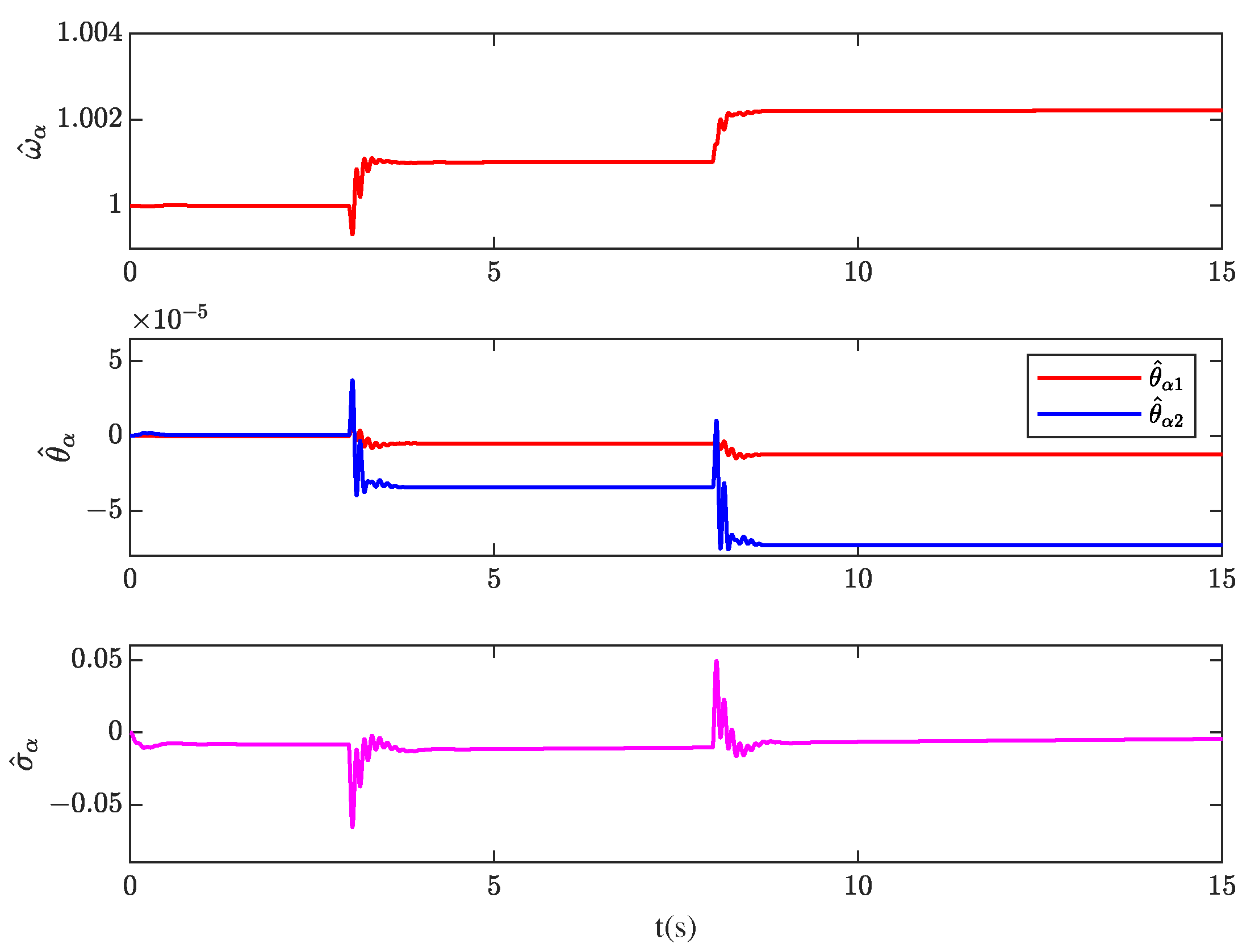
In addition, Figure 11 shows the change of the estimate of parameters ${\widehat{\omega }}_{\alpha }$, ${\widehat{\mathit{\theta }}}_{\alpha }$, and ${\widehat{\sigma }}_{\alpha }$ in the ${\mathcal{L}}_1$ adaptive controller. Here, the parameters of the $\alpha$ channel are taken as an example:

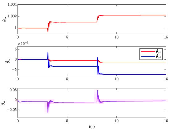
Figure 11. The estimate of parameters ${\widehat{\omega }}_{\alpha }$, ${\widehat{\mathit{\theta }}}_{\alpha }$, and ${\widehat{\sigma }}_{\alpha }$.

The results indicate that the estimated parameters governed by the adaptive law in Section 4.3 are capable of adjusting their values adaptively according to the tracking error and then the ${\mathcal{L}}_1$ adaptive controller can generate the control law immediately and autonomously to ensure stable reference tracking.

6.1.2. Scenario 2

To help evaluate different strategies under varied circumstances, we designed an enriched test scenario covering a wide range of situations and conditions, which included cruise, expedite climbing, coordinated turning, and diving. Meanwhile, shape variation instructions were given during the flight. The above maneuvers were performed by tracking the following flight path command of V, $\gamma$, and $\chi$, which passed through filters and are given in Table 4 and Figure 12.

Table 4. Command signals given in Scenario 3.

Times (s)	V (m/s)	$\mathit{\gamma }$ (deg)	$\mathit{\chi }$ (deg)	Sweep Angle (deg)
0∼15	150	0	0	15.97∼60
15∼30	160	3	0	60
30∼45	150	0	0	60∼15.97
45∼60	150	0	0∼90	15.97
60∼75	150	0	90	15.97∼60
75∼90	140	−3	90	60
90∼105	150	0	90	60∼15.97

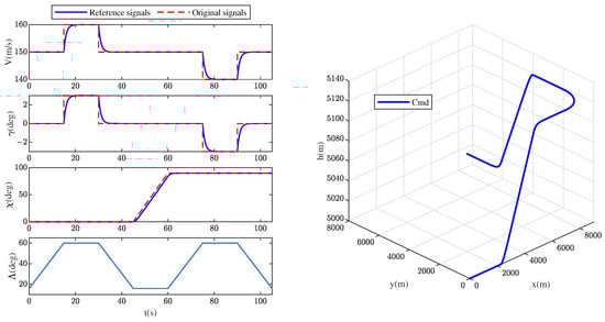
Figure 12. Command signals and ideal flight trajectory in Scenario 2.

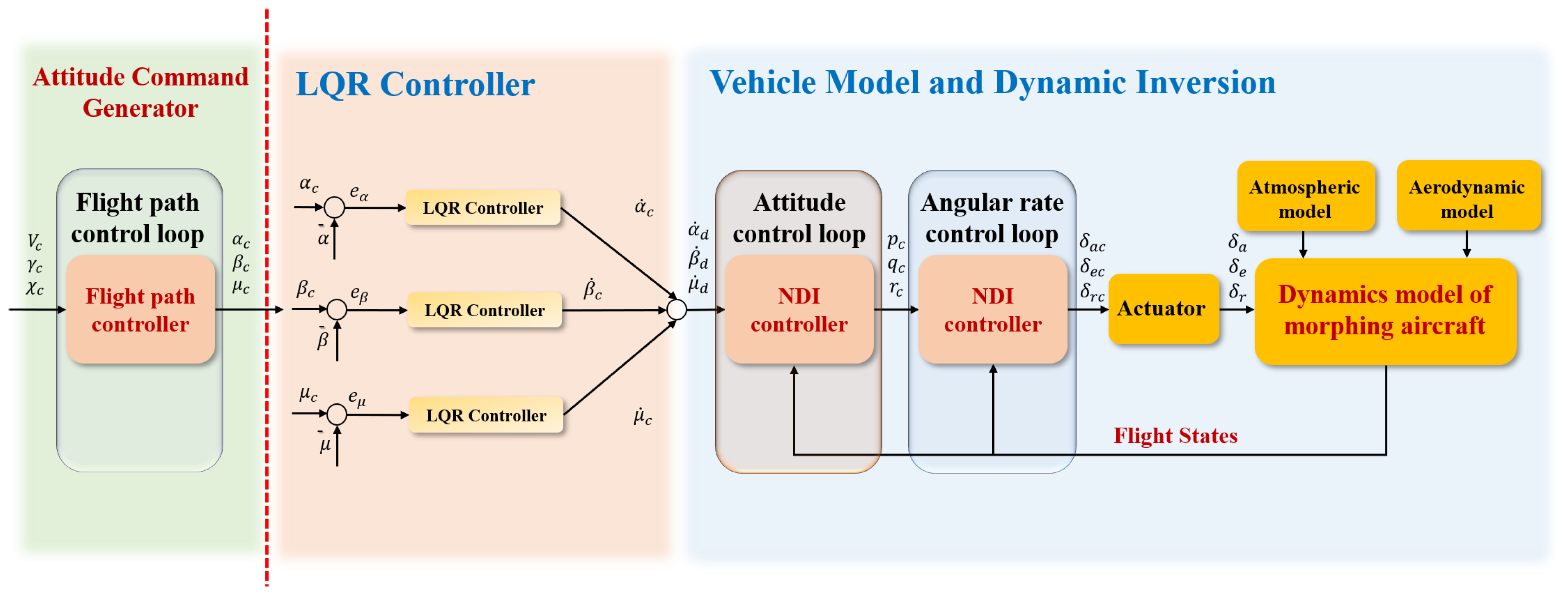
It should be noted that the control approach proposed in this paper is aimed at vehicle attitude control, which cannot realize flight path control. In order to realize the flight path command tracking and verify the effectiveness of the presented controller after incorporating a complete flight control system, a flight path control loop was designed and then replaced the command signals generator in Figure 6 to calculate the expected ${\alpha }_c$, ${\beta }_c$, and ${\mu }_c$ as the input of the attitude controller according to the flight path command of $V_c$, ${\gamma }_c$, and ${\chi }_c$. The same flight path control loop was added to the outermost loop of the controllers based on ${\mathcal{L}}_1$-DI, SMC, MLP, and NDI. The the development of the flight path control loop has been given in [29,39] in detail. The overall architecture of ${\mathcal{L}}_1$-DI, SMC, MLP, and NDI after adding the flight path controller are demonstrated in Appendix B.

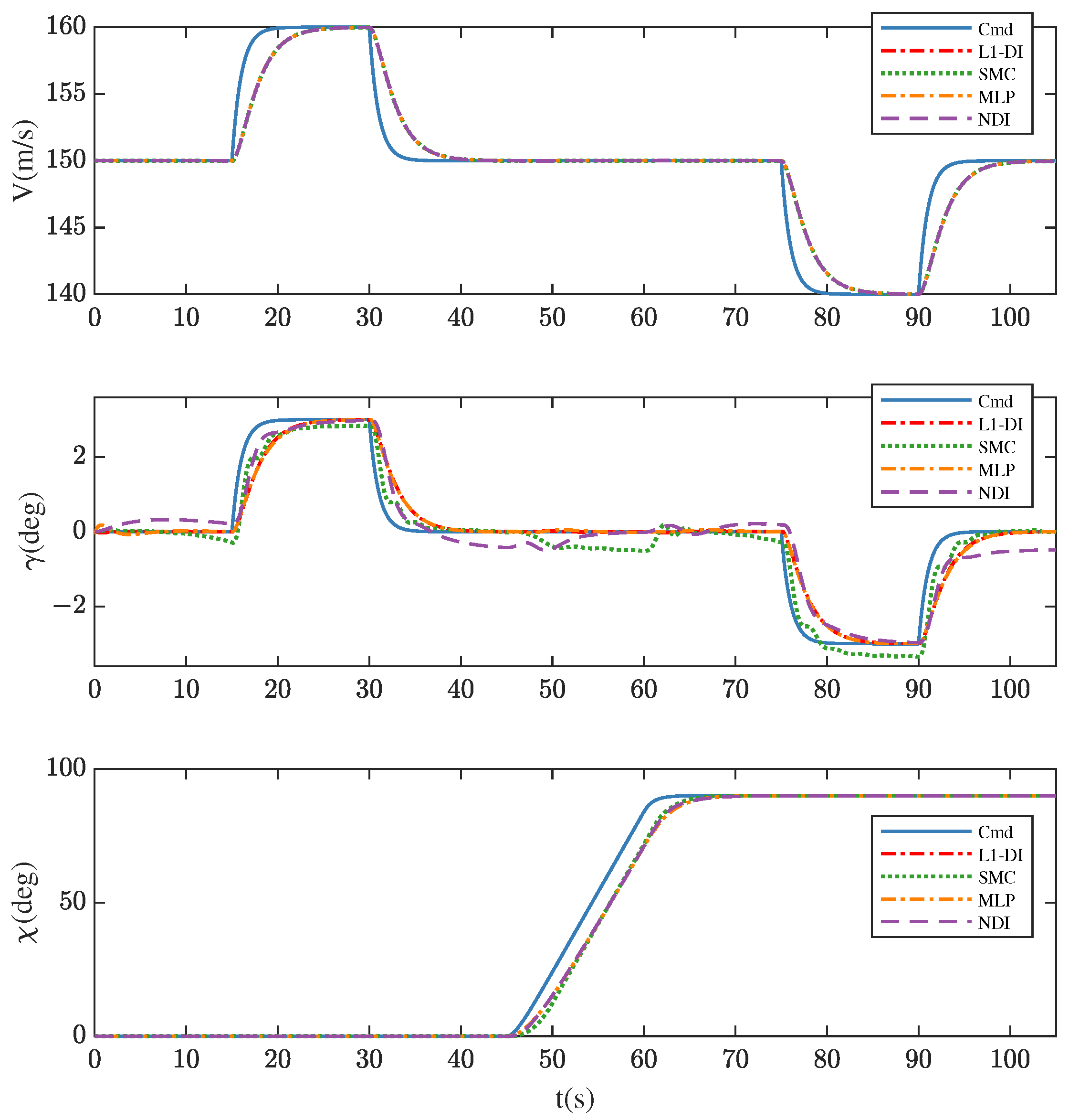
Figure 13 and Figure 14 show the V, $\gamma$, and $\chi$ commands and responses for different controllers. The results demonstrate that the tracking performances of different controllers are slightly different, which is caused by the distinct attitude control strategies employed by the inner layer. This indicates the importance of designing an effective attitude controller to realize the desired attitude responses. Specifically, in V and $\chi$ channels, there is little difference in tracking performance between the four controllers. However, in the $\gamma$ channel, SMC shows performance degeneration in the $\gamma$ channel for steady-state error, and the buffeting effect is always present; consistent with the results in Scenario 1, NDI has the worst tracking performance in the morphing phase (during 0∼15 s, 30∼45 s, 60∼75 s and 90∼105 s) with the highest tracking error and a poor convergence performance.

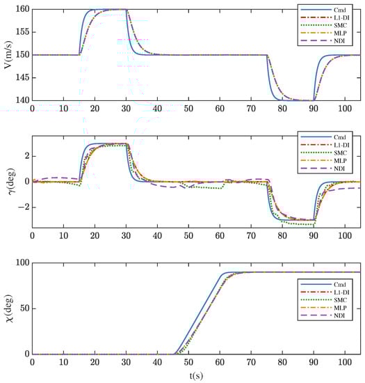
Figure 13. Command signals tracking of V, $\gamma$, and $\chi$ in Scenario 2.

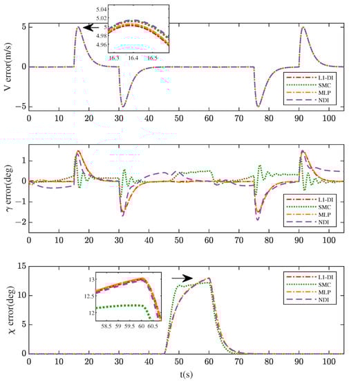
Figure 14. Tracking errors of V, $\gamma$, and $\chi$ in Scenario 2.

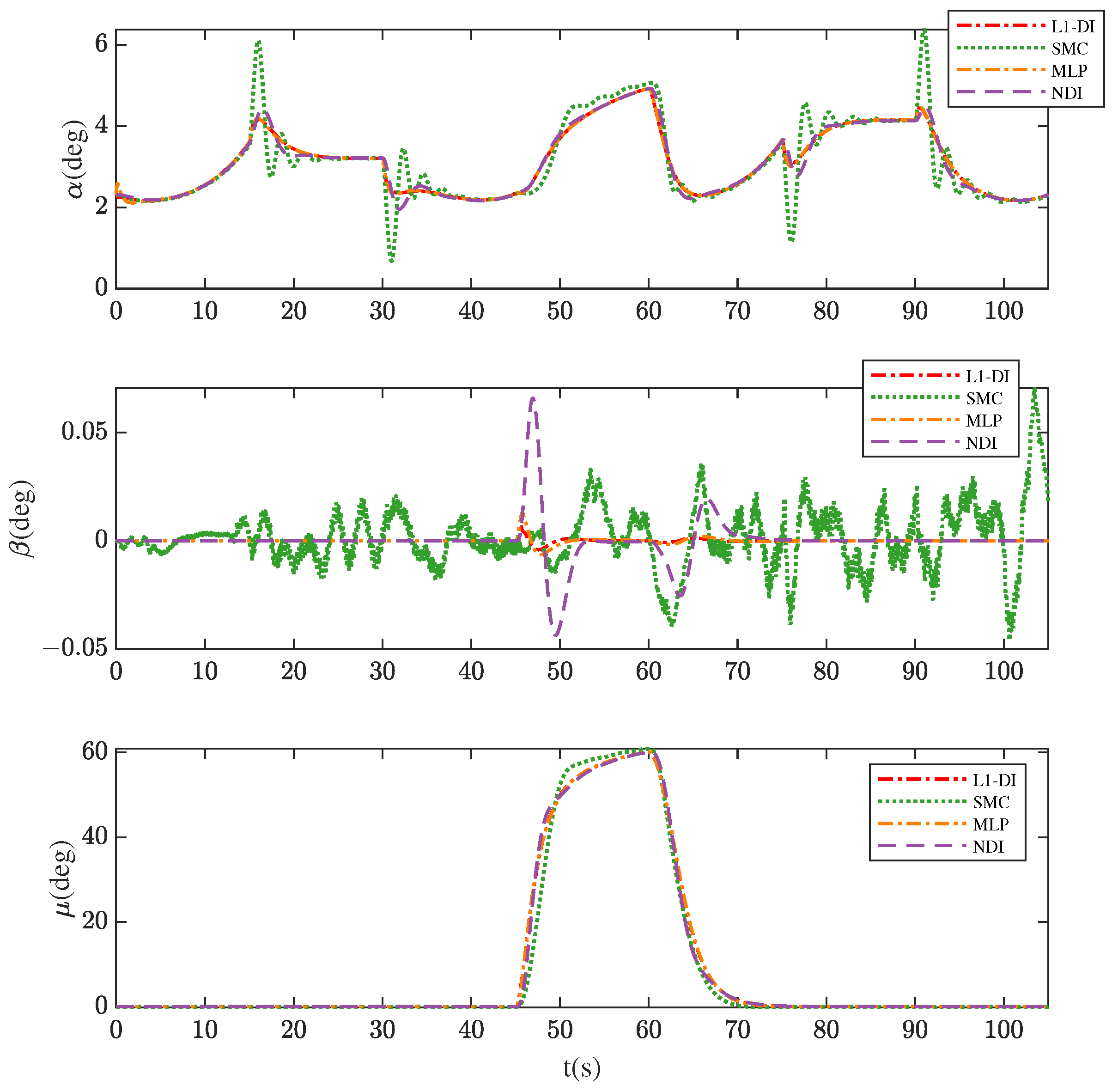
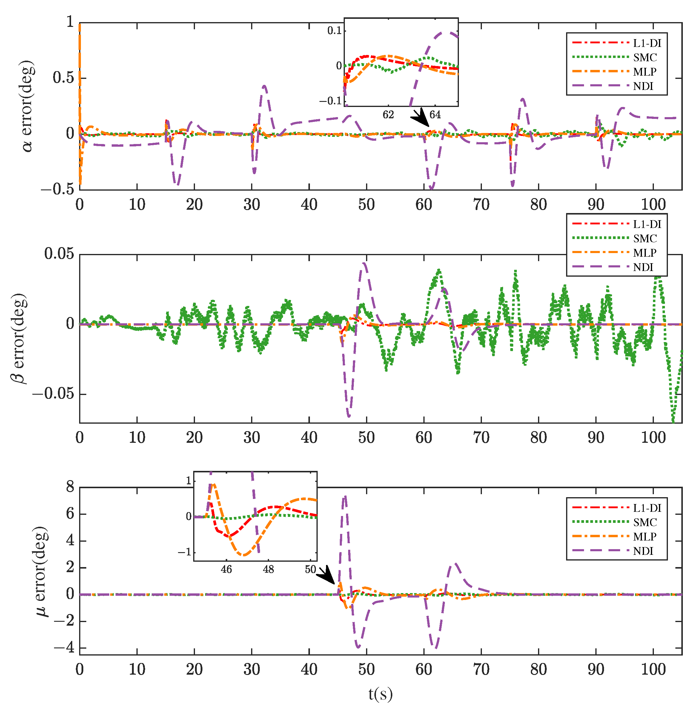
Figure 15 and Figure 16 show the responses of $\alpha$, $\beta$, and $\mu$ and the tracking errors of the responses. The results demonstrate that ${\mathcal{L}}_1$-DI, MLP, and NDI are able to maintain a relatively stable state response and ${\mathcal{L}}_1$-DI achieves the best tracking performance of the three. SMC performs the best tracking performance in the $\mu$ channel (the tracking error of SMC shown in Figure 16 is the smallest). However, in $\alpha$ and $\beta$ channels, the responses of SMC exhibit more unpleasant jitters and chattering behavior compared to other three controllers, as the ideal sliding mode implies an infinite switching frequency; however, this cannot be attained in practice [40], which means the actual system states cannot reach the predefined sliding surface. Overall, ${\mathcal{L}}_1$-DI yields satisfactory results in the flight control system architecture, for it maintains a stable state response with smaller tracking errors.

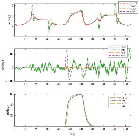
Figure 15. Command signals tracking of $\alpha$, $\beta$, and $\mu$ in Scenario 2.

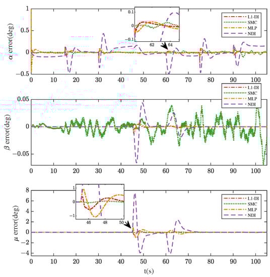
Figure 16. Tracking errors of $\alpha$, $\beta$, and $\mu$ in Scenario 2.

The overall flight trajectories of the four controllers are shown in Figure A5.

6.2. Sensitivity Analysis

To illustrate the good robustness and performance of the proposed controller in some other cases, the same attitude commands in Scenario 1 were given in the following scenarios:

• In Scenario 3, the uncertainties were introduced, which included sensor measurement errors and control surface disturbances, shown in Table 5.
  Table 5. The type and range of uncertainties.

  States	Measurement Error Range
  V	$[-0.5\mathrm{m}/\mathrm{s},0.5\mathrm{m}/\mathrm{s}]$
  $\alpha ,\beta$	$\left[-{0.2}^{\circ },{0.2}^{\circ }\right]$
  $p,q,r$	$\left[-{0.15}^{\circ }/\mathrm{s},{0.15}^{\circ }/\mathrm{s}\right]$
  $\varphi ,\mathit{\theta },\psi$	$\left[-{1.5}^{\circ },{1.5}^{\circ }\right]$
  ${\delta }_a,{\delta }_e,{\delta }_r$	$[-10\%,10\%]$

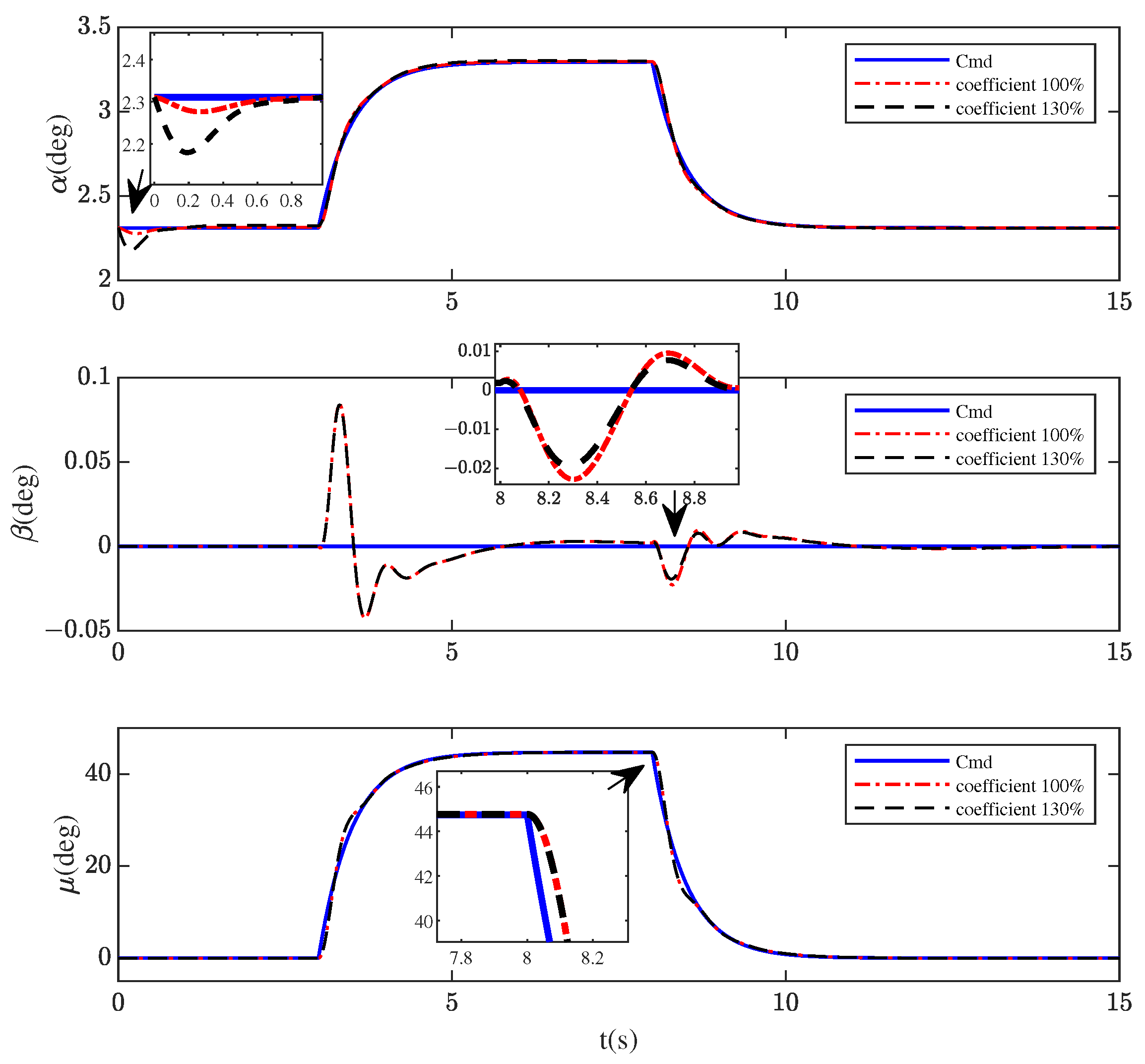
• In Scenario 4, aiming at the model uncertainties, aerodynamic coefficient perturbation was considered, and aerodynamic forces and moments coefficients were increased by 30% to check if the controller can still achieve a satisfactory performance.
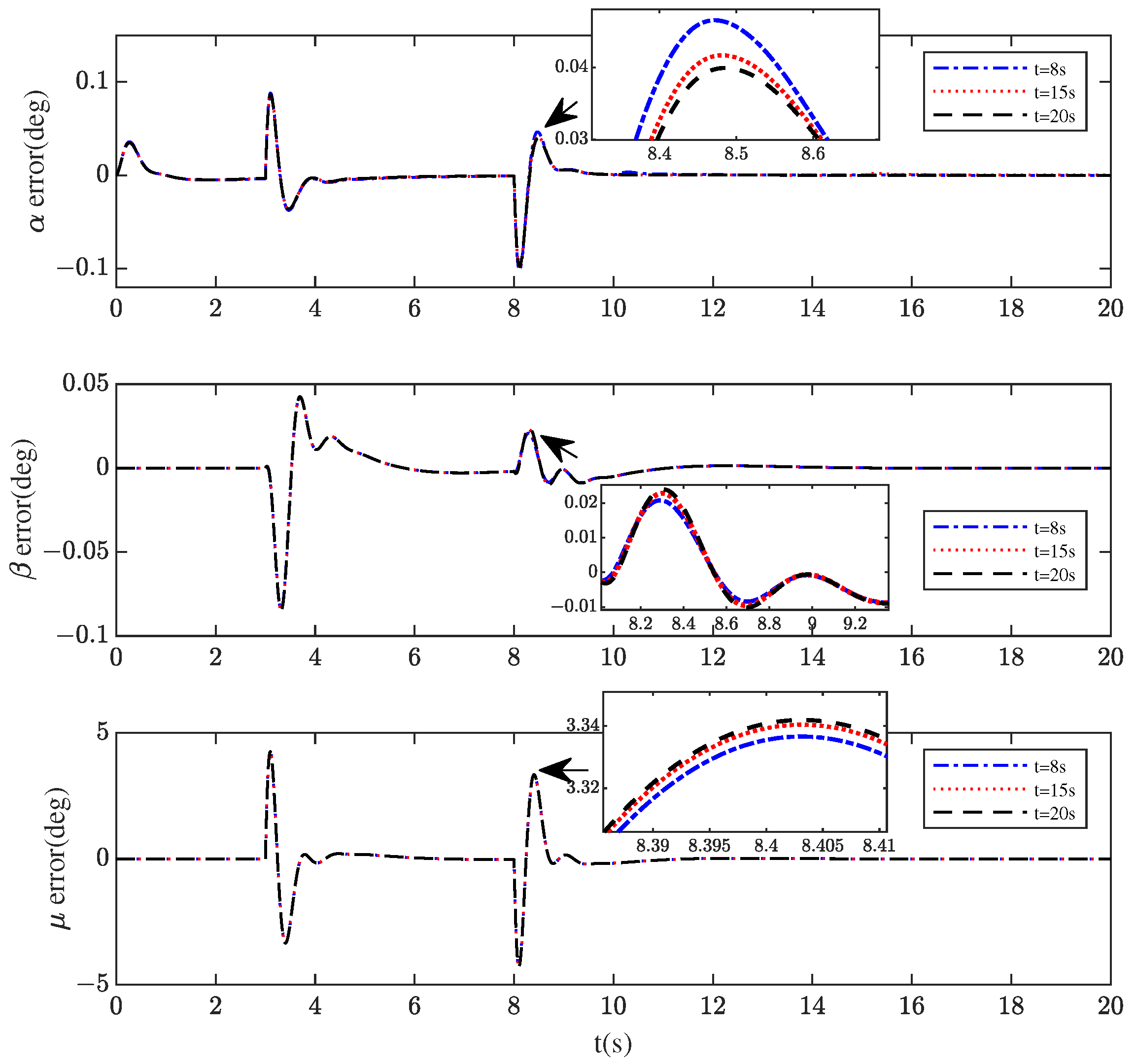
• In Scenario 5, the morphing rates were changed and the aircraft was allowed to change from the loiter configuration ($\Lambda ={15.97}^{\circ }$) to the dash configuration in 8 s, 15 s, and 20 s to observe whether the control performance was affected.

Figure 17, Figure 18 and Figure 19 show the control performance of the proposed scheme in three situations. Figure 17 illustrates that the ${\mathcal{L}}_1$-DI controller can offset the deviation caused by uncertainties to guarantee the low command tracking errors and the convergence within an acceptable range. Figure 18 and Figure 19 show very consistent performances for increased aerodynamic forces and moments and different shape variation speeds. The influence in Scenarios 4 and 5 is almost negligible.

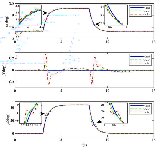
Figure 17. Signal tracking of $\alpha$, $\beta$, and $\mu$ in Scenario 3.

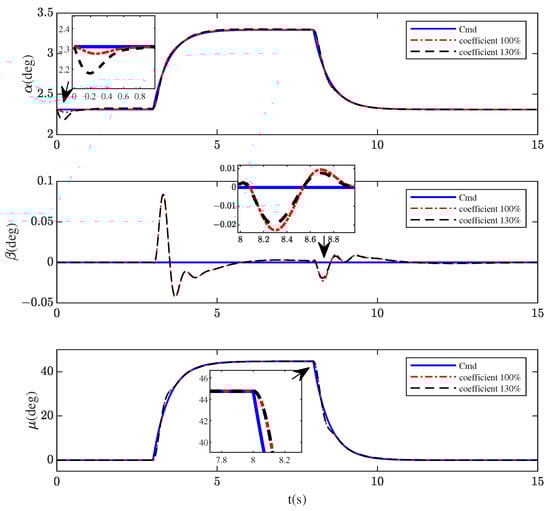
Figure 18. Signal tracking of $\alpha$, $\beta$, and $\mu$ in Scenario 4.

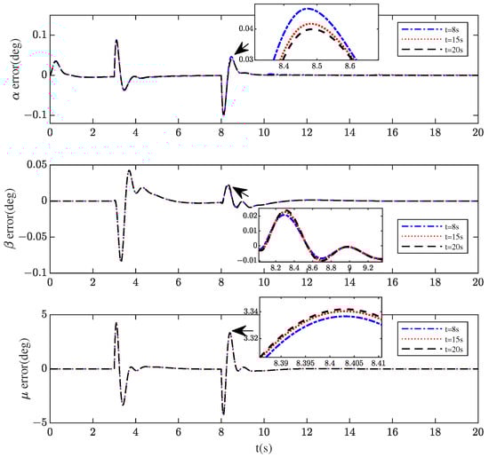
Figure 19. Tracking error of $\alpha$, $\beta$, and $\mu$ in Scenario 5.

The simulation results in Scenarios 1 and 2 indicate that the control approach based on ${\mathcal{L}}_1$ adaptive control and dynamic inversion has improved the performance in the presence of shape change compared to that of other well-known controllers. Additionally, in Scenarios 3–5, the robustness of the controller to external disturbances and model uncertainties is satisfactory.

7. Conclusions

An implementation of a ${\mathcal{L}}_1$ adaptive controller based on dynamic inversion has been presented and demonstrated with a validated simulation of a variable-sweep morphing aircraft. Results show that the proposed control method has a more satisfactory command tracking performance compared to that of other popular controllers. While tracking the maneuver commands in Scenario 1, the maximum tracking error and the RMSE of ${\mathcal{L}}_1$-DI in the $\alpha$ channel are ${0.0993}^{\circ }$ and ${0.0157}^{\circ }$, respectively, followed by an SMC with a maximum tracking error and RMSE of ${0.1710}^{\circ }$ and ${0.0565}^{\circ }$, respectively. In the $\beta$ and $\mu$ channels, ${\mathcal{L}}_1$-DI also achieves the best control performance, as the maximum error and RMSE of the former are ${0.0844}^{\circ }$ and ${0.0122}^{\circ }$, followed by ${0.0986}^{\circ }$ and ${0.0168}^{\circ }$, respectively, while those of the latter are ${4.2945}^{\circ }$ and ${0.7734}^{\circ }$, followed by ${5.2775}^{\circ }$ and ${1.4959}^{\circ }$, respectively. In Scenario 2, the effectiveness of the proposed controller after adding a flight path control loop has been verified. As an attitude controller in the inner loop, ${\mathcal{L}}_1$-DI has a smaller tracking error, a smaller overshoot, and a more satisfactory convergence performance in $\alpha$, $\beta$, and $\mu$ channels than those of MLP and NDI, and, compared to SMC, it yields guaranteed stable responses of $\alpha$, $\beta$, and $\mu$. Finally, a sensitivity analysis of Scenarios 3–5 has proven the strong robustness of the controller to uncertainties. The control scheme proposed in this paper is feasible and effective. In the future, physical verification can be carried out on the basis of simulation to prove that the proposed scheme has practical value.

Appendix B.1

This appendix contains the structure of ${\mathcal{L}}_1$-DI, SMC, MLP, and NDI controller to help understand how to develop this controllers.

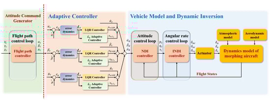
Figure A1. Schematic of the proposed ${\mathcal{L}}_1$-DI method.

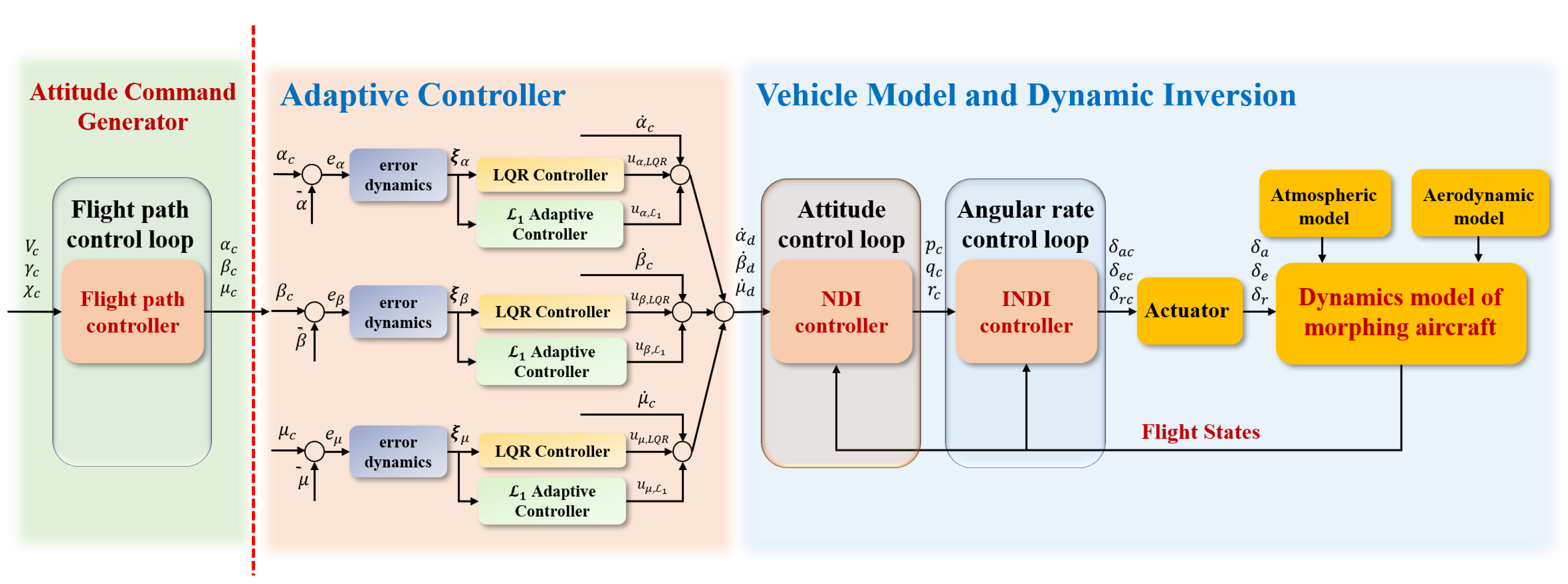
Figure A2. Schematic of the SMC control method.

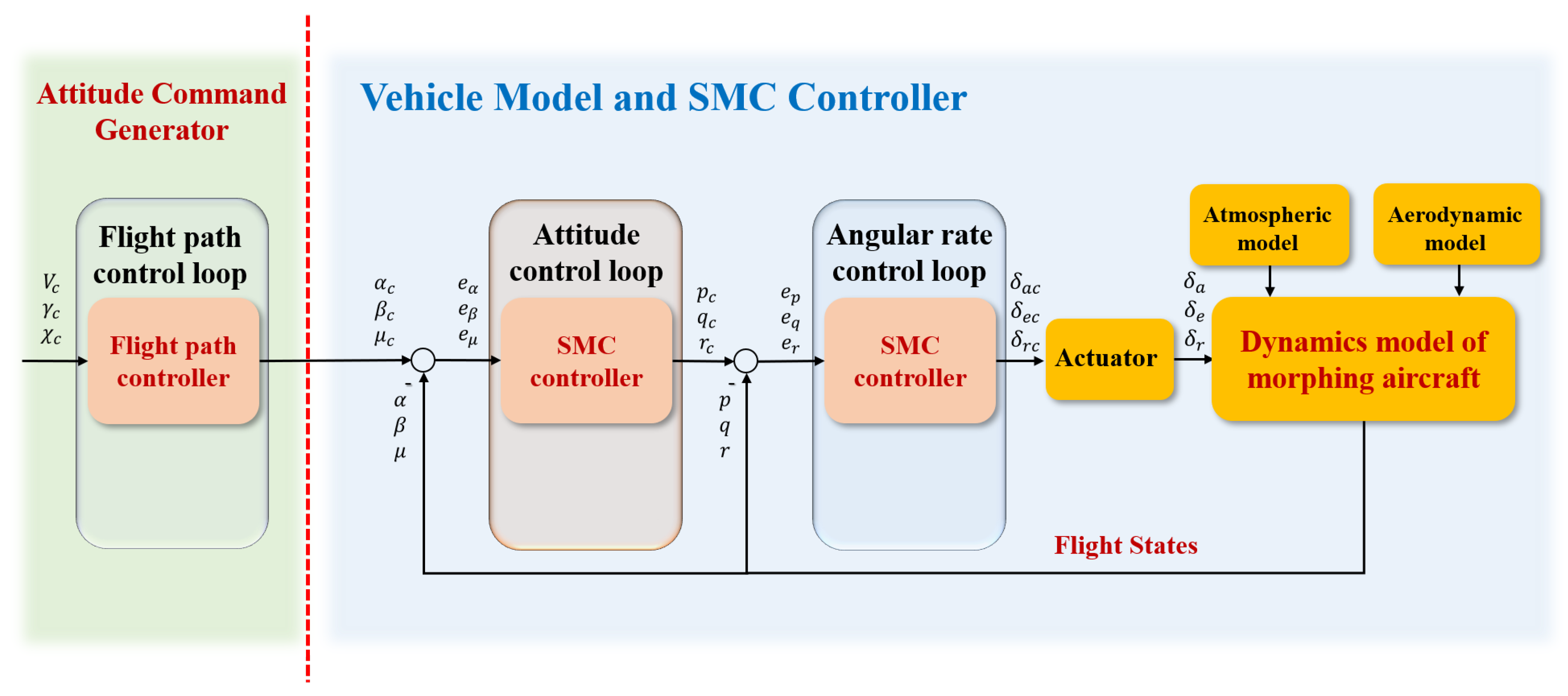
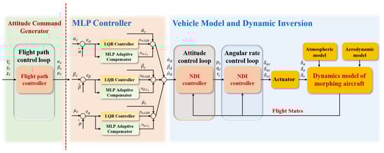
Figure A3. Schematic of the MLP method.

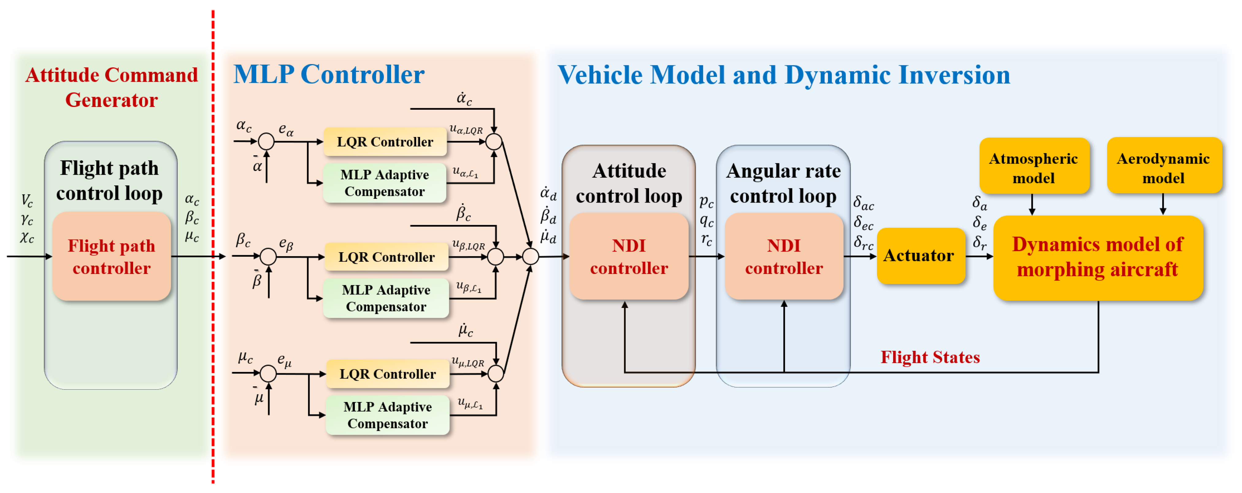
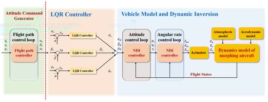
Figure A4. Schematic of the NDI method.

Appendix B.2

The flight trajectories of the four controllers are shown in Figure A5.

Figure A5. The flight trajectory of different controllers.

References

- Yue, T.; Zhang, X.; Wang, L.; Ai, J. Flight dynamic modeling and control for a telescopic wing morphing aircraft via asymmetric wing morphing. Aerosp. Sci. Technol. 2017, 70, 328–338. [Google Scholar] [CrossRef]
- Xu, W.; Li, Y.; Pei, B.; Yu, Z. Coordinated intelligent control of the flight control system and shape change of variable sweep morphing aircraft based on dueling-DQN. Aerosp. Sci. Technol. 2022, 130, 107898. [Google Scholar] [CrossRef]
- Barbarino, S.; Bilgen, O.; Ajaj, R.M.; Friswell, M.I.; Inman, D.J. A review of morphing aircraft. J. Intell. Mater. Syst. Struct. 2011, 22, 823–877. [Google Scholar] [CrossRef]
- Yue, T.; Wang, L.; Ai, J. Gain self-scheduled H∞ control for morphing aircraft in the wing transition process based on an LPV model. Chin. J. Aeronaut. 2013, 26, 909–917. [Google Scholar] [CrossRef]
- Li, Y.; Liu, X.; He, Q.; Ming, R.; Huang, W.; Zhang, W. Adaptive Structure-Based Nonlinear Dynamic Inversion Control for Aircraft with Center of Gravity Variations. J. Intell. Robot. Syst. 2022, 106, 4. [Google Scholar] [CrossRef]
- Wang, Q.; Wang, T.; Hou, D.; Dong, C. Robust LPV control for morphing vehicles via velocity-based linearization. J. Syst. Eng. Electron. 2014, 36, 1130–1136. [Google Scholar]
- Lu, B.; Wu, F. Switching LPV control designs using multiple parameter-dependent Lyapunov functions. Automatica 2004, 40, 1973–1980. [Google Scholar] [CrossRef]
- Cheng, H.; Chaoyang, D.; Jiang, W.; Qing, W.; Yanze, H. Non-fragile switched H∞ control for morphing aircraft with asynchronous switching. Chin. J. Aeronaut. 2017, 30, 1127–1139. [Google Scholar] [CrossRef]
- Jiang, W.; Wu, K.; Wang, Z.; Wang, Y. Gain-scheduled control for morphing aircraft via switching polytopic linear parameter-varying systems. Aerosp. Sci. Technol. 2020, 107, 106242. [Google Scholar] [CrossRef]
- Xu, W.; Li, Y.; Lv, M.; Pei, B. Modeling and switching adaptive control for nonlinear morphing aircraft considering actuator dynamics. Aerosp. Sci. Technol. 2022, 122, 107349. [Google Scholar] [CrossRef]
- Wei, C.; Jingchao, L.; Xiaoguang, W.; Weiguo, Z. Design of a controller for morphing aircraft based on backstepping/RHO. J. B. Univ. Aeronaut. Astronaut. Univ. Aeronaut. Astronaut. 2014, 40, 1060–1065. [Google Scholar]
- Yuan, L.; Wang, L.; Xu, J. Adaptive fault-tolerant controller for morphing aircraft based on the L2 gain and a neural network. Aerosp. Sci. Technol. 2023, 132, 107985. [Google Scholar] [CrossRef]
- Qiao, F.; Shi, J.; Zhang, W.; Lyu, Y.; Qu, X. A high precision adaptive back-stepping control method for morphing aircraft based on RBFNN method. J. Northwest. Polytechnical. Univ. 2020, 38, 540–549. [Google Scholar] [CrossRef]
- Qiao, F.; Zhang, W.; Li, G.; Shi, J.; Qu, X.; Che, J.; Zhou, H. Robust Adaptive Back-stepping Control Design Based on RBFNN for Morphing Aircraft. In Proceedings of the 2018 IEEE CSAA Guidance, Navigation and Control Conference (CGNCC), Xiamen, China, 10–12 August 2018; pp. 1–7. [Google Scholar]
- Horn, J.F. Non-linear dynamic inversion control design for rotorcraft. Aerospace 2019, 6, 38. [Google Scholar] [CrossRef]
- Sieberling, S.; Chu, Q.; Mulder, J. Robust flight control using incremental nonlinear dynamic inversion and angular acceleration prediction. J. Guid. Control. Dynam. 2010, 33, 1732–1742. [Google Scholar] [CrossRef]
- Zhou, C.; Zhu, H.; Yuan, X. Incremental filtered nonlinear control for aircraft with actuator dynamics compensation. Control Theory Appl. 2017, 34, 594–600. [Google Scholar]
- Li, Y.; Liu, X.; Lu, P.; He, Q.; Ming, R.; Zhang, W. Angular acceleration estimation-based incremental nonlinear dynamic inversion for robust flight control. Control Eng. Pract. 2021, 117, 104938. [Google Scholar] [CrossRef]
- Efremov, A.; Efremov, E.; Tiaglik, M.; Irgaleev, I.K.; Shcherbakov, A.; Mbikayi, Z. Adaptive flight control system for flight safety improvement in reentry and other high-velocity vehicles. Acta Astronaut. 2023, 204, 900–911. [Google Scholar] [CrossRef]
- Chen, Q.; Ai, J. Design of adaptive augmented control system for six degrees of freedom hypersonic vehicle model. Sci. Chin. Ser. F Inf. Sci. 2018, 38, 2134. [Google Scholar]
- Hellmundt, F.; Wildschek, A.; Maier, R.; Osterhuber, R.; Holzapfel, F. Comparison of adaptive augmentation strategies for a differential PI baseline controller on a longitudinal F16 aircraft model. In Advances in Aerospace Guidance, Navigation and Control: Selected Papers of the Third CEAS Specialist Conference on Guidance, Navigation and Control Held in Toulouse; Springer: Berlin/Heidelberg, Germany, 2015; pp. 99–118. [Google Scholar]
- Hovakimyan, N.; Cao, C. Adaptive Control Theory: Guaranteed Robustness with Fast Adaptation; SIAM: Philedelphia, PA, USA, 2010. [Google Scholar]
- Cao, C.; Hovakimyan, N. adaptive controller for a class of systems with unknown nonlinearities: Part I. In Proceedings of the 2008 American Control Conference, Seattle, WA, USA, 11–13 June 2008; pp. 4093–4098. [Google Scholar]
- Cao, C.; Hovakimyan, N. adaptive controller for nonlinear systems in the presence of unmodelled dynamics: Part II. In Proceedings of the 2008 American Control Conference, Seattle, WA, USA, 11–13 June 2008; pp. 4099–4104. [Google Scholar]
- Seigler, T.M. Dynamics and Control of Morphing Aircraft. Ph.D. Thesis, Virginia Tech, Blacksburg, VA, USA, 2005. [Google Scholar]
- Yan, B.; Li, Y.; Dai, P.; Liu, S. Aerodynamic analysis, dynamic modeling, and control of a morphing aircraft. J. Aerosp. Eng. 2019, 32, 04019058. [Google Scholar] [CrossRef]
- Lu, P.; Van Kampen, E.J.; De Visser, C.; Chu, Q. Aircraft fault-tolerant trajectory control using incremental nonlinear dynamic inversion. Control Eng. Pract. 2016, 57, 126–141. [Google Scholar] [CrossRef]
- Yue, T.; Wang, L.; Ai, J. Longitudinal linear parameter varying modeling and simulation of morphing aircraft. J. Aircr. 2013, 50, 1673–1681. [Google Scholar] [CrossRef]
- Li, Y.; Cheng, L.; Yuan, J.; Ai, J.; Dong, Y. Neural Network and Dynamic Inversion Based Adaptive Control for a HALE-UAV against Icing Effects. Drones 2023, 7, 273. [Google Scholar] [CrossRef]
- Hoak, D.; Finck, R. USAF Stability and Control Datcom Flight Control Division. In Air Force Flight Dynamics Laboratory; Global Engineering Documents: Irvine, CA, USA, 1978. [Google Scholar]
- Etkin, B.; Reid, L.D. Dynamics of Flight: Stability and Control; John Wiley & Sons: Hoboken, NJ, USA, 1995; p. 19. [Google Scholar]
- Stevens, B.L.; Lewis, F.L. Aircraft Control and Simulation; John Willey & Sons, Inc.: New York, NY, USA, 1992; pp. 309–316. [Google Scholar]
- Xia, F.; Jing, B.; Xu, W. Analysis of the Short-Term Dynamics of Morphing Aircraft Caused by Shape Change Based on the Open-Loop Response and the Reachable Set Theory. Aerospace 2023, 10, 448. [Google Scholar] [CrossRef]
- van’t Veld, R. Incremental Nonlinear Dynamic Inversion Flight Control: Stability and Robustness Analysis and Improvements. Master’s Thesis, TU Delft, Delft, The Netherlands, 2016. [Google Scholar]
- Wang, Q. Research on fligHt Control System Designing Theories and Simulation for a Hypersonic Vehicle. Ph.D. Thesis, Fudan University, Shanghai, China, 2011. [Google Scholar]
- Elkhatem, A.S.; Engin, S.N. Robust LQR and LQR-PI control strategies based on adaptive weighting matrix selection for a UAV position and attitude tracking control. Alex. Eng. J. 2022, 61, 6275–6292. [Google Scholar] [CrossRef]
- Chen, H.; He, K.; Qian, W. Attitude control of flight vehicle based on a nonlinear adaptive dynamic inversion approach. Control Theory Appl. 2016, 33, 1111–1118. [Google Scholar]
- Pu, M.; Wu, Q.; Jiang, C.; Dian, S.; Wang, Y. Recursive terminal sliding mode control for higher-order nonlinear system with mismatched uncertainties. Acta Autom. Sin. 2012, 38, 1777–1793. [Google Scholar] [CrossRef]
- Xie, Z.; Xia, Y.; Fu, M. Robust trajectory-tracking method for UAV using nonlinear dynamic inversion. In Proceedings of the 2011 IEEE 5th International Conference on Cybernetics and Intelligent Systems (CIS), Qingdao, China, 17–19 September 2011; pp. 93–98. [Google Scholar]
- Utkin, V.; Lee, H. Chattering Problem in Sliding Mode Control Systems. In Proceedings of the International Workshop on Variable Structure Systems, 2006. VSS’06, Alghero, Sardinia, 5–7 June 2006; pp. 346–350. [Google Scholar]
Disclaimer/Publisher’s Note: The statements, opinions and data contained in all publications are solely those of the individual author(s) and contributor(s) and not of MDPI and/or the editor(s). MDPI and/or the editor(s) disclaim responsibility for any injury to people or property resulting from any ideas, methods, instructions or products referred to in the content. |
© 2023 by the authors. Licensee MDPI, Basel, Switzerland. This article is an open access article distributed under the terms and conditions of the Creative Commons Attribution (CC BY) license (https://creativecommons.org/licenses/by/4.0/).