Research and Performance Optimization of Jump-Takeoff in Autogyros

Abstract

The main focus of this article is on the jump-takeoff method for autogyros. On the basis of a high-confidence autogyro model, we design a jump-takeoff simulation experiment to study and optimize jump-takeoff performance. Using a simplified version of blade element theory, we conduct secondary development on the YASim dynamics library in FlightGear software and construct a highly accurate auto-rotation rotor model. The implementation of jump-takeoff requires appropriate control parameters for collective angle and pre-rotation speed. We explore the minimum collective angle condition and minimum pre-rotation speed condition to obtain the jump-takeoff envelope, and we investigate the effect of changes in control parameters within the jump envelope on jump-takeoff performance. Furthermore, we optimize the jump-takeoff performance by varying the rotor diameter and blade tip weighting. Through this study of jump-takeoff performance, we are able to determine appropriate control parameters and rotor parameters for jump-takeoff schemes, establish parameter settings for simulations of jump-takeoff tests, and thereby lay the foundation for future experimental investigations of jump-takeoff of actual autogyros.

1. Introduction

An autogyro, also known as a autogiro, is a type of aircraft that generates lift through both the rotation of a rotor and propulsion from an engine [1,2,3]. Its structure is simpler than that of a helicopter, with no need for complex transmission systems, control mechanisms, and it has a mechanically simpler and more reliable collective control system. This makes equipment more reliable and reduces maintenance costs, as well as having other economic advantages [4].

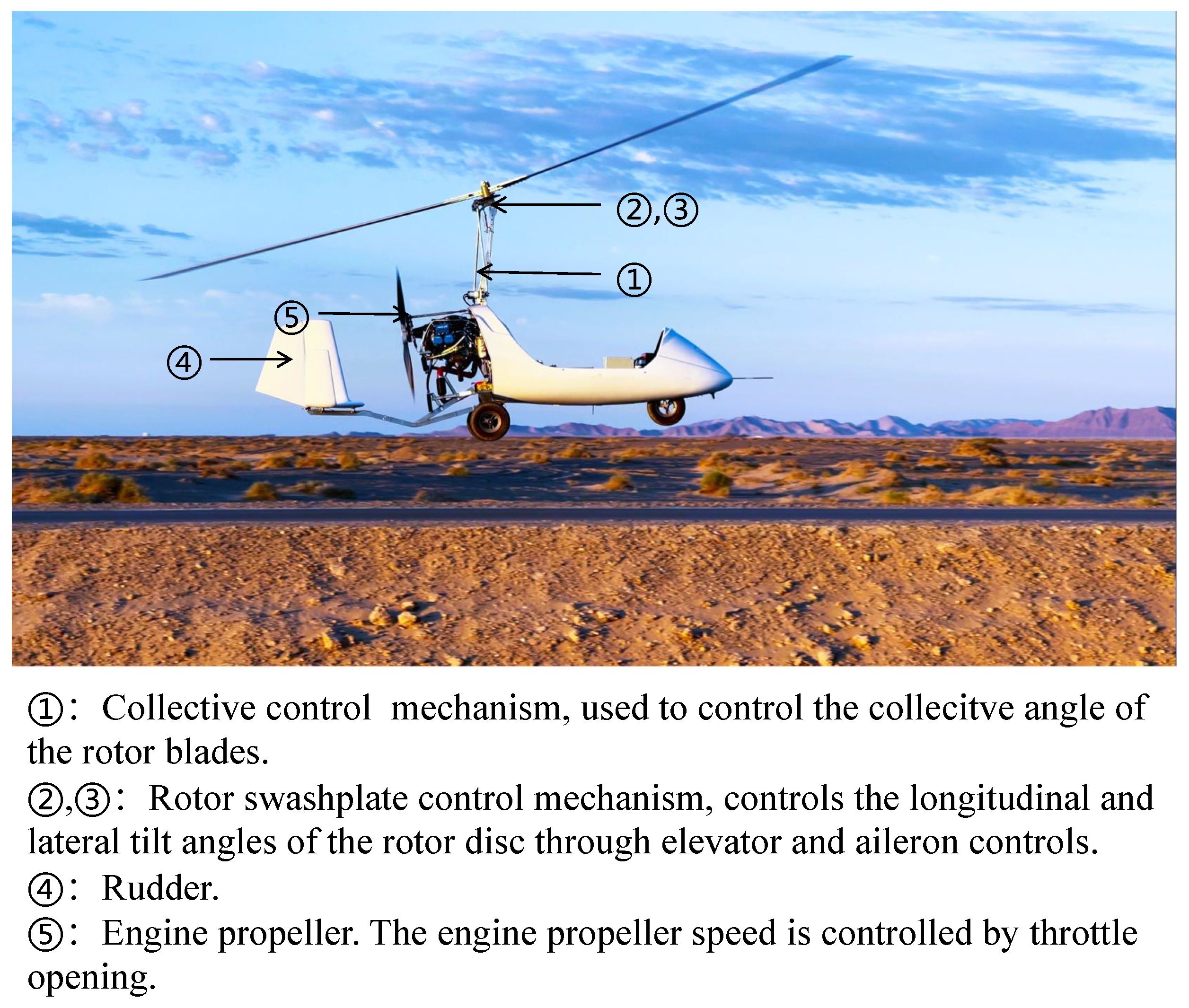
The appearance of an autogyro is very similar to that of a helicopter, with both having a large-diameter rotor on top that provides lift and aerodynamic torque for the aircraft. However, there are some noticeable differences. The rotor of a helicopter has a complex structure, is driven by an engine, and provides forward flight power, and achieving pitch and roll attitudes requires complex cyclic blade pitch changes. The rotor of an autogyro has a simple and reliable structure and is driven by airflow, while forward flight power is provided by the propeller, and achieving pitch and roll attitudes just requires tilting the rotor disc [5,6].

In the early twentieth century, many physicists studied the automatic rotation principle of rotors. The results that they obtained showed that under certain conditions, when a rotorcraft descends at an appropriate attack angle or flies horizontally, its rotor can rotate automatically. After that, there were a number of attempts to construct rotorcraft, but these did not have the capabilities of sustained and controlled flight. In the 1930s and 1940s, Juan de Cierva from Spain developed the first successful autogyro aircraft, the C-4 autogyro [7,8,9,10]. Because of its small size, simple structure, and low requirements for runway takeoff and landing, the success of the first autogyro has attracted widespread attention from society. Subsequently, many companies have invested in research on autogyros. Harold Pitcairn from America established the Pitcairn-Cierva Autogiro Company, which produced the PCA-2 autogyro with a flying speed of up to 190 km/h and a flying altitude of 5613 m. In 1953, the Bensen Aircraft Corporation produced the Bensen Gyrocopter, which had a simple structure, was easy to assemble, and required only a few dozen horsepower for takeoff and landing. Groen Brothers Aviation and Carter Aviation Technologies, two famous American rotorcraft companies, have been mainly dedicated to developing potential applications of rotorcraft [11]. In particular, the Carter Aviation Technologies’ CarterCopter, developed in 1998, combines the advantages of fixed-wing aircraft, tiltrotor aircraft, and helicopters. It can take off and land vertically, while also being capable of fast flight. At the beginning of the twenty-first century, AutoGyro from Germany became the world’s largest producer of autogyros, with its MTOsport autogyro having a long endurance time and being widely used, for example, in agriculture for plant protection and detection [12]. In addition, some research has been conducted on large jet-engine-based rotorcraft and unmanned rotorcraft, and this has yielded significant results [13,14,15,16,17].

China’s research on rotorcraft started later than that in Europe and America, with fewer achievements having been made so far. In recent years, however, Chinese enthusiasts have begun their own journey in developing rotorcraft and have played an important role in promoting research on autogyros.

Dynamic modeling is a prerequisite for flight control design and simulation, but owing to the complex aerodynamic characteristics of rotors, it is difficult to establish a high-confidence mathematical model for autogyros. Therefore, accurate rotor modeling is particularly important. The main methods for modeling rotor dynamics include momentum theory, blade element theory, vortex theory, wind tunnel experiments, and computational fluid dynamics (CFD) calculations, as well as some other methods [18].

At the end of the nineteenth century, Drzewiecki proposed the blade element theory for rotors, in which a rotor blade is considered as being composed of an infinite number of small blade elements [18,19]. The force and torque on a single blade or even the entire rotor can be obtained through radial integration. The advantage of this theory is its high accuracy, but it is complex to calculate and difficult to implement. In the early twentieth century, Glauert used momentum theory to model rotors in forward flight [20,21,22,23,24]. Momentum theory assumes uniform inflow and treats a rotor as an infinitely thin disc to study its effect on airflow using basic fluid dynamical laws. The advantage of momentum theory is its simplicity and efficiency in calculation, but because of the assumption of uniform induced velocity, it has reduced accuracy and a limited range of applicability. The results of wind tunnel experiments often differ significantly from actual flight data owing to the non-steady-state and nonlinear characteristics of rotor aircraft, as well as to the effects of wind tunnel size and interference from tunnel walls when using scaled models. CFD calculations are typically used for component analysis only, and so parameters calculated by CFD may differ significantly from their actual values for rotor aircraft with unsteady aerodynamic characteristics [18,20,21,22,23,24,25]. Currently, system identification is considered an effective method for establishing dynamic models for rotating wing aircraft. Glasgow University has developed a model based on system identification techniques [26]. However, modeling of rotorcraft dynamics based on system identification requires real helicopter flight data as a basis. If we want to study the effects on flight performance resulting from changes in the rotor parameters, this method has certain limitations.

Liu Peng and his team from Nanjing University of Aeronautics and Astronautics have conducted highly reliable modeling of helicopters based on FlightGear software [27]. The rotor part of an autogyro has almost identical dynamic characteristics to that of a helicopter, and the YASim dynamics library in FlightGear software has high confidence in modeling the rotor part. Therefore, the study described here is based on this library, taking account of the characteristics of autogyro rotors for secondary development, and adopting a simplification of traditional blade element theory to achieve greater accuracy in modeling autogyro rotor models.

Unlike a helicopter, which can directly drive its rotor to achieve the necessary rotation speed and lift for takeoff, an autogyro must use a different method. Typically, an autogyro uses its engine to drive the rotor for pre-rotation. After a certain rotation speed has been reached, the engine is disconnected from the rotor and used to drive the propeller for taxiing, which leads the autogyro to enter a spin state and increases the lift for takeoff. An autogyro has a simple rotor collective control system. As a result, the autogyro can obtain sufficient lift during the pre-selection stage by changing the collective angle and achieve vertical takeoff in a similar way to a helicopter. This takeoff method is called “jump-takeoff”, which is different from the takeoff methods of helicopters and fixed-wing aircraft and is based on the unique performance characteristics of autogyros [16].

Although the traditional takeoff method of an autogyro requires only a short distance of runway compared with fixed-wing aircraft, the autogyro still needs to taxi for tens to hundreds of meters before taking off, which imposes some requirements for the takeoff site and runway. However, with jump-takeoff, it is possible to achieve almost vertical takeoff in place like a helicopter, which greatly reduces the takeoff distance of an autogyro and further reduces its requirements in terms of takeoff site and runway. This increases the range of possible takeoff and landing sites for autogyros, opening up broader application prospects. Therefore, research on jump-takeoff for autogyros has great significance for engineering development and practical applications.

However, to date, there have been few studies of jump-takeoff of rotary-wing aircraft. In this article, accurate mathematical modeling based on YASim is conducted for a certain model of autogyro, design simulation solutions for the jump-takeoff of an autogyro are performed, the effects of different rotor parameters on jump-takeoff performance are examined, and guidance is provided for further optimization of jump-takeoff performance and for the design of rotor parameters. A complete jump-takeoff–climb–cruise mission is designed to verify the feasibility of jump-takeoff, lay the foundation for subsequent jump-takeoff experiments, and accumulate experience.

The remainder of this article is structured as follows. In Section 2, the mathematical model of the autogyro is briefly introduced. In Section 3, a simulation platform for the autogyro is constructed, on which verification validation and accreditation (VV&A) [28] are performed. In Section 4, the jump-takeoff conditions are explored and the jump-takeoff performance is studied. In Section 5, the jump-takeoff performance is optimized. In Section 6, a complete jump-takeoff–climb–cruise mission is implemented on the simulation platform based on optimized parameters. In Section 7, the main contributions of this study are summarized and conclusions are presented.

2. Mathematical Model for Autogyro

2.1. Rotor Dynamic Modeling Based on YASim

This article utilizes FlightGear’s YASim dynamic library to create a rotor modeling project that calculates the rotor force of the autogyro designed by Xiamen Univercity. By solving the dynamics of rotor flapping, we can determine the overall force on the rotor. To calculate this force, we use blade element theory to divide blade motion into eight directions and compute each microelement’s force at 0°, 45°, 90°, 135°, 180°, 225°, 270°, and 315°. The blades rotate counterclockwise. Traditional blade element theory requires the use of radial integration to obtain the forces and moments of the blades or even the entire rotor. The calculation is complex and simulation implementation is difficult. The simplified algorithm used here selects N micro-elements along the radial direction of the blade, calculates the aerodynamic force for each micro-element, simplifies integration into vector addition operations, and uses simulation algorithms to perform iterative calculations to obtain the required rotor forces and moments. This ensures calculation accuracy while avoiding difficulties in implementing integrals.

Starting from the basic equations of rotor blade flapping, assuming a stable rotation state of the rotor, and selecting a rigid blade with a center hinge as shown in Figure 1, we consider the external forces acting on the center of gravity of the rigid blade within the plane of flapping. These forces include the centrifugal force F, lift force T, and gravity G. In this case, we neglect inertial forces caused by blade flapping and assume that the moment exerted by the blade on its hinge is balanced.

The counterclockwise direction is taken as the positive direction for the torque and flapping angle $\beta$. Because during the rotation of the rotor, the flapping angle $\beta$ is actually a very small angle. Therefore, we make an approximation using small angles. Furthermore, the moment $M_G$ of the gravitational force G of the blade around the swing hinge is then given by:

$$M_G=-Mgrcos\beta \approx -Mgr,$$

(1)

where M is the blade mass. The centrifugal force F and the torque $M_F$ due to the blade’s rotational motion are as follows:

$$F=Mr{\Omega }^{2}cos\beta \approx Mr{\Omega }^2,$$

(2)

$$M_F=-Frsin\beta \approx Fr\beta ,$$

(3)

If the lift of the blade is T, then the moment of force around the flapping hinge due to lift is given by:

$$M_T=Tr,$$

(4)

The total moment of all these torques on the swinging hinge is zero, that is,

$$M_G+M_F+M_T=0,$$

(5)

The resulting equation for the flapping motion is

$$M_T=Fr\beta +Mgr,$$

(6)

which can be written as

$$M_T=\beta \left(Fr+\frac{Mgr}{\beta }\right),$$

(7)

Denoting $div=Fr+\frac{Mgr}{\beta }$, we obtain the following formula for calculating the angle of swing:

$$\beta =M_T/div,$$

(8)

By considering the effect of the airflow generated by the blade in the previous instant on the incident angle of the blade at the present instant and utilizing the initial value of the flap angle, denoted by ${\beta }_0$, a more accurate flap angle can be obtained through an iterative simulation algorithm. This enables us to calculate the force and torque of the rotor [27].

To calculate the lift of a rotor blade, it is divided into multiple small elements radially, and the lift of each element at different positions is calculated. The sum of the lifts of all these elements is then obtained to determine the overall lift and drag of the blade. This calculation takes into account the relationship between blade profile lift and drag with respect to angle of attack, which ultimately determines the lift and drag forces acting on the blade.

The lift and drag of the wing profile are, respectively:

$$L=\frac{1}{2}{C}_L\rho {\left|\overrightarrow{v}\right|}^2{A}_{\Delta r},$$

(9)

$$D=\frac{1}{2}{C}_D\rho {\left|\overrightarrow{v}\right|}^2{A}_{\Delta r},$$

(10)

where $\rho$ is air density, $C_L$ is the wing lift coefficient, $C_D$ is the wing drag coefficient, v is the sum of the velocities of the blade elements, and $A_{\Delta r}$ is the area of each element.

As shown in Figure 2, ${\alpha }_0$ represents the blade’s zero-lift angle of attack, ${\beta }_{*}$ represents the angle of attack, and w represents the direction of airflow.

Owing to the existence of an angle of attack ${\beta }_{*}$ between the lift L and the airfoil pull T of the airfoil, the airfoil pull T and rotational resistance of the airfoil Q are

$$T=Lcos{\beta }_{*}-Dsin{\beta }_{*},$$

(11)

$$Q=Dcos{\beta }_{*}+Lsin{\beta }_{*},$$

(12)

The lift moment of the blade and the wing twist torque are then

$$M_T=T·r=\left(Lcos{\beta }_{*}-Dsin{\beta }_{*}\right)·r,$$

(13)

$$M_Q=Q·r=\left(Dcos{\beta }_{*}+Lsin{\beta }_{*}\right)·r,$$

(14)

When an autogyro performs pitch or roll movements, the rotor shaft moves together with the fuselage, having the same angular velocity. Due to the fact that the blades and rotor shaft are not fixed together and do not tilt synchronously, an angle difference occurs, known as flapping, for the autogyro. When the angular movement of the autogyro stops, the rotor will follow along under the influence of aerodynamic forces. We take the angular velocity of the autogyro as $\overrightarrow{rot}=\left[\begin{array}{c}{\omega }_x\\ {\omega }_y\\ {\omega }_z\end{array}\right]$. The projection of its angular velocity in the direction of the rotor’s normal vector can be used to represent the motion trend of the autogyro.

$$a=\overrightarrow{rot}\odot \overrightarrow{normal}$$

(15)

If a > 0, it indicates that the autogyro is in an upward trend. At this time, the initial value of the flapping angle ${\beta }_0$ is determined by iterative calculation to obtain the flapping angle $\beta$, as well as the flapping angle at the position where the rotor continues to rotate 90° after this moment.

$${\beta }_0=\beta cosa+{\beta }_{next90}sina$$

(16)

If a < 0, it indicates that the helicopter is in a descending trend. At this time, the initial value of the flapping angle ${\beta }_0$ is determined by iterative calculation to obtain the flapping angle $\beta$, together with the flapping angle at the position where the rotor has rotated 90° before this moment.

$${\beta }_0=\beta cosa-{\beta }_{last90}sina$$

(17)

According to the previous sections, we can obtain the flapping angle of the rotor at different times and positions through an iterative method. Considering the mutual influence of blade flapping at different positions, an average flapping angle is adopted for the blades based on the flapping angles in four directions, and a swing factor $S_{factor}$ is introduced:

$${\left(cos\beta \right)}_{mean}={\left(cos\beta \right\}}_{next90}+cos{\beta }_{last90}+cos\beta +{cos\beta }_{oppsite})/4,$$

(18)

$$S_{factor}=1-\left(cos\beta -{\left(cos\beta \right)}_{mean}\right)·N/4,$$

(19)

where N is the number of blade elements. Therefore, the vertical and horizontal forces generated by the rotor are, respectively,

$$F_Z=S_{factor}·F·sin\beta {·F}_{lift},$$

(20)

$$F_X=F·tcos\beta ,$$

(21)

where $F_{lift}$ is the lift factor, which is usually a constant, and F is centrifugal force.

2.2. Rotor Dynamic Modeling Based on YASim

In order to calculate the stable rotation speed of the rotor, it is necessary to solve a nonlinear equation [29,30]. The rotor modeling platform uses an iterative method to calculate and determine stable spinning. Based on the input power $P_E$ of the engine to the rotor, the output power $P_R$ of the rotor’s torque on air at current speed, and the output power $P_J$ of the rotor, we can calculate a rotation speed increase/decrease coefficient $\zeta$, which is a dimensionless coefficient.

$$\frac{d\zeta }{dt}=\frac{P_E-P_R}{P_J},$$

(22)

$$\zeta =\int \frac{P_E-P_R}{P_J}dt,$$

(23)

During the rotation of the rotor, the engine and rotor connection mechanism disconnects. Therefore, the engine does almost no work on the rotor. The only input power for the rotor comes from friction between the connection mechanism of the engine and rotor, which is a constant power represented as $P_f$.

$$P_E=-P_f,$$

(24)

$P_f$ is generally very small and can be ignored, therefore:

$$P_E=-P_f=0,$$

(25)

The formula for calculating the output power of a rotor to the air is:

$$P_R=-M_Q·{\Omega }_0,$$

(26)

The formula for calculating the output power of a rotor is:

$$P_J=\frac{d{E}_J}{dt}=\frac{dJ·{\omega }_0^2}{dt}=\frac{d\frac{J·{\Omega }_0^2}{4{\pi }^2}}{dt}=\frac{J·{\Omega }_0·{\alpha }_0}{2\pi },$$

(27)

where J is the moment of inertia of the rotor, ${\Omega }_0$ is the initial rotation speed of the rotor, and ${\alpha }_0$ is the initial angular acceleration of the rotor.

The formula for calculating the speed increase/decrease coefficient, based on Equations (22) to (27), can now be written as

$$\zeta =\int \frac{-P_f+M_Q·{\Omega }_0}{\frac{J·{\Omega }_0·{\alpha }_0}{2\pi }}dt=2\pi \int \frac{M_Q}{J·{\alpha }_0}dt,$$

(28)

Furthermore, we can obtain the following expression for the rotation speed at each instant.

$$\Omega ={\Omega }_0·\zeta ,$$

(29)

By combining Equations (28) and (29), it can be observed that when the rotor blade torque is negative ($M_Q$ < 0), the aerodynamic force does negative work on the rotor blade, the rate of change of the rotation speed increase/decrease coefficient $\frac{d\zeta }{dt}$ < 0, the rotation speed increase/decrease coefficient $\zeta$ decreases, the rotation speed $\Omega$ gradually decreases, and the lift gradually decreases. When the rotor blade torque is positive ($M_Q$ > 0), the aerodynamic force does positive work on it, the rate of change of the rotation speed increase/decrease coefficient $\frac{d\zeta }{dt}$ > 0, the rotation speed increase/decrease coefficient $\zeta$ increases, the rotation speed $\Omega$ gradually increases, and the rotor enters an auto-rotation state with increasing lift. When the rotor blade torque is zero ($M_Q$ = 0), no work is performed by aerodynamic forces on the rotor blade, the rate of change of rotation speed increase/decrease coefficient $\frac{d\zeta }{dt}=0$, the rotation speed increase/decrease coefficient $\zeta$ remains stable, and the rotation speed $\Omega$ stabilizes gradually along with lift to achieve steady auto-rotation. All results are shown in the

Table 1. All results of change of rotation speed.

${\mathit{M}}_{\mathit{Q}}$	$\frac{\mathit{d}\mathit{\zeta }}{\mathit{dt}}$	$\mathit{\zeta }$	$\Omega$	Lift
>0	<0	increase	increase	increase
<0	>0	decrease	decrease	decrease
=0	=0	-	-	-

.

Therefore, we can obtain the criteria for rotor stability spin, namely, the rotor generates an upward vertical lift equal to gravity, while the torque of the rotor’s airfoil is zero [30]:

$$F_Z=mg,$$

(30)

$$M_Q=0,$$

(31)

3. Establishment of Simulation Platform

3.1. Autogyro Overview

The research in this paper focuses on a particular autogyro model, which adopts a conventional autogyro configuration, consisting of a teetering rotor with fixed pitch, a piston-engine-driven propeller, a rudder, a fuselage, and a tricycle landing gear [31,32]. It has four control surfaces, consisting of longitudinal and lateral tilting of the rotor disc, engine throttle opening, and rudder. This autogyro model has a takeoff weight of 450 kg, making it a small unmanned aircraft. The main overall parameters are shown in

Table 2. Main overall parameters of the research object.

Parameters	Value
Takeoff Weight (kg)	450
Rotor Diameter (m)	8.5
Chord (m)	0.218
Twist (°)	0
Taper (°)	1
Collective (°)	0–13
Number of rotor Blades (-)	2
Number of Propeller Blades (-)	3
Blade Weights (pounds)	36

.

We selected the parameters of the autogyro from Table 2, based on the lift coefficient and drag coefficient of the blade NACA 8-H-12 at different attack angles in

Table 3. Main rotor lift coefficient and drag coefficient table.

Alpha	CL	CD
−5	−0.3908	0.0184
−4.5	−0.34	0.0157
−4	−2.874	0.0144
−3.5	−0.2343	0.0135
−3	−0.182	0.0125
−2.5	−0.1304	0.0115
−2	−0.076	0.0111
−1.5	−0.0224	0.0105
−1	0.0281	0.0097
−0.5	0.0609	0.0076
0.5	0.3016	0.0081
1.5	0.4320	0.0081
2	0.4830	0.0082
2.5	0.5342	0.0084
3	0.5863	0.0085
3.5	0.6383	0.0086
4	0.6899	0.0089
4.5	0.7422	0.0091
5	0.7943	0.0093
5.5	0.8461	0.0095
6	0.8978	0.0096
6.5	0.9500	0.0096
7	1.0019	0.0098
7.5	1.0531	0.0101
8	1.1007	0.0109
8.5	1.1280	0.0142
9	1.1445	0.0173
9.5	1.1392	0.0202
10	1.1307	0.0231
10.5	1.1189	0.0272
11	1.1186	0.0310
11.5	1.1164	0.0352
12	1.1146	0.0398
12.5	1.1122	0.0449
13	1.1047	0.0507

, modeled it based on the modeling mechanism for autogyro dynamics described in Section 2, and connected it to the flight control system to establish a simulation platform for the autogyro as shown in Figure 3. The control variables displayed in this simulation platform correspond to the control mechanisms in a real autogyro as shown in the Figure 4. With this simulation platform, we will verify our autogyro model, design jump-takeoff experiments, and study autogyro jump-takeoff performance.

3.2. Stable Rotation Analysis

In Section 2.2, we studied the basic principles of rotor steady auto-rotation. It is important to determine whether a rotor can achieve steady auto-rotation. Therefore, in this subsection, we will use the autogyro simulation platform established in Section 3.1 to explore the steady auto-rotation speed for different collective angles, as shown in

Table 4. Steady-state rotation speed of autogyro models under various collectives.

Collective (${}^{°}$)	1	2	3	4	5	6	7	8	9	10	11	12	13
$\Omega$ (RPM)	450.9	373.7	322.6	288.9	264.6	242.9	224.4	210.9	205	196.9	191	187	182.3

and Figure 5. The results not only verify the accuracy of the model, but also provide guidance for the design of collective control during the transition phase after jump-takeoff.

From Table 4 and Figure 5, it can be seen that at the same airspeed of autogyro, the stable spin speed of a autogyro decreases with an increase in the collective angle. Moreover, when the collective angle is less than 8${}^{°}$, increasing the collective angle has a significant effect on reducing the stable spin speed. A lower stable spin speed can reduce the blade tip linear velocity and decrease rotor drag, which has some significance for further improving the airspeed of the autogyro.

3.3. Reliability Analysis

Models must be built on a foundation of the correct concepts. Their credibility can be measured through planned verification and validation work, which constitutes the process of models verification and validation [28,33].

Model verification consists of proving that the model can be transformed from one form to another, as intended, with sufficient accuracy. It is concerned with showing that the model has been constructed in the right way. The accuracy with which a problem formulation can be transformed into a model specification or with which a model representation can be converted from a micro-flowchart form into an executable computer program is evaluated in model verification [28]. Model validation consists of proving that the model, within its domain of applicability, behaves with satisfactory accuracy consistent with the modeling and simulation (M&S) objectives. It is concerned with showing that the right model has been constructed [28]. We will validate our model specifically through the use of static and dynamic techniques.

Static techniques can verify a large amount of information, such as model structure, modeling techniques, data in the model, control flow, and syntax accuracy [33]. In this article, we mainly verify the data and control flow in the model through the use of static techniques. We have programmed our model with the same physical parameters and control commands as in a real aircraft to ensure that it accurately reflects the behavior of the actual model during simulation. The specific parameter settings are shown in

Table 5. Physical parameters and control commands.

Parameters	Actual Flight Data	Simulation Data
Takeoff Weight (kg)	450	450
Rotor Diameter (m)	8.5	8.5
Height Command (m)	1910	1910
Velocity Command (m/s)	30.5	30.5
Elevator Command (°)	8.7	8.7
Aileron Command (°)	1.2	1.2
Collective Command (°)	2	2

.

Dynamic techniques require the running of models and analysis of the correctness of the model based on the behavior during the running process and the final results [33]. By running a simulation platform for the autogyro model, we can obtain the process and results of simulating the model based on the control instructions that were initially set. To verify the reliability of the entire simulation process, we set up three key links for testing during the process of solving the rotor model: the detection of the direction of the centripetal force in blade element theory, the detection of rotor lift, and the detection of the rotor blade torque and the rate of change of the rotation speed coefficient. These three tests will, respectively, verify the correctness of the blade element theory solution process, the correctness of the rotor aerodynamic force calculation, and the correctness of the rotor auto-rotation process. The results are described below. In addition, we compare our final simulation results with actual flight data from this autogyro to analyze them and to validate the accuracy of the model. The results are also presented in

Table 6. Vector coordinates of the centripetal force direction when the blade rotates.

Blade Rotation Angle	Vector Coordinates
	X	Y	Z
0${}^{°}$	0.00	1.00	0.00
45${}^{°}$	−0.71	0.71	0.00
90${}^{°}$	−1.00	0.00	0.00
135${}^{°}$	−0.71	−0.71	0.00
180${}^{°}$	0.00	−1.00	0.00
225${}^{°}$	0.71	−0.71	0.00
270${}^{°}$	1.00	0.00	0.00
315${}^{°}$	0.71	0.71	0.00

and Figure 6 and Figure 7.

Table 6 shows that during the simulation calculation, when the blade element rotates to each position, the calculated centripetal force is correctly allocated in the correct direction. This verifies the correctness of the blade element theory calculation. Figure 6 shows the vertical force generated by the rotor in level flight simulation. Owing to the shape of the aircraft body, a certain amount of downward pressure is produced, and so the calculated vertical force needs to be slightly greater than gravity, which verifies the correctness of the rotor force and torque calculation. Figure 7 shows the changes in rotor torque and the speed increase/decrease coefficient rate during level flight simulation. It can be seen that in the simulation, after stable flight has been entered, both the wing twist torque and the speed increase/decrease coefficient rate are 0. These results show that the model simulation has entered a stable spin state, and thus verify the correctness of the spin model.

The simulation results are compared with actual flying data under similar conditions in Figure 8, Figure 9, Figure 10, Figure 11, Figure 12, Figure 13, Figure 14 and Figure 15. It can be seen that the simulation results for altitude and velocity are consistent with the actual flight data. Those for the throttle and rotor stable speed are also similar to the actual flight data, with an error within 5%. However, there is some deviation between the simulation results and the actual flight data for pitch angle, elevator, roll angle, and aileron. Nevertheless, based on engineering experience, these deviations fall within a reasonable range. These results indicate a high level of reliability in the simulation model and provide a solid foundation for subsequent jump-flight simulations.

The verification using the above mentioned static and dynamic techniques has ensured that the modeling and simulation both have a high degree of confidence. In the following sections, we will use this simulation platform to design experiments on jump-takeoff of the autogyro.

3.4. Design of the Jump Takeoff Experiment

The engine is started and the rotor is driven by the transmission mechanism at a rotation speed exceeding that required for normal flight, generally up to 150–200% of the normal rotation speed. Then, the engine disengages from the rotor, and the collective angle is quickly changed to the angle required for takeoff. The resulting lift makes the autogyro ascend vertically into the air and achieve vertical takeoff [34,35,36,37,38]. When the rotation speed decreases, total distance to reach the self-rotation angle is decreased, and the tail push propeller is used to provide forward thrust force so that the autogyro can fly forward in a stable manner. Two indicators define good or bad jump-takeoff performance, namely, jump height and rotation speed decay rate. A higher jump height is achieved with a slower rotation speed decay rate, indicating better jump-takeoff performance.

We used the parameters of the autogyro rotor to construct a pseudo-six-degrees-of-freedom model (mass block). Except for the rotor part, the fuselage was treated as a mass block. The default setting assumed that the three-axis force and torque were in equilibrium (except for longitudinal jump-takeoff force). We neglected the impact of air resistance and the airflow during jump-takeoff on the autogyro’s fuselage. The wind speed was set to zero. We set an initial rotation speed so that the autogyro could achieve vertical takeoff with significant lift. Since this was an unpowered jump-takeoff, the autogyro only has vertical movement and no forward or sideways motion. The rotor of an autogyro does not rely on airflow to rotate, so the rotation speed gradually decreases due to friction at the hub and air resistance. As a result, the lift generated by the rotor decreases, causing the autogyro to descend after reaching its highest point and eventually land back on the ground.

4. Implementation of Jump-Takeoff

4.1. Jump-Takeoff Conditions

The basic condition for successful jump-takeoff is

$$L_{0max}>mg,$$

(32)

where $L_{0max}$ is the maximum lift generated by the pre-rotation stage rotor and m is the total takeoff mass of the autogyro. To achieve jump-takeoff in a particular autogyro, coordination between various pre-rotation speeds, which is represented as $\omega$, and the collective angle is necessary. We have therefore defined a minimum pre-rotation condition and a minimum collective angle condition for jump-takeoff.

• The minimum pre-rotation condition: the minimum pre-rotation speed that satisfies the condition for successful jump-takeoff. The maximum collective angle of the autogyro studied in this article is 13${}^{°}$, and so the minimum pre-rotation condition for jump-takeoff is when the collective angle is 13${}^{°}$ and the pre-rotation speed satisfies the condition for successful jump-takeoff. We use ${\omega }_{min}$ to represent the minimum pre-rotation speed.
• The minimum collective angle condition: The minimum collective angle that satisfies the condition for successful jump-takeoff. In theory, as long as the collective angle is greater than 0${}^{°}$, the condition for successful jump-takeoff can be met at a sufficiently high pre-rotation speed. However, the pre-rotation speed cannot always be high, owing to material performance limitations and the transmission efficiency of engine and rotor connection devices. The maximum theoretical pre-rotation speed is about 150–200% of the maximum normal flight speed. The cruising rotation speed of the self-rotating rotor aircraft studied in this article is about 380 rpm, and so the maximum theoretical pre-rotation speed is about 560 rpm. The minimum collective angle condition is the collective angle that satisfies the condition for successful jump-takeoff when the pre-rotation speed is 560 rpm.

Based on the minimum pre-rotation condition and the minimum collective angle condition, we explored the minimum jump-takeoff conditions for intermediate states. The results are shown in

Table 7. The minimum jump takeoff conditions under various collectives.

Collective (°)	${\mathit{\omega }}_{\mathit{min}}$ (RPM)	mg (N)	L (N)	L > mg
13	288	4410	4423	✔
12	297	4410	4434	✔
11	307	4410	4436	✔
10	318	4410	4420	✔
9	332	4410	4445	✔
8	347	4410	4417	✔
7	366	4410	4413	✔
6	390	4410	4417	✔
5	421	4410	4421	✔
4	463	4410	4418	✔
3	525	4410	4413	✔
2.6	560	4410	4419	✔

.

The minimum jump-takeoff condition curve can be obtained from Table 7. This curve, together with the maximum collective angle limit and the maximum pre-rotation speed limit conditions, encloses a closed area called the jump-takeoff condition envelope, as shown in Figure 16. Any combination of collective angle and pre-rotation speed at any point within the takeoff condition envelope can achieve jump-takeoff for an autogyro.

4.2. Simulation Results

The jump-takeoff heights of the autogyro in the jump-takeoff envelope are shown in

Table 8. Jump-takeoff heights (m) in different states in the jump-takeoff envelope.

Collective (°)	$\mathit{\omega }$ (RPM)
	560	520	480	440	400	360	320	288
13	55.08	37.64	23.75	13.30	6.13	1.94	0.22	0.00
12	58.40	39.27	24.21	13.07	5.65	1.56	0.11	0.00
11	61.40	40.47	24.22	12.49	4.96	1.12	0.03	0.00
10	63.65	40.91	23.58	11.42	4.03	0.67	0.00	0.00
9	64.52	40.11	21.97	9.76	2.88	0.27	0.00	0.00
8	63.01	37.42	19.07	7.44	1.62	0.03	0.00	0.00
7	57.78	32.08	14.62	4.58	0.53	0.00	0.00	0.00
6	47.31	23.56	8.84	1.76	0.02	0.00	0.00	0.00
5	31.02	12.55	3.05	0.13	0.00	0.00	0.00	0.00
4	12.08	2.78	0.09	0.00	0.00	0.00	0.00	0.00
3	0.60	0.00	0.00	0.00	0.00	0.00	0.00	0.00
2.6	0.00	0.00	0.00	0.00	0.00	0.00	0.00	0.00

. The height variation curve of the jump height in the jump-takeoff envelope drawn from the data in the table is shown in Figure 17. It can be seen from this figure that when the minimum jump-takeoff requirement is satisfied, for any collective angle, the higher the pre-rotation speed of the autogyro, the higher is its jump-takeoff height. However, there is a limit to the pre-rotation speed owing to the disconnection between engine and main rotor transmission after completion of pre-selection by the auto-rotation blades. Increasing the collective angle does not always lead to an increase in jump-takeoff height at any given pre-rotation speed. When the pre-rotation speed is less than 440 rpm, the maximum jump-takeoff height is achieved at a collective angle of 13°, but when it exceeds 440 rpm, the maximum jump-takeoff height is reached at a collective angle of about 10° and decreases as the collective angle continues to exceed that value. This is because too high a collective angle generates significant resistance, which reduces the lift generated by the rotor. Furthermore, the negative effects of a high collective angle on jump-takeoff height become more pronounced as the pre-rotation speed increases.

Owing to limitations of the rotor drive mechanism, a jump-takeoff pre-rotation speed of 400 rpm was selected. Under this certain pre-rotation speed, we continue to perform the jump-takeoff simulation and obtain the graph of height change of jump-takeoff as shown in the Figure 18. The change in rotation speed decay rate during jump-takeoff with different collective angles at this pre-rotation speed was explored. The speed attenuation data obtained from the experiment were fitted by polynomial regression to obtain the speed attenuation curve at different collective angles. The derivative of the speed attenuation curve was calculated to obtain the speed attenuation rate curve at different collective angles, as shown in Figure 19a,b. We can see that the speed attenuation rates at different collective angles all exhibit a logarithmic trend, gradually decreasing and converging to nearly the same value over time, and so the average of the angular velocity attenuation rate can be used as a evaluation index to represent the process as a whole.

The average and initial rotation speed decay rates during the entire jump-takeoff process at different collective angles are shown in

Table 9. Average and initial rotation speed decay rates at different collective angles and 400 rpm.

Collective (°)	13	12	11	10	9	8	7	6
Average rate (rev/min/s)	75.57	71.21	66.96	63.01	59.32	55.97	53.19	51.8
Initial rate (rev/min/s)	197	171.1	146.9	124.6	104.3	85.95	69.74	55.69

. It can be seen that as the collective angle decreases, both the average and initial rotation speed decay rates exhibit a monotonic decrease. This indicates that at a smaller collective angle, the rotation speed decay rate of the entire process is smaller, and thus better jump-takeoff performance can be achieved. Since the differences in the initial rotation speed decay rate at different collective angles are more significant and this rate is easier to calculate, we adopt it to represent the overall rotation speed decay rate for further study. The variations in average and initial rotation speed decay rates obtained from the data in Table 9 are plotted in Figure 20.

5. Performance Optimization for Jump Takeoff

Based on the analysis of the jump-takeoff performance in Section 4, and considering the performance of the transmission mechanism between the engine and rotor as well as the maximum collective angle jump-takeoff limit, a pre-rotation speed of 400 rpm and a collective angle of 10° were determined for jump-takeoff. According to the conclusion in Section 4 and the analysis in Section 3.4, we will optimize the jump-takeoff performance. There are two main aspects of optimization. On one hand, we need to generate more lift during the jump-takeoff process to increase the jump-takeoff height of the autogyro. On the other hand, we need to reduce the rotation speed decay rate. To achieve these two points, we will explore and optimize the jump-takeoff performance by changing two rotor parameters: rotor diameter and blade tip weighting. The method of adding weights to the tip of rotor blades is called blade tip weighting. As we known, tip weight weighting can increase the rotational inertia of the rotor.

A high-inertia rotor can store a large amount of energy that can be transformed into the initial take-off force, and it can store more energy to bring about greater jump-takeoff performance. Furthermore, it can also provide greater centrifugal force, which prevents instability caused by blade bending during rotation [36,38,39].

For convenience in the modeling and simulation calculations in this article, the added weight block at the blade tip is considered as mass point, and its rotational inertia is thus obtained as

$$J_{tip}=\frac{1}{2}{M}_{tip}R,$$

(33)

where $M_{tip}$ is the added mass at the blade tip and R is the radius of the rotor. When there is no additional weight attached to the end of the rotor blade, the rotational inertia of the blade is

$$J_{rotor}=\frac{1}{12}M{l}^2,$$

(34)

where M is the mass of a single blade and l is the diameter of the rotor plane. Therefore, the rotational inertia of the rotor blade with additional weight added to its tip is

$$J_{rotor}=J_{tip}+J_{rotor}=\frac{1}{12}M{l}^2+\frac{1}{2}{M}_{tip}R,$$

(35)

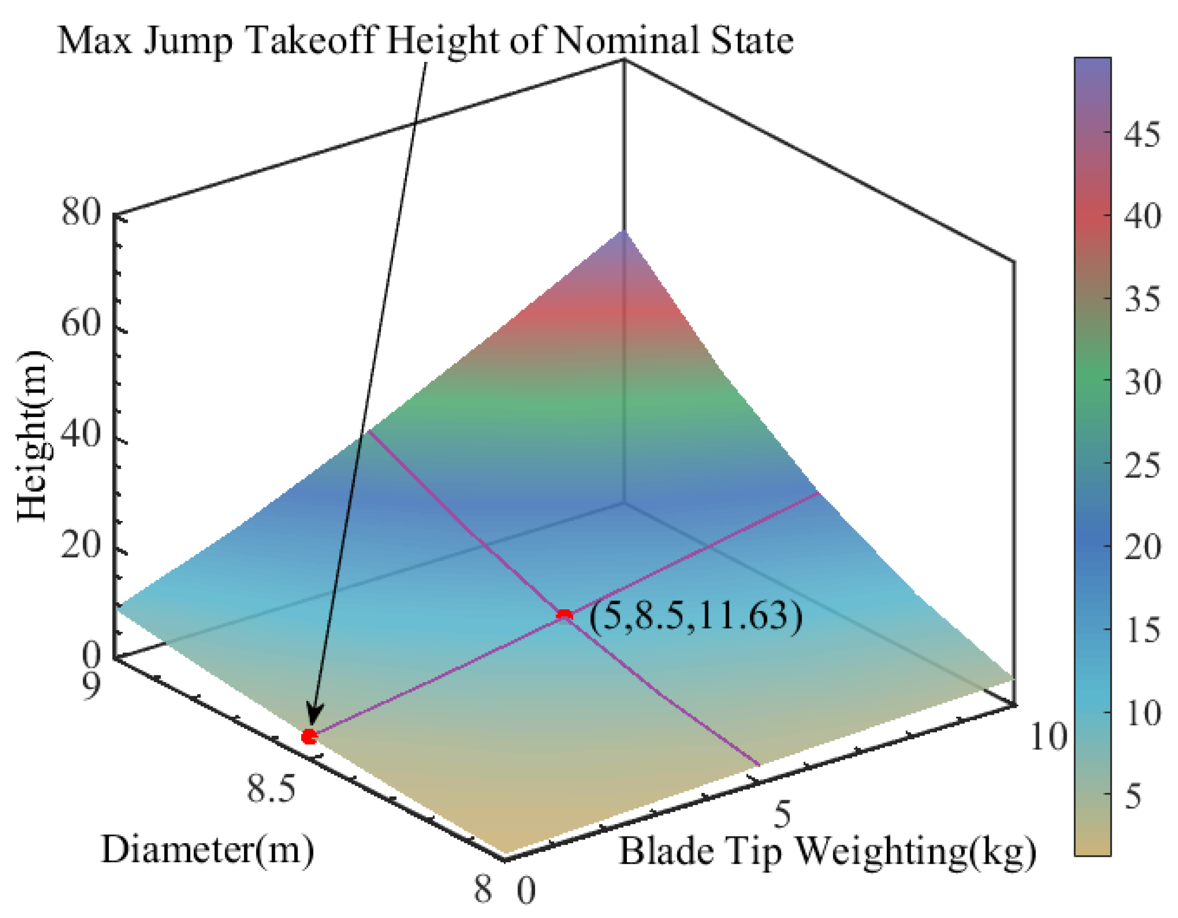
Based on the weight of the rotor blade itself, the maximum blade tip weighting setting should not exceed 65% of the weight of the rotor blade. The range of variation of the rotor diameter should be within 6% of the diameter. Therefore, the diameter was varied from 8 m to 9 m in increments of 0.25 m, and the blade tip weighting was varied from 0 kg to 10 kg in increments of 2.5 kg. Jump-takeoff flight experiments were conducted for different combinations of rotor parameters, and the results are shown in

Table 10. Jump-takeoff height (m) for different values of rotor diameter and blade tip weighting.

Diameter (m)	Blade Tip Weightings (kg)
	0	2.5	5	7.5	10
8	1.21	2.14	3.09	3.95	4.67
8.25	2.38	4.37	6.55	8.73	10.78
8.5	4.03	7.57	11.63	15.89	20.12
8.75	6.19	11.82	18.44	25.61	32.99
9	8.87	17.14	27.05	38.02	49.56

. The variations in jump-takeoff height obtained from the data in Table 10 are plotted in three dimensions in Figure 21.

As can be seen from Figure 21 and Table 10, overall, the jump-takeoff height increases with increasing blade tip weighting and rotor diameter. However, when the blade tip weighting is small, the sensitivity of the jump-takeoff height to changes in rotor diameter is low. Similarly, when the rotor diameter is small, the sensitivity of the jump-takeoff height to changes in tip weight is low. Further analysis reveals that within the area enclosed by two curves representing a fixed rotor diameter of 8.5 m with varying tip weight and a fixed blade tip weighting of 5 kg with varying rotor diameter, the maximum jump-takeoff height is generally optimized within a range of 10 m or less. Beyond this range, there is a high sensitivity of the maximum jump-takeoff height to both rotor diameter and blade tip weighting, and even slight increases in either parameter can significantly change the maximum jump-takeoff height.

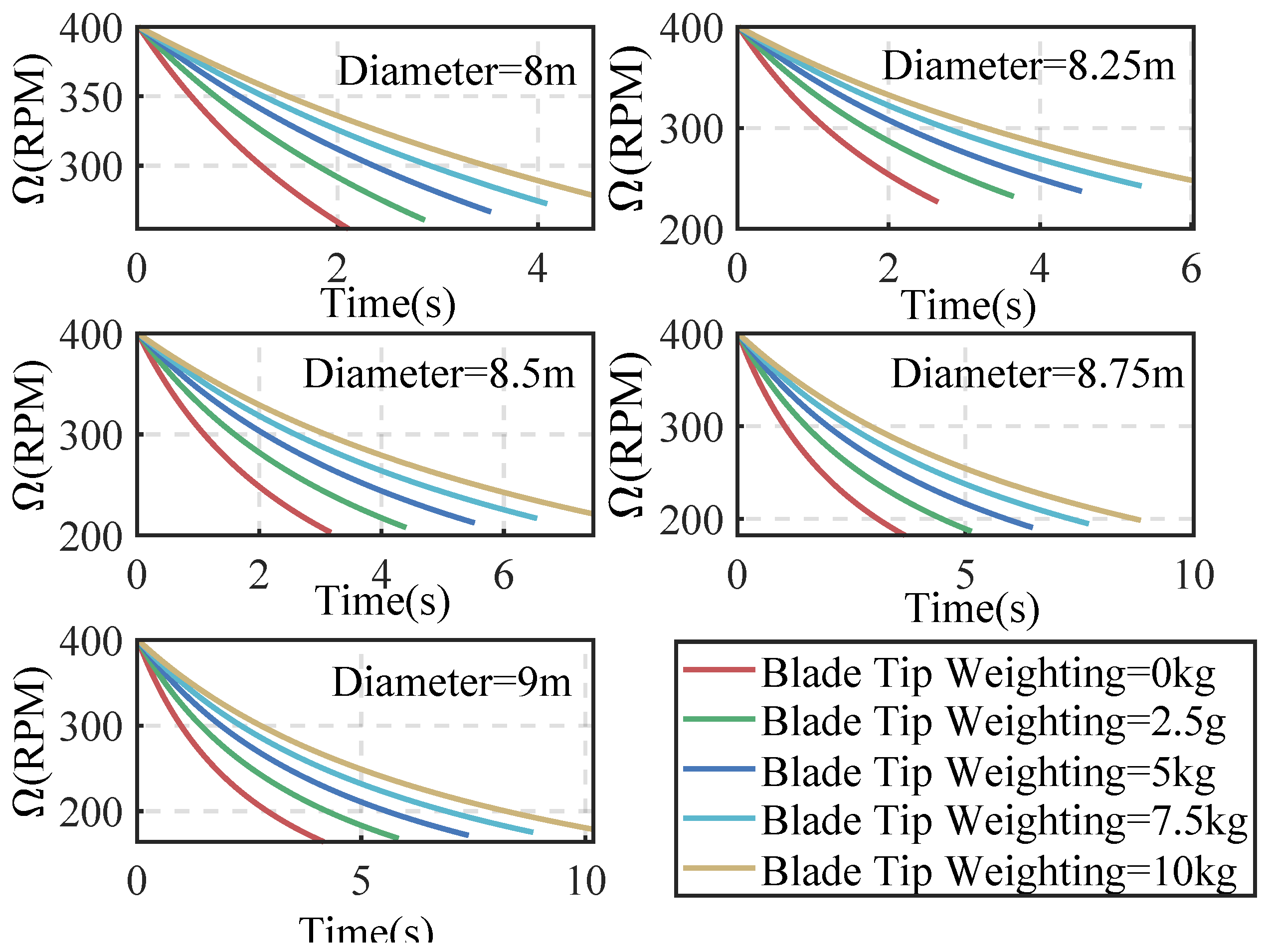
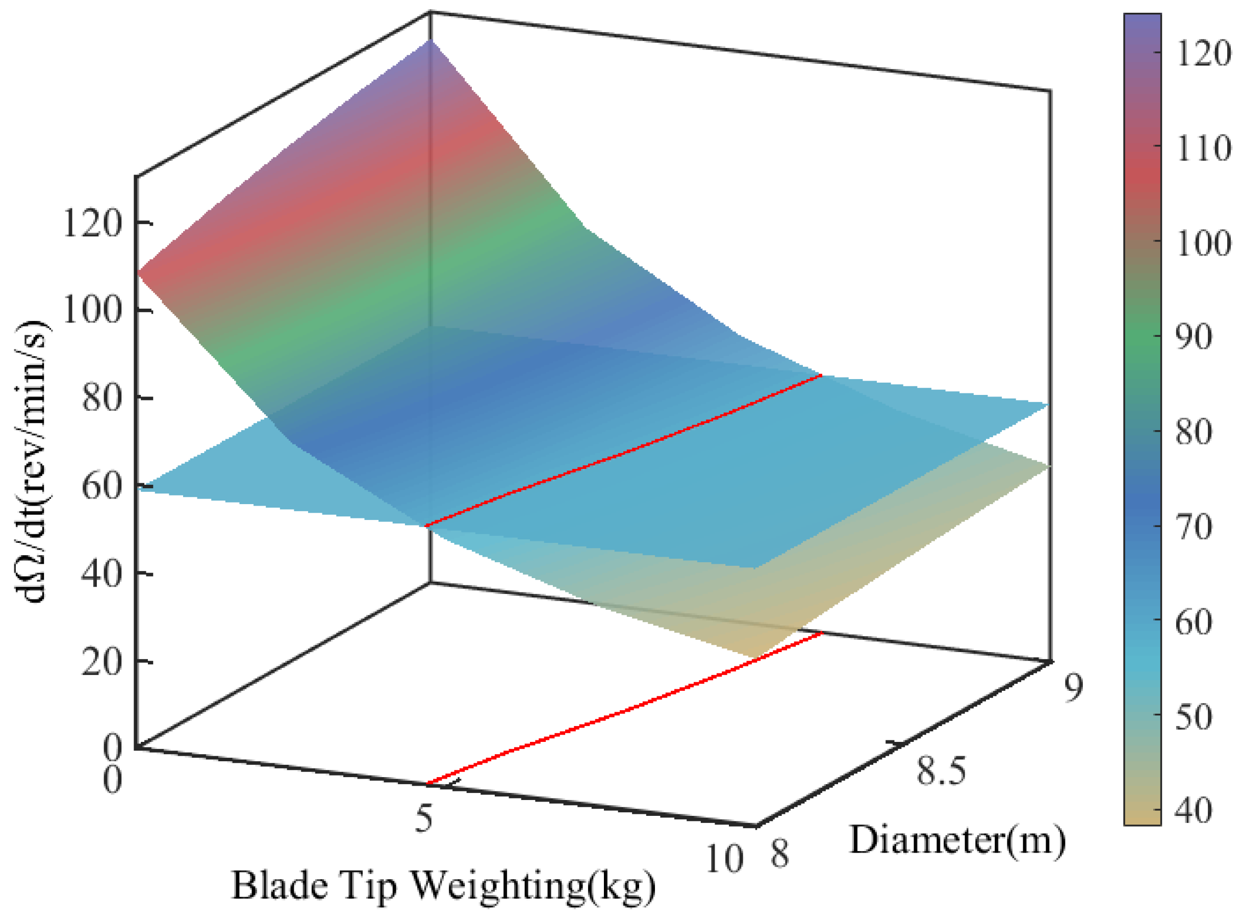
From Figure 22, it can be seen that there are significant differences in the rotation speed decay for different blade tip weighting and rotor diameters. The smaller the rotor diameter and the heavier the blade tip weighting, the slower the rotation speed decays. On the basis of the results obtained in Section 4.2, we chose the initial state speed decay rate at different parameter values to represent the overall speed decay rate of the process. By fitting a polynomial function to the curve of rotation speed decay, we can differentiate at the initial state point to obtain an initial rate of decay for each combination of rotor parameters, as shown in

Table 11. Rotation speed decay rate (rev/min/s) of initial state for different values of rotor diameter and blade tip weighting.

Diameter (m)	Blade Tip Weighting (kg)
	0	2.5	5	7.5	10
8	108.3	74.13	56.4	45.54	38.21
8.25	113.2	77.59	59.09	47.77	40.12
8.5	117.5	80.63	61.49	49.75	41.83
8.75	121.2	83.22	63.53	51.47	43.31
9	124.1	85.38	65.24	52.91	44.56

. The variations in rotation speed decay rate obtained from the data in Table 11 are plotted in three dimensions in Figure 23.

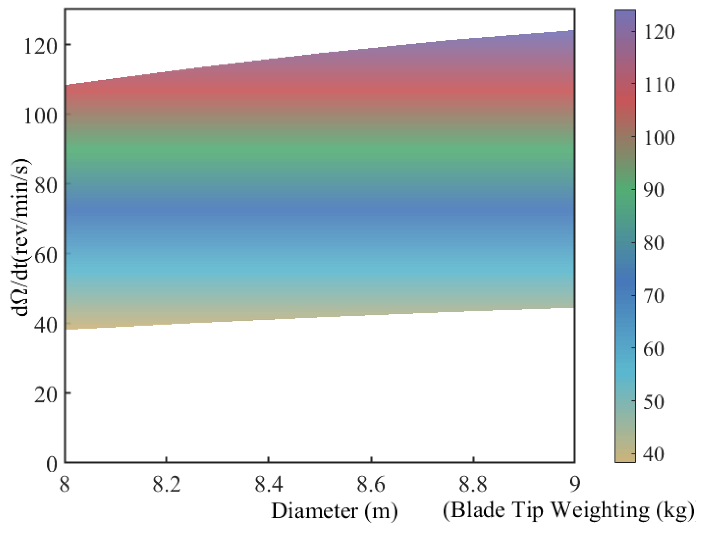
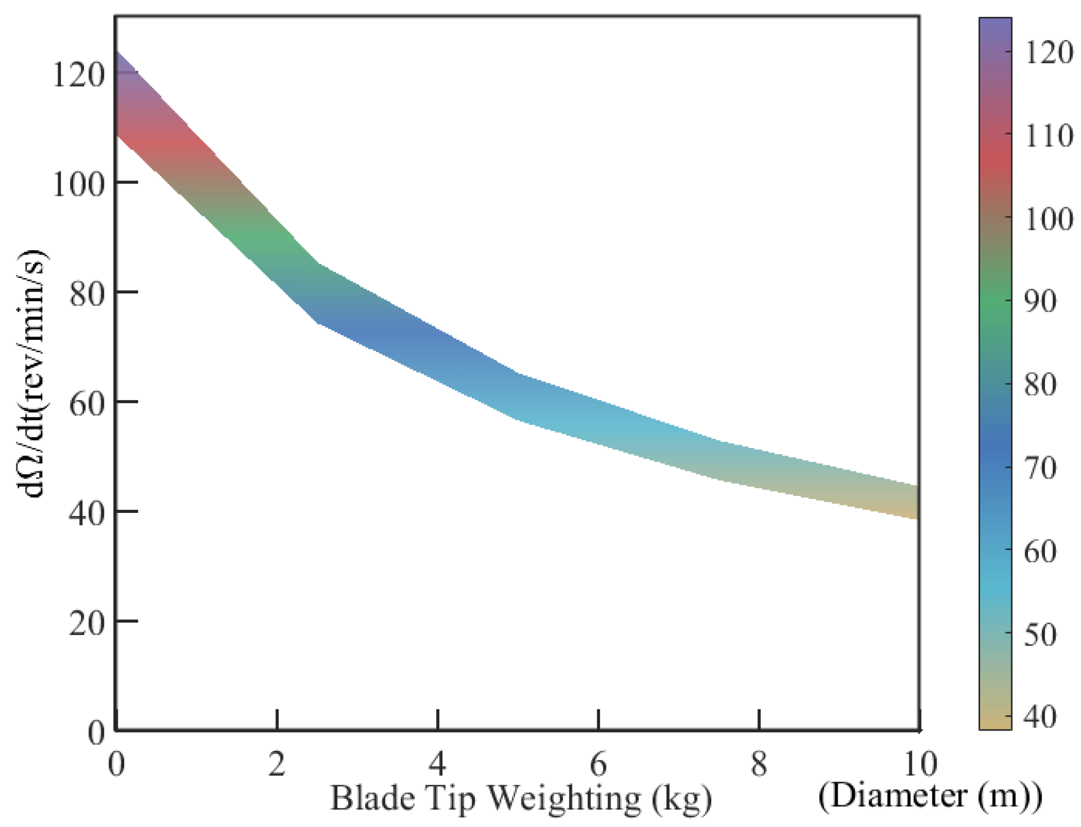
The plot in Figure 23 is projected onto the rotor diameter–decay rate and blade tip weighting–decay rate planes in Figure 24 and Figure 25, respectively. From Figure 24, it can be seen that the rotation speed decay rate is minimally affected by changes in rotor diameter, and so the effect of diameter variations on the decay rate can henceforth be ignored. However, from Figure 25, it can be seen that the speed decay rate is greatly affected by changes in the blade tip weighting: as this weight increases, the speed decay rate decreases with a logarithmic trend, corresponding to better jump-takeoff performance. Once the blade tip weighting has exceeded 8 kg, the curve tends to flatten out, with a slope approaching zero, and the sensitivity to further increases in blade tip weighting becomes small. We select a value for the speed decay rate of 0.707 of its converged value as the optimal design value, i.e., a value of 60 rev/min/s, and at this value we draw a plane parallel to the blade tip weighting–rotor diameter plane and intersecting with the original surface as shown in Figure 23. We thereby obtain an appropriate range for selecting blade tip weightings between 4.5 kg and 6.3 kg.

According to the above results, when the rotor diameter is greater than or equal to 8.5 m and the blade tip weighting is greater than or equal to 5 kg, a significant optimization of maximum jump-takeoff height can be achieved. The blade tip weighting needs to be within the range of 4.5 kg to 6.3 kg for better optimization and to improve the cost-effectiveness of the speed decay rate. Considering the weights of the blades themselves and the strength of the rotor structure, neither the blade tip weighting nor the rotor diameter can be too large. Therefore, a rotor diameter of 8.5 m and a blade tip weighting of 5 kg were selected as optimized values.

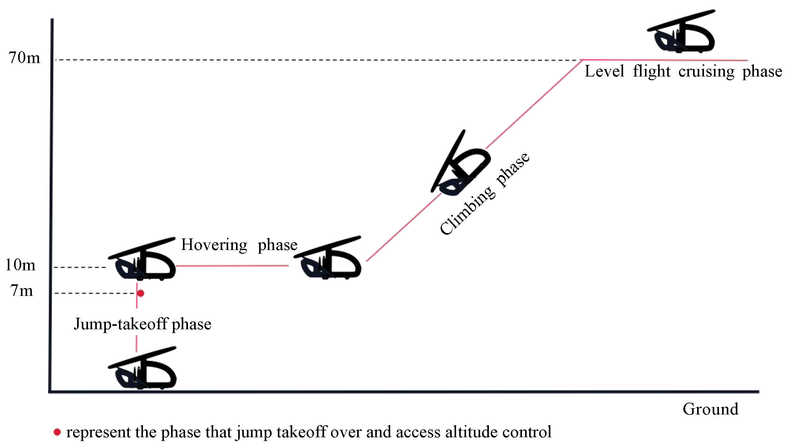
6. Jump-Takeoff and Cruise in Nominal State

This article takes a certain autogyro with a takeoff weight of 450 kg (excluding blade tip weighting) as an example. Based on the data comparison and analysis of results presented above, the following rotor parameters and control variables were determined: an individual blade tip weighting of 5 kg, a pre-rotation speed of 400 rpm, a collective angle at jump-takeoff of 10°, a collective angle at cruising level flight of 2°, and a rotor diameter of 8.5 m.

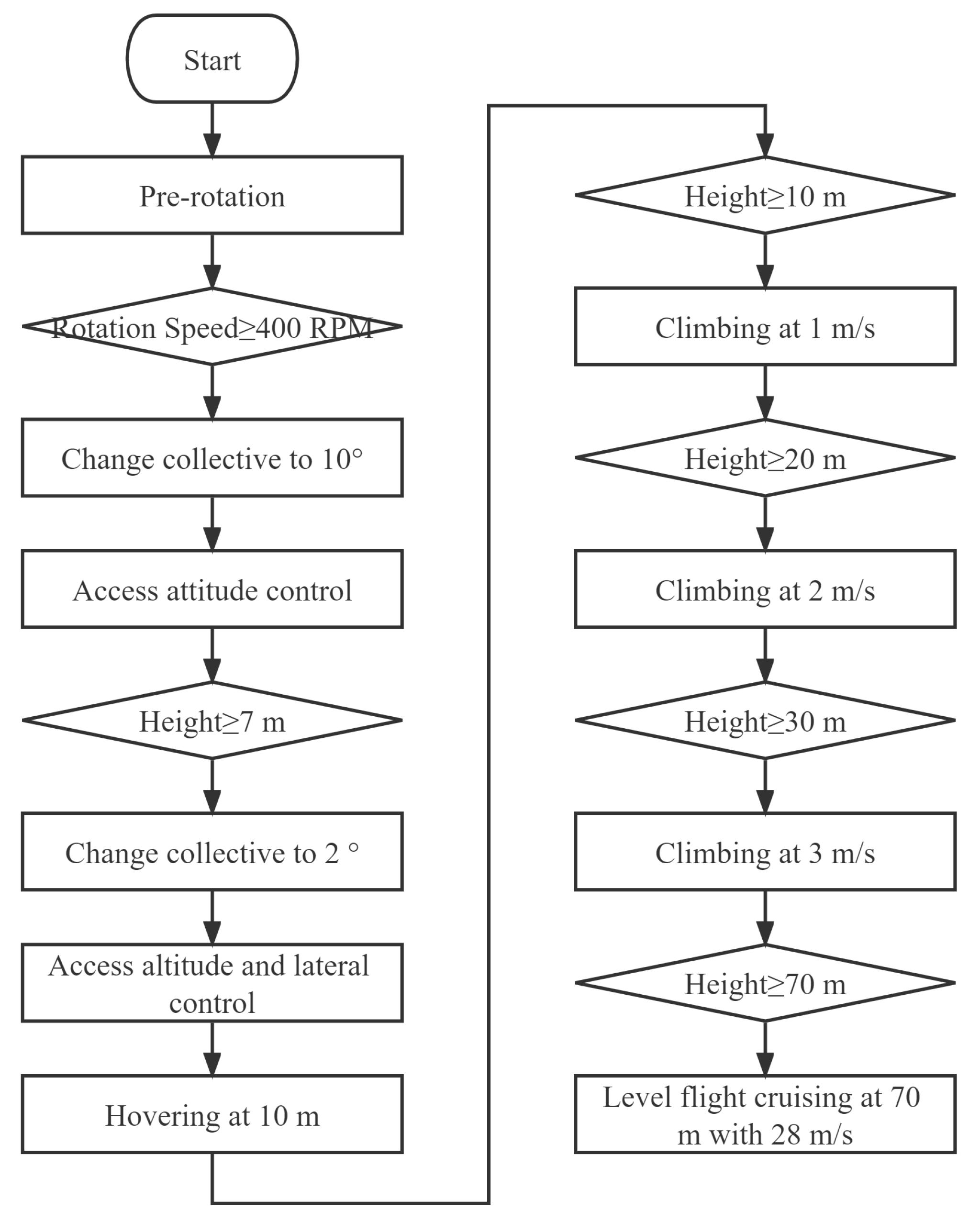
At the beginning of the entire simulation, we started the engine for pre-rotation to achieve a rotation speed of 400 rpm. Then, we changed the collective angle at a rate of 20°/s to 10° while opening the throttle to achieve jump-takeoff. At the same time, we connected the attitude control to stabilize the aircraft. After reaching a specific jump-takeoff height, we lowered the collective angle to the value required for auto-rotation and connected the altitude and lateral controls. We set a specific jump-takeoff height of 10 m and controlled the autogyro to hover at an altitude of 10 m. Based on simulations and engineering experience, we needed to reserve a tolerance limit of 30% to end the jump-takeoff phase ahead of time. Therefore, the altitude and lateral controls were connected when a height of 7 m was reached, so that the autogyro could smoothly enter a hovering state at an altitude of 10 m. Then, we gradually increased the climb rate for a steady climbing process until a predetermined cruising altitude at 70 m was reached, at which the autogyro entered the cruise flight stage. The entire simulation process and flight mission diagram are shown, respectively, in Figure 26 and Figure 27.

Throughout this process, traditional inner-loop/outer-loop separation design control laws were adopted, with traditional PID being used for attitude angle control in both the vertical and horizontal directions. Outer-loop energy total control was used in the vertical direction, while trajectory control was used in the horizontal direction.

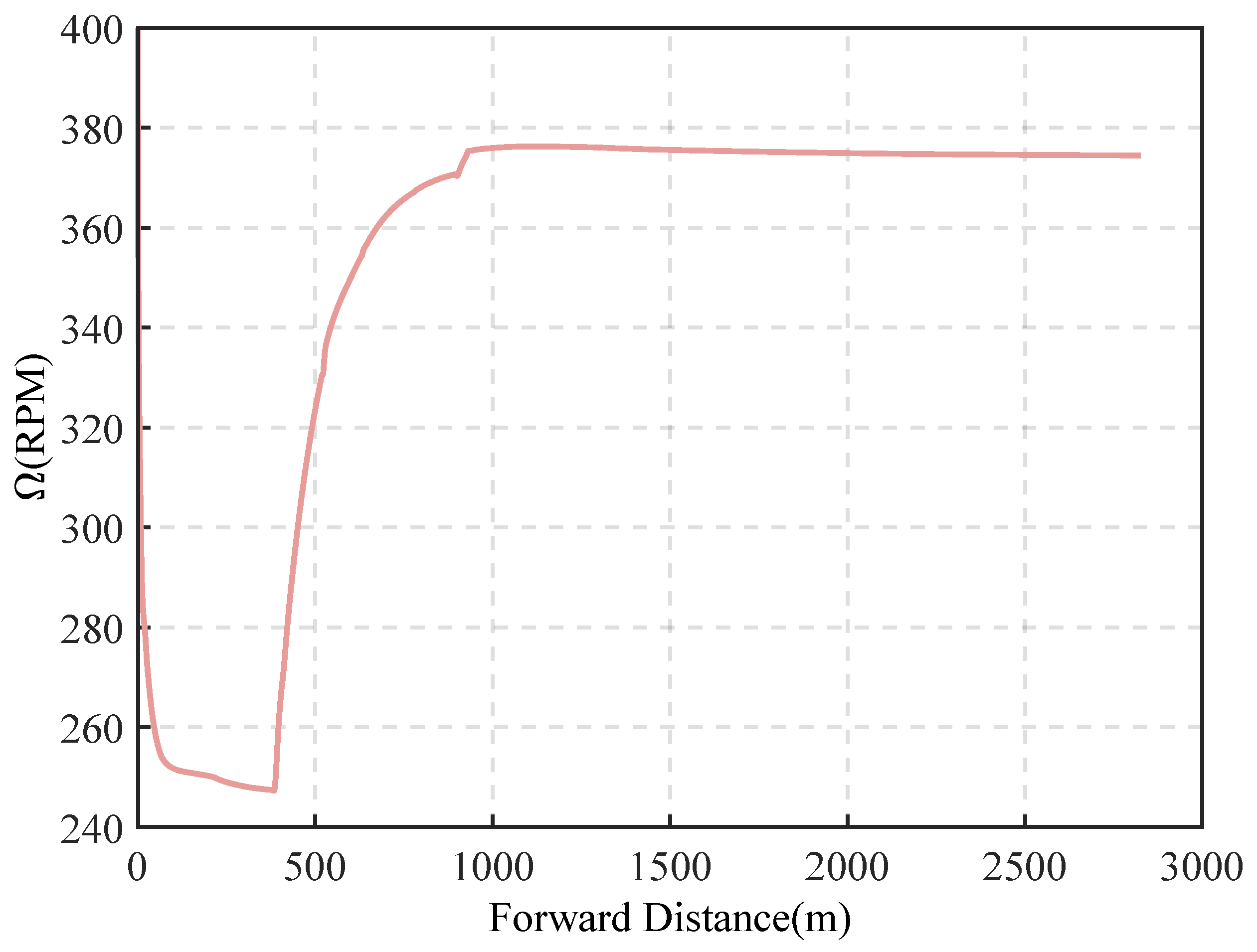
From Figure 28 and Figure 29, it can be seen that at the beginning of the simulation of the jump-takeoff, the rotation speed decreases rapidly. When the collective angle decreases to the angle required for auto-rotation, the rotation speed begins to increase until it stabilizes along with the height and maintains a stable auto-rotation.

After parameter optimization design, the autogyro can achieve a complete jump-takeoff and smoothly transition to the climb and level flight phases, verifying the feasibility of jump-takeoff flight.

7. Conclusions

In this article, high-confidence mathematical modeling of the autogyro designed by Xiamen University has been implemented, a jump-takeoff simulation on the autogyro has been designed and performed, and an in-depth study of its jump-takeoff performance has been conducted. A simplification of blade element theory has been proposed and discussed, and the principles of rotor self-rotation and conditions for jump-takeoff have been studied. The simplified blade element theory presented here enables simple calculations and is easily implemented while retaining high accuracy. Through the proposal of two indicators, namely, jump-takeoff height and rotation speed decay rate, this article has provided theoretical standards for studying jump-takeoff performance.

With regard to engineering applications, on the basis of the YASim dynamics library in FlightGear software, secondary development has been performed in this article to construct a simulation platform for autogyros, and jump-takeoff experiments have been designed and performed. The impact of changes in different control parameters on jump-takeoff performance has been studied. Simulation results show that the collective angle has a significant impact on the jump-takeoff height. On this basis, the optimization of jump-takeoff performance through changes in different rotor parameters has been investigated. It has been found that the optimization of the jump-takeoff height is greatly influenced by the rotor diameter. With the same blade tip weighting, by increasing the rotor diameter, the maximum jump-takeoff height can reach approximately 50 m. The optimization of the rotation speed decay rate is greatly influenced by blade tip weighting. With the same rotor diameter, by increasing blade tip weighting, the minimum rotation speed decay rate can reach approximately 40 rev/min/s. These two data can be observed from Figure 21 and Figure 23. On the basis of these optimized results, combined with engineering experience, we are able to obtain optimal design parameters for rotors. The work described in this article is significant for the future development and optimization of rotor modeling methods and the selection and design of rotor parameters, as well as for the implementation of autogyro jump-takeoff experiments.

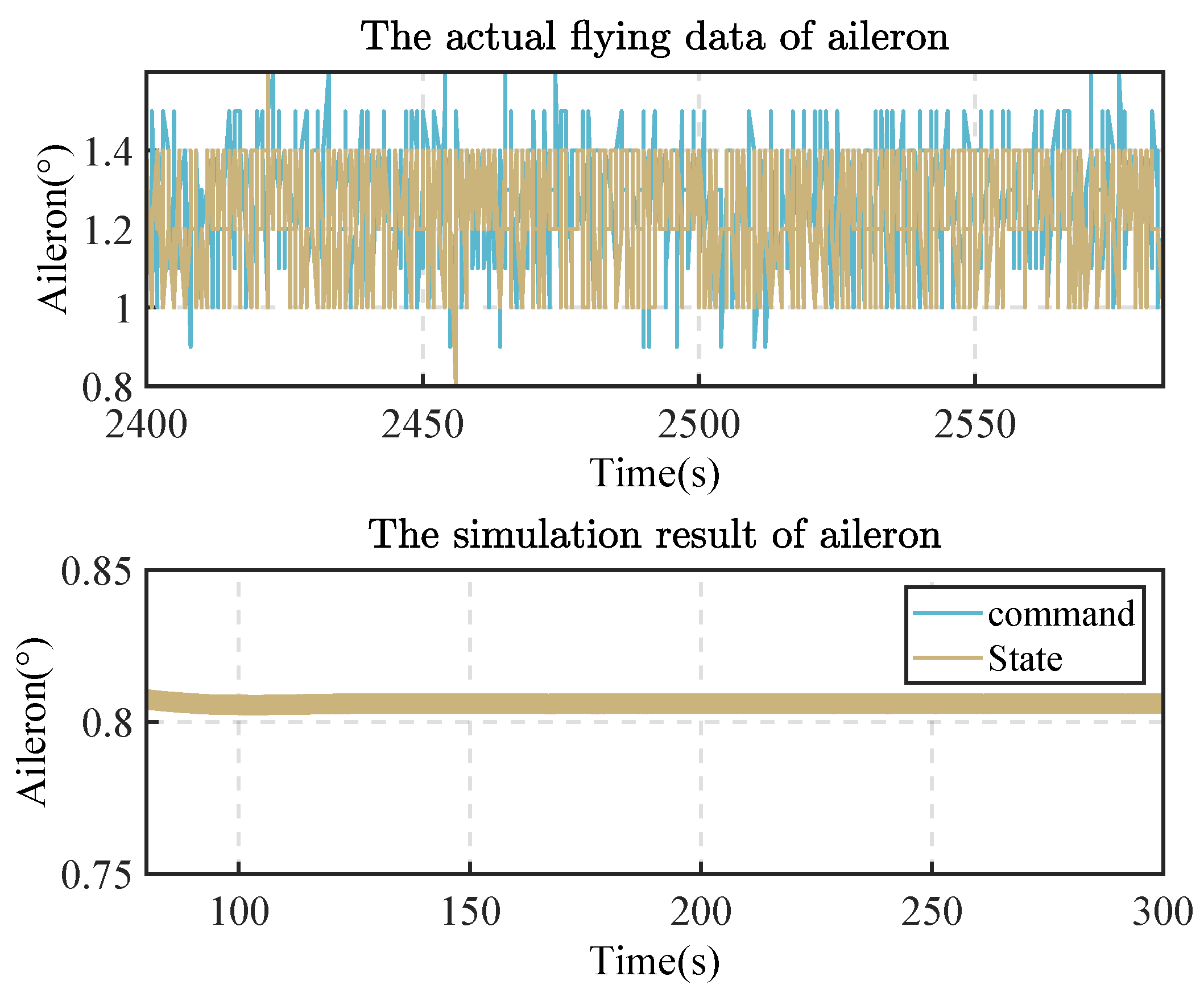
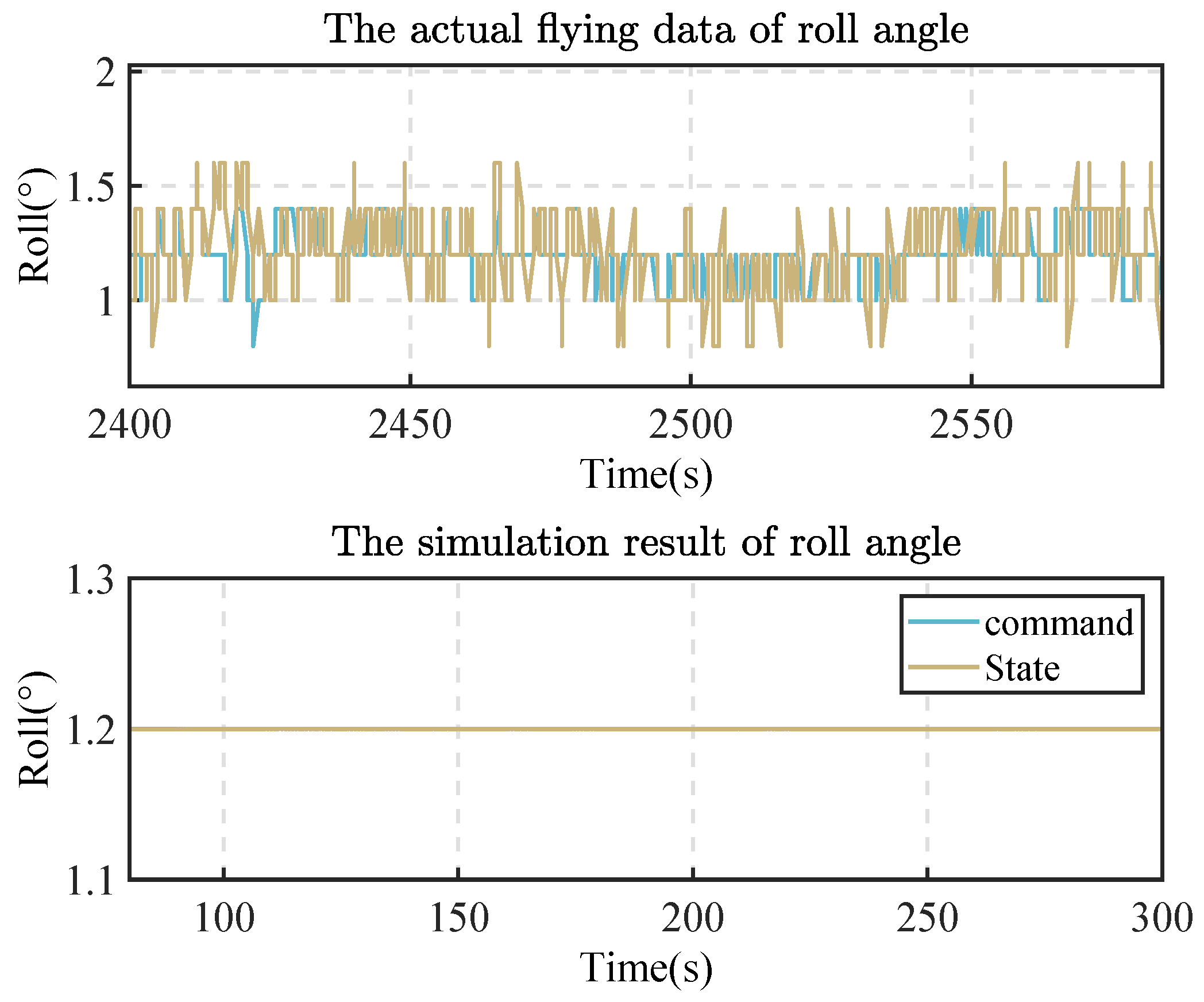
In this article, relatively simple modeling was adopted for the behavior of the autogyro in lateral directions, and there are significant errors between the simulation results and flight data for roll angle, yaw angle, aileron, rudder, etc. In future work, we will aim to improve and extend the modeling of the autogyro to take a more detailed account of movement in lateral directions. Furthermore, it is known that for jump-takeoff, high-inertia rotors can store a greater amount of energy, provide greater lift, and reduce their rotational speed more slowly. Therefore, we will conduct further research on the landing of an autogyro equipped with a high-inertia rotor, with the aim of achieving ultra-short or even vertical landing by changing the collective angle.