A Universal Feature Extractor Based on Self-Supervised Pre-Training for Fault Diagnosis of Rotating Machinery under Limited Data

Abstract

To address the limited data problem in real-world fault diagnosis, previous studies have primarily focused on semi-supervised learning and transfer learning methods. However, these approaches often struggle to obtain the necessary data, failing to fully leverage the potential of easily obtainable unlabeled data from other devices. In light of this, this paper proposes a novel network architecture, named Signal Bootstrap Your Own Latent (SBYOL), which utilizes unlabeled vibration signals to address the challenging issues of variable working conditions, strong noise, and limited data in rotating machinery fault diagnosis. The architecture consists of a self-supervised pre-training-based fault feature recognition network and a diagnosis network based on knowledge transfer. The fault feature recognition network uses ResNet-18 as the backbone network for self-supervised pre-training and transfers the trained fault feature extractor to the target diagnostic object. Additionally, a unique vibration signal data augmentation technique, time–frequency signal transformation (TFST), is proposed specifically for rotating machinery fault diagnosis, which addresses the key task of contrastive learning and achieves high-precision fault diagnosis with very few labeled samples. Experimental results demonstrate that the proposed diagnostic model outperforms other methods in both extremely limited sample and strong noise scenarios and can transfer unlabeled data utilization between similar and even different device types.

1. Introduction

Rotating machinery, such as aero-engines, wind turbines, and gearboxes, is widely used in industry and is prone to various failures under harsh operating conditions such as high temperatures, variable speeds, and heavy loads. Timely fault diagnosis is critical to ensure equipment safety and prevent severe failures [1].

Deep learning [2] has gained increasing attention in the field of fault diagnosis, primarily due to its exceptional feature extraction capability. Convolutional neural networks (CNNs) [3,4,5] are particularly favored for their advantages, including parameter sharing and powerful non-linear feature learning. However, data-driven fault diagnosis models based on deep learning require a large amount of high-quality raw data [6]. Obtaining large labeled datasets is impractical, as operating rotating machinery under fault conditions for extended periods is unrealistic. With only a limited amount of labeled data available, deep learning models struggle to achieve satisfactory fault diagnosis performance.

To address the above problem in fault diagnosis for rotating machinery, researchers have primarily utilized semi-supervised and transfer learning methods. Semi-supervised methods leverage a combination of unlabeled and labeled data to enhance model performance. A method called hybrid classification autoencoder was proposed by Wu et al. [7] to diagnose faults in rotating machinery using features obtained from the autoencoder. A semi-supervised deep sparse autoencoder (SSDSAE) with local and nonlocal information was proposed by Zhao et al. [8] for the intelligent fault diagnosis of rotating machinery. Transfer learning methods, on the other hand, transfer knowledge from a source domain to a target domain to improve diagnostic performance. Li et al. [9] proposed an adversarial transfer learning method based on stacked autoencoders to address fault classification under different operating conditions. Han et al. [10] combine models of joint distributed adaptation and deep networks to facilitate the diagnosis of a new but similar target task.

Although the above-mentioned methods have shown promising results, their applicability is limited to specific scenarios. Semi-supervised methods mainly focus on the case of labeled and unlabeled data from the same diagnostic object, which is difficult to obtain in practical diagnostic tasks. Similarly, transfer learning methods require labeled source domain data to improve diagnostic accuracy [11]. Both methods require computationally expensive training on additional data and target diagnostic data for different diagnostic tasks. Gaining access to a large amount of data from the specific diagnostic object or obtaining labeled data from different diagnostic objects can be challenging. However, unlabeled data from different products is often easily obtainable, raising the question of how to effectively leverage this data resource.

In contrast to the algorithms described above, the self-supervised learning methods explore a new solution that takes full advantage of unlabeled data easily available from different diagnostic objects [12]. Self-supervised learning methods can learn effective signal representations from large-scale unlabeled data, and they have better applicability than semi-supervised learning methods. Moreover, unlike transfer learning methods, self-supervised methods do not require a large amount of labeled source domain data. Furthermore, they do not need repeated training with unlabeled data for each downstream task, so they can be quickly applied to various downstream diagnostic tasks. Many self-supervised learning methods have been developed in the field of computer vision. Some methods deviate from contrastive learning and instead adopt manually designed prediction tasks like image colorization [13], image inpainting [14], image jigsaw puzzle [15], and image super-resolution [16] to learn representations. These alternative approaches have demonstrated their effectiveness. Meanwhile, contrastive learning, as the most advanced self-supervised learning method, performs representation learning by reducing the distance between representations of different augmented views of the same image (“positive pairs”) and increasing the distance between representations of views of different images (“negative pairs”) [17,18]. Contrastive learning has been shown to extract the essential features of the data and provide better representation learning than the methods described above [19,20,21].

However, research on self-supervised learning in fault diagnosis is still limited. Wang et al. [22] employed data augmentation techniques to signals and trained classification models to identify corresponding augmentation methods. Ding et al. [23] proposed self-supervised pre-training via contrast learning (SSPCL), which is based on MoCo [24] and uses momentum contrastive learning for instance-level discrimination, thus enabling feature learning. Wei et al. [25] used SimCLR [20], which first transforms the signal from one-dimensional to two-dimensional using a simple matrix operation, then applies image domain data augmentation methods before converting it back to one-dimensional for representation learning. Yan et al. [26] proposed SMoCo, which is based on MoCo with improved structure and data augmentation techniques. It introduces a novel comparison method and has been successfully applied to bearing fault diagnosis in aero-engines, even with limited data. Shul et al. [27] developed a deep neural network for detecting anomalies in washing machines based on the noise spectra generated during their operation. The main self-supervised task of their architecture is to predict future noise based on past noise. Nie et al. [28] proposed a generalized model based on self-supervised learning and sparse filtering, which employs corresponding labels assigned to signals undergoing different feature transformations for self-supervised learning.

Although the above methods attempt to apply self-supervised learning to fault diagnosis, their applicability is primarily limited to utilizing a large number of unlabeled samples and a small number of labeled samples of the same diagnostic object. Moreover, these methods have not undergone thorough investigation across different noise intensities, operating conditions, sample sizes, and other factors. As a consequence, the lack of a universal feature extractor that can be applied to various types of equipment greatly limits their application scope. The reason for this is that the data augmentation methods utilized in their study were not designed to fully exploit the unique characteristics of vibration signals. In addition, the model architectures employed exhibited several shortcomings, posing challenges to achieving high diagnostic accuracy in complex real-world settings for fault diagnosis purposes. Specifically, Wang and Nie’s method [22,28] only identifies data augmentation categories without instance-level representation learning, limiting its ability to extract robust fault features effectively. In contrast, for contrastive learning methods, Ding’s method [23] employs a time-domain transformation for vibration signal data augmentation but fails to leverage the time- and frequency-domain characteristics simultaneously. Wei’s approach [25] based on SimCLR requires large batch sizes during training, and the data augmentation method it uses is limited to the image domain.

To solve the above problem, this paper proposes a new self-supervised method signal bootstrap your own latent (SBYOL). SBYOL uses two networks including the online network and the target network, which interact and learn from each other, and uses the similarity of the output of the two networks as the loss function. Based on the characteristics of vibration signals, this paper proposes a new contrastive learning data augmentation method, time–frequency signal transformation (TFST). It consists of two parts, time–frequency contrast (TFC) and segment cross contrast (SCC), which greatly helps the model to learn the essential features of the signal. SBYOL can effectively utilize easily accessible unlabeled data with different sources from the object to be diagnosed and learn how to extract the fault characteristics of vibration signals independent from working conditions, noise, and even equipment types. Then, by transferring this capability to various downstream diagnostic tasks, it greatly solves the problems of limited data, complex signals, and strong noise in practical fault diagnosis scenarios and provides a powerful solution for the efficient utilization of industrial big data. The contributions and innovations of this paper are summarized as follows:

(1)

This paper proposes a novel data augmentation method called TFST based on the unique characteristics of vibration signals to address the key points of rotating machinery fault diagnosis, which enables the model to learn signal representations from both the time and frequency domains simultaneously.

(2)

A universal and robust automated feature extractor is constructed in this paper through pre-training on a public parallel gearbox dataset. This feature extractor can achieve excellent diagnostic accuracy using a simple classifier with limited training data, whether it is a private complex planetary gearbox or public planetary gearbox dataset, or even two public bearing products of completely different types.

(3)

The unlabeled pre-training data used by SBYOL are no longer limited to the same diagnostic object but can even be completely different types of equipment, which greatly increases its feasibility in practical tasks.

(4)

Further experiments demonstrate that SBYOL still has excellent accuracy for the target diagnostic object with extremely limited training data and strong noise, has good stability for the unlabeled pre-training dataset with smaller sampling time and data size, outperforms other state-of-the-art methods, and further proves its robustness.

The paper is structured as follows. Section 2 introduces self-supervised learning. Section 3 describes the proposed SBYOL framework. In Section 4, the performance of SBYOL is experimentally verified. Section 5 summarizes the paper and looks at future work.

2. Self-Supervised Learning

For supervised learning, given a labeled dataset $D_L={\left\{x_i,y_i\right\}}_{i=1}^{N_L}$, $x_i$ and $y_i$ are the samples and the corresponding labels in the dataset $D_L$, respectively. A loss function is defined to measure the distance between $y_i$ and the network output ${\widehat{y}}_i$, usually the cross-entropy loss function. The optimization objective of the network is to minimize the cross-entropy loss function, and it performs well on large-scale labeled datasets.

However, labeled data are often difficult to obtain, while self-supervised methods can learn useful representations from unlabeled data. Given an unlabeled dataset $D_U={\left\{x_i\right\}}_{i=1}^{N_U}$, self-supervised methods perform representation learning by constructing a suitable pretext task that minimizes a predefined loss function, which is then transferred to a downstream diagnostic task, thereby improving diagnostic accuracy. Self-supervised learning aims to keep similar samples close and different samples far away [29]. The pretext task is an important concept in self-supervised learning [12], meaning that it solves a task that is not directly needed which is a classification task in the field of fault diagnosis. It defines the task by the attributes found in unlabeled data and thus performs the implementation of unsupervised representation learning. The pretext tasks proposed by previous work mainly focused on performing time-domain transformations on the signal, enabling the model to identify different transformations of the same signal sample and distinguish between different samples.

3. Signal Bootstrap Your Own Latent (SBYOL)

To address the drawback that previous self-supervised learning methods do not make full use of the characteristics of the vibration signals to design the pretext task, we propose a fault diagnosis method based on SBYOL. It has the advantages of strong feature extraction capability, more focus on the signal itself, and weak task correlation, which makes it more suitable for fault diagnosis tasks for different models of equipment or even different types of equipment. This section details the core algorithms of SBYOL, including a novel and efficient method for signal-specific data augmentation, and how unsupervised representation learning can be performed and used for downstream diagnostic tasks.

3.1. Methodology Overview

The purpose of this study is to improve the diagnostic accuracy of the target diagnostic task by making full use of easily available task-independent unlabeled data in cases where there are limited data in practical fault diagnosis. The method allows representation learning on a pre-training dataset without any manual annotation to obtain a feature extractor capable of extracting the essential features of the vibration signal. The learned feature extractor is then transferred to a downstream diagnostic task, thereby improving diagnostic performance. Our approach is divided into three stages, and the flow chart is shown in Figure 1. In the first stage, data collection is performed and divided into an unlabeled pre-training dataset and a labeled target diagnostic dataset, where the pre-training dataset is different from the target diagnostic object. In the second stage, self-supervised learning is used to learn how to extract robust features from unlabeled vibration signal data. In the third stage, the online network encoder obtained by self-supervised learning is transferred to the target diagnosis task and used as a feature extractor with fixed weights. Finally, support vector machine (SVM) is used to classify the features extracted by the feature extractor to obtain the fault diagnosis model. Next, we will describe the second and third learning stages in detail.

3.2. Data Augmentation Based on the Time–Frequency Signal Transformation (TFST)

In contrast to supervised learning, self-supervised learning relies more on the design and optimization of data augmentation methods [20], and it is therefore necessary to design augmentation methods according to the characteristics of the vibration signal. In the actual operation of rotating machinery, there are many diagnostic difficulties, such as variable working conditions and strong noise. If a model can be independent of these factors, then this model can extract essential features from the signal, and therefore, transferring this capability to fault diagnosis tasks can greatly improve diagnostic performance. In contrast to previous approaches that focus solely on morphological changes and time-varying operations, this paper introduces a novel set of pretext tasks based on signal transformations, specifically leveraging the time–frequency characteristics of the signal. Notably, the innovative TFST method is proposed, significantly enhancing the model’s capability for representation learning. Details of how these methods transform a given vibration signal $x=\left[x_1,x_2,\cdots ,x_N\right]$ are described below:

(1)

Normalize, as shown in Figure 2a. As there are differences in the measurement ranges of different sensors, this strategy normalizes the signals to a uniform measurement range, and in addition, it optimizes the convergence of the model. The formula is as follows:

$$\tilde{x}=-1+2\times \frac{x-x_{\mathrm{m}\mathrm{i}\mathrm{n}}}{x_{\mathrm{m}\mathrm{a}\mathrm{x}}-x_{\mathrm{m}\mathrm{i}\mathrm{n}}}$$

(1)

(2)

AddGaussian, as shown in Figure 2b. As noise is inevitable in the actual operating environment of the device, this strategy improves the model’s immunity to noise by randomly adding Gaussian noise to the input signal, which is formulated as follows:

$$\tilde{x}=x+n,n~N\left(0,{\sigma }_n\right)$$

(2)

where $n$ is generated by Gaussian distribution $N\left(0,{\sigma }_n\right)$.

(3)

Scale, as shown in Figure 2c. Since the equipment is loaded to different degrees in the actual operating environment, the sensitivity of the model to signals of different amplitudes can be improved by changing the amplitude of the signals, thus enabling the diagnosis of variable working condition faults. The strategy multiplies the input signal randomly by a factor s, which is calculated as follows:

$$\tilde{x}=x\times s,s~N\left(1,{\sigma }_s\right)$$

(3)

where $s$ is generated by the Gaussian distribution $N\left(1,{\sigma }_s\right)$.

(4)

Stretch, as shown in Figure 2d. In response to the existence of different working conditions in the operation of the equipment, the signal is resampled, and its length is converted to the original length in $s~N\left(1,{\sigma }_s\right)$ times, simulating the speed variation of different operating conditions. Finally, equal lengths are ensured by zeroing and truncation.

(5)

Crop, as shown in Figure 2e. For the problem of missing data during fault diagnosis, this strategy randomly overwrites some signals with the following equation.

$$\tilde{x}=x\times mask$$

(4)

where the mask is a binary sequence with a random subsequence of zeros.

(6)

Flip, as shown in Figure 2f. The vibration signal usually oscillates up and down with an average value of zero. To improve the model from the effects of positive and negative signals, the strategy simulates this variation by randomly flipping the signal with the following equation.

$$\tilde{x}=-x$$

(5)

(7)

Time–frequency signal transformation (TFST)

The proposed time–frequency signal transformation (TFST), illustrated in Figure 3, integrates both segment cross contrast (SCC) and time–frequency contrast (TFC) techniques. This combination enables the extraction of features from both the time domain and the frequency domain simultaneously. Moreover, it retains the prior information from the time-domain signal interception, thereby greatly improving the ability of representation learning for contrastive learning. Next, we will introduce the intuition and principles of SCC and TFC in detail.

The SCC is shown on the left side of Figure 3. During signal acquisition, the state of the device does not change much over a short period, thus allowing it to be considered as the same state. After sampling, a long signal is obtained, and it is necessary to segment the long signal to obtain multiple signal instances that can be used as training data for the model. However, traditional contrastive learning only considers instances as individual classes and disregards that different instances segmented from the same long signal belong to the same class. To address this issue, we propose a strategy of comparing signal instances obtained by intercepting the same long-sampled signal with each other. This approach can increase the prior knowledge of model training, facilitate the identification and aggregation of similar samples during the representation learning process, and enhance the model’s ability to withstand time disturbances. Specifically, two different signals $x_1$ and $x_2$ are randomly selected from the same long-sampled signal interception set. They undergo a series of signal transformations, respectively, and finally, their representations are made as similar as possible.

The TFC, depicted on the right side of Figure 3, leverages both time-domain and frequency-domain features of vibration signals, which are commonly extracted as fault features, to enable effective analysis of such signals. In this paper, the original time-domain signal is compared with its fast Fourier transform (FFT) counterpart, allowing signal representation extraction from two dimensions. To achieve this, a series of data augmentation methods are applied to the time-domain signal, including Normalize, AddGaussian, Scale, Stretch, Crop, and Flip, which is referred to as time domain transformation (TDT). Additionally, the FFT, Normalize, and AddGaussian are used as data augmentation methods to generate the frequency-domain feature, referred to as frequency-domain augmentation (FDT). The overall strategy involves comparing the original signal after TDT transform with the original signal after FDT transform, to minimize the distance between the two representations.

Therefore, the overall process of TFST is that, given a long-sampled signal from which two segments of the signal $x_1$ and $x_2$ are randomly intercepted, the TDT transform of $x_1$ and the FDT transform of $x_2$ are performed, respectively, and finally, their representations are made as close as possible.

3.3. Self-Supervised Signal Representation Learning

In the self-supervised signal representation learning stage, SBYOL uses two neural networks for training: the online network and the target network, as shown in Figure 4. SBYOL obtains new and continuously enhanced representations by enabling the online network to predict the representations of the target network. This iterative process results in a sequence of representations that become increasingly refined. After completing the training, only the encoder $f_{\theta }$ of the online network is retained for use in downstream tasks.

The online network consists of a set of weights $\theta$ and includes three components: an encoder $f_{\theta }$, a projector $g_{\theta }$, and a predictor $q_{\theta }$. While the original self-supervised learning methods with a deeper ResNet encoder were designed for computer vision tasks, fault diagnosis of rotating machinery is simpler compared to representation learning of images, and it can be difficult to achieve convergence with high computational complexity when using a deep network architecture. Therefore, this paper employs the encoder with a lighter architecture ResNet-18 [30], to reduce the computational complexity. Specifically, ResNet-18 consists of 18 layers in total, including 16 1D convolutional layers and 2 fully connected layers. The initial convolutional layer performs a 1 × 7 convolution with stride 2, followed by a max pooling layer. Then, four sets of residual blocks are stacked, each containing two 1D convolutional layers with 1 × 3 filters. The number of filters in each block gradually increases from 64 to 512, capturing more complex patterns as the spatial dimension reduces. Both the projector and the predictor are multilayer perceptrons (MLP), with the same output dimensions. To ensure stable training, batch normalization (BN) [31] is incorporated into the projector and predictor.

The target network has the same structure as the encoder and projector of the online network but uses different weights $\xi$. During training, the online network predicts the targets generated by the target network, and the predictor in the online network greatly increases flexibility, as it allows for different features in the online and target networks to be matched by the predictor, thereby improving representation learning. To prevent the target network parameters $\xi$ from updating during training, stop-gradient (sg) is employed, and the target network is updated via exponential moving average using the online network parameter $\theta$. This approach ensures that the two networks have different parameters so that when the online network regresses the signal features, the targets are distinct, and feature dispersion is preserved. Given the update parameter $\tau \in \left[0,1\right)$, after each epoch, it updates the target network as follows.

$$\xi \leftarrow \tau \xi +\left(1-\tau \right)\theta$$

(6)

To generate the pretext task for self-supervised learning in SBYOL, two random samples ($x_1$ and $x_2$) are extracted from a long signal, and data augmentation is applied to each of them using two distributions (TDT and FDT) to create two corresponding augmented time series ($v$ and $v^{\prime }$). For the first augmented sequence $v$, the online network outputs the feature $z_{\theta }=g_{\theta }\left(f_{\theta }\right(v\left)\right)$ and then uses the predictor to predict $z_{\theta }$ to obtain $q_{\theta }\left(z_{\theta }\right)$. For the second augmentation sequence $v^{\prime }$, the target network outputs $z_{\xi }^{\prime }=g_{\xi }\left(f_{\xi }\right(v^{\prime }\left)\right)$. Additionally, to prevent the scale of features from approaching zero and avoid model collapse, both $q_{\theta }\left(z_{\theta }\right)$ and $z_{\xi }^{\prime }$ are normalized by $l_2$, resulting in $\overline{q_{\theta }}\left(z_{\theta }\right)=q_{\theta }\left(z_{\theta }\right)/{‖q_{\theta }\left(z_{\theta }\right)‖}_2$ and ${\overline{z}}_{\xi }^{\prime }=z_{\xi }^{\prime }/{∥z_{\xi }^{\prime }∥}_2$. This normalization ensures that the model does not learn shortcuts and that the features remain well-scaled. Training is performed by minimizing the mean square error between the normalized online network prediction and the target network projection.

$${\mathcal{L}}_{\theta ,\xi }\triangleq {‖\overline{q_{\theta }}\left(z_{\theta }\right)-\overline{z_{\xi }}‖}_2^2=2-2\cdot \frac{⟨q_{\theta }\left(z_{\theta }\right),z_{\xi }^{\prime }⟩}{{‖q_{\theta }\left(z_{\theta }\right)‖}_2\cdot {‖z_{\xi }^{\prime }‖}_2}$$

(7)

The SBYOL network gets the symmetric loss function ${\tilde{\mathcal{L}}}_{\theta ,\xi }$ of ${\mathcal{L}}_{\theta ,\xi }$ by sending $v^{\prime }$ to the online network and $v$ to the target network. Finally, the network updates the online network ${\theta }_q$ by minimizing the loss ${\mathcal{L}}_{\theta ,\xi }^{\mathrm{S}\mathrm{B}\mathrm{Y}\mathrm{O}\mathrm{L}}$:

$${\mathcal{L}}_{\theta ,\xi }^{\mathrm{S}\mathrm{B}\mathrm{Y}\mathrm{O}\mathrm{L}}={\mathcal{L}}_{\theta ,\xi }+{\tilde{\mathcal{L}}}_{\theta ,\xi }$$

(8)

The detailed training algorithm for self-supervised signal representation learning is shown in Algorithm 1.

Algorithm 1: Self-Supervised Signal Representation Learning

Input: Structure of $f_{\theta }$, $g_{\theta }$, $q_{\theta }$, $f_{\xi }$, $g_{\xi }$, initial online network parameters $\theta$, initial target network parameters $\xi$, update parameter $\tau$, batch size $M$, learning rate $\eta$, optimization step $N$, distributions of transformations $TDT$, $FDT$, set of signals $D$ for $n=1$ to $N$ do    $\mathrm{B}\mathrm{a}\mathrm{t}\mathrm{c}\mathrm{h}\leftarrow {\left\{(x_{1i},x_{2i})\sim D\right\}}_{i=1}^{\mathrm{M}}$    for $(x_{1i},x_{2i})\in \mathrm{B}\mathrm{a}\mathrm{t}\mathrm{c}\mathrm{h}$ do       $t\in TDT$ and $t^{\prime }\in FDT$       $z_1\leftarrow {g_{\theta }(f}_{\theta }\left(t\left(x_{1i}\right)\right))$ and $z_1^{\prime }\leftarrow {g_{\xi }(f}_{\xi }\left(t^{\prime }\left(x_{2i}\right)\right))$       $z_2\leftarrow {g_{\theta }(f}_{\theta }\left(t\left(x_{2i}\right)\right))$ and $z_2^{\prime }\leftarrow {g_{\xi }(f}_{\xi }\left(t^{\prime }\left(x_{1i}\right)\right))$       $l_i\leftarrow -2\times (\frac{⟨q_{\theta }\left(z_1\right),z_1^{\prime }⟩}{{‖q_{\theta }\left(z_1\right)‖}_2\cdot {‖z_1^{\prime }‖}_2}+\frac{⟨q_{\theta }\left(z_2\right),z_2^{\prime }⟩}{{‖q_{\theta }\left(z_2\right)‖}_2\cdot {‖z_2^{\prime }‖}_2})$    end //Back-propagation    $\theta \leftarrow \theta -\eta \cdot \frac{\partial \frac{1}{M}\sum _{i=1}^{\mathrm{M}}{l}_i}{\theta }$ //Exponential moving average without back-propagation    $\xi \leftarrow \tau \xi +\left(1-\tau \right)\theta$ end Output: Online network encoder $f_{\theta }$

3.4. Fault Diagnosis Based on Knowledge Transfer

After training, the convolutional layers of the online network encoder are extracted and used for feature extraction in the downstream tasks. It is worth noting that the weights of the convolutional layers are kept fixed to handle downstream complex tasks under challenging conditions, such as limited data and significant noise. This strategy helps maintain the robustness of the model, preventing bias caused by overfitting with small training sets. Additionally, by keeping the weights fixed, the model can be readily used for downstream diagnostic tasks without requiring any additional training. This approach not only ensures efficiency but also allows for faster deployment of the model in practical applications. Since SVM is the classifier with the largest interval in the feature space and has stronger robustness in problems with limited data, this paper uses SVM to classify the extracted features to build the final fault diagnosis model.

4. Experiment Validation

Due to the small number of scenarios in which planetary gearboxes are used, they often have limited data problems, and there are almost no public data. In addition, compared to parallel gearboxes, their structure is more complex, and their signal composition is relatively complicated, making their diagnosis a difficult task. In contrast, parallel gearbox data are relatively easier to obtain, so in this paper, the unlabeled public University of Connecticut (UoC) parallel gearbox dataset [32,33] is used as the pre-training dataset. To verify the effectiveness and superiority of SBYOL, SBYOL first performs self-supervised signal representation learning on the unlabeled pre-training dataset; then, the learned feature extractor is transferred to the private Drivetrain Prognostics Simulator (DPS) planetary gearbox under limited data conditions and uses the public SEU planetary gearbox dataset [34] for further validation. To further validate the robustness and generalizability of SBYOL, this paper further increases the difficulty by using the trained feature extractors for fault diagnosis in limited data cases on two public datasets, the Paderborn University (PU) bearing dataset [35] and the Polytechnic University of Turin (PUT) aero-engine bearing dataset [36], which are characterized by completely different types of equipment than the pre-training parallel gearbox data. The data distribution between the pre-training dataset and the target diagnostic object is significantly different, and thus, it can be effectively verified that SBYOL learns a universal feature extractor that can efficiently diagnose different types of rotating machines under limited data.

4.1. Self-Supervised on the Unlabeled Pre-Training Parallel Gearbox Dataset

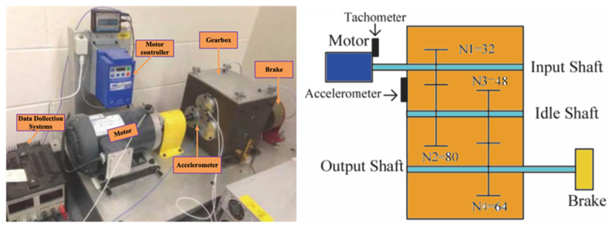
In this paper, the UoC parallel gearbox fault dataset [32,33] provided by the University of Connecticut is used as the unlabeled pre-training dataset, which is the most difficult public dataset with different failure modes and degrees [37]. The dataset is collected at 20 kHz and introduces nine different gear states for pinions on the input shaft, including health condition, missing tooth, root crack, spalling, and chipping tip with five different levels of severity, and they are labeled from 0 to 8, respectively. The test rig is shown in Figure 5.

Our method selects the raw vibration signal as the input data without any signal pre-processing, and 4096 was chosen as the sample length to contain enough information. In addition, the overlap length between two adjacent samples is 3036 when using the sliding segmentation method to obtain training samples, thus greatly increasing the size of the pre-training dataset. This is also a data augmentation strategy that increases the consideration of temporal offset; however, the information capacity of the dataset does not increase. To mimic the phenomenon of intercepting a signal from a long sampling signal, this paper treats approximately 9.43 s of data as a long sampling signal with 175 samples intercepted from a single sampling signal, and finally, an unlabeled pre-training dataset containing nine classes with 350 samples per class is obtained.

Since this paper uses both time-domain and frequency-domain data for learning and even contains learning between different samples, the data distribution between them is quite different; the learning task is also more complicated, and 0.1 is chosen as the initial learning rate. In this study, we adopted the numerical values of Momentum and Weight decay from [24], while the update parameter τ was derived from [18]. Regarding data augmentation methods, using larger values can enhance the model’s noise resistance capability. However, it is essential to strike a balance and avoid excessive values that may lead to information overload. The specific hyperparameter values are shown in

Table 1. Hyperparameter setting.

Hyperparameter	Value	Data Augmentation	Value
Batch size	64	Normalization	/
Optimizer	Stochastic gradient descent (SGD)	AddGaussian	Noise coefficient ${\sigma }_n=0.05$
Learning rate	0.1	Scale	Scale coefficient ${\sigma }_s=0.05$
Momentum	0.9	Stretch	Stretch coefficient ${\sigma }_s=0.3$
Weight decay	1 × 10−4	Crop	Crop length = 100
Epochs	3000	Flip	/
Learning rate schedule	Cosine
Update parameter $\tau$	0.996

. It is worth noting that all the data augmentation methods except TFC and SCC are implemented with a probability of 0.5 to increase the complexity of the pretext task. The learning rate is updated by the cosine learning rate scheduler with the following formula.

$${\eta }_t=\frac{1}{2}(1+cos(\frac{t\pi }{T}\left)\right)\eta$$

(9)

where $\eta$ is the initial learning rate, ${\eta }_t$ is the current learning rate, $T$ is the maximum number of epochs, and $t$ is the current epoch.

The model has a parameter count of 8.48 million and achieves a computational efficiency of 2.81 billion floating-point operations per second (GFLOPs). The experimental environment was PyTorch 1.11 under Windows 11, running on a computer with the following configuration: i5-12400F, NVIDIA RTX 3060, 16 GB RAM. The changes in the loss values during the training process are shown in Figure 6, from which it can be found that the loss values become smooth in the later stages of training indicating that the model has reached the fitting state, and the total training time is about 6.5 h.

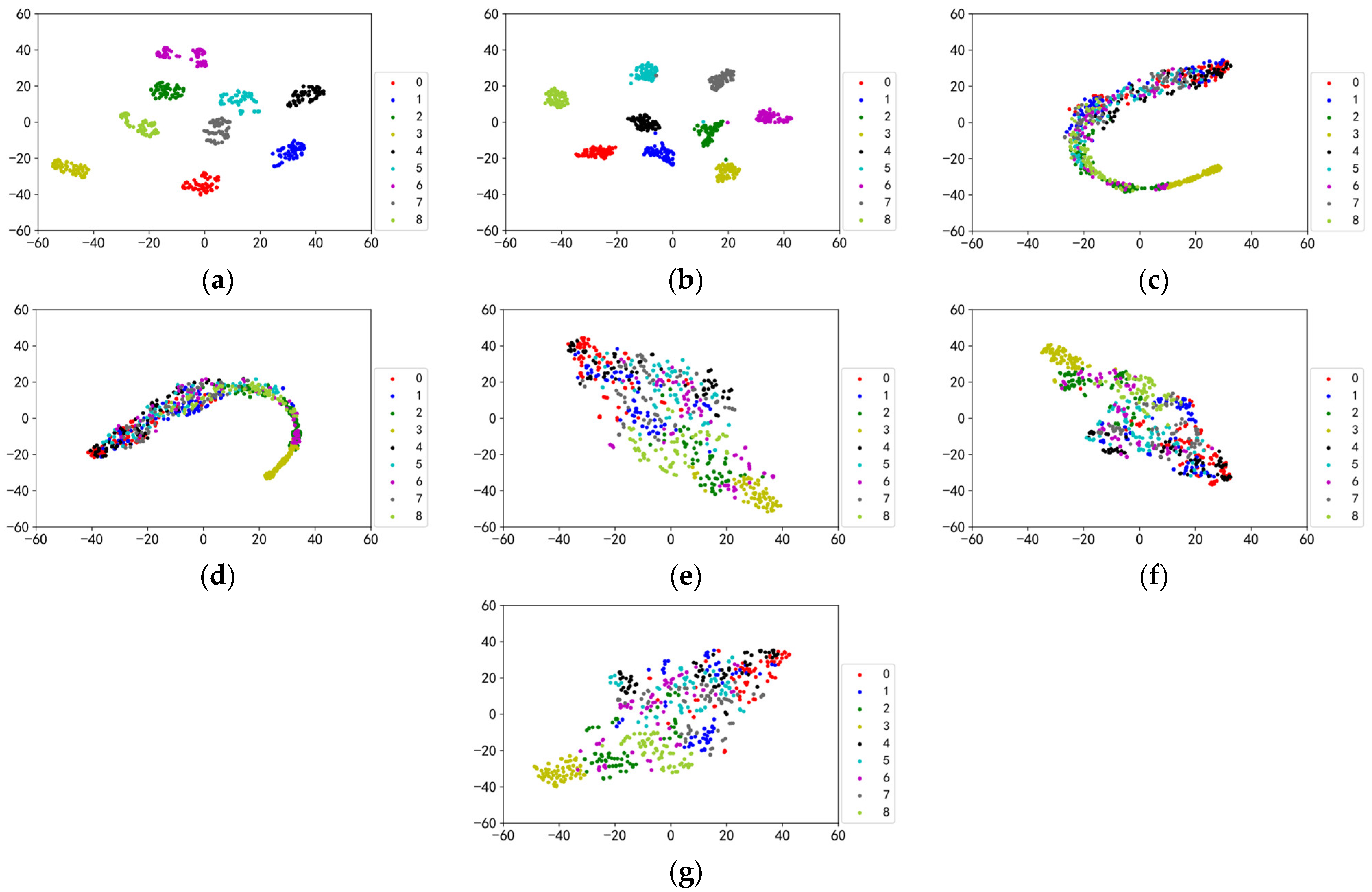
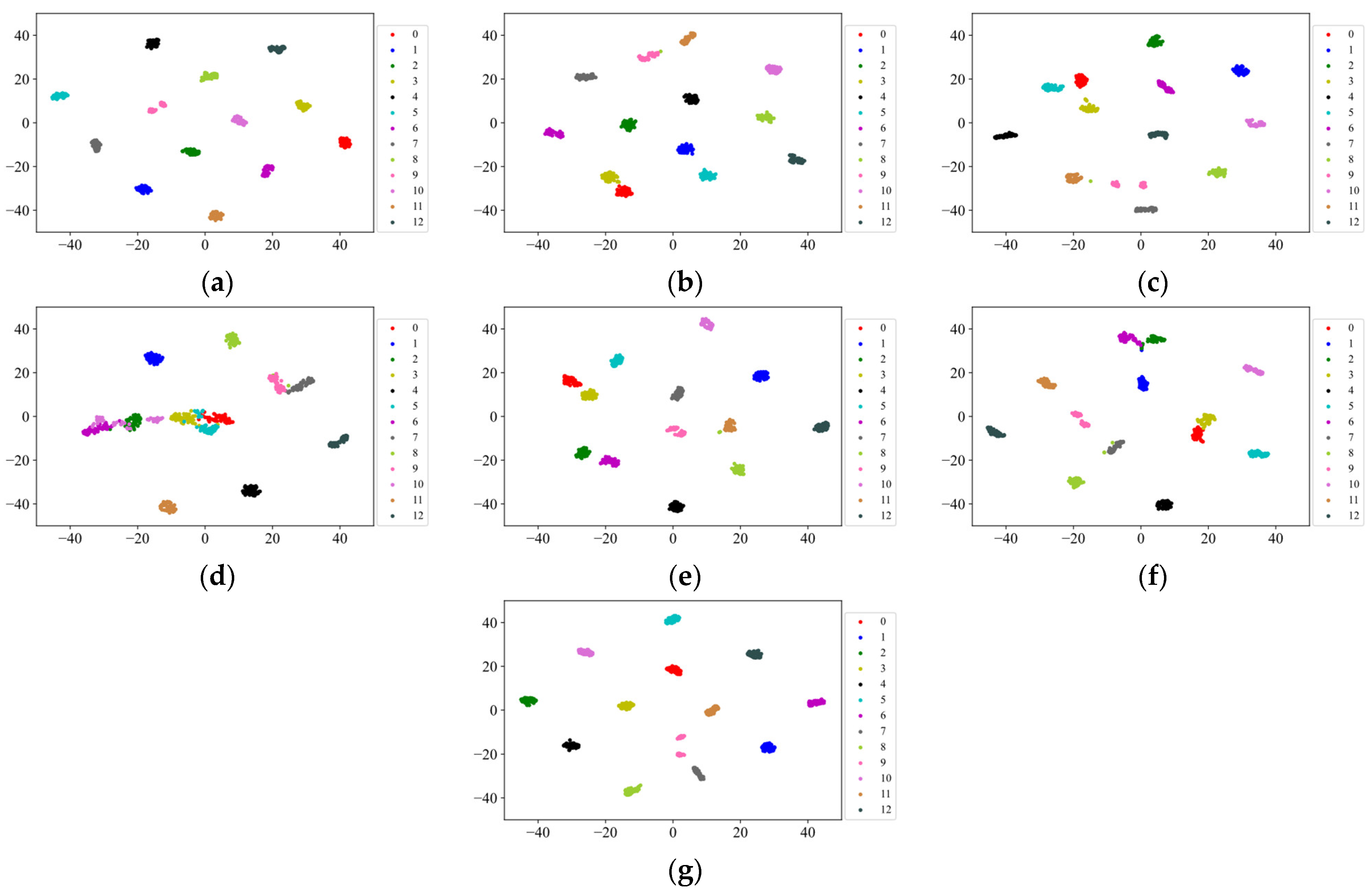
As a comparison, other self-supervised learning methods, SimSiam [39], SimCLR, BYOL, MoCo, and SMoCo, are also used in this paper for self-supervised pre-training on the unlabeled pre-training dataset. In addition, to further demonstrate the powerful performance of SBYOL, this paper also uses the labeled pre-training dataset for supervised pre-training, called Labeled Pre-Training. To exclude the influence of other factors, the backbone network of all methods is ResNet-18, which is trained using time-domain signals. After training, the feature extractors of all methods, i.e., the convolutional layers of ResNet-18, are used to extract features from a portion of the pre-training dataset and downscale it to two dimensions using T-SNE for visualization; the results are shown in Figure 7. Our method, SBYOL, achieves very good results with inter-class separation and intra-class aggregation, reaching the results of Labeled Pre-Training. In the face of such complex data, other self-supervised methods not only have no clustering within the class but also do not have an effective separation between classes, and only SMoCo performs better roughly achieving clustering of three classes of samples.

4.2. Application on Planetary Gearbox from Private DPS Test Rig

In this section, the pre-trained SBYOL feature extractor is used to perform fault diagnosis on the planetary gear from our Drivetrain Prognostics Simulator (DPS) test rig, which is characterized by a different device with different failure levels, different failure modes, and different working conditions compared with the unlabeled pre-training dataset.

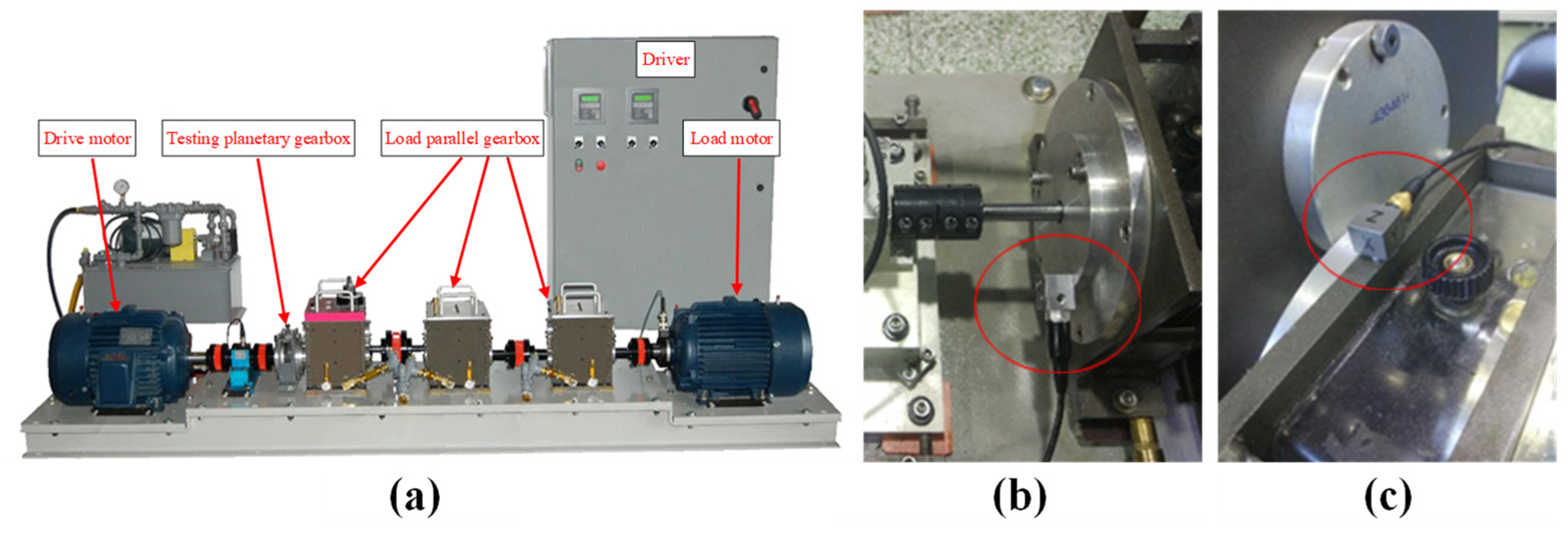
The Drivetrain Prognostics Simulator is shown in Figure 8a which is manufactured by Spectra Quest, U.S.A. The test rig is mainly composed of the following parts: driver (control cabinet), lubrication system, drive motor, testing planetary gearbox, three load parallel gearboxes, load motor and supporting torque transducer and force transducer, etc. The testing planetary gearbox of this test rig is a one-stage drive, compared with the parallel gearbox, it has a more complex structure, including the central fixed sun wheel, planetary frame, and gear ring, and also includes four planetary wheels that change with the sun wheel rotation center at all times; the signal composition is very complex, and therefore, fault diagnosis is a more difficult task. During the data collection, we collected gear data for five states, including wear, broken teeth, missing teeth, root crack, and healthy, where the four failure modes of the gears are shown in Figure 9.

Two vibration sensors were used in the experiment, one is an end cap sensor shown in Figure 8b, and the other is a three-phase sensor mounted on the box shown in Figure 8c. The sampling frequency is 12.8 kHz. Due to the complex transmission path of the fault signal through the gear, shaft, bearing, and end cup to reach the box, the signal collected by the box vibration sensor will become weak. To verify the effectiveness of SBYOL in extreme cases, this paper selects the Z-axis box vibration signal, which is more in line with the complex environment in the actual diagnosis task. To reflect the extremely limited data situation in the actual diagnosis process, only 5 samples per class are used in the training set, and 50 samples per class are used in the testing set. The details of the DPS gear dataset are shown in

Table 2. Labeled DPS gear dataset.

Damaged Element	Rotation Speed (Hz)	Load (Nm)	Training Samples	Testing Samples	Label
Healthy	60	1.2	5	50	0
Healthy	40	0.6	5	50	1
Wear	60	1.2	5	50	2
Wear	40	0.6	5	50	3
Broken teeth	60	1.2	5	50	4
Broken teeth	40	0.6	5	50	5
Missing teeth	60	1.2	5	50	6
Missing teeth	40	0.6	5	50	7
Root crack	60	1.2	5	50	8
Root crack	40	0.6	5	50	9

, which contains two working conditions, and the length of each sample is still 4096.

To demonstrate the performance of the feature extractors learned on the unlabeled pre-training dataset, this paper uses the pre-trained feature extractors to perform feature extraction on the DPS testing set without any training and visualizes the results using T-SNE as shown in Figure 10. The features extracted by SBYOL without any adaptation of the target diagnostic object can be segmented between different classes and aggregated of the same class, far surpassing other self-supervised methods, and even Labeled Pre-Training. SMoCo also adopts the way of extracting features from the time and frequency domains simultaneously, and its feature extraction effect on the testing set data is relatively good, but it lacks unique SCC, and compared to SBYOL, labels 4, 8, and 9 are too close, so it is more prone to errors with very few training data.

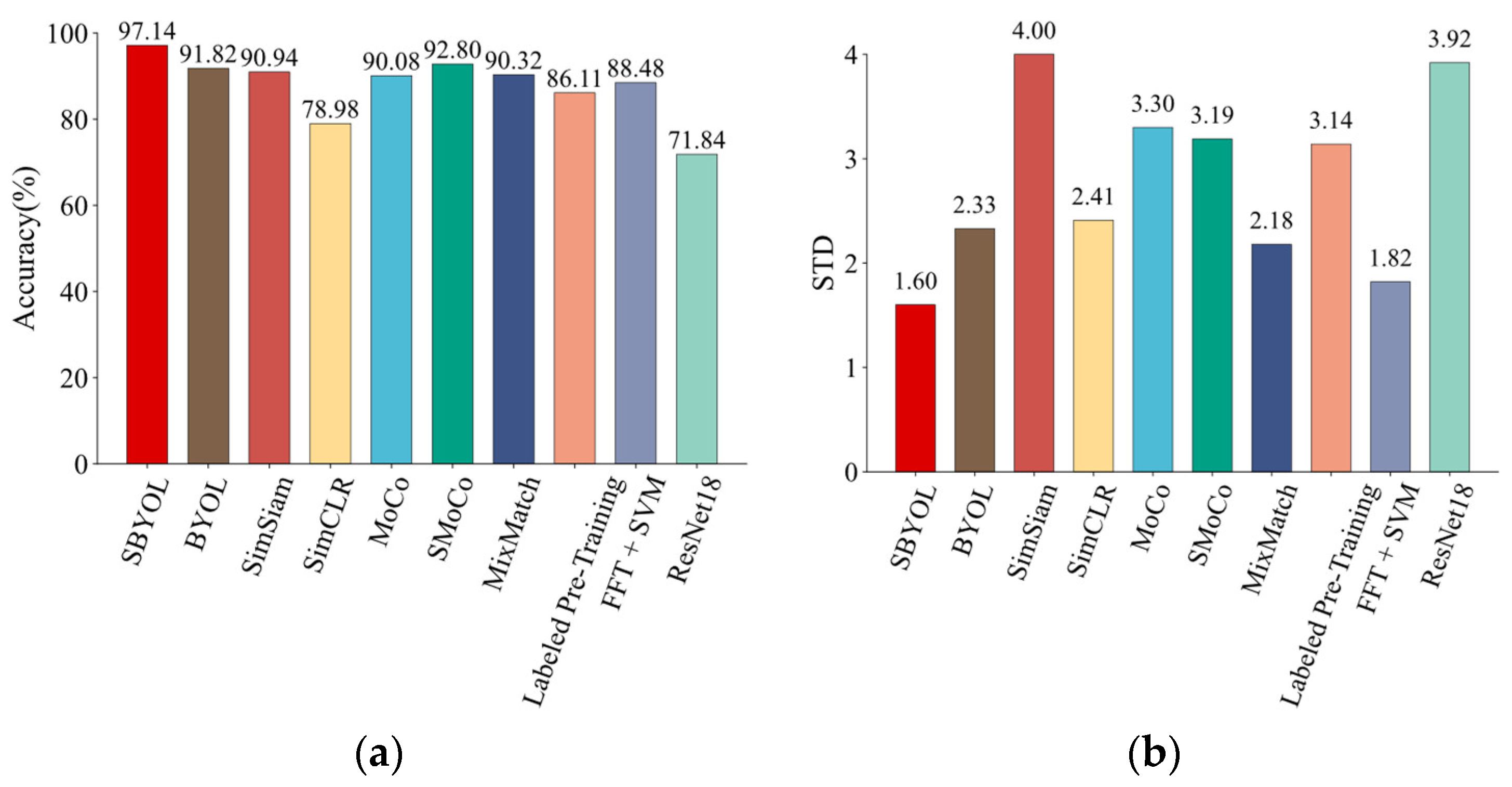
To fully demonstrate the superiority of our method in the target diagnosis task, we also added MixMatch [40], ResNet-18, and FFT + SVM as comparisons for the target diagnostic dataset. Among them, MixMatch is a powerful semi-supervised method that uses both an unlabeled pre-training dataset and labeled target diagnostic training set for training. ResNet-18 uses only the targeted diagnostic training set for supervised learning and does not use the unlabeled pre-training dataset as the baseline model. FFT + SVM is a classical and effective method for fault diagnosis under limited data. The method first performs FFT transformation on the original signal and then classifies the FFT transformed features using SVM. The diagnostic accuracy of each method is shown in

Table 3. Comparison results on DPS gear dataset.

Method	Accuracy (%)	Time (s)
SBYOL	97.14 ± 1.60	2.43
BYOL	91.82 ± 2.33	2.39
SimSiam	90.94 ± 4.00	2.41
SimCLR	78.98 ± 2.41	2.41
MoCo	90.08 ± 3.30	2.46
SMoCo	92.80 ± 3.19	2.37
MixMatch	90.32 ± 2.18	1177.21
Labeled Pre-Training	86.11 ± 3.14	27.42
FFT + SVM	88.48 ± 1.82	0.10
ResNet18	71.84 ± 3.92	25.86

and Figure 11. In addition, to ensure the fairness of the experiments, other self-supervised learning methods also use fixed weights for feature extraction, and then SVM is used as the classifier. For Labeled Pre-Training, the training is performed in the standard pre-training plus fine-tuning manner, i.e., a linear projection is trained, and fine-tuning of the convolutional layers with a small learning rate is performed. The accuracy scores are averaged and calculated ten times to eliminate computational errors, and the corresponding standard deviation (STD) is calculated to verify their robustness.

As can be seen from Table 3 and Figure 11, SBYOL achieves the best results reaching an accuracy of 97.14% in the face of a complex planetary gearbox, which greatly surpasses other methods. This is also consistent with the feature visualization performance in Figure 10, where SBYOL’s feature extractor can distinguish well between classes without training with the target diagnostic object. Consequently, only a small number of samples are required to construct a highly accurate classification boundary. Furthermore, the volatility of the feature extractor is relatively low, with a standard deviation of only 1.60. In addition, since SBYOL only acts as a fixed-weight feature extractor, its application to downstream diagnostic tasks is also very efficient, requiring only 2.43 s. For Labeled Pre-Training, although its diagnostic accuracy is improved compared to the baseline ResNet-18, its performance is far inferior to SBYOL for cross-device diagnostic problems under limited data because of its feature extractor obtained by supervised learning on the pre-training dataset. Other self-supervised learning methods perform poorly compared to SBYOL due to the lack of our unique TFST and gaps in the structure. For FFT + SVM, its performance is better than that of ResNet-18 in the case of limited data, which utilizes only time-domain features, but its diagnostic accuracy is not high in the face of complex diagnostic problems. MixMatch is trained with both target diagnostic data and unlabeled pre-training data, so it can adapt the pre-training data to the target diagnostic data to achieve good diagnostic accuracy. However, the accuracy of MixMatch is lower than SBYOL, and since it uses a large amount of unlabeled data for training at the same time, it is much slower than our method to apply it to the target diagnostic task.

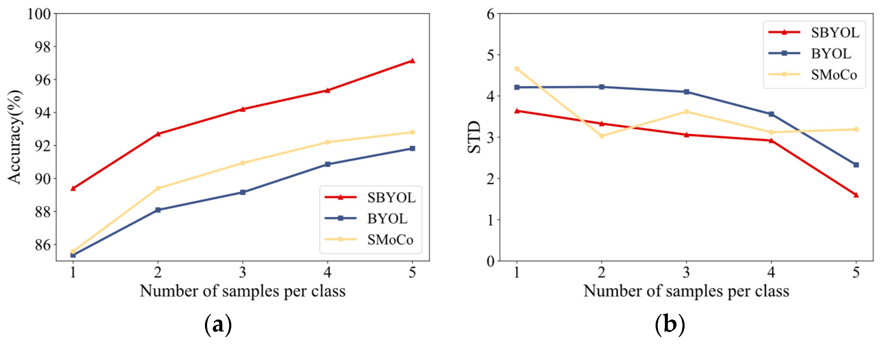
This paper further explores the performance of SBYOL in the case of extremely limited target training samples and uses the other two best-performing methods, BYOL and SMoCo, as a comparison. A total of five sets of experiments are conducted with training data sizes between 1 and 5 for each class, and the results are shown in

Table 4. Comparison results on DPS gear dataset under different volumes of training data.

Methods	Number of Samples per Class
	1	2	3	4	5
SBYOL	89.40 ± 3.64	92.70 ± 3.33	94.20 ± 3.06	95.34 ± 2.92	97.14 ± 1.60
BYOL	85.36 ± 4.21	88.09 ± 4.22	89.16 ± 4.10	90.86 ± 3.56	91.82 ± 2.33
SMoCo	85.58 ± 4.66	89.40 ± 3.03	90.94 ± 3.62	92.20 ± 3.12	92.80 ± 3.19

and Figure 12. In all cases, SBYOL achieved the best results, even with only two samples per class to achieve the best performance of other methods with five samples per class. In the extreme case of one sample per class, the accuracy decreases more due to the deviation from the classification plane, but even so, the best performance is achieved. As can be seen in Figure 12b, the stability of each method increases as the number of data increases, while SBYOL achieves the smallest STD in almost all cases. The results show that SBYOL has strong diagnostic performance and robustness against limited data conditions.

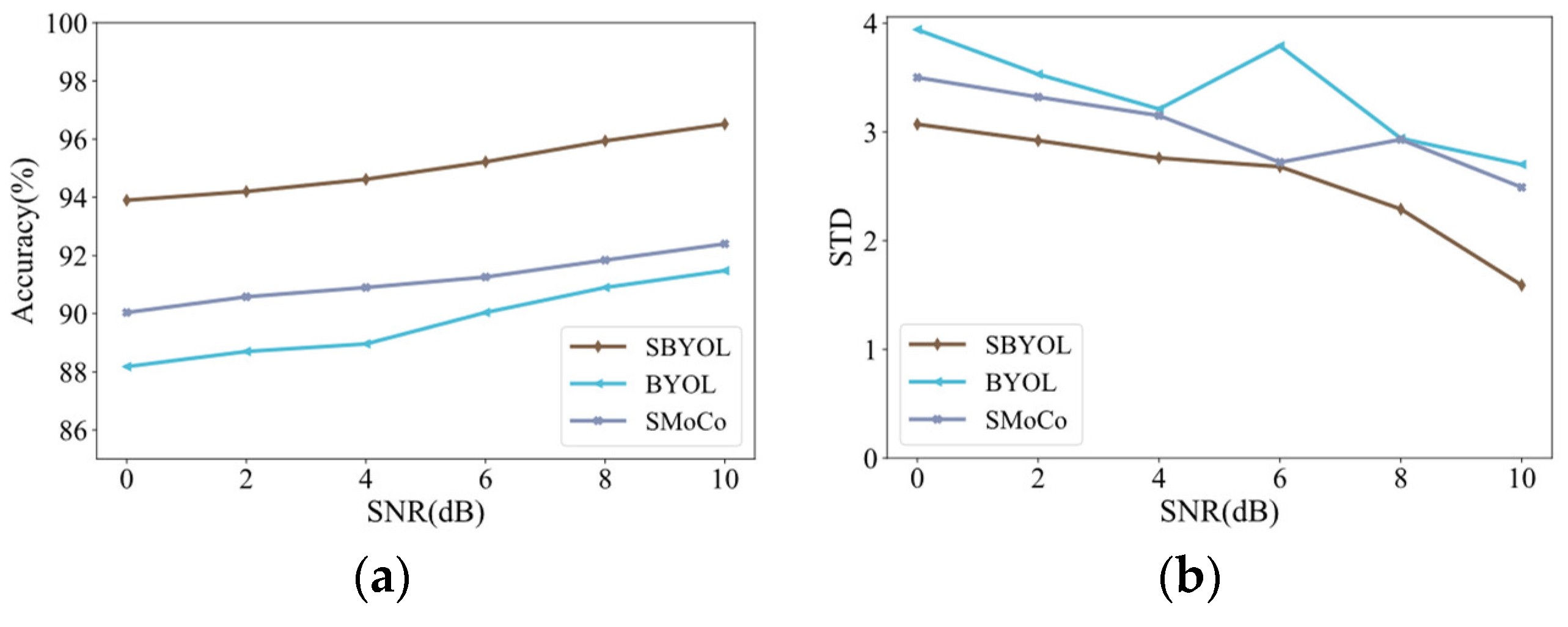
In addition, the noise interference immunity of SBYOL is further validated to demonstrate its robustness and effectiveness under different signal-to-noise ratio (SNR) conditions. The two best-performing methods BYOL and SMoCo are also selected for comparison. A total of six sets of experiments with an SNR from 0 to 10 are conducted for each method using the full training set, i.e., five samples per class, and the results are shown in

Table 5. Comparison results on DPS gear dataset under different SNRs.

Methods	SNR
	0 dB	2 dB	4 dB	6 dB	8 dB	10 dB
SBYOL	93.90 ± 3.07	94.20 ± 2.92	94.62 ± 2.76	95.22 ± 2.68	95.94 ± 2.29	96.52 ± 1.59
BYOL	88.18 ± 3.94	88.70 ± 3.53	88.96 ± 3.21	90.04 ± 3.79	90.90 ± 2.94	91.48 ± 2.70
SMoCo	90.04 ± 3.50	90.58 ± 3.32	90.90 ± 3.15	91.26 ± 2.72	91.84 ± 2.93	92.40 ± 2.49

and Figure 13. Compared with the two methods, SBYOL achieves the best results; even in the case of strong noise at 0 dB, it can achieve approximately 94% accuracy, proving its robustness to noise. In addition, as shown in Figure 13b, the overall standard deviation of SBYOL decreases as the noise diminishes, and is lower than the other two methods, which proves that SBYOL has good robustness to noise.

4.3. Verification on the Public Planetary Gearbox Dataset

To verify that the SBYOL pre-trained on parallel gearboxes can well solve the fault diagnosis of planetary gearboxes, the public SEU dataset is selected for further validation in this paper. The SEU dataset [34] provided by Southeast University was obtained on the drivetrain dynamic simulator (DDS), which contains two operating conditions with the rotating speed system load set to 20 Hz—0 V and 30 Hz—2 V, respectively. The test rig is shown in Figure 14. In each file, there are eight rows of vibration signals; in this paper, we use the second row of vibration signals, which means the x-axis vibration signal, and the length of each sample is still 4096. In addition, only 5 samples per class are used in the training set, and 50 samples per class are used in the testing set, and the specific information of the SEU dataset is shown in

Table 6. Labeled SEU gear dataset.

Fault Mode	Rotating Speed System Load	Training Samples	Testing Samples	Label
Health Gear	20 Hz—0 V	5	50	0
Health Gear	30 Hz—2 V	5	50	1
Chipped Tooth	20 Hz—0 V	5	50	2
Chipped Tooth	30 Hz—2 V	5	50	3
Missing Tooth	20 Hz—0 V	5	50	4
Missing Tooth	30 Hz—2 V	5	50	5
Root Fault	20 Hz—0 V	5	50	6
Root Fault	30 Hz—2 V	5	50	7
Surface Fault	20 Hz—0 V	5	50	8
Surface Fault	30 Hz—2 V	5	50	9

.

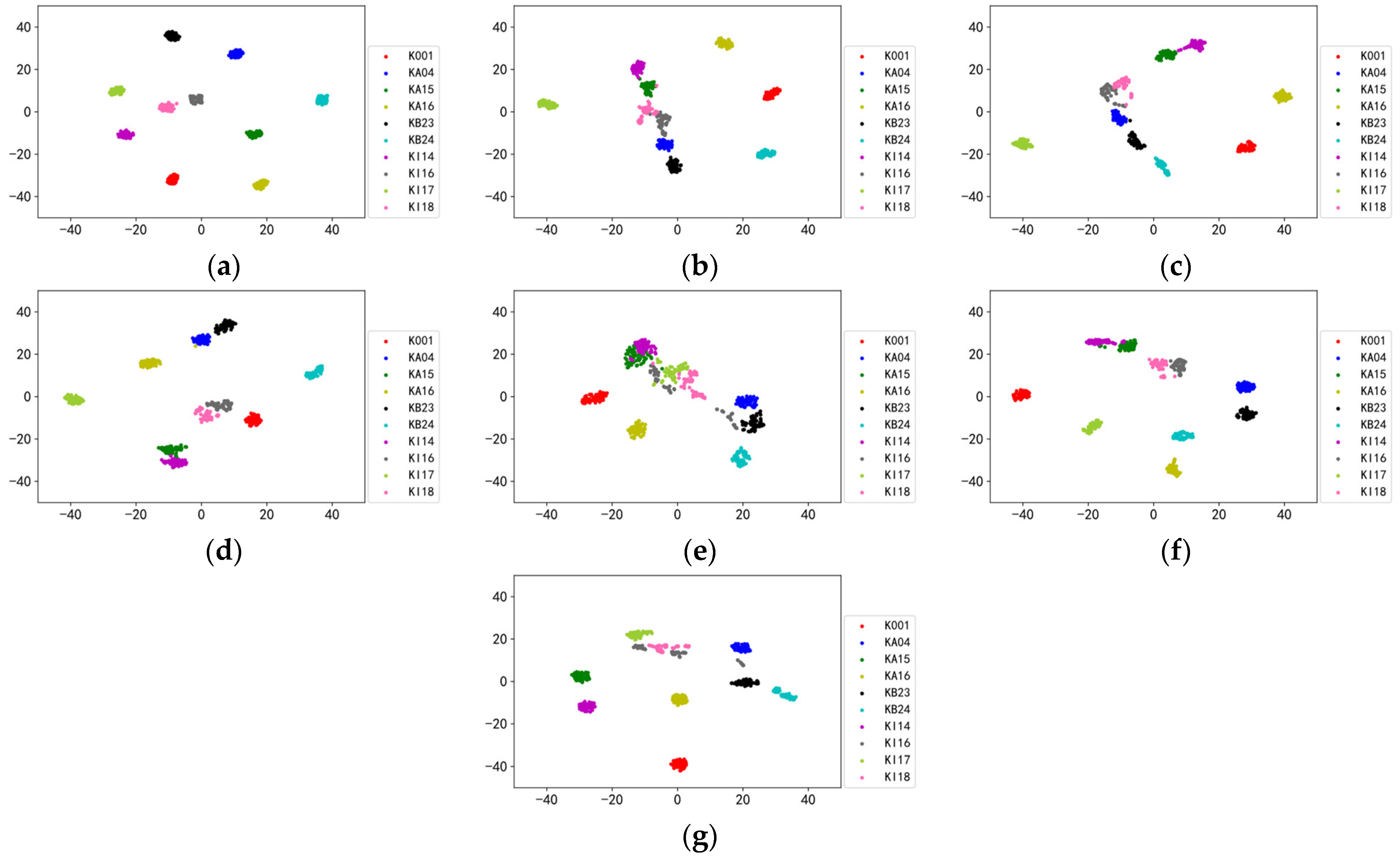
Similarly, feature extraction was performed on the SEU testing set using the feature extractors obtained by pre-training on the UoC dataset with fixed weights and visualized using T-SNE, and the results are shown in Figure 15. SBYOL can achieve excellent results in terms of extracted features without using any target diagnostic object for training, which is far better than other methods. SMoCo also achieves relatively good feature extraction results, but compared with SBYOL, the same category such as labels 5, 6, 7, 8, and 9 are not aggregated enough, and the two categories of labels 7 and 9 are too close to each other and are more prone to errors when there are limited training data.

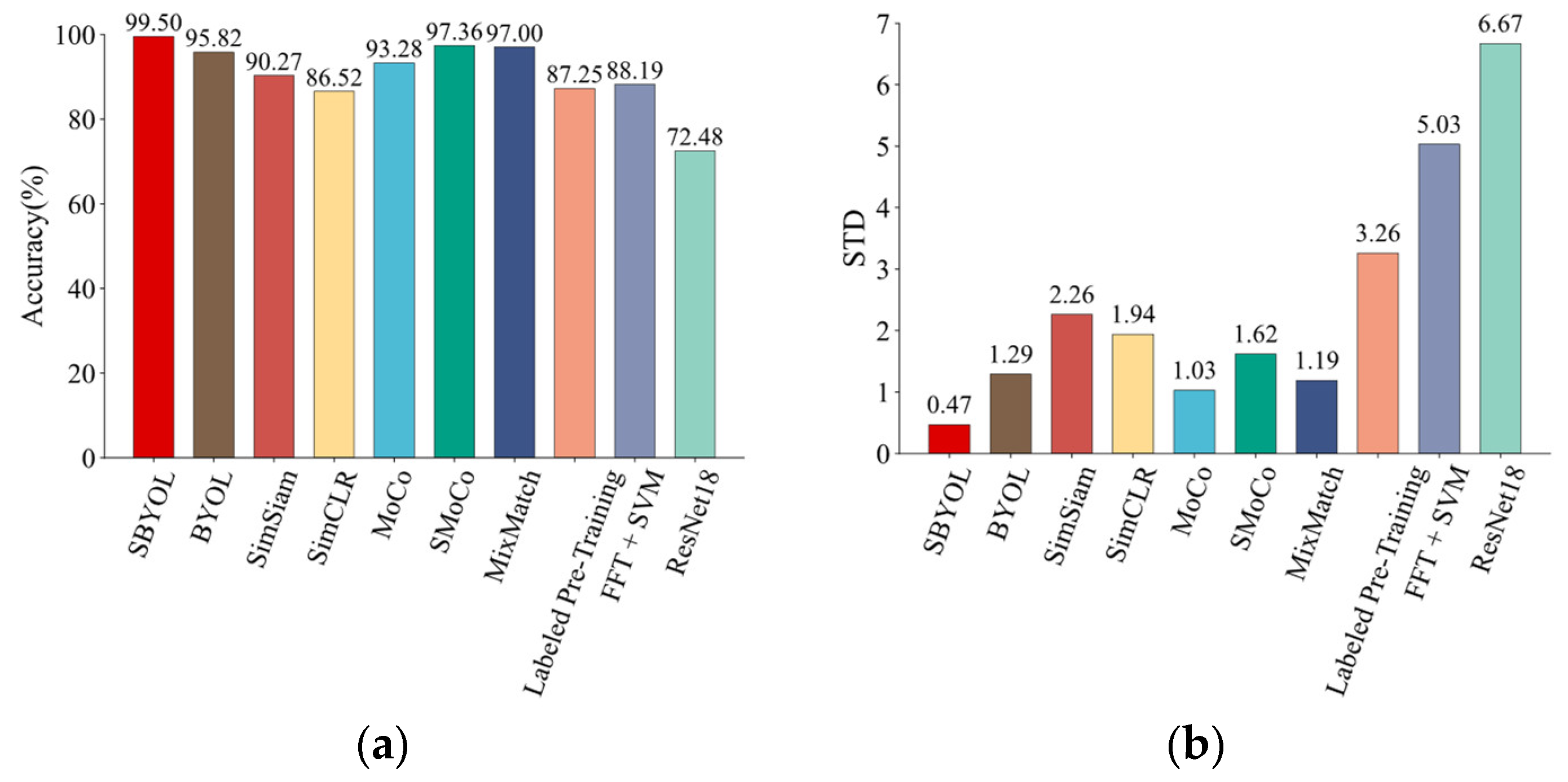
The same methods were used for fault diagnosis on the SEU dataset, and the results are shown in

Table 7. Comparison results on SEU gear dataset.

Method	Accuracy (%)	Time (s)
SBYOL	99.50 ± 0.47	2.35
BYOL	95.82 ± 1.29	2.25
SimSiam	90.27 ± 2.26	2.61
SimCLR	86.52 ± 1.94	2.55
MoCo	93.28 ± 1.03	2.56
SMoCo	97.36 ± 1.62	2.56
MixMatch	97.00 ± 1.19	1182.17
Labeled Pre-Training	87.25 ± 3.26	30.56
FFT + SVM	88.19 ± 5.03	0.11
ResNet18	72.48 ± 6.67	28.86

and Figure 16. The SBYOL method achieves the best diagnostic results in the face of a different device of the planetary gearbox, reaching an accuracy of 99.50%, which greatly exceeds other methods, and the STD of SBYOL is also only 0.47 because of its excellent feature extraction. Although SMoCo and MixMatch also achieve good diagnostic accuracy, they are still far inferior to SBYOL. In addition, since MixMatch needs to be retrained for each new diagnostic task, it is much slower than our method to apply it to the target diagnostic task.

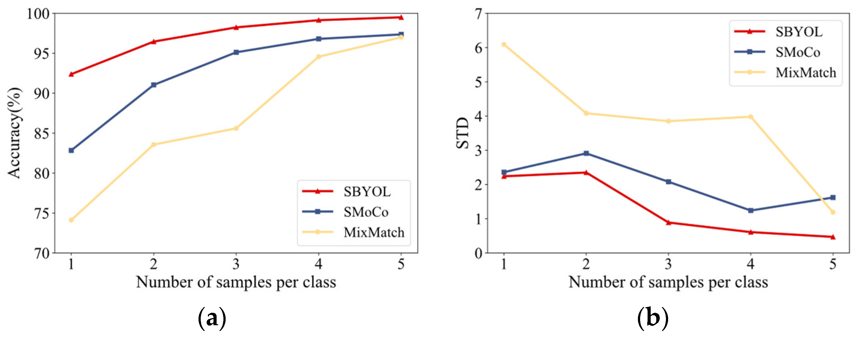
This paper also further explores the performance of SBYOL in the case of extremely limited training samples and selects the two best-performing methods, SMoCo and MixMatch, for comparison, and the results are shown in

Table 8. Comparison results on SEU gear dataset under different volumes of training data.

Methods	Number of Samples per Class
	1	2	3	4	5
SBYOL	92.38 ± 2.24	96.46 ± 2.35	98.24 ± 0.89	99.14 ± 0.61	99.50 ± 0.47
SMoCo	82.84 ± 2.36	91.04 ± 2.91	95.12 ± 2.08	96.80 ±1.24	97.36 ± 1.62
MixMatch	74.12 ± 6.09	83.57 ± 4.08	85.60 ± 3.85	94.57 ± 3.98	97.00 ± 1.19

and Figure 17. The best results are obtained for SBYOL with different training sample sizes, even with an accuracy of 98.24% for three samples per class. MixMatch’s performance is greatly degraded under extremely limited labeled datasets due to the lack of our unique data augmentation method. As can be seen in Figure 17b, the stability of each method increases as the number of data increases, while SBYOL achieves the smallest STD in all cases.

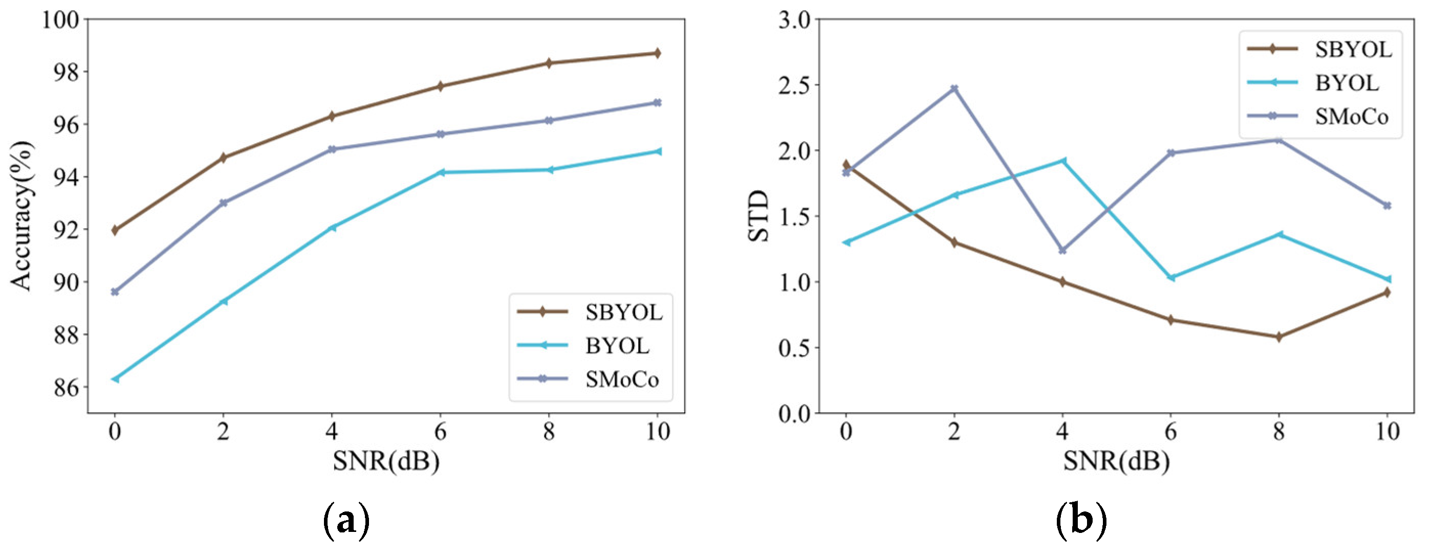
In addition, this paper further verifies the ability of SBYOL to resist noise interference. Since MixMatch does not have the unique data augmentation possessed by the self-supervised learning methods, its noise immunity is poor; two methods with good performance and stability, BYOL and SMoCo, are selected for comparison, and the results are shown in

Table 9. Comparison results on SEU gear dataset under different SNRs.

Methods	SNR
	0 dB	2 dB	4 dB	6 dB	8 dB	10 dB
SBYOL	91.96 ± 1.89	94.72 ± 1.30	96.30 ± 1.00	97.44 ± 0.71	98.32 ± 0.58	98.70 ± 0.92
BYOL	86.30 ± 1.30	89.26 ± 1.66	92.06 ± 1.92	94.16 ± 1.03	94.26 ± 1.36	94.96 ± 1.02
SMoCo	89.62 ± 1.83	93.00 ± 2.47	95.04 ± 1.24	95.62 ± 1.98	96.14 ± 2.08	96.82 ± 1.58

and Figure 18. Compared to these two methods, SBYOL achieves the best results, even at 4 dB, to reach the performance of the best-performing SMoCo at 10 dB, and its volatility is also the best in most cases. Excessive noise has a greater impact on diagnostic accuracy, but even so, it can achieve an accuracy of about 92% in the case of strong noise at 0 dB.

4.4. Verification on the Bearing Dataset

From the above experiments, the feature extractor obtained by SBYOL pre-training on the parallel gearbox well solves the fault diagnosis problem of planetary gearboxes. Therefore, to further validate that the pre-trained SBYOL learns a universal feature extractor, this section uses the PU bearing data and the PUT aero-engine high-speed bearing data as target diagnostic objects, respectively. The bearing data used have the characteristics of completely different types of equipment from the pre-training gear data.

The bearing dataset of Paderborn University (PU) was presented by Christian Lessmeier et al. [35] in 2016, and the experimental test rig is shown in Figure 19. In this dataset, there are multiple bearings divided into three main groups: 6 healthy bearings, 12 artificially damaged bearings, and 14 bearings with natural operation generating faults. The vibration signals were obtained at a sampling rate of 64 kHz and included four working conditions. It is a very difficult dataset in common datasets, which can reflect the difficulty of real fault diagnosis [37]. Ten types of real damaged bearings in the PU bearing dataset were selected as the target diagnostic dataset to better represent the actual problem, including one type of healthy bearings and two types of mixed faulty bearings. The operating condition is N15_M07_F04; specifically, the rotating speed is 1500 rpm, the loading torque is 0.7 NM, and the radial force is 400 N. The specific information is shown in

Table 10. Labeled PU bearing dataset.

Bearing Code	Damaged Element	Fault Mode	Damage Form	Arrangement	Damaged Extent
K001	Health state	/	/	/	/
KA04	Outer ring	Fatigue: pitting	Single damage	No repetition	Level 1
KA15	Outer ring	Plastic deform: Indentations	Single damage	No repetition	Level 1
KA16	Outer ring	Fatigue: pitting	Repetitive damage	Random	Level 2
KB23	Outer ring and inner ring	Fatigue: pitting	Multiple damage	Random	Level 2
KB24	Outer ring and inner ring	Fatigue: pitting	Multiple damage	No repetition	Level 3
KI14	Outer ring	Fatigue: pitting	Multiple damage	No repetition	Level 1
KI16	Outer ring	Fatigue: pitting	Single damage	No repetition	Level 3
KI17	Inner ring	Fatigue: pitting	Repetitive damage	Random	Level 1
KI18	Inner ring	Fatigue: pitting	Single damage	No repetition	Level 2

. To reflect the limited data problem faced in the actual diagnosis task, 5 samples are used for each class in the training set, and 50 samples are used for each class in the testing set.

Similarly, the pre-trained feature extractors are used to extract features from the PU bearing testing set with fixed weights and visualize them using T-SNE, and the results are shown in Figure 20. The SBYOL proposed in this paper achieves amazing feature extraction results for completely different types of bearing devices without using any data of the target diagnostic object for training, which greatly surpasses other methods.

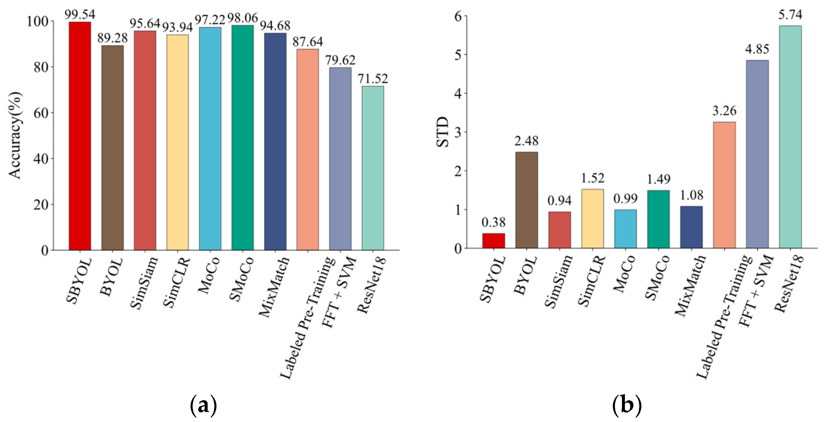
Next, fault diagnosis was performed on the PU dataset, and the results are shown in

Table 11. Comparison results on PU bearing dataset.

Method	Accuracy (%)	Time (s)
SBYOL	99.54 ± 0.38	2.38
BYOL	89.28 ± 2.48	2.39
SimSiam	95.64 ± 0.94	2.37
SimCLR	93.94 ± 1.52	2.35
MoCo	97.22 ± 0.99	2.37
SMoCo	98.06 ± 1.49	2.39
MixMatch	94.68 ± 1.08	1186.80
Labeled Pre-Training	87.64 ± 3.26	31.35
FFT + SVM	79.62 ± 4.85	0.10
ResNet18	71.52 ± 5.74	29.04

and Figure 21. When faced with a diagnostic problem for a completely different type of product, SBYOL achieves a diagnostic accuracy of 99.54%, which greatly exceeds other methods. SBYOL is approximately 12 times faster than Labeled Pre-Training and ResNet18, which require training neural networks, and approximately 500 times faster than MixMatch, which uses both a pre-training dataset and a target diagnostic dataset, when applied to diagnostic tasks. While Labeled Pre-Training can still improve accuracy, it is far less effective than SBYOL when faced with a diagnostic problem on a completely different device and without sufficient data for fine-tuning. In addition, since SBYOL achieves very good feature extraction without further training, its std is small, as shown in Figure 21b, proving its excellent stability even in the face of different types of bearing devices.

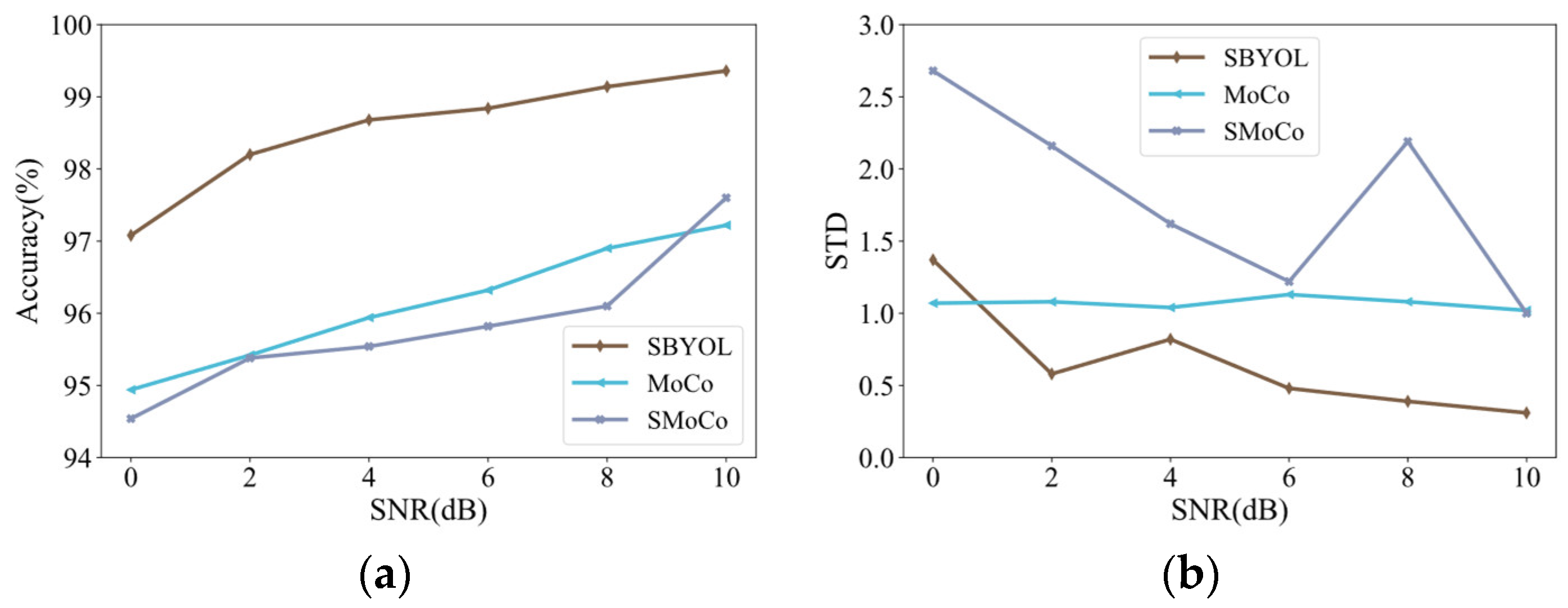
In this paper, the robustness of SBYOL is likewise verified for extremely limited data volumes and under different noises, and two other best-performing methods, MoCo and SMoCo, are selected for comparison; the results are shown in

Table 12. Comparison results on PU bearing dataset under different volumes of training data.

Methods	Number of Samples per Class
	1	2	3	4	5
SBYOL	94.52 ± 2.24	97.66 ± 1.21	98.50 ± 0.90	99.14 ± 0.91	99.54 ± 0.38
SMoCo	85.64 ± 4.01	92.92 ± 2.59	95.28 ± 1.76	96.56 ± 1.23	97.22 ± 0.99
MixMatch	81.48 ± 4.17	89.16 ± 3.98	95.32 ± 1.60	96.52 ± 2.12	98.06 ± 1.49

and

Table 13. Comparison results on PU bearing dataset under different SNRs.

Methods	SNR
	0 dB	2 dB	4 dB	6 dB	8 dB	10 dB
SBYOL	97.08 ± 1.37	98.20 ± 0.58	98.68 ± 0.82	98.84 ± 0.48	99.14 ± 0.39	99.36 ± 0.31
BYOL	94.94 ± 1.07	95.42 ± 1.08	95.94 ± 1.04	96.32 ± 1.13	96.90 ± 1.08	97.22 ± 1.02
SMoCo	94.54 ± 2.68	95.38 ± 2.16	95.54 ± 1.62	95.82 ± 1.22	96.10 ± 2.19	97.60 ± 1.00

and Figure 22 and Figure 23. SBYOL can achieve very high diagnostic accuracy even when facing the diagnostic problem of a completely different type of product such as a bearing, and it can achieve excellent accuracy in the case of extremely limited data and strong noise, greatly exceeding other methods. SBYOL can achieve a diagnostic accuracy of 94.52% with just one sample per class, and with only three samples per class, it can outperform other methods with five training samples per class. Although SBYOL can achieve good performance with one sample per class, it is prone to deviation from the classification plane in this case, and only two to three samples per class are needed to greatly improve the diagnostic accuracy of SBYOL. In addition, at 0 dB of strong noise, SBYOL even achieves the performance of other best-performing methods at 10 dB, greatly exceeding the performance of other methods. As shown in Figure 22b and Figure 23b, the overall stability of all methods continues to improve as the difficulty of diagnosis decreases, i.e., more training data and less noise.

Since SBYOL can achieve extremely high accuracy in the case of strong noise even in the face of completely different types of bearing devices, we further explored the cases of 0 dB, 4 dB, and 8 dB noise, whose corresponding feature extraction results are shown in Figure 24. With the enhancement of noise, the distance between categories keeps decreasing, and there is a gradual overlap between category KI16 and category KI18, so its diagnostic performance keeps decreasing. However, even with the strong noise of 0 dB, the categories are still well distinguished from each other, and the samples of the same category are aggregated, so it can achieve excellent and stable diagnostic accuracy.

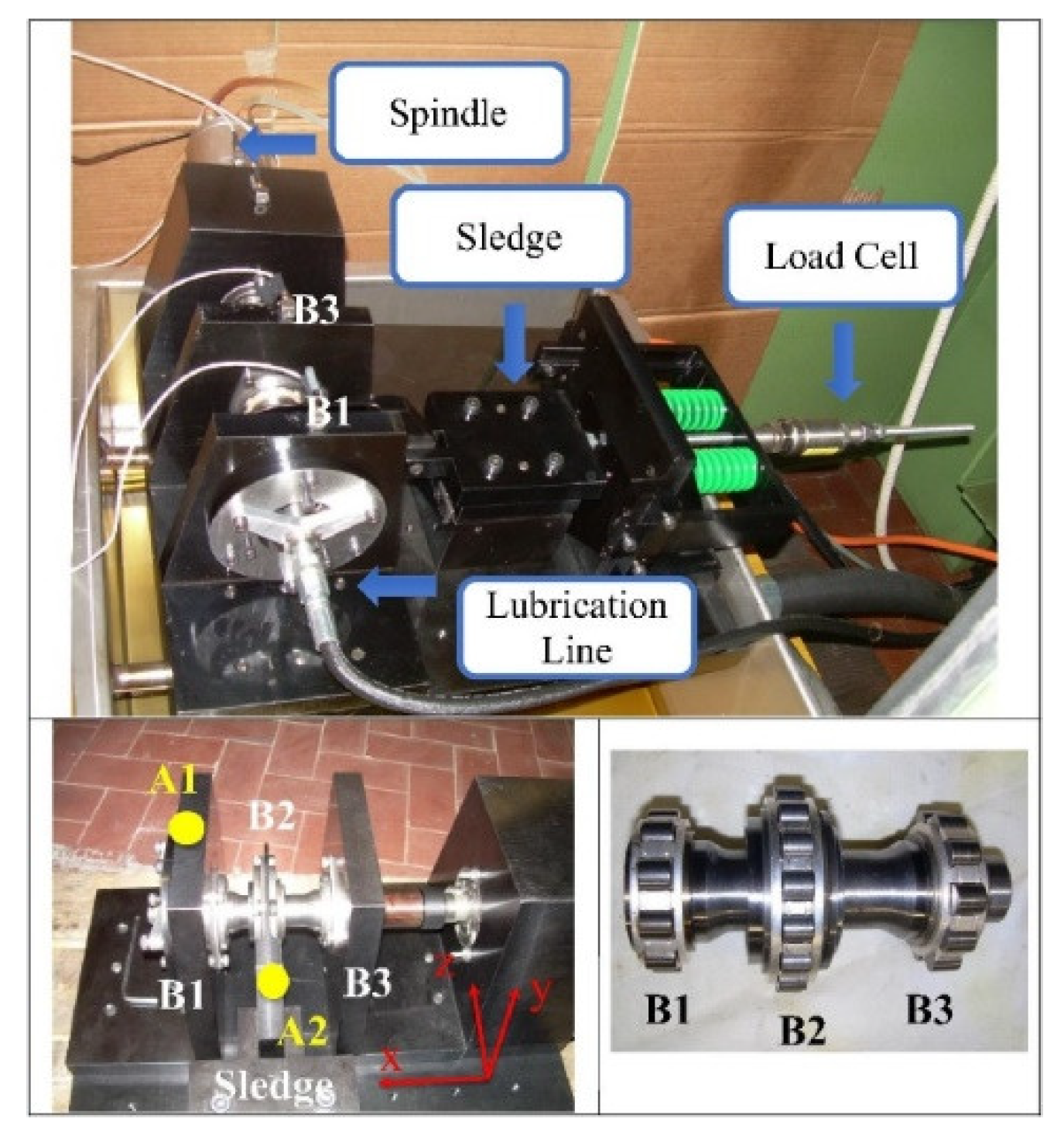
To verify the effectiveness of SBYOL more fully for completely different types of equipment, this paper uses the aero-engine high-speed bearing dataset from the Department of Mechanical and Aeronautical Engineering of the Polytechnic University of Turin (PUT), whose test rig is shown in Figure 25. For this dataset, we used the vibration acceleration data of aero-engine bearings at different speeds and different damage levels, with a sample length of 4096, and used the y-direction channel data at A1. To reflect the extremely limited data situation in the actual diagnosis process, only 3 samples per class were used in the training set, and 50 samples per class were used in the testing set. The specific dataset information is shown in

Table 14. Labeled PUT aero-engine bearing dataset.

Damaged Element	Diameter (μm)	Rotation Speed (r/min)	Load (N)	Training Samples	Testing Samples	Label
Healthy	/	24,000	1400	3	50	0
Inner ring	450	24,000	1400	3	50	1
Inner ring	250	24,000	1400	3	50	2
Inner ring	150	24,000	1400	3	50	3
Roller	450	24,000	1400	3	50	4
Roller	250	24,000	1400	3	50	5
Roller	150	24,000	1400	3	50	6
Inner ring	450	18,000	1400	3	50	7
Inner ring	250	18,000	1400	3	50	8
Inner ring	150	18,000	1400	3	50	9
Roller	450	18,000	1400	3	50	10
Roller	250	18,000	1400	3	50	11
Roller	150	18,000	1400	3	50	12

.

The pre-trained feature extractors are used to extract features from the PUT aero-engine high-speed bearing testing set and are visualized using T-SNE, and the results are shown in Figure 26. The SBYOL method proposed in this paper can achieve such extremely high feature extraction results for the aero-engine high-speed bearing data without using any data of the target diagnostic object for training, which greatly surpasses other methods with large segmentation intervals between categories and the aggregation of data within classes. SMoCo has also achieved good performance, but it is less aggregated than SBYOL for the category labeled 9, and its two categories labeled 7 and 9 are too close together.

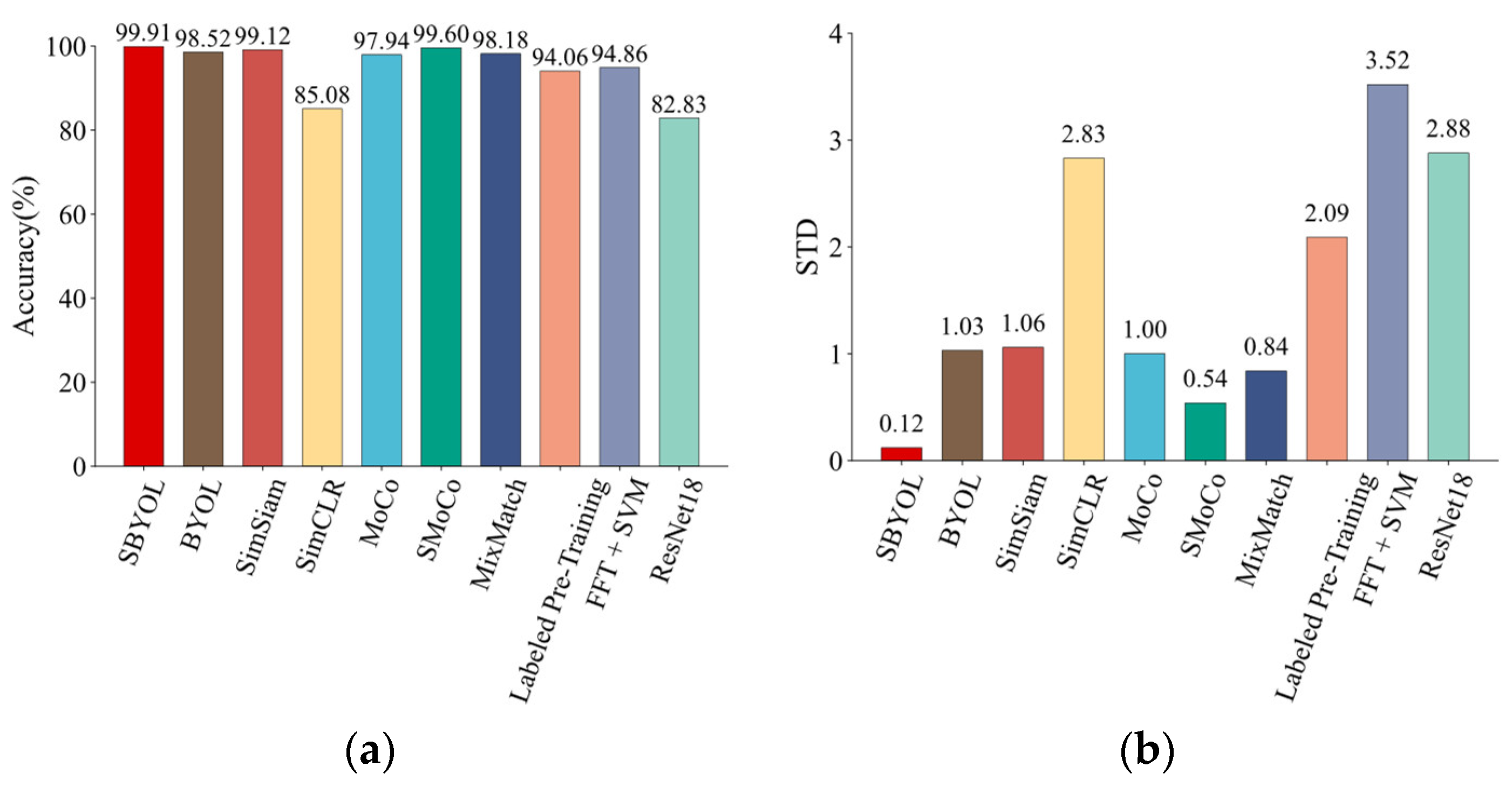
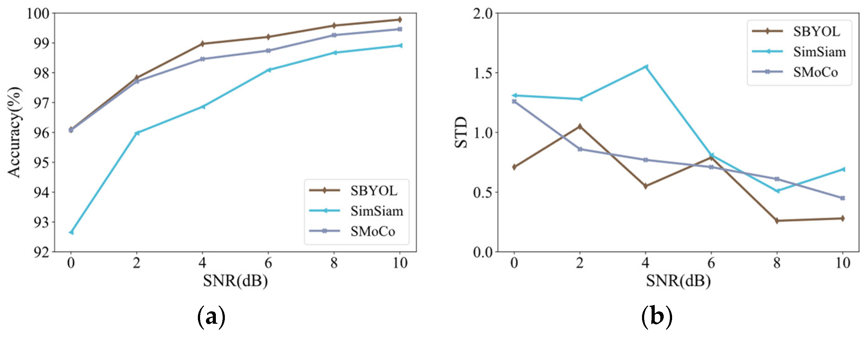
Similarly, the fault diagnosis is performed on the PUT aero-engine bearing dataset, and the results are shown in Table 15 and Figure 27. The robustness of SBYOL to the size of the training data and different levels of noise is further validated and compared with the two best-performing methods, and the results are shown in Table 16 and Table 17 and Figure 28 and Figure 29. SBYOL achieves the highest diagnostic accuracy and the smallest STD compared to other methods, even requiring only two samples per class to exceed the performance of SMoCo, which is the best performance among other methods. SBYOL also achieves the best performance in terms of noise immunity, with a diagnostic accuracy of 99.20% at 6 dB, which is comparable to the performance of SimSiam and SMoCo at 10 dB, proving that SBYOL is still robust to noise in the face of completely different devices. In addition, the STD of each method also shows a decreasing trend with the increase in data volume and the decrease in noise.

Table 15. Comparison results on PUT aero-engine bearing dataset.

Method	Accuracy (%)	Time (s)
SBYOL	99.91 ± 0.12	2.59
BYOL	98.52 ± 1.03	2.59
SimSiam	99.12 ± 1.06	2.56
SimCLR	85.08 ± 2.83	2.63
MoCo	97.94 ± 1.00	2.62
SMoCo	99.60 ± 0.54	2.60
MixMatch	98.18 ± 0.84	794.63
Labeled Pre-Training	94.06 ± 2.09	34.12
FFT + SVM	94.86 ± 3.52	0.11
ResNet18	82.83 ± 2.88	30.18

Table 15. Comparison results on PUT aero-engine bearing dataset.

Method	Accuracy (%)	Time (s)
SBYOL	99.91 ± 0.12	2.59
BYOL	98.52 ± 1.03	2.59
SimSiam	99.12 ± 1.06	2.56
SimCLR	85.08 ± 2.83	2.63
MoCo	97.94 ± 1.00	2.62
SMoCo	99.60 ± 0.54	2.60
MixMatch	98.18 ± 0.84	794.63
Labeled Pre-Training	94.06 ± 2.09	34.12
FFT + SVM	94.86 ± 3.52	0.11
ResNet18	82.83 ± 2.88	30.18

Figure 27. Comparison results on PUT aero-engine bearing dataset. (a) Accuracy; (b) standard deviation.

Figure 27. Comparison results on PUT aero-engine bearing dataset. (a) Accuracy; (b) standard deviation.

Table 16. Comparison results on PUT aero-engine bearing dataset under different volumes of training data.

Methods	Number of Samples per Class
	1	2	3
SBYOL	98.86 ± 0.21	99.82 ± 0.15	99.91 ± 0.12
SimSiam	95.82 ± 2.48	98.37 ± 1.35	99.12 ± 1.06
SMoCo	97.28 ± 1.88	98.85 ±1.23	99.60 ± 0.54

Table 16. Comparison results on PUT aero-engine bearing dataset under different volumes of training data.

Methods	Number of Samples per Class
	1	2	3
SBYOL	98.86 ± 0.21	99.82 ± 0.15	99.91 ± 0.12
SimSiam	95.82 ± 2.48	98.37 ± 1.35	99.12 ± 1.06
SMoCo	97.28 ± 1.88	98.85 ±1.23	99.60 ± 0.54

Figure 28. Comparison results on PUT aero-engine bearing dataset under different volumes of training data. (a) Accuracy; (b) standard deviation.

Figure 28. Comparison results on PUT aero-engine bearing dataset under different volumes of training data. (a) Accuracy; (b) standard deviation.

Table 17. Comparison results on PUT aero-engine bearing dataset under different SNRs.

Methods	SNR
	0 dB	2 dB	4 dB	6 dB	8 dB	10 dB
SBYOL	96.09 ± 0.71	97.83 ± 1.05	98.97 ± 0.55	99.20 ± 0.79	99.58 ± 0.26	99.78 ± 0.28
SimSiam	92.65 ± 1.31	95.98 ± 1.28	96.86 ± 1.55	98.09 ± 0.81	98.67 ± 0.51	98.91 ± 0.69
SMoCo	96.08 ± 1.26	97.71 ± 0.86	98.46 ± 0.77	98.74 ± 0.71	99.26 ± 0.61	99.46 ± 0.45

Table 17. Comparison results on PUT aero-engine bearing dataset under different SNRs.

Methods	SNR
	0 dB	2 dB	4 dB	6 dB	8 dB	10 dB
SBYOL	96.09 ± 0.71	97.83 ± 1.05	98.97 ± 0.55	99.20 ± 0.79	99.58 ± 0.26	99.78 ± 0.28
SimSiam	92.65 ± 1.31	95.98 ± 1.28	96.86 ± 1.55	98.09 ± 0.81	98.67 ± 0.51	98.91 ± 0.69
SMoCo	96.08 ± 1.26	97.71 ± 0.86	98.46 ± 0.77	98.74 ± 0.71	99.26 ± 0.61	99.46 ± 0.45

Figure 29. Comparison results on PUT aero-engine bearing dataset under different SNRs. (a) Accuracy; (b) standard deviation.

Figure 29. Comparison results on PUT aero-engine bearing dataset under different SNRs. (a) Accuracy; (b) standard deviation.

4.5. Robustness to Sampling Time and Data Size of the Pre-Training Dataset

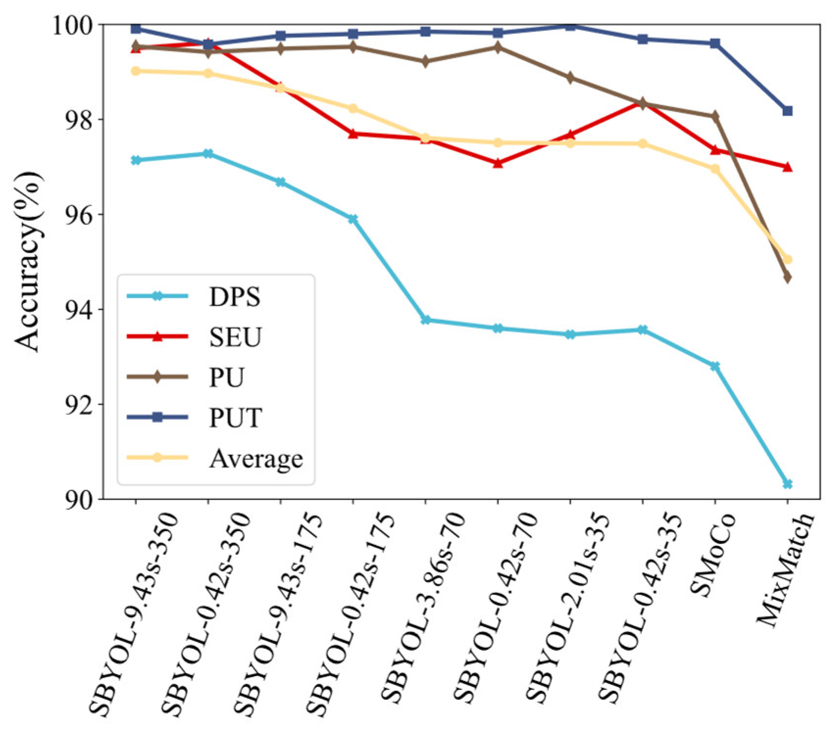
To further explore the requirements of SBYOL for pre-training datasets, in addition to the pre-training dataset size, the sampling time is also an influencing factor due to the unique data augmentation method TFST used by SBYOL. Therefore, this section further explores the robustness of SBYOL to the sampling time and data size of the pre-training dataset. Eight sets of experiments are conducted in this paper including SBYOL-9.43s-350, SBYOL-0.42s-350, SBYOL-9.43s-175, SBYOL-0.42s-175, SBYOL-3.86s-70, SBYOL-0.42s-70, SBYOL-2.01s-35, and SBYOL-0.42s-35. Taking SBYOL-9.43s-350 as an example, 9.43s represents the single sampling time, and 350 represents the number of samples per class in the pre-training dataset. These eight sets of experiments are self-supervised learning on the corresponding UoC pre-training datasets, and the learned feature extractors are then transferred to the DPS dataset, SEU dataset, PU dataset, and PUT dataset, respectively, where the training sets in the DPS dataset, SEU dataset, and PU dataset are still five samples per class, and the training sets in the PUT dataset are three samples per class. In addition, we also used the best-performing SMoCo and MixMatch as a comparison, which used all unlabeled pre-training datasets, i.e., 350 samples per class, and the results are shown in

Table 18. Comparison results of different sampling times and pre-training dataset sizes.

Method	Intercepted Sample Size	Data Size	DPS	SEU	PU	PUT	Average
SBYOL-9.43s-350	175	350 × 9	97.14	99.50	99.54	99.91	99.02
SBYOL-0.42s-350	5	350 × 9	97.28	99.61	99.42	99.58	98.97
SBYOL-9.43s-175	175	175 × 9	96.68	98.69	99.49	99.76	98.66
SBYOL-0.42s-175	5	175 × 9	95.90	97.70	99.53	99.80	98.23
SBYOL-3.86s-70	70	70 × 9	93.78	97.59	99.22	99.85	97.61
SBYOL-0.42s-70	5	70 × 9	93.60	97.08	99.52	99.82	97.51
SBYOL-2.01s-35	35	35 × 9	93.47	97.68	98.88	99.97	97.50
SBYOL-0.42s-35	5	35 × 9	93.57	98.37	98.33	99.69	97.49
SMoCo	/	350 × 9	92.80	97.36	98.06	99.60	96.96
MixMatch	/	350 × 9	90.32	97.00	94.68	98.18	95.05

and Figure 30.

SBYOL still achieves good performance with a smaller sampling time and pre-training dataset size, and the average diagnostic accuracy of SBYOL-0.42s-175 even reaches 98.23% on the four datasets. In addition, SBYOL-0.42s-35 achieves an average diagnostic accuracy of 97.49%, surpassing SMoCo and MixMatch, the best performers among other methods, while only using 10% of the dataset size compared to SMoCo and MixMatch. From comparing SBYOL-9.43s-350 with SBYOL-0.42s-350, SBYOL-9.43s-175 with SBYOL-0.42s-175, SBYOL-3.86s-70 with SBYOL-0.42s-70, and SBYOL-2.01s-35 with SBYOL-0.42s-35, with the same amount of data, a longer sampling signal allows SBYOL to perform better on average over the four datasets. From the comparison of SBYOL-0.42s-350 with SBYOL-9.43s-175, SBYOL-0.42s-175 with SBYOL-3.86s-70, and SBYOL-0.42s-70 with SBYOL-2.01s-35, SBYOL can perform better with a larger amount of data even with shorter sampling time. The performance is closer in the case of 70 and 35 samples per class compared to the difference between 350, 175, and 70 samples per class, proving that it still requires a larger variation in data volume for a larger improvement in performance.

Therefore, from the above results, SBYOL is extremely robust to the pre-training dataset, longer sampling time and larger datasets can achieve better performance, and dataset size improves performance more than sampling time when there is a large difference in dataset size.

5. Conclusions

The problem of limited data and strong noise in the rotating machinery fault diagnosis tasks under real conditions seriously affects the performance of intelligent diagnosis methods. In this paper, we innovatively propose SBYOL for the automatic feature extraction of unlabeled rotating machinery vibration signals, which incorporates the novel data augmentation method TFST proposed in this paper to retain both time domain and frequency domain information of the signal at the same time. SBYOL first performs self-supervised learning on easily available unlabeled data and then uses the trained feature extractor for downstream diagnostic tasks under limited data. In this paper, a powerful and robust universal feature extractor was constructed by self-supervised pre-training on the unlabeled UoC parallel gearbox dataset and then applied to a private DPS planetary gearbox dataset under limited data, achieving an accuracy of 97.14%. It was further validated on the SEU planetary gearbox dataset and achieved an accuracy of 99.50%. To further demonstrate that SBYOL learned a universal feature extractor, two public bearing datasets, the PU and PUT bearing datasets, with completely different types of devices compared to the pre-training dataset, were used as target diagnostic objects, both achieving diagnostic accuracy of over 99.54%. Further experiments show that SBYOL also has excellent performance for the target diagnostic object under extremely limited data and strong noise and is robust to the unlabeled pre-training dataset with a shorter sampling time and smaller data size, demonstrating its great potential and superiority for rotating machinery fault diagnosis problems.

Although SBYOL achieved excellent results, there are still some works that deserve further exploration. In the self-supervised signal representation learning stage, SBYOL takes a relatively long time to learn a good representation of the signal, and future research can be conducted on how to improve the training efficiency, such as using mixed precision training. For the structure of the encoder, future work can also try to use a transformer network that currently performs well in various fields. Finally, although SBYOL showed promising results under steady-state operating conditions, there is a lack of exploration regarding fault diagnosis under varying operating conditions. Therefore, future research can further investigate and explore more data transformation methods that are suitable for handling varying operating conditions [41,42].

References

1. Khan, S.; Yairi, T. A review on the application of deep learning in system health management. Mech. Syst. Signal Process. 2018, 107, 241–265. [Google Scholar] [CrossRef]
2. Lei, Y.; Yang, B.; Jiang, X.; Jia, F.; Li, N.; Nandi, A.K. Applications of machine learning to machine fault diagnosis: A review and roadmap. Mech. Syst. Signal Process. 2020, 138, 106587. [Google Scholar] [CrossRef]
3. Chen, H.; Meng, W.; Li, Y.; Xiong, Q. An anti-noise fault diagnosis approach for rolling bearings based on multiscale CNN-LSTM and a deep residual learning model. Meas. Sci. Technol. 2023, 34, 045013. [Google Scholar] [CrossRef]
4. Mian, T.; Choudhary, A.; Fatima, S. Vibration and infrared thermography based multiple fault diagnosis of bearing using deep learning. Nondestruct. Test. Eval. 2023, 38, 275–296. [Google Scholar] [CrossRef]
5. Bai, R.; Xu, Q.; Meng, Z.; Cao, L.; Xing, K.; Fan, F. Rolling bearing fault diagnosis based on multi-channel convolution neural network and multi-scale clipping fusion data augmentation. Measurement 2021, 184, 109885. [Google Scholar] [CrossRef]
6. Feng, Y.; Chen, J.; Zhang, T.; He, S.; Xu, E.; Zhou, Z. Semi-supervised meta-learning networks with squeeze-and-excitation attention for few-shot fault diagnosis. ISA Trans. 2022, 120, 383–401. [Google Scholar] [CrossRef]
7. Wu, X.; Zhang, Y.; Cheng, C.; Peng, Z. A hybrid classification autoencoder for semi-supervised fault diagnosis in rotating machinery. Mech. Syst. Signal Process. 2021, 149, 107327. [Google Scholar] [CrossRef]
8. Zhao, X.; Jia, M.; Liu, Z. Semisupervised Deep Sparse Auto-Encoder with Local and Nonlocal Information for Intelligent Fault Diagnosis of Rotating Machinery. IEEE Trans. Instrum. Meas. 2021, 70, 1–13. [Google Scholar] [CrossRef]
9. Li, J.; Huang, R.; Li, W. Intelligent Fault Diagnosis for Bearing Dataset Using Adversarial Transfer Learning based on Stacked Auto-Encoder. Procedia Manuf. 2020, 49, 75–80. [Google Scholar] [CrossRef]
10. Han, T.; Liu, C.; Yang, W.; Jiang, D. Deep transfer network with joint distribution adaptation: A new intelligent fault diagnosis framework for industry application. ISA Trans. 2020, 97, 269–281. [Google Scholar] [CrossRef] [PubMed] [Green Version]
11. Zheng, H.; Wang, R.; Yang, Y.; Yin, J.; Li, Y.; Li, Y.; Xu, M. Cross-Domain Fault Diagnosis Using Knowledge Transfer Strategy: A Review. IEEE Access 2019, 7, 129260–129290. [Google Scholar] [CrossRef]
12. Jing, L.; Tian, Y. Self-Supervised Visual Feature Learning with Deep Neural Networks: A Survey. IEEE Trans. Pattern Anal. Mach. Intell. 2021, 43, 4037–4058. [Google Scholar] [CrossRef] [PubMed]
13. Zhang, R.; Isola, P.; Efros, A.A. Colorful Image Colorization. In Computer Vision–ECCV 2016; Leibe, B., Matas, J., Sebe, N., Welling, M., Eds.; Lecture Notes in Computer Science; Springer International Publishing: Cham, Switzerland, 2016; Volume 9907, pp. 649–666. [Google Scholar] [CrossRef] [Green Version]
14. Pathak, D.; Krähenbühl, P.; Donahue, J.; Darrell, T.; Efros, A.A. Context Encoders: Feature Learning by Inpainting. In Proceedings of the 2016 IEEE Conference on Computer Vision and Pattern Recognition (CVPR), Las Vegas, NV, USA, 27−30 June 2016; pp. 2536–2544. [Google Scholar] [CrossRef] [Green Version]
15. Noroozi, M.; Favaro, P. Unsupervised Learning of Visual Representations by Solving Jigsaw Puzzles. In Computer Vision–ECCV 2016; Leibe, B., Matas, J., Sebe, N., Welling, M., Eds.; Lecture Notes in Computer Science 9910; Springer International Publishing: Cham, Switzerland, 2016; pp. 69–84. [Google Scholar] [CrossRef] [Green Version]
16. Ledig, C.; Theis, L.; Huszár, F.; Caballero, J.; Cunningham, A.; Acosta, A.; Aitken, A.P.; Tejani, A.; Totz, J.; Wang, Z.; et al. Photo-Realistic Single Image Super-Resolution Using a Generative Adversarial Network. In Proceedings of the 2017 IEEE Conference on Computer Vision and Pattern Recognition (CVPR), Honolulu, HI, USA, 21–26 July 2017; pp. 105–114. [Google Scholar] [CrossRef] [Green Version]
17. Rani, V.; Nabi, S.T.; Kumar, M.; Mittal, A.; Kumar, K. Self-supervised Learning: A Succinct Review. Arch. Comput. Methods Eng. 2023, 30, 2761–2775. [Google Scholar] [CrossRef] [PubMed]
18. Grill, J.-B.; Strub, F.; Altché, F.; Tallec, C.; Richemond, P.H.; Buchatskaya, E.; Doersch, C.; Pires, B.A.; Guo, Z.D.; Azar, M.G.; et al. Bootstrap your own latent: A new approach to self-supervised Learning. arXiv 2020, arXiv:2006.07733. [Google Scholar]
19. Tian, Y.; Sun, C.; Poole, B.; Krishnan, D.; Schmid, C.; Isola, P. What Makes for Good Views for Contrastive Learning? In Advances in Neural Information Processing Systems; Curran Associates Inc.: Vancouver, BC, Canada, 2020; pp. 6827–6839. Available online: https://papers.nips.cc/paper/2020/hash/4c2e5eaae9152079b9e95845750bb9ab-Abstract.html (accessed on 19 April 2022).
20. Chen, T.; Kornblith, S.; Norouzi, M.; Hinton, G. A Simple Framework for Contrastive Learning of Visual Representations. In Proceedings of the 37th International Conference on Machine Learning, PMLR, November 2020, 1597–1607; Available online: https://proceedings.mlr.press/v119/chen20j.html (accessed on 18 April 2022).
21. Chen, T.; Kornblith, S.; Swersky, K.; Norouzi, M.; Hinton, G.E. Big Self-Supervised Models are Strong Semi-Supervised Learners. In Advances in Neural Information Processing Systems; Curran Associates, Inc.: Vancouver, BC, Canada, 2020; pp. 22243–22255. Available online: https://proceedings.neurips.cc/paper/2020/hash/fcbc95ccdd551da181207c0c1400c655-Abstract.html (accessed on 19 April 2022).
22. Wang, H.; Liu, Z.; Ge, Y.; Peng, D. Self-supervised signal representation learning for machinery fault diagnosis under limited annotation data. Knowl.-Based Syst. 2022, 239, 107978. [Google Scholar] [CrossRef]
23. Ding, Y.; Zhuang, J.; Ding, P.; Jia, M. Self-supervised pretraining via contrast learning for intelligent incipient fault detection of bearings. Reliab. Eng. Syst. Saf. 2022, 218, 108126. [Google Scholar] [CrossRef]
24. He, K.; Fan, H.; Wu, Y.; Xie, S.; Girshick, R. Momentum Contrast Unsupervised Vis. Represent. Learning. arxiv 2020, arXiv:1911.05722. [Google Scholar]
25. Wei, M.; Liu, Y.; Zhang, T.; Wang, Z.; Zhu, J. Fault Diagnosis of Rotating Machinery Based on Improved Self-Supervised Learning Method and Very Few Labeled Samples. Sensors 2021, 22, 192. [Google Scholar] [CrossRef]
26. Yan, Z.; Liu, H. SMoCo: A Powerful and Efficient Method Based on Self-Supervised Learning for Fault Diagnosis of Aero-Engine Bearing under Limited Data. Mathematics 2022, 10, 2796. [Google Scholar] [CrossRef]
27. Shul, Y.; Yi, W.; Choi, J.; Kang, D.-S.; Choi, J.-W. Noise-based self-supervised anomaly detection in washing machines using a deep neural network with operational information. Mech. Syst. Signal Process. 2023, 189, 110102. [Google Scholar] [CrossRef]
28. Nie, G.; Zhang, Z.; Shao, M.; Jiao, Z.; Li, Y.; Li, L. A Novel Study on a Generalized Model Based on Self-Supervised Learning and Sparse Filtering for Intelligent Bearing Fault Diagnosis. Sensors 2023, 23, 1858. [Google Scholar] [CrossRef]
29. Jaiswal, A.; Babu, A.R.; Zadeh, M.Z.; Banerjee, D.; Makedon, F. A Survey on Contrastive Self-Supervised Learning. Technologies 2020, 9, 2. [Google Scholar] [CrossRef]
30. He, K.; Zhang, X.; Ren, S.; Sun, J. Deep Residual Learning for Image Recognition. In Proceedings of the 2016 IEEE Conference on Computer Vision and Pattern Recognition (CVPR), Las Vegas, NV, USA, 27–30 June 2016; pp. 770–778. [Google Scholar] [CrossRef] [Green Version]
31. Ioffe, S.; Szegedy, C. Batch Normalization: Accelerating Deep Network Training by Reducing Internal Covariate Shift. arXiv 2015, arXiv:1502.03167. [Google Scholar]
32. Cao, P.; Zhang, S.; Tang, J. Gear Fault Data. figshare, April 11 2018. Available online: https://figshare.com/articles/dataset/Gear_Fault_Data/6127874/1 (accessed on 22 March 2022).
33. Cao, P.; Zhang, S.; Tang, J. Preprocessing-Free Gear Fault Diagnosis Using Small Datasets with Deep Convolutional Neural Network-Based Transfer Learning. IEEE Access 2018, 6, 26241–26253. [Google Scholar] [CrossRef]
34. Shao, S.; McAleer, S.; Yan, R.; Baldi, P. Highly Accurate Machine Fault Diagnosis Using Deep Transfer Learning. IEEE Trans. Ind. Inf. 2019, 15, 2446–2455. [Google Scholar] [CrossRef]
35. Lessmeier, C.; Kimotho, J.K.; Zimmer, D.; Sextro, W. Condition Monitoring of Bearing Damage in Electromechanical Drive Systems by Using Motor Current Signals of Electric Motors: A Benchmark Data Set for Data-Driven Classification. PHM Soc. Eur. Conf. 2016, 3, 1. [Google Scholar] [CrossRef]
36. Daga, A.P.; Fasana, A.; Marchesiello, S.; Garibaldi, L. The Politecnico di Torino rolling bearing test rig: Description and analysis of open access data. Mech. Syst. Signal Process. 2019, 120, 252–273. [Google Scholar] [CrossRef]
37. Zhao, Z.; Li, T.; Wu, J.; Sun, C.; Wang, S.; Yan, R.; Chen, X. Deep learning algorithms for rotating machinery intelligent diagnosis: An open source benchmark study. ISA Trans. 2020, 107, 224–255. [Google Scholar] [CrossRef]
38. Zhang, X.; He, C.; Lu, Y.; Chen, B.; Zhu, L.; Zhang, L. Fault diagnosis for small samples based on attention mechanism. Measurement 2022, 187, 110242. [Google Scholar] [CrossRef]
39. Chen, X.; He, K. Exploring Simple Siamese Representation Learning. arXiv 2020, arXiv:2011.10566. [Google Scholar]
40. Berthelot, D.; Carlini, N.; Goodfellow, I.; Papernot, N.; Oliver, A.; Raffel, C.A. MixMatch: A Holistic Approach to Semi-Supervised Learning. In Advances in Neural Information Processing Systems; Curran Associates Inc.: Vancouver, BC, Canada, 2019; Available online: https://proceedings.neurips.cc/paper/2019/hash/1cd138d0499a68f4bb72bee04bbec2d7-Abstract.html (accessed on 21 June 2022).
41. Luo, Z.; Tan, H.; Dong, X.; Zhu, G.; Li, J. A fault diagnosis method for rotating machinery with variable speed based on multi-feature fusion and improved ShuffleNet V2. Meas. Sci. Technol. 2023, 34, 035110. [Google Scholar] [CrossRef]
42. Zhang, K.; Wang, J.; Shi, H.; Zhang, X. A Variable Working Condition Rolling Bearing Fault Diagnosis Method Based on Improved Triplet Loss Algorithm. Int. J. Control Autom. Syst. 2023, 21, 1361–1372. [Google Scholar] [CrossRef]
Figure 1. Flow chart of fault diagnosis based on SBYOL.
Aerospace 10 00681 g001
Figure 2. Examples of six basic data augmentation methods: (a) Normalize; (b) AddGaussian; (c) Scale; (d) Stretch; (e) Crop; (f) Flip.
Aerospace 10 00681 g002
Figure 3. The framework of TFST.
Aerospace 10 00681 g003
Figure 4. The network structure of SBYOL with ResNet-18 encoder.
Aerospace 10 00681 g004
Figure 5. Test rig of UoC dataset [38].
Aerospace 10 00681 g005
Figure 6. Loss curve in the self-supervised signal representation learning stage.
Aerospace 10 00681 g006
Figure 7. The visualization of pre-trained feature extractors on unlabeled UoC gear dataset. (a) SBYOL; (b) Labeled Pre-Training; (c) SimSiam; (d) SimCLR; (e) BYOL; (f) MoCo; (g) SMoCo.
Aerospace 10 00681 g007
Figure 8. The DPS test rig. (a) Tset rig; (b) End cap vibration sensor; (c) Box vibration sensor.
Aerospace 10 00681 g008
Figure 9. Gears with four failure modes in the DPS test rig. (a) Wear; (b) broken tooth; (c) missing tooth; (d) root crack.
Aerospace 10 00681 g009
Figure 10. The visualization of pre-trained feature extractors on the DPS gear dataset. (a) SBYOL; (b) Labeled Pre-Training; (c) SimSiam; (d) SimCLR; (e) BYOL; (f) MoCo; (g) SMoCo.
Aerospace 10 00681 g010
Figure 11. Comparison results on DPS gear dataset. (a) Accuracy; (b) standard deviation.
Aerospace 10 00681 g011
Figure 12. Comparison results on DPS gear dataset under different volumes of training data. (a) Accuracy; (b) standard deviation.
Aerospace 10 00681 g012
Figure 13. Comparison results on DPS gear dataset under different SNRs. (a) Accuracy; (b) standard deviation.
Aerospace 10 00681 g013
Figure 14. Test rig of SEU dataset [34].
Aerospace 10 00681 g014
Figure 15. The visualization of pre-trained feature extractors on the SEU gear dataset. (a) SBYOL; (b) Labeled Pre-Training; (c) SimSiam; (d) SimCLR; (e) BYOL; (f) MoCo; (g) SMoCo.
Aerospace 10 00681 g015
Figure 16. Comparison results on SEU gear dataset. (a) Accuracy; (b) standard deviation.
Aerospace 10 00681 g016
Figure 17. Comparison results on SEU gear dataset under different volumes of training data. (a) Accuracy; (b) standard deviation.
Aerospace 10 00681 g017
Figure 18. Comparison results on SEU gear dataset under different SNRs. (a) Accuracy; (b) standard deviation.
Aerospace 10 00681 g018
Figure 19. Test rig of PU dataset. (a) Electric motor; (b) torque-measurement shaft; (c) rolling bearing test module; (d) flywheel; (e) load motor.
Aerospace 10 00681 g019
Figure 20. The visualization of pre-trained feature extractors on the PU bearing dataset. (a) SBYOL; (b) Labeled Pre-Training; (c) SimSiam; (d) SimCLR; (e) BYOL; (f) MoCo; (g) SMoCo.
Aerospace 10 00681 g020
Figure 21. Comparison results on PU bearing dataset. (a) Accuracy; (b) standard deviation.
Aerospace 10 00681 g021
Figure 22. Comparison results on PU bearing dataset under different volumes of training data. (a) Accuracy; (b) standard deviation.
Aerospace 10 00681 g022
Figure 23. Comparison results on PU bearing dataset under different SNRs. (a) Accuracy; (b) standard deviation.
Aerospace 10 00681 g023
Figure 24. Visualization of SBYOL on noisy PU bearing datasets. (a) 0 dB; (b) 4 dB; (c) 8 dB.
Aerospace 10 00681 g024
Figure 25. Test rig of the aero-engine bearing dataset from the Polytechnic University of Turin [36].
Aerospace 10 00681 g025
Figure 26. The visualization of pre-trained feature extractors on the PUT aero-engine bearing dataset. (a) SBYOL; (b) Labeled Pre-Training; (c) SimSiam; (d) SimCLR; (e) BYOL; (f) MoCo; (g) SMoCo.
Aerospace 10 00681 g026
Figure 30. Comparison results of different sampling times and pre-training dataset sizes.
Aerospace 10 00681 g030