Potential Propulsive and Aerodynamic Benefits of a New Aircraft Concept: A Low-Speed Experimental Study

Abstract

The aerodynamic design of a new aircraft concept was investigated through subsonic wind-tunnel testing using 1:28-scale powered models. The aircraft configuration integrates a box-wing layout with engines located at the rear part of the fuselage. Measurements involved a back-to-back comparison between two aircraft models: a podded version whose engines were assembled on pylons and a boundary-layer ingestion (BLI) version that provided several system-level benefits. The flowfield was investigated through the power balance method and a variety of pressure flowfield and inlet flow distortion metrics. The results proved that the BLI configuration enhances the propulsive efficiency by reducing both the electrical power coefficient and the kinetic energy waste due to lower jet velocities. Furthermore, there was a reduction of the total pressure recovery due to pressure gradients inside the duct, thereby causing high distortion. Overall, this research highlights the importance of wind-tunnel testing to bring any aerodynamic technology to a sufficient level of maturity and to enable future new aircraft concepts.

1. Introduction

Designing new aircraft concepts that aim to reduce climate change is a crucial aspect of the ongoing efforts to mitigate the environmental impact of aviation. The objective behind these designs is to develop aircraft that are more fuel efficient, emit fewer greenhouse gases, and minimize other detrimental effects on the environment. One area of focus is improving aerodynamic efficiency by incorporating features such as blended-wing bodies, non-planar wings, or unconventional wingtip designs that enhance lift-to-drag ratios. These improvements reduce the amount of fuel required to propel the aircraft, thus resulting in lower carbon dioxide (CO${}_2$) emissions [1]. Furthermore, advanced propulsion systems, such as hybrid-electric propulsion, boundary-layer Ingestion (BLI) engines, hydrogen fuel cells, and others, can reduce the reliance on conventional jet engines and fossil fuels [2,3]. Another consideration is the use of lightweight and sustainable materials in aircraft construction. Utilizing advanced composite materials or bio-based materials can reduce the weight of the aircraft, thereby leading to decreased fuel consumption and emissions [4].

Several concepts have been proposed over the past few years based on such technologies, thus encouraging the further exploration of unconventional aircraft for long-term sustainable flying. Some configurations include the blended-wing body (BWB), which merges the fuselage and wings into a single, smoothly blended structure. The BWB offers improved aerodynamic efficiency, increased passenger capacity, and potential fuel savings due to a reduced drag and an increased lift-to-drag ratio [5,6]. The box-wing concept is characterized by multiple wing sections that are interconnected to form a box-like structure. Box-wings offer potential advantages, such as an improved lift-to-drag ratio, increased stability, and a reduced weight [7,8]. Truss-braced wings incorporate additional structural supports, wherein they resemble a truss structure between the wings and the fuselage. These supports alleviate bending moments on the wings, thus allowing for longer and thinner wings, which reduce the structural weight, and increase the lift-to-drag ratio [9,10]. The double-bubble D8 concept features a unique fuselage design with a double-bubble cross-section. The reduced frontal area and the lift generated by the low-sweep wing contribute to a lower drag and an improved performance. This concept also involves positioning the engines at the rear of the fuselage to ingest the boundary layer [11,12]. The propulsive fuselage concept (PFC) uses an aft-fuselage BLI fan to maximize the wake-filling potential, thereby improving propulsive efficiency [13,14].

These unconventional configurations represent innovative approaches in aircraft design with the aim of achieving greater fuel efficiency and improved sustainability. However, extensive studies, such as computational simulations and wind tunnel testing, are being conducted to assess their feasibility in order to refine and validate their performance for commercial aviation. For the context of this article, wind-tunnel experiments play a crucial role in the design and validation of unconventional aircraft. They allow engineers to evaluate the aerodynamic performance of these designs and to validate their computational models before moving on to expensive and time-consuming flight testing. A literature review of the related studies reveals the importance of such results. These experiments have provided valuable insights into aerodynamic efficiency, structural loads, and control characteristics, thereby enabling researchers to refine and optimize the performance of unconventional aircraft designs. In a study by Carter et al. [15], the focus was on experimental research to evaluate the capability of highly integrated propulsion systems using BLI inlets on a BWB design. The study aimed to determine the potential advantages of employing active flow control in conjunction with BLI inlets, as this combination has the ability to mitigate inlet distortion and prevent flow separation, thereby leading to reductions in both the ram and viscous drag. The findings revealed significant benefits, including a noteworthy reduction of up to 10% in fuel consumption compared to configurations with pylon-mounted engines. On the other hand, the experimental evaluations of the double-bubble D8 aircraft indicated power savings resulting from the BLI in the range of 6% to 8% for a zero net stream-wise force, which represents the cruise condition [12]. These investigations aimed to compare the performance of a BLI concept against a non-BLI concept through a direct comparison. The testing was conducted at the NASA Langley subsonic wind tunnel using two powered models at a scale of 1:11. The models were tested at velocities of 31.3 m/s and 37.5 m/s, which corresponded to Reynolds numbers based on the model’s reference chords of $5.7\times {10}^5$ and $6.8\times {10}^5$, respectively. In this paper, the use of the power balance method as the theoretical framework to determine the benefits of BLI ensured minimal impacts from Reynolds number variations, thereby allowing for the scaling of low-speed results to actual flight Reynolds numbers [16,17,18]. In recent years, experimental investigations have placed an emphasis on axi-symmetric PFC aircraft [19,20]. These studies focused on characterizing the flowfield surrounding the BLI propulsor and on evaluating the aerodynamic forces and moments under various flight conditions. To ensure similarity between the wind-tunnel results and full-scale aircraft, the size of the propulsor was scaled to maintain the same ratio between the fan diameter and the fuselage momentum thickness at the fan location. The findings revealed that a PFC, utilizing an ideal BLI propulsor under axial equilibrium conditions and a Reynolds number based on the wing mean chord of approximately $4.6\times {10}^5$, can achieve a power saving of around 5%.

This literature review reveals that previous experimental studies have effectively showcased the advantages of employing BLI across a wide range of geometries and electric propulsion systems. Note that the power balance method has been used as a theoretical framework to evaluate those tightly integrated propulsion concepts. One key advantage of this method is its comprehensive consideration of all the power losses occurring on the aircraft, thus encompassing both propulsive losses from the power plant and momentum losses from the airframe’s surface boundary layer. Consequently, this study also adopted the power balance method approach, in conjunction with conventional thrust–drag calculations, to effectively assess the impact of BLI.

This article specifically focuses on investigating the aerodynamic characteristics of a proposed aircraft through subsonic wind-tunnel experiments. Through detailed analyses, a deeper understanding of the various systems involved in this configuration has been obtained. For instance, the study examines the impact of the box-wing layout on reducing induced drag and quantifies the BLI parameters by conducting flow surveys at specific motor power inputs. The experimental measurements of the aerodynamic forces were conducted on a scale model of the aircraft, wherein we compared a non-BLI version with nacelles assembled on pylons to a BLI version with rear semi-buried engines. Various aspects were evaluated, including aerodynamic forces at different angles of attack, power sweeps, wake mapping, and total pressure rake measurements. These investigations aimed to assess the relative contributions of each configuration to the overall performance of the aircraft. The outline of this paper is as follows: an overview of the aircraft is described in Section 2. The experimental setup, analyses, and procedures are detailed and discussed in Section 3. This section describes the wind tunnel facility, the test conditions, the metrics used in the experimental procedures, and the measurement uncertainty and repeatability. Section 4 reports preliminary results at the simulated sub-scale conditions with a non-BLI configuration compared to the BLI configuration. The paper concludes with a summary of the most important findings and discussions of future works in Section 5.

2. Outline of the Project

The Department of Aeronautical Engineering at the São Carlos School of Engineering—University of São Paulo (EESC—USP) has designed four distinct aircraft geometries in recent years, which have placed particular emphasis on engine integration. These configurations are illustrated in Figure 1. The first design is a conventional tube-and-wing configuration based on the Airbus A320neo [21] (Figure 1a). The second configuration is an unpowered variant featuring a conventional fuselage, a box-wing layout, and a single vertical tail (Figure 1b). The third design incorporates a box-wing layout with podded engines (non-BLI) (Figure 1c). Lastly, the fourth configuration adopts a box-wing layout with semi-buried engines employing BLI (Figure 1d). It is worth noting that the wings and forward-fuselage geometries remain identical across all BW configurations. The unpowered and non-BLI configurations share the same rear fuselage design, except for the engine pods. Additionally, the fuselage length of all models matches that of the reference conventional aircraft.

Numerous studies and research efforts have been dedicated to the pursuit of developing an optimal aircraft concept. These studies encompass a wide range of disciplines, including aerodynamics, propulsion systems, and structural design. The objective has been to explore innovative approaches and technologies that can enhance aircraft performance. The aircraft was designed using a low-fidelity conceptual-level multi-disciplinary design optimization (MDO) tool. Following the initial sizing and sensitivity analyses, a single-objective optimization study was conducted to explore the relationship between the fuel burned per passenger per kilometer and the aircraft size within the box-wing concept. The aircraft’s nominal range was set to 1852 km, with an additional 805 km allocated for reserve and a maximum passenger capacity of 165 individuals. The optimization process employed a genetic algorithm (GA), which accounted for various design variables, including wing geometric properties such as the aspect ratio, height-to-span ratio, stagger-to-span ratio, and others. Additionally, performance characteristics such as the initial cruise altitude, wing area, and maximum required thrust were considered, while design constraints were established based on top-level requirements and operational considerations, including the available wing fuel volume. In parallel, research has focused on developing new BLI propulsors, which have the potential to reduce the drag and weight, while it has also investigated improving the propulsive efficiency by reducing the velocity losses at the exhaust.

In comparison to a conventional tube-and-wing (CTW) concept, this unconventional aircraft demonstrated a significant reduction in the fuel burned of approximately 12%. This improvement was attributed to two main factors: the efficient reduction in the induced drag through the implementation of the box-wing system and the ingestion of the boundary layer that forms along the fuselage. It is worth noting that the study did not explore innovative materials or engine-core technology. However, with anticipated technological advancements over the next 20 years, it is expected that fuel burn savings of up to 30% can be achieved when compared to a conventional configuration using technologies from 2020. For more details, please refer to [22,23].

3. Experimental Setup

3.1. Wind-Tunnel Facility

The experimental measurements were carried out at the LAE-1 wind tunnel located at the EESC—USP. The wind tunnel features a test section with a rectangular cross-section measuring 3.0 m in length, 1.3 m in height, and 1.7 m in width. Powered by a 110 HP electric motor, the wind tunnel is equipped with an eight-blade fan capable of generating speeds up to 40 m/s in the test section. Recent updates to the wind tunnel, specifically for aeroacoustic measurements, reduced the turbulence levels from the original 0.25% to 0.21% [24,25,26].

Figure 2 illustrates a schematic representation of the model inside the wind tunnel. The model was connected to a pitch–strut system located near the quarter chord of the fore wing, which enabled control over both the angle of attack and the model height. The pitch–strut system comprised a strut, a threaded rod (NC4-32), and a stepper motor drive (KTC-5034-349-K). To calibrate the pitch–strut system, the relationship between the number of steps taken by the motor and the angle of attack of the model was verified [27]. The step motor offers a static torque of $1.86\mathrm{N}·\mathrm{m}$, with a step angle of ${1.8}^{\circ }$ and a precision of 5%, as well as a continuous power of $25\mathrm{W}$. The model was positioned vertically, thereby ensuring that, while the angle of attack changed, a reference point at the root of the fore wing remained centered within the tunnel. The uncertainty in model positioning within the test section, in the Y and Z directions, was approximately ±1 cm.

It is important to note that, at the zero angle of attack, the 1:28 scale model experienced a wind-tunnel blockage of approximately 2.39%. To account for the interaction effects between the wind-tunnel walls and the model’s boundary layer, computational fluid dynamics (CFDs) simulations were employed. These simulations were used to correct for the confined flowfield and relate it to an equivalent free stream flowfield. Two Reynolds-averaged Navier–Stokes (RANS) simulations were conducted for this purpose: one within the wind tunnel and another in free air. Both simulations utilized a no-slip boundary condition on the computational domain walls [28]. By adopting this approach, it was possible to rectify the wake blockage and the angle of attack distortions caused by the interference of the tunnel walls.

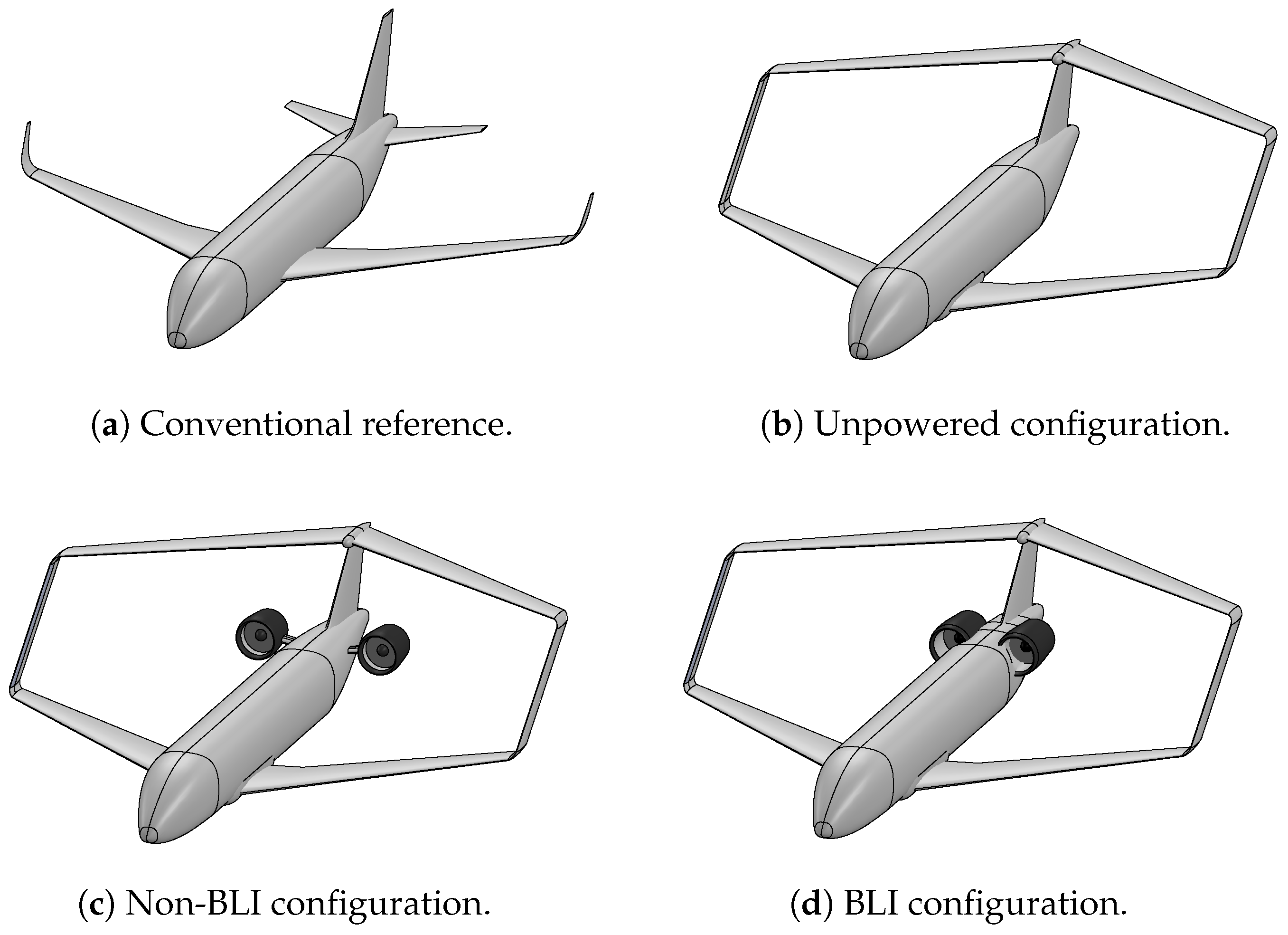
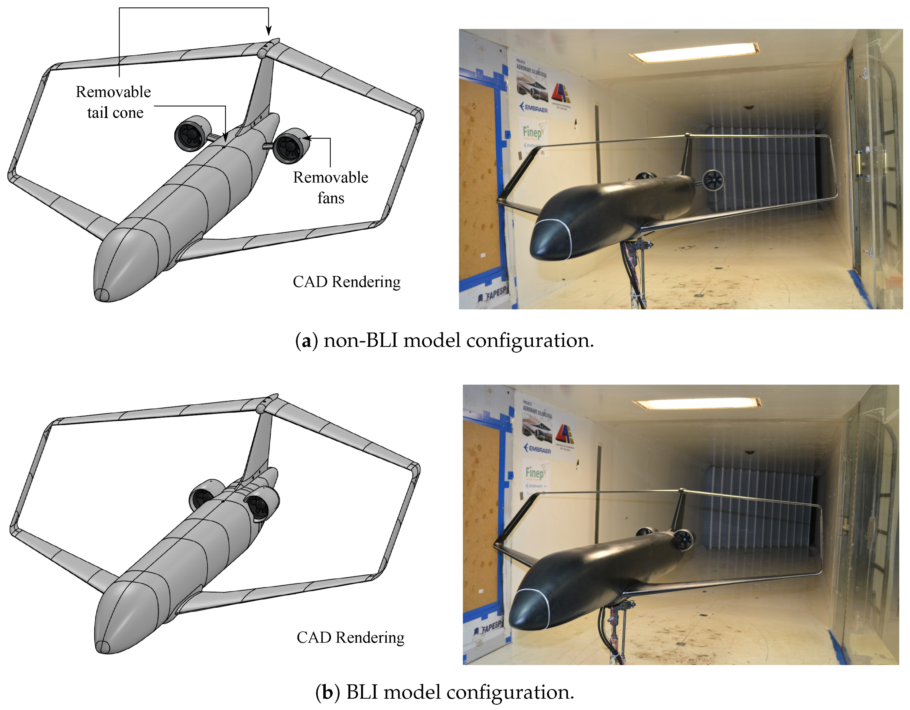
3.2. Tested Configurations

The wind-tunnel tests required the use of three different models. The first model was an unpowered configuration designed to measure the primary aerodynamic characteristics of the airframe. Figure 3a provides a schematic illustrating the key dimensions of this model. The technical views and detailed information about the electric fan employed in the wind tunnel experiments can be seen in Figure 3b. The second model represented the non-BLI configuration (Figure 4a) incorporated podded engines with axisymmetric nacelles. These engines were mounted on pylons at the rear section of the aircraft to facilitate the ingestion of clean airflow. The third model corresponded to the BLI configuration (Figure 4b). In this design, the engines were positioned with a semi-buried arrangement at the rear of the aircraft. This configuration was specifically developed to capture a relatively large portion of the boundary layer that formed over the fuselage.

To ensure the appropriate performance of the box-wing model at the subsonic wind-tunnel test conditions, adjustments were made to the airfoils compared to the full-scale configuration. These modifications were necessary to achieve accurate behavior at the relatively low Reynolds numbers encountered in the wind-tunnel experiments. Two methods were employed to establish a correlation between the experimental results and the performance of the full-scale aircraft. Firstly, the lift coefficient equivalence was ensured by using suitable airfoils. Secondly, the boundary-layer transition was induced by implementing trip strips on all the surfaces of the model, including the wings, fuselage, tail, and propulsor nacelles. The positioning and dimensions of the trip strips were determined to maintain a uniform increase in the drag coefficient as the wind tunnel speed decreased. This approach, recommended by Barlow et al. [29], was aimed to ensure the presence of fully turbulent boundary layers on the model under representative conditions. Grit size trip strips measuring 3 mm in width and 0.08 mm in thickness were applied across the entire aircraft model. For the closed-wing system, trip strips were positioned at $x/c=0.05$ on the suction side and at $x/c=0.10$ on the pressure side. As for the fuselage and nacelles, the trip strips were located at 5–10% of the body length. These adjustments were carefully determined to promote the development of fully turbulent boundary layers during the experimental campaign, thereby aligning the model’s behavior with that of the full-scale aircraft. For more detailed information about the experimental model breakdown, see [27].

The models were fabricated by utilizing additive manufacturing methods that employed advanced techniques in the production process. A total of 48 individual pieces were created to construct the mockups, with carbon fiber beams utilized to reinforce the structure of the closed-wing configuration. These pieces were meticulously assembled by hand and adhered to the manufacturing tolerances derived from the computer-aided design (CAD) process. To ensure optimal aerodynamic performance, the surfaces of the models were treated and painted, thus resulting in a smooth and refined surface finish. It is important to note that the non-BLI, BLI, and unpowered models shared identical physical components, with the exception of the removable tail cone. The connections between these components were adjustable, thereby allowing for precise alignment, and they were secured in place using set screws. Both the non-BLI and BLI models are equipped with two QF2827-2300 KV brushless motors, each featuring six blades. These motors are commonly used in remote-controlled (R/C) models. The central duct of the electric ducted fan (EDF) has an outer diameter of 70 mm and a total length of 58 mm. The nominal voltage range for the fan is 8–22 VDC, with a maximum allowed electrical current of 50 A. Each fan is capable of generating a maximum thrust of 16.77 N at a rotational speed of 30,000 RPM. To control the EDFs, a Readytosky 50 A electronic speed controller (ESC) was employed, while a RSP-3000-48 power supply provided the necessary electrical power. The rotational speed of the motor shaft was measured precisely using an optical tachometer that utilized a laser light. The speed controllers were housed within the fuselage of the model. To adjust the propulsor power, the fan wheel speed was controlled using a SIKAF RC servo speed controller.

3.3. Test Conditions

The LAE-1 wind tunnel was carefully operated at velocities of approximately 27 m/s and 30 m/s, which corresponded to Reynolds numbers based on the reference chord lengths of $2.72\times {10}^5$ and $3.02\times {10}^5$, respectively. These velocities were selected after thorough testing of the propulsor’s thermal capabilities and the structural limitations of the model, with the latter often being the constraining factor. Prior to each test, the atmospheric conditions were closely monitored to establish the necessary non-dimensional parameters. The atmospheric pressure was measured using a calibrated mercury barometer with a precision of 1 mmHg. The temperature inside the wind tunnel was measured using a thermocouple, and the relative humidity was determined with a hygrometer to calculate the air density. The dynamic pressure was measured with a pitot-static probe positioned at the test section, which was connected to a micro-manometer (TSI Model 8705 DEP-CALC) with an uncertainty of ±0.1 Pa. The model was securely installed on the pitch–strut system and remained in place throughout the entire test campaign. Changes to the tail cone and instrumentation of the fans were performed in situ as necessary. The reference quantities for the tunnel’s operating conditions can be found in

Table 1. Non-dimensional flow parameters for different tests.

Freestream	Dynamic	Mach	Reynolds
Velocity [m/s]	Pressure [Pa]	Number [-]	Number [-]
27.0	410.9	0.080	$2.72\times {10}^5$
30.0	507.3	0.089	$3.02\times {10}^5$

, while the non-dimensional fan wheel speeds implemented during the tests are presented in

Table 2. Propulsor dimensional and non-dimensional wheel speeds.

$\Omega$ [RPM]		9000	10,300	15,500	18,200	20,400
$U_{tip}/V_{\infty }$ [-] at	$V_{\infty }\approx 27.0\mathrm{m}/\mathrm{s}$	1.33	1.44	2.17	2.55	2.86
	$V_{\infty }\approx 30.0\mathrm{m}/\mathrm{s}$	1.20	1.30	1.96	2.30	2.58

. The ratio between the fan blade tip speed and the tunnel speed ($U_{tip}/V_{\infty }$) was used to assess the effect of the propulsors on the flow features, where the fan blade tip speed is defined by Equation (1):

$$U_{tip}={\Omega }_f\frac{d_{fan}}{2}$$

(1)

where ${\Omega }_f$ is the fan wheel speed, and $d_{fan}$ is the model propulsor fan diameter, which is equal to 73 mm.

3.4. Data Collection

Four main types of runs were performed:

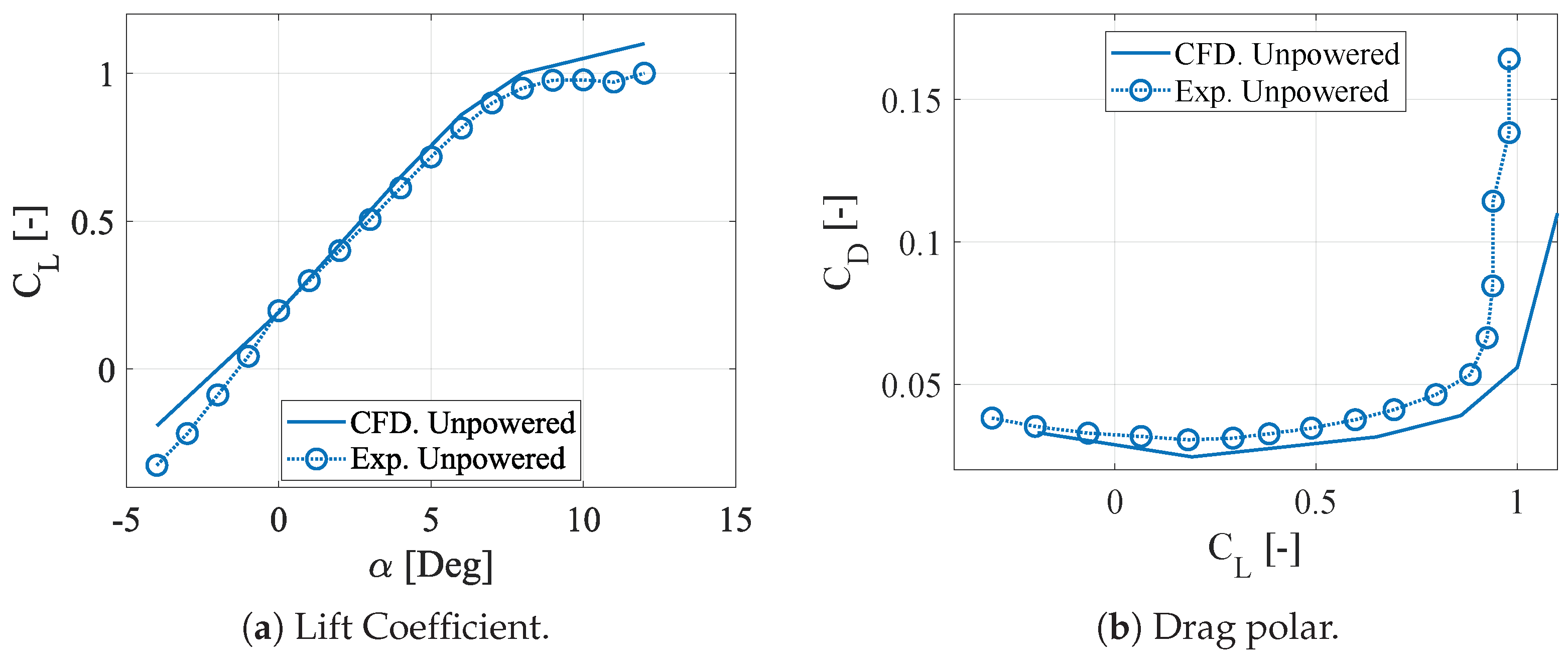
• Aerodynamic force measurements, including lift and drag, were conducted on the unpowered, non-BLI, and BLI configurations to assess their aerodynamic characteristics at various angles of attack ($\alpha$). To isolate the effects of geometry, the engines were easily removed from the nacelle, thus creating conditions simulating through-flow nacelles. This approach enabled the analysis of the pure geometric influences on the aerodynamics. For the unpowered configuration, the wind-tunnel results were compared to CFDs simulations to provide a form of experimental validation. The angles of attack tested ranged from $\alpha =-4^{\circ }$ to ${12}^{\circ }$ in increments of $1^{\circ }$.
• Measurements of the electrical power ($P_E$) were conducted on the non-BLI and BLI models. The objective of this experiment was to determine the electrical power coefficient and the net stream-wise force ($F_X$) for a range of fan wheel speeds, with a fixed angle of attack and tunnel velocity. A set of pre-determined fan wheel speeds was defined, and force and power readings were collected. The product between the voltage input to the ESC (v) and the current from the power supply (i) determined the electrical power supplied to the propulsors ($P_E=vi$).
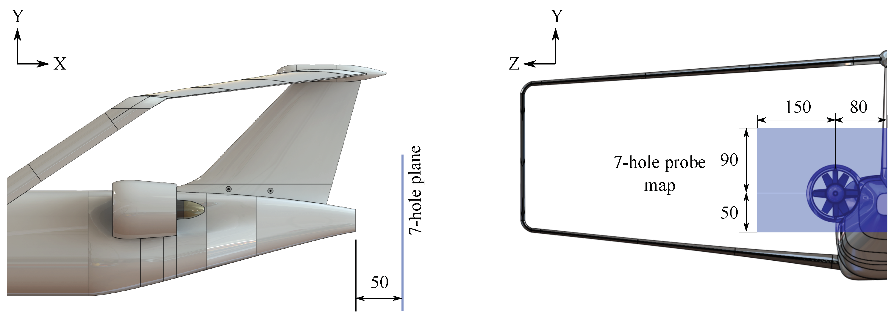
• Flow field measurements were performed on both the powered and unpowered models. The objective was to analyze the variation of the axial flow velocity ($u^{*}$) across different configurations in a transversal plane. To achieve this, the aerodynamic measurements focused on presenting the stream-wise velocity contours and flow mapping at selected fan wheel speeds, with a fixed angle of attack and tunnel velocity. In the case of the powered configurations, the flow surveys were conducted at power levels that encompassed the range of zero net stream-wise force. This allowed for a comprehensive understanding of the flow characteristics and their relationship to the propulsive performance of the models.
• Measurements of the inlet pressure distortion were conducted on the models without the fan installed to assess the influence of the airframe on the distortion levels across different points in the flight envelope. The objective was to compare the distortion levels between a non-BLI configuration and a BLI configuration. To achieve this, total pressure rake surveys were performed at a fixed tunnel velocity while varying the angle of attack within the range of $0^{\circ }$ to $8^{\circ }$ in $1^{\circ }$ increments. This allowed for a comprehensive analysis of the dependence of the distortion on the airframe and provided insights into the differences between the non-BLI and BLI configurations.

3.5. Measurement Techniques

3.5.1. Aerodynamic Forces

A two-component balance was utilized to measure the aerodynamic forces acting on the models, as depicted in detail A of Figure 2. The drag balance was constructed in the Laboratory of Experimental Aerodynamics at EESC—USP. Conversely, the lift force was measured using a second balance consisting of two strain gauges positioned on flexure stiffeners, thus forming a Wheatstone bridge. Additional information regarding the lift balance and the angle of attack control mechanism can be found in the work by Cerón-Munoz [30], while previous aerodynamic results obtained using the current balance configuration can be found in [31,32]. The signals from the balances were recorded using a data acquisition sheet, specifically, the NI AT-M10-16X, with a sampling frequency of 500 Hz. Prior to the experiments, the aerodynamic balances were calibrated by applying known weights to establish a linear voltage–force relationship. The complete setup achieved a measurement accuracy of up to +0.7% under maximum loading conditions. Therefore, the accuracies for the lift, drag, and angle of attack measurements were approximately $\pm 0.8\mathrm{N}$, $\pm 0.18\mathrm{N}$, and $0.2^{\circ }$, respectively (see Appendix A).

The net stream-wise force can be defined as the difference between the drag and thrust [12], which is positive in the downstream direction. In its non-dimensional form, the net stream-wise force coefficient ($C_X$) is expressed by the following:

$$C_X=\frac{T_{EDF}-D}{q_{\infty }S}=C_T-C_D$$

(2)

where $T_{EDF}$ is the thrust generated by the EDFs, D is the drag of the model, $q_{\infty }$ is the freestream (tunnel) dynamic pressure, S is the wing reference area, $C_T$ is the thrust coefficient, and $C_D$ is the drag coefficient. In this case, the experiment was carried out in search of a zero net stream-wise force, which is calculated using the load cell of the drag balance to measure the difference between the propulsor’s gross thrust and the model’s drag. The pitch–strut system drag was subtracted from the model’s drag to determine the main aerodynamic characteristics of the aircraft. This process involved a simple approach to evaluate the tare (direct drag of the support), in which the forces on the pitch–strut system (i.e., removing the model) are measured at different tunnel speeds, and the drag generated by the support is corrected as a function of the tunnel dynamic pressure using regression statistical analysis [29].

To determine the primary aerodynamic coefficients, the wind tunnel data of the unpowered configuration was compared to CFDs simulations. The atmospheric conditions of the experimental setup were adjusted to the computational setup. Two computational domains with different sizes were considered: a small one to simulate the confined flow of the wind tunnel and a large one to simulate free-air conditions. The drag difference between these simulations was subtracted to the drag of the wind-tunnel model to account for wall effects. An unstructured tetrahedral mesh was used in all the simulations, as shown in Figure 5a. The grid density was regulated near the aerodynamic surfaces to increase the grid’s resolution in that region. The dimension of the cells in the refinement area was limited to $0.02\mathrm{m}$. The surface meshes were influenced by structured cells (prisms) in order to capture the boundary layer effects with adequate precision. The near-wall treatment was adjusted in terms of the total thickness, with 30 sub-layers and a growth rate of 1.2. The boundary layer refinement kept the dimensionless wall distance value (y+) close to 5.0. The generated mesh of the large domain featured a total of 6.32 million nodes. Figure 5b shows a pressure contour on the model surfaces. From these results, it was possible to determine the loads applied to the surface of the aircraft model. Consequently, in a more advanced design phase, the required structural strength of the internal layout and skin could be calculated.

The inlet velocity was set to 30 m/s, whereas the turbulent intensity was set to 0.21% based on the wind tunnel turbulence level [25]. On the symmetry plane of the domain, a symmetric boundary condition was applied, while the model surfaces were treated as no-slip walls. The outlet surface of the domain was modeled as a pressure outlet. Steady simulations using the SST turbulence model were carried out for the CFDs analysis. Second-order schemes were used for all the flow, i.e., the advection terms and turbulence numerics were discretized using a high-resolution scheme. The convergence control was set to reach 600 iterations, with a residual target equal to $1\times {10}^{-5}$.

3.5.2. Application of the Power Balance Equation

In this section, we derive the main equation of the power balance method, which is a solution introduced by Drela [16] for assessing the performance of tightly coupled systems. Unlike traditional approaches that rely on momentum equation analysis, the power balance method emphasizes the analysis of mechanical power and kinetic energy. Specifically, when considering a control volume that encompasses the propulsor and assuming low speeds, the power balance equation simplifies to only include the mechanical flow power ($P_K$) as the input power term. The mechanical flow power is calculated as follows:

$$P_K\equiv \left(p_{t\infty }-p_t\right)\mathbf{V}·\widehat{n}d\mathcal{S}$$

(3)

where $p_t$ and $\mathbf{V}$ represent the flow stagnation pressure and the local velocity vector, respectively, $\widehat{n}$ is the normal vector, which points into the propulsor, and $d\mathcal{S}$ is the surface differential. As stated by Uranga et al. [12], the mechanical flow power can be determined using two different methods: the direct method and the indirect method. The direct method involves conducting flow measurements at the inflow and outflow planes of the propulsor using techniques such as particle image velocimetry (PIV), a 5-hole probe, or a rotating $P_t$-rake system. On the other hand, the indirect method calculates the mechanical flow power based on the measured electrical power supplied to the motor in combination with the fan efficiency (${\eta }_f$) and motor efficiency (${\eta }_m$). These quantities can be made non-dimensional as follows:

$$C_{P_K}\equiv \frac{P_K}{q_{\infty }{V}_{\infty }S}$$

(4)

$$C_{P_E}\equiv \frac{P_E}{q_{\infty }{V}_{\infty }S}$$

(5)

$$C_{P_K}={\eta }_f{\eta }_m{C}_{P_E}$$

(6)

The BLI benefit is given by the power-saving coefficient (PSC), where the objective is to obtain the required power to achieve a zero net stream-wise force:

$$PSC\equiv \frac{{\left(C_{P_K}\right)}_{\mathit{non-BLI}}-{\left(C_{P_K}\right)}_{BLI}}{{\left(C_{P_K}\right)}_{\mathit{non-BLI}}}$$

(7)

In these experiments, it was assumed that the efficiencies of the fan and motor did not significantly differ between the BLI and non-BLI configurations at the same operating point. Preliminary motor characterization data from the EDF’s datasheet indicated that the motor operated close to its maximum efficiency, which was greater than 71%. Based on this information, the approach used in this study considered the motor operating near its maximum efficiency as a surrogate to evaluate the flow power. This allowed for the direct measurement of the electrical power during the wind-tunnel tests [33]. Therefore, it was assumed that the BLI benefit could be calculated using the following expression:

$$PSC\equiv \frac{{\left(C_{P_E}\right)}_{\mathit{non-BLI}}-{\left(C_{P_E}\right)}_{BLI}}{{\left(C_{P_E}\right)}_{\mathit{non-BLI}}}$$

(8)

Note that the assumption of maintaining constant efficiencies for the BLI benefit leads to higher uncertainty. In this case, the uncertainty in the BLI benefit was found to be $\pm 2.5\%$ (see Appendix B).

3.5.3. Flow Mapping

Flowfield measurements were conducted using a L-shape 7-hole probe, specifically, the AeroProbe^® system. This probe consists of a conventional cylindrical body made of stainless steel with a diameter of 3.2 mm and seven holes located at its tip. The design of the probe allows for accurate measurements in wind-tunnel testing, as the tip is directly exposed to the airflow, and the probe is mounted on the side to avoid the disruption of the data. With this probe, precise measurements of the flow vector magnitude, direction, static pressure, and total pressure can be obtained. The 7-hole probe has an acceptance angle of up to $\pm {30}^{\circ }$ with an error rate lower than $\pm 1^{\circ }$. The velocity error can also be kept below ±1%, and it offers up to 500 discrete aerodynamic calibration points per speed [34]. To ensure its accuracy, the calibration of the 7-hole probe was performed using a neural network trained with input data ranging from $\pm {30}^{\circ }$, with 1-degree precision in both the Y and Z directions. The root mean square (RMS) error achieved in the calibration process was 0.1 m/s. More details can be found in [27].

In order to obtain the wake characteristics, a three-axis traverse system, specifically the DANTEC^® traverse system, was employed to move the sensors in a pre-defined grid. This system allowed for precise movements of the probe in three directions, thus achieving micro-meter accuracy. Each axis movement had an accuracy of 0.0125 mm and was controlled through serial communication. The traverse system was positioned approximately 50 mm away from the fuselage tail cone, where a rectangular transversal plane was selected to measure the flow pattern of the propulsor jet. Using the center of the fan diameter as a reference, the grid of the rectangular transversal plane was defined from 150 mm to −80 mm with a spacing of 5 mm in the lateral direction, and from −50 mm to 90 mm with a spacing of 5 mm in the vertical direction.

To ensure accurate measurements, the data averaging process involved 500 samples obtained from 5 s measurements. The probe was traversed through the same grid points in both space and time. At each point, time-averaged values for the three velocity components ($u^{}$, $v^{}$, and $w^{*}$) and velocity fluctuations ($u_{rms}$, $v_{rms}$, and $w_{rms}$) were recorded. The in-plane velocity vectors ($v^{}$ and $w^{}$) were used to calculate the stream-wise vorticity (${\omega }_x$). The dimensions of the grid planes used for wake mapping can be seen in Figure 6, and the complete setup of the wake mapping experiment, mounted on the wind tunnel test section, is depicted in Figure 7.

3.5.4. Steady Total Pressure Distribution and Distortion Analysis

The inlet efficiency was evaluated through the total pressure coefficient (Equation (9)) and the distortion index (Equation (10)), which are defined as follows:

$$C_{p_t}=\frac{p_t-p_{t_{\infty }}}{q_{\infty }}$$

(9)

$$D{C}_{\theta }=\frac{p_{t_{AIP}}-p_{\theta }}{q_{AIP}}$$

(10)

where $p_{t_{AIP}}$ is the average total pressure value in the survey plane (${360}^{\circ }$), $p_{\theta }$ is the minimum average total pressure value in a sector of ${60}^{\circ }$, and $q_{AIP}$ is the mean dynamic pressure that is calculated by $q_{AIP}=\rho V_{AIP}^2/2$. The goal of these tests was to look inside the engine inlet duct and study if there was a significant difference in the overall pressure across the aerodynamic interface plane (AIP) between the configurations. The total pressure distribution at the AIP was measured with a total pressure rake with an outer diameter of 70.5 mm. The rake was located in a plane that was perpendicular to the freestream velocity direction, as shown in Figure 8.

The rake utilized in the experiment featured 40 total pressure probes, which were strategically placed in eight circumferential locations with a spacing of ${25}^{\circ }$ and five radial locations. The pressure data for each configuration and condition were collected using a pressure scanner (Scanivalve^® DS4-48) over a period of 5 s and averaged during this duration. The pressure scanner had a pressure rating ranging from 0.01 to 100 psi. The scanivalve employed an electro-mechanical pressure multi-plexer, which allowed for the sequential reading and transmission of multiple input signals using a solenoid. The position transmitter (encoder) electrically indicated the port being measured, while a solenoid stepper drive facilitated the sequential connection of the ports to 48 transducers. The signal conditioner gain was adjusted to match the full-scale pressure range of the transducer, which corresponded to a 5 v (20 mA) output [35]. Simultaneously, the freestream static and total pressures were measured using a pitot-static probe positioned at the inlet of the test section. These measurements were acquired using the same pressure scanner. By monitoring the freestream conditions, any potential variations due to the temperature or velocity drifts were taken into account. The measurement uncertainty for each type of run was estimated to be 1% (see Appendix B).

4. Results and Discussions

In this section, the experimental and CFDs results for the unpowered configuration are first analyzed and compared (Figure 9). Alpha sweeps (from $\alpha =-4^{\circ }$ to ${12}^{\circ }$ in $4^{\circ }$ steps) using the converged grid were run to better understand the offset from experimental data. Experimental force measurement results of the three configurations in through-flow nacelle conditions are also presented and discussed (Figure 10). Lift and drag coefficients, drag polar, and aerodynamic efficiency are the variables evaluated.

Table 3. Aerodynamic forces of the configurations in through-flow nacelle conditions at $M=0.089$ and $Re=3.02\times {10}^5$.

Configuration	Unpowered			Non-BLI		BLI
Parameter	Exp	CFD	% Error	Exp	$\Delta$ [%]	Exp	$\Delta$ [%]
$C_L$ for zero $\alpha$ [-]	$0.181\pm 0.0084$	0.191	5.52	$0.187\pm 0.0093$	$3.31\pm 0.11$	$0.184\pm 0.0097$	$1.65\pm 0.15$
$\partial C_L/\partial \alpha$ [-]	$0.102\pm 0.0118$	0.111	8.82	$0.102\pm 0.0106$	0.0	$0.102\pm 0.0113$	0.0
$C_{Lmax}$ [-]	$0.{985}_{{|}_{{11}^{\circ }}}\pm 0.0157$	$1.{092}_{{|}_{{12}^{\circ }}}$	10.86	$0.{997}_{{|}_{{10}^{\circ }}}\pm 0.0138$	$1.21\pm 0.12$	$1.{004}_{{|}_{{10}^{\circ }}}\pm 0.0149$	$1.92\pm 0.10$
$C_D$ for zero $\alpha$ [-]	$0.0304\pm 0.0042$	0.0245	19.40	$0.0338\pm 0.0064$	$11.18\pm 0.52$	$0.0319\pm 0.0051$	$4.93\pm 0.21$
$\partial C_D/\partial C_L^2$ [-]	$0.0217\pm 0.0107$	0.018	14.28	$0.0226\pm 0.0101$	$4.14\pm 0.05$	$0.0224\pm 0.0099$	$3.03\pm 0.07$
${(L/D)}_{max}$ [-]	$17.{21}_{{|}_{6^{\circ }}}\pm 0.0098$	$22.{05}_{{|}_{6^{\circ }}}$	28.12	$15.{77}_{{|}_{6^{\circ }}}\pm 0.0010$	$8.36\pm 0.89$	$16.{67}_{{|}_{6^{\circ }}}\pm 0.0088$	$3.13\pm 0.10$

shows a summary of the results from the experimental–numerical comparison of the unpowered configuration, as well as the differences between the experimental curves of the configurations.

Figure 9a shows the comparison of lift coefficient as a function of the angle of attack. The lift curves show correlations for low to moderate angles of attack between the two methods, since the curves displayed a linear behavior with a similar slope ($\partial C_L/\partial \alpha$) from $\alpha =$ $0^{\circ }$ to $5^{\circ }$ (See Table 3). However, the CFDs results over-predicted the lift at negative angles. This could be explained by the fact that the wind-tunnel models had strips on both sides of the wing section, thereby artificially increasing the boundary-layer thickness and reducing the model’s effective curvature. Note that a greater dispersion (in the order of 11%) at high angles of attack was found due to the higher level of complexity in the flow pattern arising from the stall region, which was more difficult to be numerically simulated. Despite the fact that the $C_L-\alpha$ curve matched well among all the simulations, there was an offset from the experimental data by approximately $-0.3^{\circ }$ in the angle of attack. This can be seen in Table 3, where the $C_L$ for the zero $\alpha$ had an error of 5.52%, which was explained by the calculated uncertainty of the pitch–strut system, i.e., the effective angle of attack of the wind-tunnel model might have been higher than the geometric angle of attack. At this point, additional investigations are needed to determine the reason for the shift.

Figure 9b depicts the complete drag-polar chart for the unpowered configuration. The CFDs results show under-predictions with the experimental data in all the evaluated angles of attack, where the values at the zero angle of attack were 0.0245 and 0.0304, respectively (error rate of 19.4%). Although there was an offset in the drag levels between the fully turbulent computation and the experimental data, the curves showed relatively good agreement at low to moderate angles of attack. It should be noted that increasing the grid density will result in a better approximation of the numerical data in terms of the $C_D$. On the other hand, the experimental curve showed larger drag values as the angle of attack increased. The reason for that difference was due to vibrations of the model under the effect of stall detachments, thereby increasing the predicted drag values.

The experimental results of the unpowered configuration, as well as the non-BLI and BLI configurations in through-flow nacelle conditions, are presented in Figure 10. According to the lift coefficient results (Figure 10a), the nacelle induced a gradually increasing amount of extra lift between $\alpha =0^{\circ }$ and $\alpha =5^{\circ }$; however, the change in lift was relatively small. At high angles of attack (i.e., from $\alpha =8^{\circ }$ to $\alpha ={12}^{\circ }$), the configurations exhibited a smooth stall behavior, which can be explained by the mutual interaction of the wings, in which the aft wing continues to provide lift, while the fore wing has already started the stall process. As a result, in the post-stall regime, the lift coefficient did not drop rapidly, thus resulting in a nose pitch-down tendency. Such a characteristic allowed the BW concepts to avoid risks due to a stall effect when approaching the stall angle, thus maximizing the total lift without creating adverse trim effects. This has a significant impact on safety, especially in commercial aircraft categories. This behavior was also observed in the IDINTOS project, where low-speed wind-tunnel results showed the mutual interference between the wings, which changed at different angles of attack [36]. The mini-tuft flow visualization technique applied on the main box-wing surfaces near stall conditions also confirmed this behavior (Figure 11). The mini-tufts indicated a region of blurred tufts flow on the fore wing, whereas the flow on the aft wing was completely unseparated.

The impact of the through-flow nacelles on the overall aircraft drag was also evidenced by comparing the experimental curves (Figure 10b). As expected, the non-BLI configuration showed an increase in the total drag due to the contribution of pylons, as well as the contribution of nacelle drag. The mutual aerodynamic interference between the pylon and the nacelle increased the drag by about 11% in comparison with the unpowered configuration. In contrast, the BLI configuration increased the drag in the order of 5% compared to the unpowered configuration, thus indicating that the magnitude of the interference drag of the BLI model was lower than the non-BLI model, i.e., the BLI model allowed for smaller nacelles and eliminated the pylons, thus reducing the total wetted area and, consequently, the surface dissipation.

Figure 10c illustrates the drag-polar chart. Clearly, the through-flow nacelles can have a notable impact on the overall changes in $C_D$, but the three configurations exhibited nearly the same $C_L$ over the operating range of $\alpha$ between $2^{\circ }$ and $6^{\circ }$. This result is easier to understand in Table 3, where the variation in the drag coefficient with the square of the lift coefficient ($\partial C_D/\partial C_L^2$) is presented (the induced drag parameter). The lift properties and span-wise load distributions were substantially identical for all the configurations, which means that the BLI and non-BLI configurations had the same vortex dissipation, thus implying that only propulsion aerodynamic factors contributed to the BLI benefit.

Figure 10d shows the aerodynamic efficiency curves versus the lift coefficient. All configurations displayed a similar pattern, where the maximum values were obtained between the interval $0.5\le C_L\le 0.8$, which corresponds to $4^{\circ }\le \alpha \le 6^{\circ }$. The efficiency curves showed that the drag increase was produced by the mounted nacelles. Note that the aerodynamic performance of the non-BLI and BLI configurations decreased by 8.36% and 3.13%, respectively, when compared to the unpowered configuration. For the sake of argument, it can be concluded that all the aerodynamic measurements were performed successfully, since the specific characteristics about the performance of this particular unconventional configuration were observed, such as the soft stall induced by the closed-wing system, as well as the viscous drag increase caused by the pylon/nacelle interference.

4.1. Power Balance and BLI Benefit

The outcomes of the integrated systems (non-BLI and BLI configurations) are provided in this section. At Reynolds numbers of $2.72\times {10}^5$ and $3.02\times {10}^5$, the wheel speed of the propulsors were varied, and the net stream-wise force and electrical power were measured. The results are shown in Figure 12, where the net stream-wise force coefficient (defined in Equation (2)) is plotted against the electrical power coefficient (defined in Equation (5)). The crosses represent the points for the seven different runs, and the lines are the cubic splines that were curve-fit through the average of these points at each motor speed (

Table 4. Cubic curve fits of the $C_{P_E}$ versus $C_X$ data.

Tunnel Condition	Configuration	Curve Fits and Confidence Interval
$R_e=2.72\times {10}^5$	non-BLI	$y=2.6x^3+0.5574x^2-0.6947x+0.03609$; $R^2=0.999$
$R_e=3.02\times {10}^5$	non-BLI	$y=3.6x^3+0.4454x^2-0.6983x+0.03689$; $R^2=0.999$
$R_e=2.72\times {10}^5$	BLI	$y=10.8x^3-0.989x^2-0.5878x+0.03$; $R^2=0.997$
$R_e=3.02\times {10}^5$	BLI	$y=-0.65x^3+1.292x^2-0.7276x+0.03364$; $R^2=0.998$

). Across the entire range of the power levels evaluated (Figure 12a), the BLI configuration required less electrical power for a given net stream-wise force than the non-BLI configuration. The BLI benefit (defined in Equation (8)) at $C_X=0$ was found to be $PSC=7.41\pm 2.5\%$. Such data were obtained by adjusting the electrical power of the EDFs until the net axial force on the apparatus was zero, as measured by the load cell. The data were averaged to evaluate how the engine thrust and nacelle installation affected the power measurements in the non-BLI and BLI configurations. These points can be seen in the zoomed-in view in Figure 12b. The results were comparable to previous experimental studies that employed the electrical power coefficient instead of the mechanical flow power coefficient. For example, Uranga et al. [33] reported preliminary experimental analyses of the double-bubble D8 aircraft with a focus on the differences between the BLI and non-BLI configurations at a Reynolds number of $3.6\times {10}^5$. The authors found a BLI benefit of about $6.85\pm 2.3\%$. This result is highly comparable to subsequent experiments on this aircraft, in which the measurements of the pressure fields, velocity magnitudes, and flow directions were used to calculate the mechanical flow power of the propulsors [12]. In the latter case, the measured BLI benefit was $8.6\pm 1.8\%$ at a simulated cruise. Given the experimental uncertainty, the application of the electrical power coefficient under the premise that the motor and fan worked near peak efficiencies did not reveal substantial variance, as a positive advantage was found in both experimental campaigns.

On the other hand, the CFDs simulations using the actual scale and flight conditions of the aircraft demonstrated a power-saving coefficient of about 6.52%, as shown in [22]. This result is not plotted in Figure 12, because it cannot be compared directly to the power extracted from the wind tunnel experiments. The CFDs used an actuator disk model to characterize the propulsors, which did not consider the fan rotation. Although the raw experimental data had some uncertainty due to the large degree of interference among the numerous competing effects, it was determined that the studied propulsion system had the potential to provide specific BLI benefits in the order of 5% to 7%.

4.2. Seven-Hole Probe Measurements

According to Uranga et al. [18], three major parameters can influence the BLI benefit: the amount of dissipation ingested by the propulsors; the BLI installation efficiency in terms of surface dissipation reductions; and the propulsor jet velocity (typically set by the propulsor mass flow). As shown in Figure 12, the variations in the $P_E$ between the configurations were derived from changes in the isolated airframe drag values, as well as the propulsion airframe integration effects. This confirms that the BLI benefit depends on the specifics of the integration between the propulsor, fuselage, and vertical tail, thereby achieving a reduction in the surface dissipation. However, the mechanical flow power, given by Equation (3), is dependent on the total pressure difference and the axial flow velocity, i.e., the stream-wise velocity, reflects the velocity deficit of the ingested boundary layer. In this context, seven-hole probe surveys were conducted as close as possible to the propulsors to investigate the flowfield downstream from the aircraft models. The axial velocity and stream-wise vorticity were the most relevant flow parameters in the study of the flowfield. Contour maps of the velocity ($u^{*}$) and stream-wise vorticity (${\omega }_x$) are shown in Figure 13 and Figure 14, respectively.

The velocity maps (Figure 13) show the difference between the through-flow nacelle condition (left) and the powered configurations (right) for non-BLI (Figure 13a) and BLI (Figure 13b) configurations, respectively. The contour maps for the $u^{*}$ component in the through-flow nacelle condition revealed regions of reduced velocity, which corresponded to the wake and velocity deficit of the airframe. The contour of the non-BLI configuration evidenced a clear aerodynamic interference between the pylon and nacelle, thus resulting in separation and increased drag on the nacelle’s surfaces. At that region, the lowest velocity reached approximately $0.9V_{\infty }$. In contrast, the contour of the BLI configuration exhibited a larger region of low-velocity fluid due to the incoming boundary layer. In this case, the lowest velocity value reached $0.83V_{\infty }$. In both cases, the wake from the tail cone had most likely merged, thus creating a large momentum deficit. On the other hand, the contour maps for the $u^{*}$ component in the powered configurations perceived the reduction in kinetic energy dissipation due to the wake and the propulsive jet. Note that the BLI configuration achieved a lower jet velocity ($1.03V_{\infty }$) than the non-BLI configuration ($1.08V_{\infty }$), because the exhaust velocities of the BLI propulsor had lower stagnation pressures than the non-BLI propulsor. This result explains the smaller amount of energy (electrical power) needed by the BLI configuration to reach a certain net stream-wise force.

The distributions of the axial vorticity along with velocity vectors for the non-BLI and BLI configurations are reported in Figure 14a,b, respectively. Both configurations exhibited a region of negative (clockwise) vorticity at the center, as well as positive structures along the trailing edges of the nacelles. Such vortical structures also come from the secondary flow resulting of the cross-sectional changes of the different airframes. However, the presence of fans imposed additional complexities, and the vortical structures are the result of the mixing of secondary flows with fan rotational motion. Despite very similar patterns being observed with lower fan voltage inputs, the BLI configuration presented a lower velocity magnitude than the non-BLI configuration when viewed from downstream.

4.3. Inlet Efficiency

The inflow distortion associated with the fuselage boundary layer is ingested by the inlet duct and delivered to the engine. This fact imposes compatibility challenges due to the effect of the distorted propulsor inflow on fan performance, thereby reducing the overall BLI benefit. To illustrate this issue, the total pressure coefficient contours, as well as the distortion analysis, can be seen in Figure 15. The grids for the total pressure survey were created using the locations of the probes mounted on the rake (Figure 8). Therefore, the total pressure coefficient contours were obtained by linearly interpolating in the radial and circumferential directions for the grid points between the innermost and outermost points on the survey grid. The values of $D{C}_{\theta }$ for both configurations and the number of runs lay within 1% of each other, thus confirming the repeatability of the measurements.

The ingested boundary layer can be noted clearly, wherein it presented high indices of distortion as a consequence of the reduced low-pressure region. However, as the angle of attack increased until $\alpha =8^{\circ }$, the performance variation of the BLI configuration was relatively low. Note that the pressure distribution seemed similar, and the difference in distortion between $\alpha =0^{\circ }$ and $\alpha =8^{\circ }$ was 5.9%. This indicates that changing the angle of attack had no significant effect on the cross-flow or separation in the current engine location, thereby implying that the fan performance should be unaffected under several flight conditions. In contrast, a clean airflow was evidenced for the non-BLI configuration until $\alpha =7^{\circ }$; however, at higher angles of attack, a small vortex was formed coming in from the side, thus creating distortion regions of lower total pressure in the aerodynamic interface plane. In sum, the non-BLI configuration presented distortion values of $D{C}_{\theta }\sim 0.004-0.007$ at low to moderate angles of attack, whereas the BLI configuration had distortion values of $D{C}_{\theta }\sim 0.021-0.023$ that corresponded to total pressure recovery values of ${\eta }_R=0.984\sim 0.977$ and ${\eta }_R=0.651\sim 0.613$, respectively. This indicates that further research is needed to determine the fan response (aerodynamic and aeromechanic) to these higher distortion levels, as well as the influence on the engine life cycle.

Finally, mini-tuft flow visualization was performed upstream and downstream of the nacelles to visualize the flow entering the propulsors. The arrangement of the mini-tufts at $\alpha =3^{\circ }$ is displayed in Figure 16 for both configurations. Although no large-scale separation can be identified, cross-flow can be seen in both configurations. There are some blurred tufts around the nacelle lips of the non-BLI configuration, thus indicating a region of accelerated flow. However, the flow far from the propulsors was steady, with the tufts all pointing in the flow direction. In contrast, separated flow can be seen around the incoming flow of the BLI configuration, with tufts pointing in a random direction and continuing inwards and towards the propulsor inlet, i.e., they indicated blockage and lower velocity flow entering to the propulsor, which caused high distortion levels. In this case, the overall flow over the nacelles remained aligned to the flow direction. In conclusion, inlet flow distortion is expected to play a major role in unconventional aircraft where complex air induction systems are required to couple the airframe with engines.

Two experimental setups were employed to investigate the aerodynamic interaction of the box-wing layout with the propulsion system: one focusing on the effect of podded engines on the airframe and one investigating boundary-layer ingestion inlets. The experimental data were used to validate preliminary CFDs studies [22], which were in turn used to perform sensitivity studies and complement the low-fidelity design of the concept. The experimental study included force and electrical power measurements, flow mapping, and total pressure surveys. The main results suggested that the BLI configuration enhanced the propulsive efficiency by reducing both the electrical power coefficient and the kinetic energy waste due to lower jet velocities. Other benefits included a reduced ram drag, lower structural weight, and a less wetted area than the pylon-mounted engine configuration. However, the propulsion–airframe integration of the BLI inlets introduces complicated aerodynamic interactions, thereby causing high levels of fan–face distortion that decrease engine performance and can lead to issues in the reliability of safe operation. Distortion further leads to additional vibration and noise; therefore, the optimum design of the airframe shape and the integration of distortion tolerant fan blades that adjust the boundary-layer ingestion are key elements for improving inlet/engine compatibility. The experimental results also confirmed that the box-wing concept is attractive for security reasons. In particular, the concept had a favorable stall recovery, in which the downwash on the aft wing was alleviated, thereby producing a soft stall and inducing a nose-down pitching moment to restore the state of the aircraft.

5. Conclusions

The wind-tunnel testing of a 3.5%-scale model of a new aircraft concept at the Laboratory of Aerodynamics of the Aeronautical Engineering Department from São Carlos School of Engineering—University of São Paulo has yielded significant insights into the aerodynamic benefits of boundary-layer ingestion. The following key findings were obtained:

• The analysis revealed a clear correlation between jet velocity and the power-saving coefficient due to BLI. The utilization of BLI enabled a lower jet velocity by ingesting slower flow, thus resulting in reduced momentum flow through the propulsor and more efficient power usage. The measurements demonstrated a minimum power saving of 7.41% ± 2.5% compared to conventional freestream flow ingesting configurations, with a 99% confidence interval. However, due to scale model limitations, the BLI benefit was quantified using electrical power instead of mechanical flow power measurements. Subsequent experiments will address this by converting the electrical power into mechanical flow power, thereby incorporating shaft and fan efficiencies.
• While the analysis did not explicitly evaluate the BLI benefit for an actual transonic transport aircraft, it did establish the processes necessary for evaluating the BLI’s potential on real aircraft geometries. This enables the integration of novel propulsion technologies with the airframe. The experiment’s results align closely with steady CFD-RANS simulations of the aircraft at actual scale and flight conditions, with a margin of error of ±2.5% due to aerodynamic modeling uncertainties.
• These results contribute to our understanding of BLI aerodynamics for several reasons. Firstly, the fan was appropriately scaled to match the full-scale fuselage boundary layer. Secondly, the utilized power balance method does not account for differences in the Reynolds and Mach numbers, and the BLI benefits primarily stemmed from a lower jet-to-freestream velocity ratio (reduction of approximately 4.63%) and reduced external losses due to a smaller nacelle wetted area (reduction of around 5.62%) compared to the non-BLI configuration. Thirdly, previous research suggests that compressibility effects have a minimal impact on the fuselage boundary layer. This demonstrates the efficacy of the current aerodynamic model experiment in assessing the aero-propulsive efficiency of a BLI aircraft configuration.
• The aerodynamic flow measurements confirmed the presence of flow distortion, which restricts the aerodynamic performance of the BLI configuration. Further investigations should focus on understanding the specific response of the fan to this distortion, thus considering material limitations and potential issues related to the noise and vibration caused by nonuniform incoming flow.
• Flow measurements were taken using a seven-hole probe. The probe’s interference with the flow warrants additional investigation, and the use of non-intrusive flow measurement techniques such as particle image velocimetry (PIV) can provide a comprehensive assessment of the flow field. While this research provides direct evidence of the benefits of boundary-layer ingestion, further studies are necessary to fully comprehend its influence on aircraft performance during detailed design phases.
• It is important to note that the experiments were conducted at lower Reynolds numbers and subsonic conditions when compared to actual flight. Therefore, it is essential to consider that the performance coefficients may differ in a full-scale application. More detailed research focusing on flight conditions will enable a more accurate comparison of different configurations.

References

1. Bravo-Mosquera, P.D.; Catalano, F.M.; Zingg, D.W. Unconventional aircraft for civil aviation: A review of concepts and design methodologies. Prog. Aerosp. Sci. 2022, 131, 100813. [Google Scholar] [CrossRef]
2. Moirou, N.G.; Sanders, D.S.; Laskaridis, P. Advancements and prospects of boundary layer ingestion propulsion concepts. Prog. Aerosp. Sci. 2023, 138, 100897. [Google Scholar] [CrossRef]
3. Brelje, B.J.; Martins, J.R. Electric, hybrid, and turboelectric fixed-wing aircraft: A review of concepts, models, and design approaches. Prog. Aerosp. Sci. 2019, 104, 1–19. [Google Scholar] [CrossRef]
4. Braga, D.F.; Tavares, S.; Da Silva, L.F.; Moreira, P.; De Castro, P.M. Advanced design for lightweight structures: Review and prospects. Prog. Aerosp. Sci. 2014, 69, 29–39. [Google Scholar] [CrossRef]
5. Liebeck, R.H. Design of the blended wing body subsonic transport. J. Aircr. 2004, 41, 10–25. [Google Scholar] [CrossRef] [Green Version]
6. Okonkwo, P.; Smith, H. Review of evolving trends in blended wing body aircraft design. Prog. Aerosp. Sci. 2016, 82, 1–23. [Google Scholar] [CrossRef]
7. Cavallaro, R.; Demasi, L. Challenges, ideas, and innovations of joined-wing configurations: A concept from the past, an opportunity for the future. Prog. Aerosp. Sci. 2016, 87, 1–93. [Google Scholar] [CrossRef]
8. Abu Salem, K.; Cipolla, V.; Palaia, G.; Binante, V.; Zanetti, D. A physics-based multidisciplinary approach for the preliminary design and performance analysis of a medium range aircraft with box-wing architecture. Aerospace 2021, 8, 292. [Google Scholar] [CrossRef]
9. Gur, O.; Bhatia, M.; Schetz, J.A.; Mason, W.H.; Kapania, R.K.; Mavris, D.N. Design optimization of a truss-braced-wing transonic transport aircraft. J. Aircr. 2010, 47, 1907–1917. [Google Scholar] [CrossRef]
10. Bradley, M.K.; Droney, C.K.; Allen, T.J. Subsonic Ultra Green Aircraft Research: Phase II. Volume 1; Truss Braced Wing Design Exploration; Technical Report; National Aeronautics and Space Admin Langley Research Center: Hampton, VA, USA, 2015.
11. Drela, M. Development of the D8 transport configuration. In Proceedings of the 29th AIAA Applied Aerodynamics Conference, Honolulu, HI, USA, 27–30 June 2011; p. 3970. [Google Scholar]
12. Uranga, A.; Drela, M.; Greitzer, E.M.; Hall, D.K.; Titchener, N.A.; Lieu, M.K.; Siu, N.M.; Casses, C.; Huang, A.C.; Gatlin, G.M.; et al. Boundary layer ingestion benefit of the D8 transport aircraft. AIAA J. 2017, 55, 3693–3708. [Google Scholar] [CrossRef]
13. Menegozzo, L.; Benini, E. Boundary layer ingestion propulsion: A review on numerical modeling. J. Eng. Gas Turbines Power 2020, 142, 120801. [Google Scholar] [CrossRef]
14. Seitz, A.; Habermann, A.L.; Peter, F.; Troeltsch, F.; Castillo Pardo, A.; Della Corte, B.; Van Sluis, M.; Goraj, Z.; Kowalski, M.; Zhao, X.; et al. Proof of concept study for fuselage boundary layer ingesting propulsion. Aerospace 2021, 8, 16. [Google Scholar] [CrossRef]
15. Carter, M.B.; Campbell, R.L.; Pendergraft, O.C., Jr.; Friedman, D.M.; Serrano, L. Designing and testing a blended wing body with boundary-layer ingestion nacelles. J. Aircr. 2006, 43, 1479–1489. [Google Scholar] [CrossRef] [Green Version]
16. Drela, M. Power balance in aerodynamic flows. AIAA J. 2009, 47, 1761–1771. [Google Scholar] [CrossRef] [Green Version]
17. Hall, D.K.; Huang, A.C.; Uranga, A.; Greitzer, E.M.; Drela, M.; Sato, S. Boundary layer ingestion propulsion benefit for transport aircraft. J. Propuls. Power 2017, 33, 1118–1129. [Google Scholar] [CrossRef]
18. Uranga, A.; Drela, M.; Hall, D.K.; Greitzer, E.M. Analysis of the Aerodynamic Benefit from Boundary Layer Ingestion for Transport Aircraft. AIAA J. 2018, 56, 4271–4281. [Google Scholar] [CrossRef]
19. Della Corte, B.; van Sluis, M.; Veldhuis, L.L.; Gangoli Rao, A. Power Balance Analysis Experiments on an Axisymmetric Fuselage with an Integrated Boundary-Layer-Ingesting Fan. AIAA J. 2021, 59, 5211–5224. [Google Scholar] [CrossRef]
20. Della Corte, B.; van Sluis, M.; Gangoli Rao, A.; Veldhuis, L.L. Aerodynamic Performance of an Aircraft with Aft-Fuselage Boundary Layer Ingestion Propulsion. In Proceedings of the AIAA AVIATION 2021 FORUM, Virtual, 2–6 August 2021; p. 2467. [Google Scholar]
21. A320—Aircraft Characteristics Airport and Maintenance Planning. 2005. Available online: https://www.airbus.com/sites/g/files/jlcbta136/files/2021-11/Airbus-Commercial-Aircraft-AC-A320.pdf (accessed on 5 March 2021).
22. Bravo-Mosquera, P.D.; Cerón-Muñoz, H.D.; Catalano, F.M. Design, aerodynamic analysis and optimization of a next-generation commercial airliner. J. Braz. Soc. Mech. Sci. Eng. 2022, 44, 609. [Google Scholar] [CrossRef]
23. Bravo-Mosquera, P.D.; Chau, T.; Catalano, F.M.; Zingg, D.W. Exploration of box-wing aircraft concept using high-fidelity aerodynamic shape optimization. In Proceedings of the 33th Congress of the International Council of the Aeronautical Sciences, Stockholm, Sweden, 4–9 September 2022. [Google Scholar]
24. Catalano, F. The new closed circuit wind tunnel of the Aircraft Laboratory of University of São Paulo, Brazil. In Proceedings of the 24th International Congress of the Aeronautical Sciencies ICAS, Yokohama, Japan, 29 August–3 September 2004. [Google Scholar]
25. Santana, L.D.; Carmo, M.; Catalano, F.M.; Medeiros, M.A. The update of an aerodynamic wind-tunnel for aeroacoustics testing. J. Aerosp. Technol. Manag. 2014, 6, 111–118. [Google Scholar] [CrossRef]
26. de Almeida, O.; Catalano, F.M.; Pereira, L.T. Improvements of a Hard-Wall Closed Test-Section of a Subsonic Wind Tunnel for Aeroacoustic Testing. Int. J. Acoust. Vib. 2021, 26, 248–258. [Google Scholar] [CrossRef]
27. Bravo-Mosquera, P.D. Methodologies for Designing, Optimizing, and Evaluating Possible Unconventional Aircraft Configurations for Future Civil Aviation. Ph.D. Thesis, São Carlos School of Engineering, University of São Paulo, São Carlos, Brazil, 2022. [Google Scholar]
28. Hantrais-Gervois, J.L.; Piat, J.F.; Hantrais, J.L. A Methodology to Derive Wind Tunnel Wall Corrections from RANS Simulations; Integration: London, ON, Canada, 2012. [Google Scholar]
29. Barlow, J.B.; Rae, W.H.; Pope, A. Low-Speed Wind Tunnel Testing; John Wiley & Sons: New York, NY, USA, 1999. [Google Scholar]
30. Cerón-Muñoz, H. Estudo da Interferência Aerodinâmica do Sistema Motopropulsor em uma Aeronave do Tipo Blended Wing Body. Ph.D. Thesis, São Carlos School of Engineering, University of São Paulo, São Carlos, Brazil, 2009. [Google Scholar]
31. Ceron-Muñoz, H.; Catalano, F. Aerodynamic interference of power-plant system on a Blended Wing Body. In Proceedings of the 27th International Congress of the Aeronautical Sciences, Nice, France, 19–24 September 2010. [Google Scholar]
32. Cerón-Muñoz, H.; Diaz-Izquierdo, D.; Bravo-Mosquera, P.; Catalano, F.; De Santana, L. Experimental analyses of droop, wingtips and fences on a BWB model. In Proceedings of the 30th Congress of the International Council of the Aeronautical Sciences (ICAS 2016), Daejeon, Republic of Korea, 25–30 September 2016; pp. 25–30. [Google Scholar]
33. Uranga, A.; Drela, M.; Greitzer, E.; Titchener, N.; Lieu, M.; Siu, N.; Huang, A.; Gatlin, G.M.; Hannon, J. Preliminary experimental assessment of the boundary layer ingestion benefit for the D8 aircraft. In Proceedings of the 52nd Aerospace Sciences Meeting, New York, NY, USA, 14 January 2014; p. 0906. [Google Scholar]
34. Aeroprobe L-Shaped Probe. 2018. Available online: https://www.aeroprobe.com (accessed on 23 March 2022).
35. Scanivalve Corp. Scanivalve DS4-48—Pressure Scanner Module, Instruction and Service Manual; Scanivalve Corp: Liberty Lake, WA, USA, 1975. [Google Scholar]
36. Frediani, A.; Cipolla, V.; Oliviero, F. IDINTOS: The first prototype of an amphibious PrandtlPlane-shaped aircraft. Aerotec. Missili Spaz. 2015, 94, 195–209. [Google Scholar] [CrossRef]
Figure 1. General view of the designed configurations. Source: Bravo-Mosquera et al. [22].
Aerospace 10 00651 g001
Figure 2. Schematic views (side and front) of the aircraft model in the test section of LAE-1 wind tunnel; dimensions in meters.
Aerospace 10 00651 g002
Figure 3. Details of the unpowered model and electric fan equipping the wind-tunnel powered models; dimensions in millimeters. (a) Technical views of the wind-tunnel unpowered model. (b) Detailed drawings of the EDF for powered configurations.
Aerospace 10 00651 g003
Figure 4. Models: CAD rendering of mockups and photographs of the wind-tunnel setup assembled in the test section of the LAE-1 subsonic wind tunnel (scale 1:28).
Aerospace 10 00651 g004
Figure 5. Results of the proposed CFD methodology on the unpowered configuration.
Aerospace 10 00651 g005
Figure 6. Grid dimensions for wake mapping with 7-hole pitot probe; dimensions in millimeters.
Aerospace 10 00651 g006
Figure 7. Overview of the wake mapping experiment in the test section. (a) BLI configuration installed in LAE-1. (b) Close-up view of the probe installation for the non-BLI experiments at LAE-1.
Aerospace 10 00651 g007
Figure 8. Total pressure rakes installed on the wind-tunnel models.
Aerospace 10 00651 g008
Figure 9. Alpha sweep of CFD and experimental results for unpowered configuration at M = 0.089 and R e = 3.02 × 10 5 . Repeatability is Δ C L = 0.007 and Δ C D = 0.003 .
Aerospace 10 00651 g009
Figure 10. Alpha sweep of wind-tunnel configurations in through-flow nacelle conditions at M = 0.089 and R e = 3.02 × 10 5 comparing free-air lift and drag with corrected experimental data. Repeatability is Δ C L = 0.007 , 0.009 , 0.007 for unpowered, non-BLI, and BLI configurations, respectively. Repeatability is Δ C D = 0.003 , 0.004 , 0.004 for unpowered, non-BLI, and BLI configurations, respectively.
Aerospace 10 00651 g010
Figure 11. Mini-tuft flow visualization on the wing surfaces at M = 0.089 , R e = 3.02 × 10 5 , and α = 10 .
Aerospace 10 00651 g011
Figure 12. Net stream-wise force coefficient versus electrical power coefficient at C L = 0.51 . For each of the configurations, symbols are experimental measurements, and lines are curve-fit to data points. Repeatability is Δ C P E = 0.003 , 0.008 or equivalently Δ C X = 0.003 , 0.007 for non-BLI and BLI configurations, respectively.
Aerospace 10 00651 g012
Figure 13. Axial velocity contours at R e = 3.02 × 10 5 , C L = 0.51 , and U t i p / V = 1.96 . Through-flow nacelle condition (a) and powered configurations (b).
Aerospace 10 00651 g013
Figure 14. Close-up views of stream-wise vorticity contours and velocity vectors at R e = 3.02 × 10 5 , C L = 0.51 , and U t i p / V = 1.96 .
Aerospace 10 00651 g014
Figure 15. D C θ and C p t experimental results measured on the aerodynamic interface plane at M = 0.089 , R e = 3.02 × 10 5 , and α from 0 to 8 .
Aerospace 10 00651 g015
Figure 16. Mini-tuft flow visualization of fuselage and nacelles upstream of propulsor inlets at M = 0.089 , R e = 3.02 × 10 5 , and α = 3 .
Aerospace 10 00651 g016