Article

Airfoil Analysis and Optimization Using a Petrov–Galerkin Finite Element and Machine Learning

1
Instituto Superior Técnico, 1049-001 Lisboa, Portugal
2
LAETA/IDMEC, Instituto Superior Técnico, 1049-001 Lisboa, Portugal
3
LAETA/AEROG, Universidade da Beira Interior, 1049-001 Lisboa, Portugal
*
Author to whom correspondence should be addressed.
Aerospace 2023, 10(7), 638; https://doi.org/10.3390/aerospace10070638
Submission received: 23 June 2023 / Revised: 7 July 2023 / Accepted: 12 July 2023 / Published: 15 July 2023

Abstract

:
For the analysis of low-speed incompressible fluid dynamics with turbulence around airfoils, we developed a finite element formulation based on a stabilized pressure and velocity formulation. To shape the optimization of bidimensional airfoils, this formulation is applied using machine learning (TensorFlow) and public domain global optimization algorithms. The goal is to maximize the lift-over-drag ratio by using the class-shape function transformation (CST) parameterization technique and machine learning. Specifically, we propose equal-order stabilized three-node triangles for the flow problem, standard three-node triangles for the approximate distance function (ADF) required in the turbulence stage, and stabilized three-node triangles for the Spalart–Allmaras turbulence model. The backward Euler time integration was employed. An implicit time-integration algorithm was adopted, and a solution was obtained using the Newton–Raphson method. This was made possible in the symbolic form via Mathematica with the AceGen package. Three benchmarks are presented, with Reynolds numbers up to 1 × 10 7 , demonstrating remarkable robustness. After the assessment of the new finite element, we used machine learning and global optimization for four angles of attack to calculate airfoil designs that maximized C L / C D .

1. Introduction

Research on airfoil shape optimization with classical gradient-based methods has been published for nearly five decades [1]. With the advent of automatic differentiation algorithms for machine learning (see the review article [2]) and backpropagation, it became advantageous to use machine learning algorithms for problems where sensitivity analyses were intricate, see, e.g., [3].
For airfoil optimization, it is customary to use finite-volume software to perform the CFD analysis [4], but PINN has also been successfully adopted [5]. The finite element (FE) choice in this work is supported by the need to further increase the application range of the simulation to a fluid–structure interaction (FSI).
We focus on three main components in the approach: (i) airfoil parameterization, (ii) CFD discretization and time integration, (iii) and machine learning/optimization. In [6], a TLBO (teaching–learning-based) optimization algorithm was proposed for shape optimization. The authors used class-shape function transformation (CST) parameterization for 3D numerical tests. For CFD analysis, a finite-volume method was adopted. In the work by Deng and Yi [7], a machine learning algorithm was trained to generate pressure distributions. Their objective was analysis efficiency. Latin hypercubes and CST parameterization were adopted for 2D numerical tests. In the work by Du et al. [8], a convolutional neural network algorithm for airfoil design and performance prediction (DPCNN) was established, A Bézier representation of the airfoil geometry was adopted, and the UIUC database was adopted in the training process [9]. In [8], ANSYS Fluent software was used to analyze the aerodynamic performance of the airfoil. In that paper, optimization was performed in the machine learning framework to maximize the function denoted by the ratio of the lift coefficient to the drag coefficient C L / C D . In Hui’s study [10], reinforced learning was combined with multiobjective optimization. A constraint on the airfoil thickness was enforced to prevent the thinning observed in the current paper. A free-form deformation (FFD) algorithm was adopted for the shape motion and the CFL3D CFD code was employed for the simulations. In Karali et al. [11], a lifting line method was introduced for modeling and optimizing small unmanned vehicles. In a similar approach to that of this work, Karali et al. tested a range of angles of attack and provided a black box function for both analysis and optimization. TensorFlow functions and parameters are similar to other contributions, but only 250 epochs were used. In [12], a deep convolutional generative adversarial network was adopted, which produced more realistic airfoils than normal, and a detector of geometric abnormalities was introduced. FFD parametrization was adopted in [12], with the optimizer being a variant of the sequential quadratic programming (SQP) algorithm. Tyan et al. [13] proposed an inverse design deep neural network (IDNN), dimensional reduction, and the NACA four-series airfoil geometry representation via 2D examples. In an alternative approach to optimization, Xu [14] proposed machine learning (ML) for the adjoint-variable method. In a parallel line of developments, it is worth mentioning the work by Gutierrez et al. [15], which focused on the optimization of propellers for high-altitude pseudo-satellites. More sophisticated modeling approaches, such as physics-informed neural networks (PINNs) [16], have also been adopted. A review of the state of the art was provided by Li, Du, and Martins [17], who also discussed filtering and dimensional reduction techniques.
Here, we propose distinct approaches: the panel solver XFOIL [18] and the mixed-Finite Element software SIMPLAS [19] (developed by the first author). CST parameterization with 10 parameters was adopted for each airfoil, which was read from the UIUC database [9], and the control volume was meshed using Triangle [20]; both SIMPLAS and XFOIL produced the C L / C D values. Four values of the attack angle were tested for each airfoil: α = 0 , 1 . 25 , 2 . 5 and 5 . After this, the TensorFlow machine learning library was employed to produce a function that returned C L / C D from the 10 CST parameters. A dual annealing algorithm was then employed to estimate the optimized airfoil.
This paper, which is aimed at optimizing recreational aircraft airfoils, is organized as follows: Section 2 discusses the CST parameterization. Section 3 focuses on a RANS finite element formulation based on equal-order velocity/pressure interpolation and stabilization terms. This is a variant of the Petrov–Galerkin formulation, which was created by the first author. In Section 4, the Spalart–Allmaras transport equation for the eddy viscosity is described and discretized. The machine learning algorithm for the solution and optimization is described in Section 5. The results are presented in Section 6.

2. Parameterization

The parameterization of airfoil geometry, although not strictly required from the simulation perspective, reduces the required information needed to feed the machine learning algorithm [21]. Among the established parameterization algorithms, the cubic version of the CST [22] (class function/shape function transformation method) algorithm has been profusely adopted. Although CST is not suitable for all profiles in the repositories, the greatest advantages of CST are as follows: (i) it is applicable to 3D airfoils and (ii) it only requires a small number of parameters. The latter is of special importance, as only a small number of profiles are available in the databases [9]. For traditional optimization algorithms, see, e.g., [23], the CST parameterization is also commonly adopted due to its convenience. Figure 1 shows the essential nomenclature of an airfoil.
We directly implemented the CST functions proposed by Kulfan [22], which are capable of analytically defining a variety of airfoils with a reduced number of parameters. CST equations are based on a Bézier curve with an added class function term. Lower and upper surfaces are defined, respectively, by:
ζ l χ = χ 0.5 1 χ S l χ + χ Δ ζ l
ζ u χ = χ 0.5 1 χ S u χ + χ Δ ζ u
where ζ l is the upper surface, ζ u is the lower surface, Δ ζ u and Δ ζ L define the thicknesses of the trailing edge, and S u χ and S l χ are the shape functions obtained from the Bernstein polynomials, N u χ ( N u + 1 dimensional) and N l χ ( N l + 1 dimensional), for the upper and lower surfaces, respectively:
N l χ = , N l ! i ! N l i ! χ i 1 χ N l i , , i = 0 , , N l
N u χ = , N u ! i ! N u i ! χ i 1 χ N u i , , i = 0 , , N u
The dimensionless coordinates are defined by:
χ ζ = 1 c x z
where c represents the chord length, x represents the coordinate along the chord length, and z represents the coordinate along the profile thickness. We now use all nodal images of ζ l as ζ l N and of ζ u as ζ u N . Solving the NU and NL equations and applying the method of least squares, we obtain
A l = C l T · C l 1 · C l T · ζ l N χ l N Δ ζ l
A u = C u T · C u 1 · C u T · ζ u N χ u N Δ ζ u
So now we have everything to obtain the following:
S l χ = N l χ · A l
S u χ = N u χ · A u
Finally, we obtain the parameters related to the thicknesses of the lower and upper surfaces, respectively:
z l χ = c χ 0.5 1 χ N l χ · A l + c χ Δ ζ l
z u χ = c χ 0.5 1 χ N u χ · A u + c χ Δ ζ u

3. RANS: Consistent Stabilized Petrov–Galerkin Formulation with Equal-Order Interpolation

The recreational aircraft airfoil flow is clearly within the domain M a [ 0 , 0.3 ] , which means it can be modeled with the following constitutive assumptions (see, e.g., [24]): (i) incompressible flow and (ii) turbulent behavior. SIMPLAS, developed by P. Areias, is used; see [19]. The specific elements and turbulence model are created in Wolfram Mathematica [25] with the AceGen add-on [26]. We use the following tools for the solution of the flow problem:
  • Equal-order stabilized three-node triangles for the flow problem.
  • Standard three-node triangles for the distance function (ADF) required in the turbulence stage.
  • Stabilized three-node triangles for the Spalart–Allmaras turbulence model.
  • Backward Euler time integration is employed.
  • A fully-implicit algorithm is adopted, and the solution is obtained using the Newton–Raphson method.
We now consider an incompressible flow with Newtonian constitutive behavior and incorporate the effect of turbulence. Given a fixed control volume Ω , and for each point x Ω , we have a velocity field v x , which describes the fluid flow. A pressure field p ( x ) is necessary, as it is a Lagrange multiplier for the incompressibility condition. Mass density is identified as usual by ρ 0 and the volume force by f i . Omitting the dependence on x , Newtonian fluids follow the constitutive law:
σ i j = 2 μ ε ˙ i j p δ i j
where σ i j is the Cauchy stress tensor, μ is the dynamic viscosity, v i , j = v i x / x j , with ε ˙ i j = 1 / 2 v i , j + v j , i being the strain rate. The equations of motion and the incompressibility condition are given, respectively, by:
ρ 0 v ˚ i + p δ i j 2 μ ε ˙ i j , j ρ 0 f i = 0
v i , i = 0
where
v ˚ i = v ˙ i + v i , j v j .
In general, the convective time-derivative (14) corresponds to the following operator on a generic argument x :
x ˚ = x ˙ + x · v
where x i = x / x i . Boundary conditions for the flow problem are essential in Γ v and natural in Γ σ :
v i = f i v ( t ) on Γ v σ i j t n j = f i τ t on Γ σ
Using the test functions q x and w x , we project (12) and (13) to obtain the weak form:
Ω ρ 0 w i v ˚ i d V + Ω 2 μ w i , j ε ˙ i j p w i , i ρ 0 w i f i d V Γ w i f i τ d A = 0
Ω q v i , i d V = 0
with v i = f i v ( t ) on Γ v . Finite element discretization using equal-order interpolation (the pressure and velocity share the shape functions) is performed as described in T.E. Tezduyar’s papers [27,28]. We consider an element with domain Ω e and boundary Γ e with shape functions N K v ξ for v i and w i and N K p ξ for p and q:
Ω e w K i ρ 0 N K v v ˚ i + N K , j v 2 μ ε ˙ i j p δ i j ρ 0 N K v f i d V e
+ Γ e w K i N K v f i τ d A e = 0
Ω e q K N K p v i , i d V e = 0
where
v ˚ i = N L v v ˙ L i + N M v N L , j v v M j v L i
ε ˙ i j = 1 2 N L , j v v L i + N L , i v v L j
v i , i = N K , i v v K i
in (18) and (19), V e is the volume of element e, which is assumed to have unit thickness. With a similar notation, A e is the area of the boundary where natural conditions are applied. In a steady-state analysis, which is used for the optimization stage, the following condition is enforced:
v ˚ i v i , j v j
which reduces the acceleration term to be equal to the transport term. We note that stabilization is required for (18) and (19) and, therefore, a non-symmetric term is inserted, which is a penalty for the strong form of the equations of motion:
r gls = Ω e τ v ρ 0 w ˚ i + q , i ρ 0 v ˚ i + p , i ρ 0 f i d V e
with τ v being the penalty term, depending on the velocity v :
τ v = 1 ρ 0 2 Δ t 2 + 2 v h 2 + 4 ν h 2 2 1 / 2
An important aspect of the penalty term (25) is that, for high values of the Reynolds number, the iterative velocity v must be used and not the converged value. In [29], a remark is made concerning the use of converged values, and we notice the loss of the Newton–Raphson convergence in the presence of high Reynolds numbers. The shortcoming of using iterative velocities in the stabilization parameter is the required derivative. Since we are performing these calculations with Mathematica [25] and AceGen [26], this additional task is easily performed here. This stabilization and several variants have been extensively studied and benchmarked by T.E. Tezduyar and co-workers (see [27,28,30]). It is now an established solution for the finite element analysis of fluid flow problems. This and alternative techniques are discussed in standard textbooks [31]. In (25), the kinematic viscosity is given by:
ν = μ ρ 0
This results in a Petrov–Galerkin formulation that allows equal-order interpolation, which otherwise would fail the Babuska–Brezzi condition. After introducing the stabilization term and performing the discretization with shape functions N K v ξ for the velocities and N L p ξ for the pressures (which coincide in this case, but we retain generality), the following discrete form is obtained:
Ω e w K i ρ 0 N K v v ˚ i d V e + Ω e w K i N K , j v 2 μ ε ˙ i j p δ i j ρ 0 N K v f i d V e + Ω e w K i τ v ρ 0 w ˙ / w N K v + N K , l v v l ρ 0 v ˚ i + p , i ρ 0 f i d V e Γ e w K i N K v f i τ d A e = 0
Ω e q K N K p v i , i d V e + Ω e q K N K , i p τ v ρ 0 v ˚ i + p , i ρ 0 f i d V e = 0
From (27) and (28), we calculate the forces f w (for the velocity degree-of-freedom) and f q (for the pressure degree-of-freedom). Since the Newton–Raphson method is adopted to solve the discrete system, the Jacobian matrix is required. The Jacobian matrix, K e , is obtained as follows:
K e = K e w v K e w p K e q v K e q p = f w / v f w / p f q / v f q / p
with
K e K i L j w v = Ω e ρ 0 N K v δ i j v ˙ / v N L v + N L v v i , j + δ i j N L , l v v l d V e + Ω e μ N K , i v N L , j v + N K , j v N L , i v d V e + K stab e K i L j w v
K e K i L w p = Ω e N K , i v N L p d V e + K stab e K i L w p
K e K L i q v = Ω e N K p N L , i p d V e + K stab e K L i q v K e K L q p = K stab e K L q p
where the four stabilization matrices are calculated using Mathematica [25] with the AceGen add-on [26].
K stab e K i L j w v = Ω e τ v ρ 0 N K , j v N L v ρ 0 v ˙ i + v i , k v k + p , i f i d V e + Ω e τ v ρ 0 w ˙ / w N K v + N K , k v v k ρ 0 v ˙ / v N L v δ i j + N L , k v v k δ i j + v i , j N L v d V e + Ω e τ v / v j N L v ρ 0 w ˙ / w N K v + N K , k v v k ρ 0 v ˙ i + v i , k v k + p , i f i d V e
K stab e K i L w p = Ω e τ v ρ 0 w ˙ / w N K v + N K , k v v k δ i j N L , i d V e
K stab e K L j q v = Ω e N K , i p τ v ρ 0 v ˙ i v i + v i , k v k + p , i f i d V e + Ω e N K , i p τ v v ˙ / v N L v δ i j + N L , k v v k δ i j + v i , j N L v d V e + Ω e N K , i p τ v / v j N L v ρ 0 v ˙ i v i + v i , k v k + p , i f i d V e
and
K stab e K L q p = Ω e N K , i p τ v N L , i p d V e
The derivative of τ v with respect to a component v i is calculated as follows:
τ v / v i = 4 τ 3 h 2 v i
A simple backward Euler (implicit) method is used for the time integration. Therefore, for step n, we have:
v ˙ n 1 Δ t v n v n 1
This results, component-wise, as follows:
v ˙ i v i = v i / Δ t + C i with C i = v i n 1 / Δ t
and, therefore,
v ˙ i / v i = w ˙ i / w i = 1 / Δ t
The source code for these equations is available in GitHub [32].

4. Turbulence with the Spalart–Allmaras Transport Equation

Turbulence models make use of the distance of a given point in the control volume to the wall, or to the airfoil. It is well known that, using the Poisson equation, Varadhan [33] established that an ADF can be generated by the solution of the following problem:
c L 2 2 ϕ ( x ) ϕ ( x ) = 0 in   Ω
ϕ ( x ) = 1 on   Γ
with g ( x ) = c L log ϕ x and d x = lim c L 0 g x . Therefore, we can use this ADF to estimate d x for use in turbulence models. Note that, in contrast with geometric algorithms, the precise point corresponding to the orthogonal projection on Γ is not obtained, only the distance.
The Spalart–Allmaras turbulence model is a one-PDE turbulence model specific to aerodynamic flows, developed by two staff members of the Boeing group, see [34,35]. The model is shown to work well with a variety of turbulent flows, including boundary layers, separated flows, and wakes. It has been successfully used for aeroacoustic simulations and conjugated heat transfer simulations. We follow the guidelines provided by the NASA Langley Research Center Turbulence Modeling Resource [36]. A single equation is solved for ν ˜ , which is the mapped kinematic eddy viscosity:
ν ˜ ˚ = c b 1 S ˜ ν ˜ + 1 σ · ν + ν ˜ ν ˜ + c b 2 ν ˜ · ν ˜ c w 1 f w ν ˜ d 2 + f t 1 Δ v · Δ v in Ω
ν ˜ = 0 on Γ
ν ˜ t = 0 = ν / 10 in Ω
the reason to use ν ˜ instead of ν t is that the behavior of the latter near the fixed boundaries is quartic, and a large number of elements would be required near the boundaries. The significance of terms in Equation (43) is as follows:
  • The left-hand-side is the convective derivative of ν ˜ , which provides the rate of change of  ν ˜ .
  • The first term on the right-hand-side is the shear-driven turbulence generation, which occurs due to the velocity profile near solid boundaries.
  • The second term on the right-hand-side is the nonlinear diffusion term, which has a linear part ( · ν + ν ˜ ν ˜ / σ ) and a nonlinear part ( c b 2 ν ˜ · ν ˜ / σ ). The nonlinear part was fine-tuned using the parameter c b 2 to correctly represent the spreading of turbulence.
  • The third term (with a negative sign) is the destruction term, whose purpose is to destruct turbulence near a wall. It obviously depends on the distance to the wall d.
  • The fourth term is the source, which depends on the square of the velocity difference Δ v and the vorticity, by means of f t 1 . Note that for fixed walls, Δ v = v . Without this term, for homogeneous initial and boundary conditions, the equation would produce a null value of ν ˜ .
The solution of (43) allows the determination of the turbulent eddy viscosity as follows:
μ t = ρ ν ˜ f v 1 with f v 1 = χ 3 χ 3 + c v 1 3 and χ = ν ˜ / ν
Note that the cube of χ , multiplied by ν ˜ , will produce the intended quartic profile of ν near the walls. The total viscosity is simply given as the following sum:
μ T = μ + μ t
This value is a replacement for μ in the equations of the previous section. The remaining quantities are determined as follows:
f t 1 = c t 1 g t exp c t 2 W 2 / v 2 d 2 1 + g t 2 f t 2 = c t 3 exp c t 4 χ 2 f v 2 = 1 χ 1 + χ f v 1 f w = g 1 + c w 3 6 g 6 + c w 3 6 1 / 6 g = r + c w 2 r 6 r g t = min 0.1 , v / h W r = min ν ˜ S ˜ k 2 d 2 , 10 S ˜ = max 2 W : W + ν ˜ k 2 d 2 f v 2 , 0.3 W W = 1 2 v v T
where the constants are given in [36], with d being the distance to the wall, as obtained from the ADF equation. The weak form of (43) is obtained, after integrating by parts, as follows:
Ω e w ν ˜ ˚ c b 1 S ˜ ν ˜ f t 1 Δ v · Δ v d V e + Ω e w c w 1 f w ν ˜ d 2 d V e Ω e 1 σ ν + ν ˜ w · ν ˜ + c b 2 w ν ˜ · ν ˜ d V e = 0
where w x is a test function. The stabilization of (49) follows the same pattern as before:
r gls ν = Ω e τ v w ˚ ν ˜ ˚ c b 1 S ˜ ν ˜ + c w 1 f w ν ˜ d 2 f t 1 Δ v · Δ v c b 2 σ ν ˜ · ν ˜ d V e
This results in the stabilized weak form:
Ω e w ν ˜ ˚ c b 1 S ˜ ν ˜ d V e + Ω e w c w 1 f w ν ˜ d 2 d V e Ω e 1 σ ν + ν ˜ w · ν ˜ + c b 2 w ν ˜ · ν ˜ d V e + Ω e τ v w ˚ ν ˜ ˚ c b 1 S ˜ ν ˜ f t 1 Δ v · Δ v + c w 1 f w ν ˜ d 2 c b 2 σ ν ˜ · ν ˜ d V e = 0
After discretization, the residual reads:
f K ν = Ω e N K ν ˜ ˚ c b 1 S ˜ ν ˜ d V e + Ω e N K c w 1 f w ν ˜ d 2 d V e Ω e 1 σ ν + ν ˜ N K i ν ˜ x i + c b 2 N K ν ˜ · ν ˜ d V e + Ω e τ v 1 Δ t N K + v i N K i c w 1 f w ν ˜ d 2 c b 2 σ ν ˜ · ν ˜ d V e + Ω e τ v 1 Δ t N K + v i N K i ν ˜ ˚ c b 1 S ˜ ν ˜ f t 1 Δ v · Δ v d V e
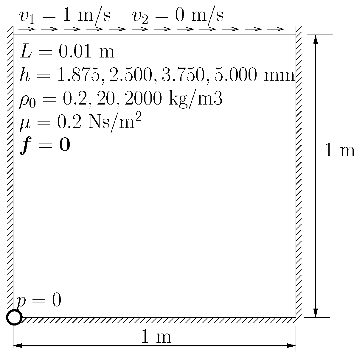
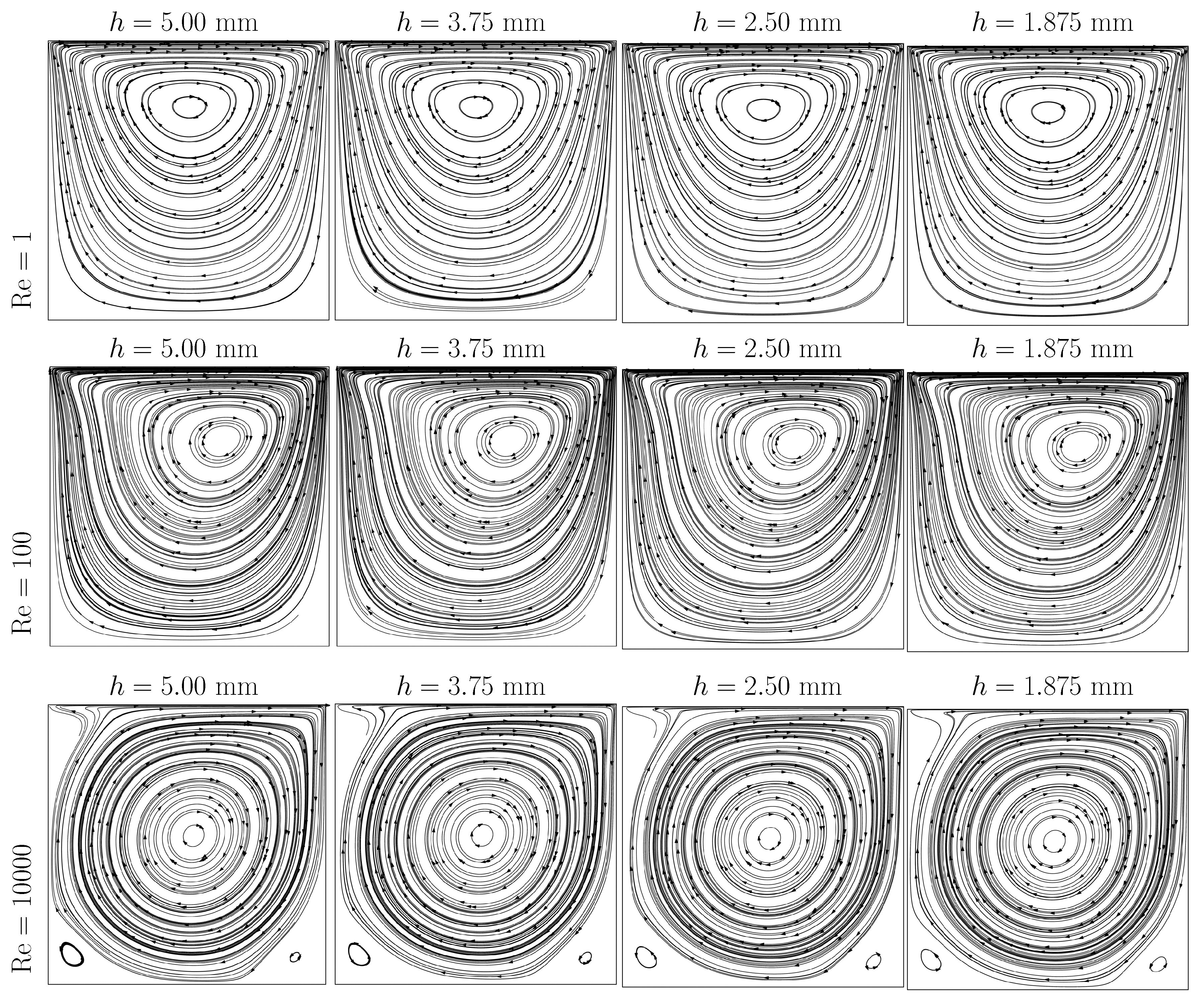
The solution of (49) makes use of the Newton method, with  a very intricate Jacobian. The specific source code is available in GitHub [32] as files turbulence.nb and turbulence.f90. For the driven cavity, see Figure 2; streamlines for the turbulent case are shown in Figure 3.
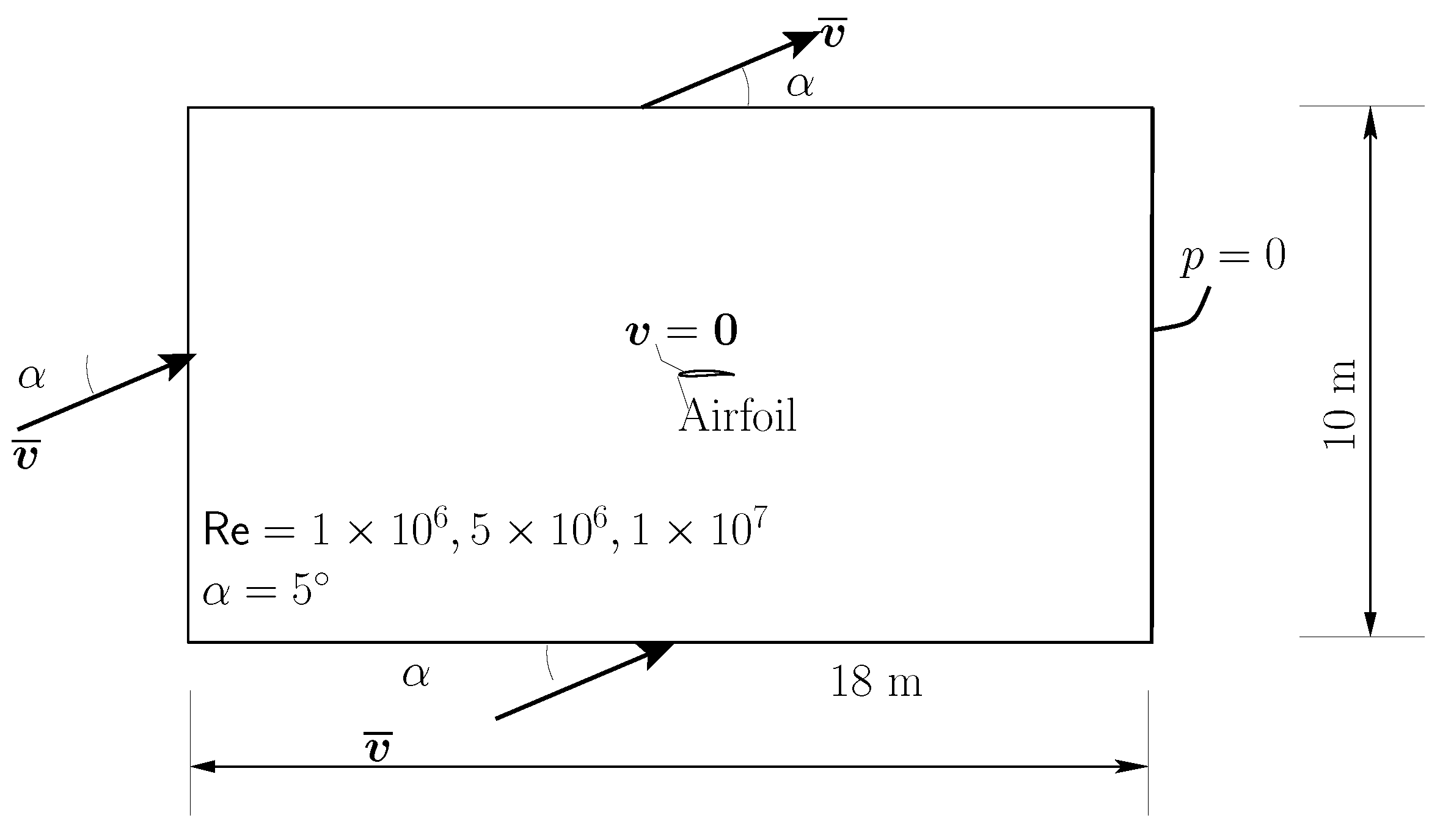
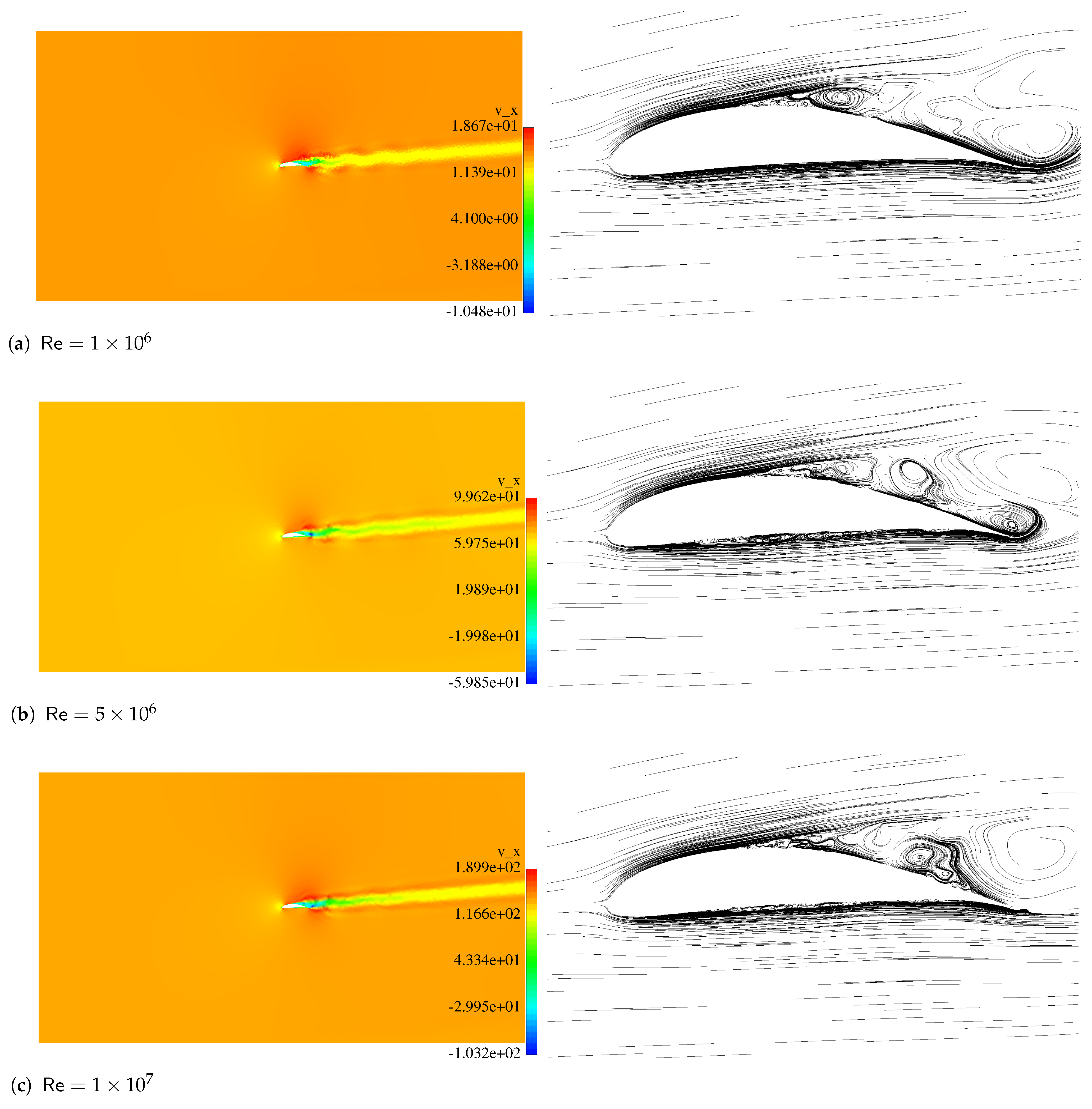
We adopted a control volume consisting of a rectangle, including the airfoil geometry, as shown in Figure 4. The chord line has a 1 m length. For  α = 5 and the optimized airfoil, we present the results in Figure 5 for the optimized airfoil. The velocity contour plots for the conditions are presented in Figure 4 along with the velocity lines in the neighborhood of the airfoils. A video of the optimized case flow for Re = 1 × 10 7 is available on the video repository [37].
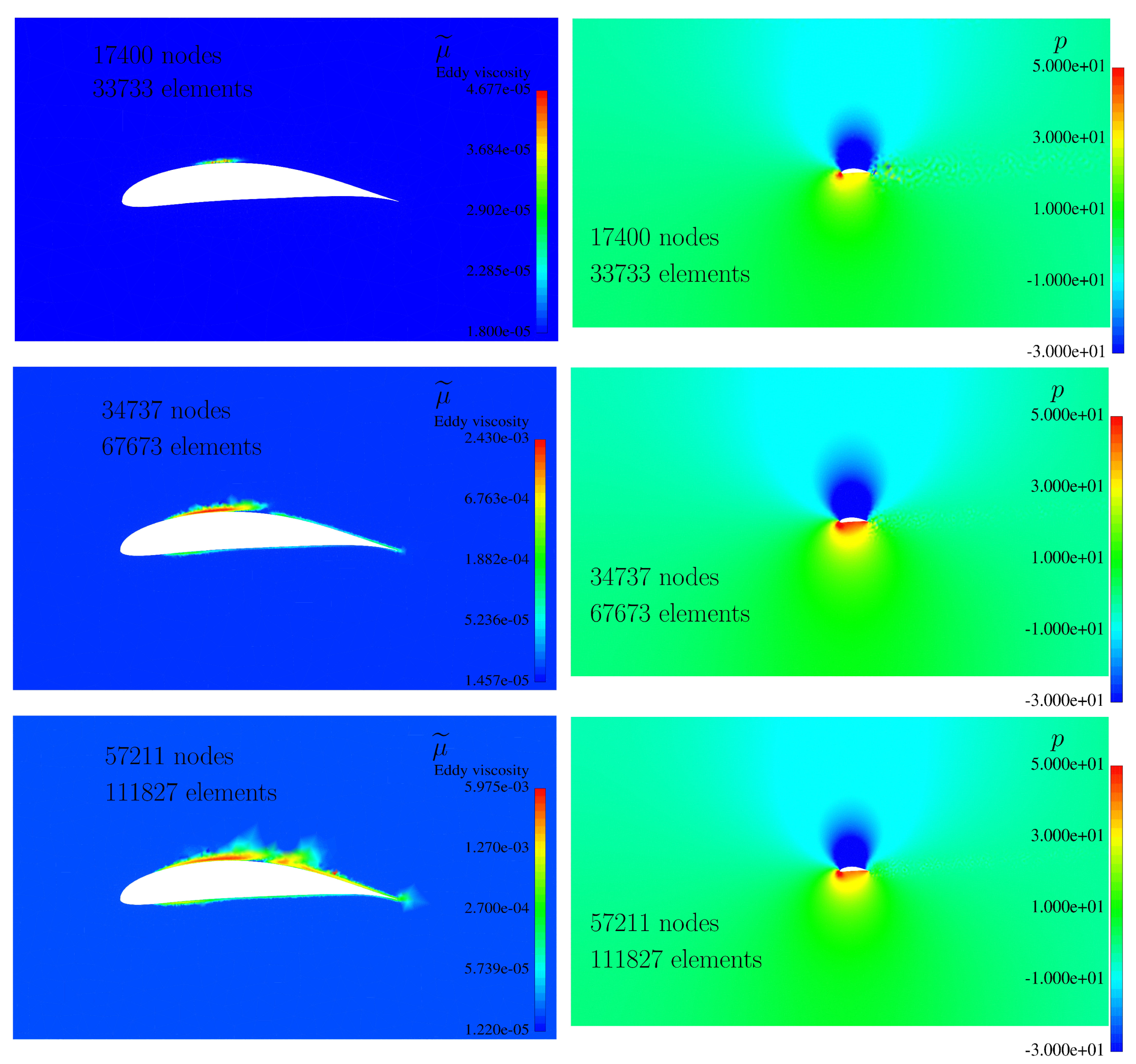
The convergence of results for the eddy viscosity μ ˜ and pressure p using three distinct meshes (17,400, 34,737, and 57,211 nodes) shows that smoothness increases with mesh refinement. Figure 6 shows the convergence of these fields.

5. Machine Learning and Optimization

The optimized airfoil optimization procedure consists of two stages: in the first stage, the relation between the CST parameters and the lift/drag ratio is established by machine learning. In the second stage, this function is maximized. In the first stage, we resort to the machine learning algorithm to actually construct a regression relating C L / C D with 10 parameters defining the upper and lower faces of the airfoil. The optimization processes in the second stage are based on the dual annealing algorithm. We make use of the libraries TensorFlow [38,39], SciPy, and NumPy. Optimization is performed with the function SciPy.optimize.dual_annealing. It uses a generalization of simulated annealing with a final gradient-based local search stage. C L / C D gradients are available from the machine learning model. In practice, the machine learning system makes use of a large set of input and output data, relates it statistically, and establishes the rules for regression. More data and better data will produce a better regression [39]. We note that, although possible (see, e.g., [10,40], the intent here is not to use full-feature machine learning to replicate the finite element simulations, but rather to extract the C L / C D ratio.
In summary, the machine learning algorithm involves three parts:
  • Parameter inputs, which are the 10 parameters of the CST representation for the complete set of UIUC airfoils.
  • Outputs, which are images under a function of the inputs, in this case, C L / C D .
  • Assessment method: this is required to measure the evolution of the iterations toward the result.
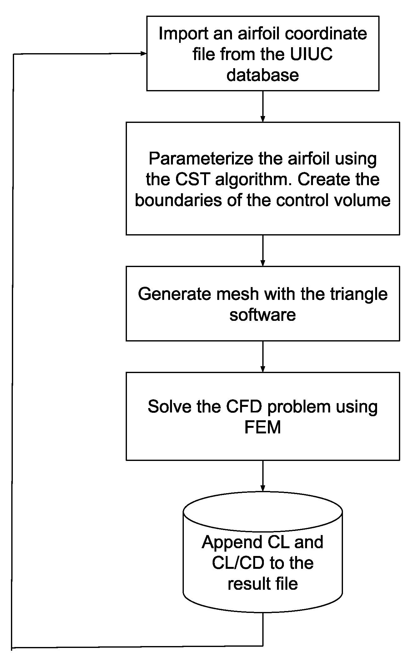
The data collection was performed with the flowchart in Figure 7. A total of 1598 airfoils from the UIUC database were considered valid for this application. Specific features of the machine learning procedure are as follows (see also [41]):
  • CST [22] parameterization with 10 parameters, which are both the inputs in the learning process and the design variables.
  • Data source: UIUC database [9].
  • Four angles of attack were tested, 0, 1.25, 2.50, and 5.00 degrees.
  • Set partitioning is as follows: 80% for training and 20% for testing.
  • The type is “Regression Classification”.
  • Activation function is “ReLU”.
  • Kernel initializer is a uniform distribution with HeUniform class.
  • Four dense layers.
  • 6000 epochs.
  • Loss function is “MAE”.
  • Adam optimizer for the stochastic gradient descent.
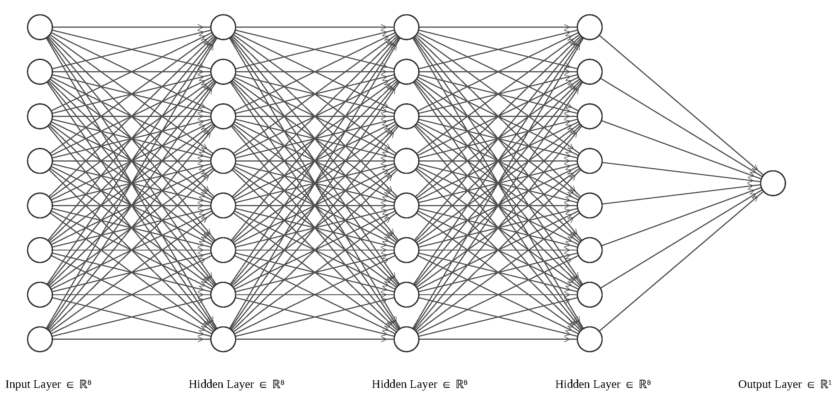
We make use of the deep learning framework, the Keras CNN dense neural network, which is adequate for regression. The network diagram is shown in Figure 8 for 8 inputs (omitting Δ ζ l and Δ ζ u ).
The reasons for these options are as follows. The UIUC database contains a total of 1621 airfoils but we found that 23 were unsuitable for parameterization by the CST algorithm. Since at least a single CST patch is needed for each surface, the minimum number of CST parameters is 10. Further increasing the number of parameters would create difficulties for the machine learning stage. The number and values of angles of attack are aligned with what is typical in recreational airplanes, ensuring that simulations preclude stalling. The type of procedure is “Regression Classification” since the purpose of simulation here is to be reproduced by the machine learning model. The “ReLU” activation function is adopted due to the vanishing gradient issue that occurred with other functions. Since an optimization algorithm (with a final gradient-based stage) is run on top of the machine learning model, this advantage is important. In addition, due to sparsity, good performance is achieved with the “ReLU” activation function. The layer and epoch numbers are the results of the experimentation.
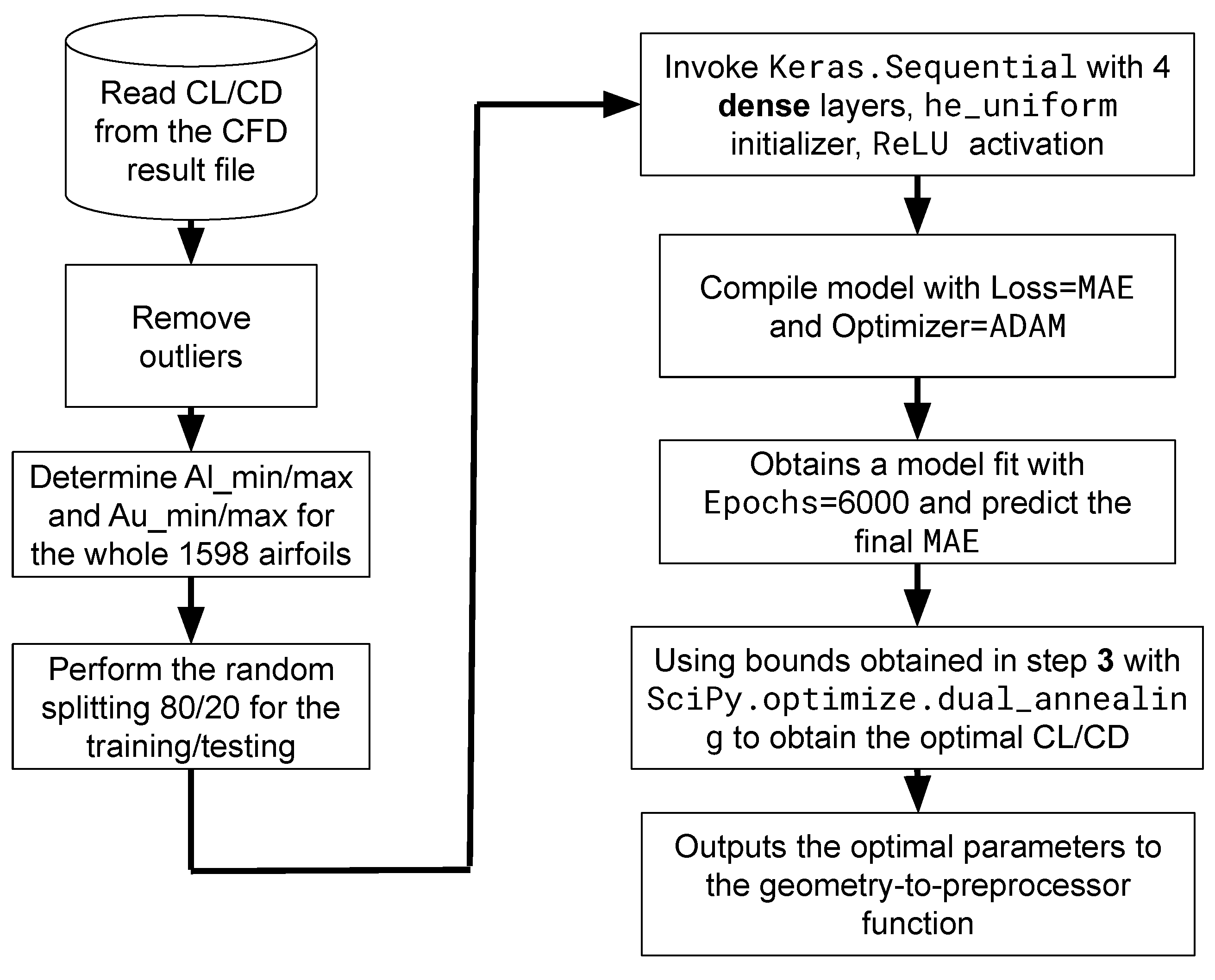
A flowchart for the algorithm following the data collection depicted in Figure 7 is shown in Figure 9.

6. Results and Discussion of Airfoil Optimization

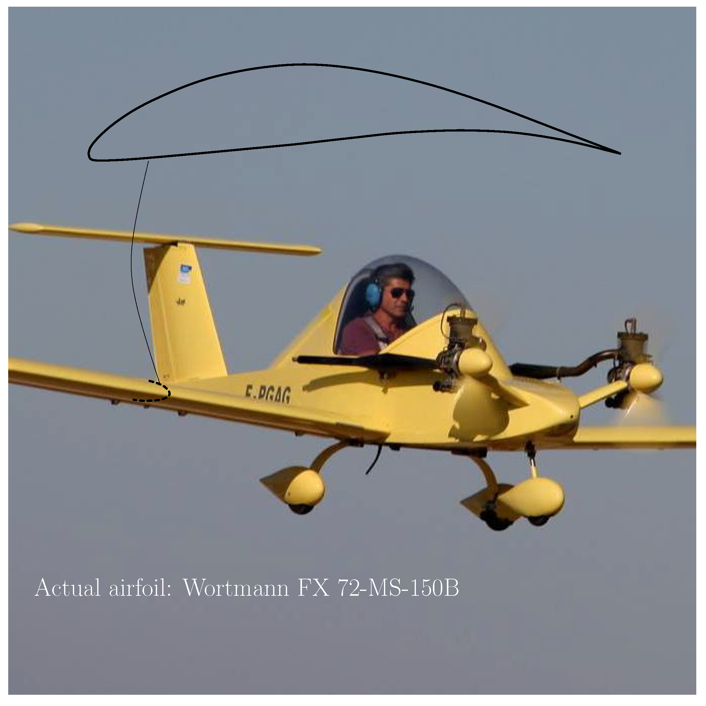
With a lightweight airplane, such as the MC12 Cri-Cri airplane shown in Figure 10, efficiency is paramount, even at the expense of lift. High values of C L / C D can be observed in recreational airplanes. By complying with this requirement, we are fulfilling two requirements, one is to maximize efficiency and the other is to avoid stalling. In this type of analysis, attention is focused on the behavior of the boundary layer, known as the layer of fluid close to a surface, a layer that strongly depends on the Reynolds number, the shape of the airfoil, and its inclination. Evaluating the boundary layer has the objective of reducing resistance measured by the resistance coefficient C D , composed of two effects, pressure resistance δ * and frictional resistance C L [42].
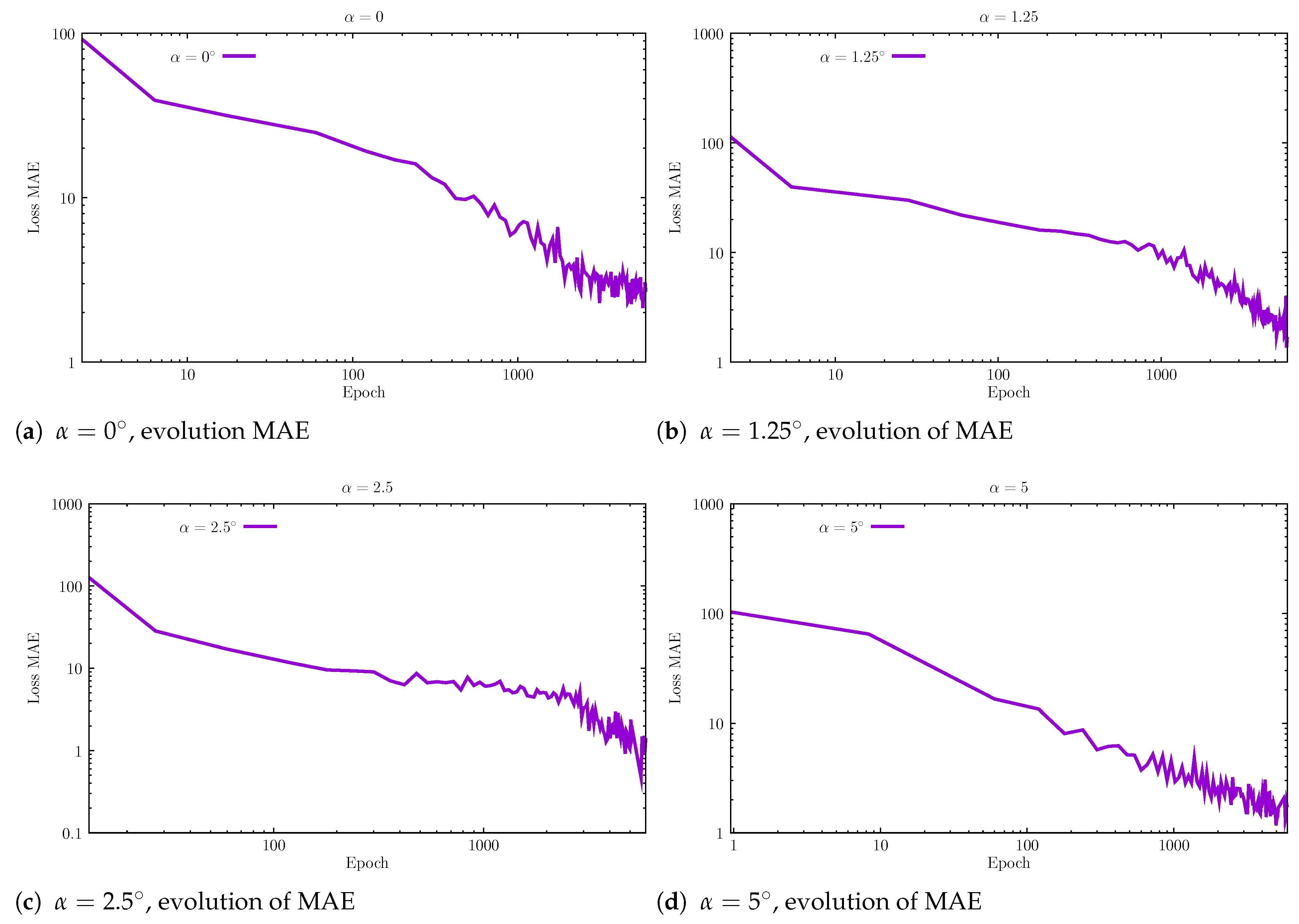
Using Keras/TensorFlow [38,39] combined with global optimization, it is possible to train and then optimize the value of C L / C D using (i) XFOIL [18] results or (ii) FEM RANS [19]. In terms of optimization, the toolkit from SciPy was adopted with the function optimize.dual_annealing. We show the evolution of loss and MAE (mean absolute error) in TensorFlow [38], as functions of the epochs, from which we have 6000, in Figure 11 for the four considered angles of attack: α = 0 , 1 . 25 , 2 . 50 and 5 . The precision is sufficient for obtaining airfoil profiles in parametric form, which are superior to those in the UIUC database [9].
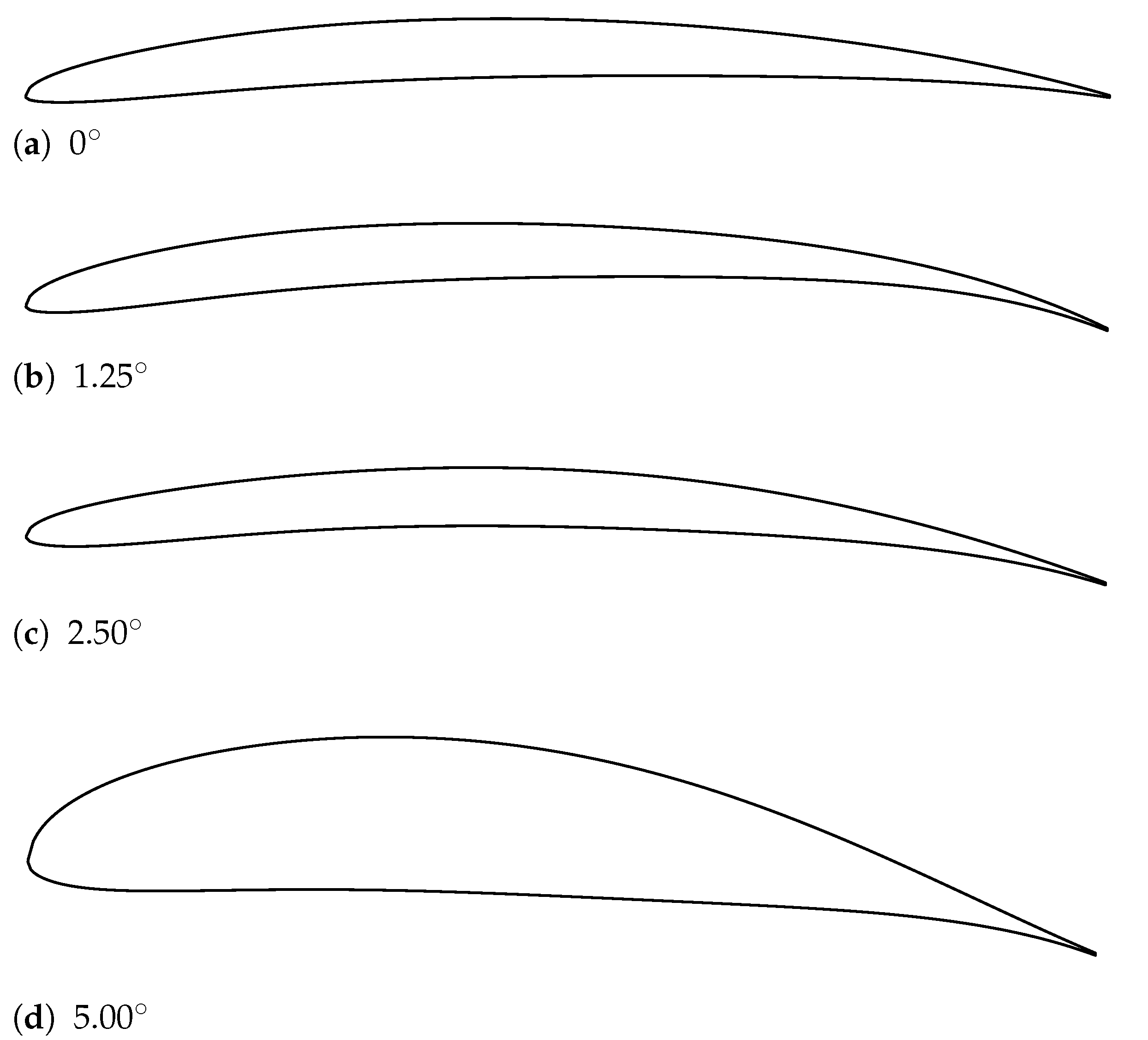
Optimized airfoils, each exhibiting positive curvature, are depicted in Figure 12. When analyzing the optimized airfoil for α = 0 , the positive curvature stands out. This configuration, despite being obtained for α = 0 , subjects the airfoil to higher pressure on the lower surface compared to the upper surface, producing a positive lift. There is a certain bounce on the leading edge, which, together with the curvature and its thickness, alter the behavior of the boundary layer, trying to keep it close to the airfoil, inhibiting separation. It should be noted that, as the angle of attack increases, the curvature tends to not be as pronounced; this happens due to the progressive increase in the contribution of the angle of attack to the increase in lift, leaving the airfoil to have such a pronounced curvature to compensate for this need. This observation is even clearer for the 5 case. It is known [42] that, at small angles of attack, thinner airfoils are preferable; at higher angles of attack, thicker airfoils are preferable. Comparing with the CST-parameterized versions of the UIUC database (pristine versions can be significantly different), both FEM and XFOIL show better C L / C D results, see Table 1, with similar performances for this target. In terms of C L alone, this table also shows that significant differences exist for very similar airfoils. Specific parameters are shown in Table 2 and can be tested in XFOIL by the reader.
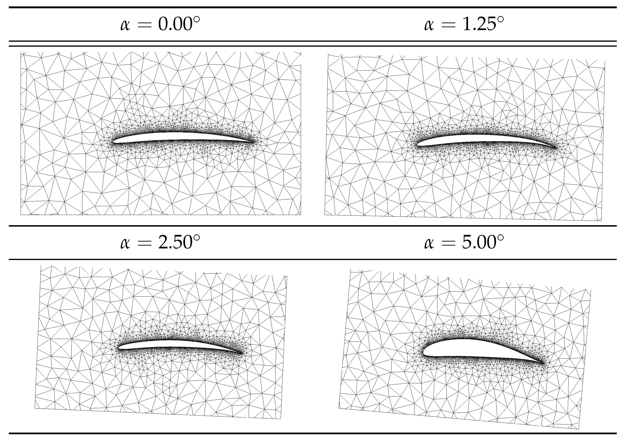
For the four optimal airfoils, we use SIMPLAS [19] with uniformly imposed velocity and initial conditions; v = 15 { cos α , sin α } . Meshes are refined locally, as shown in Figure 13.
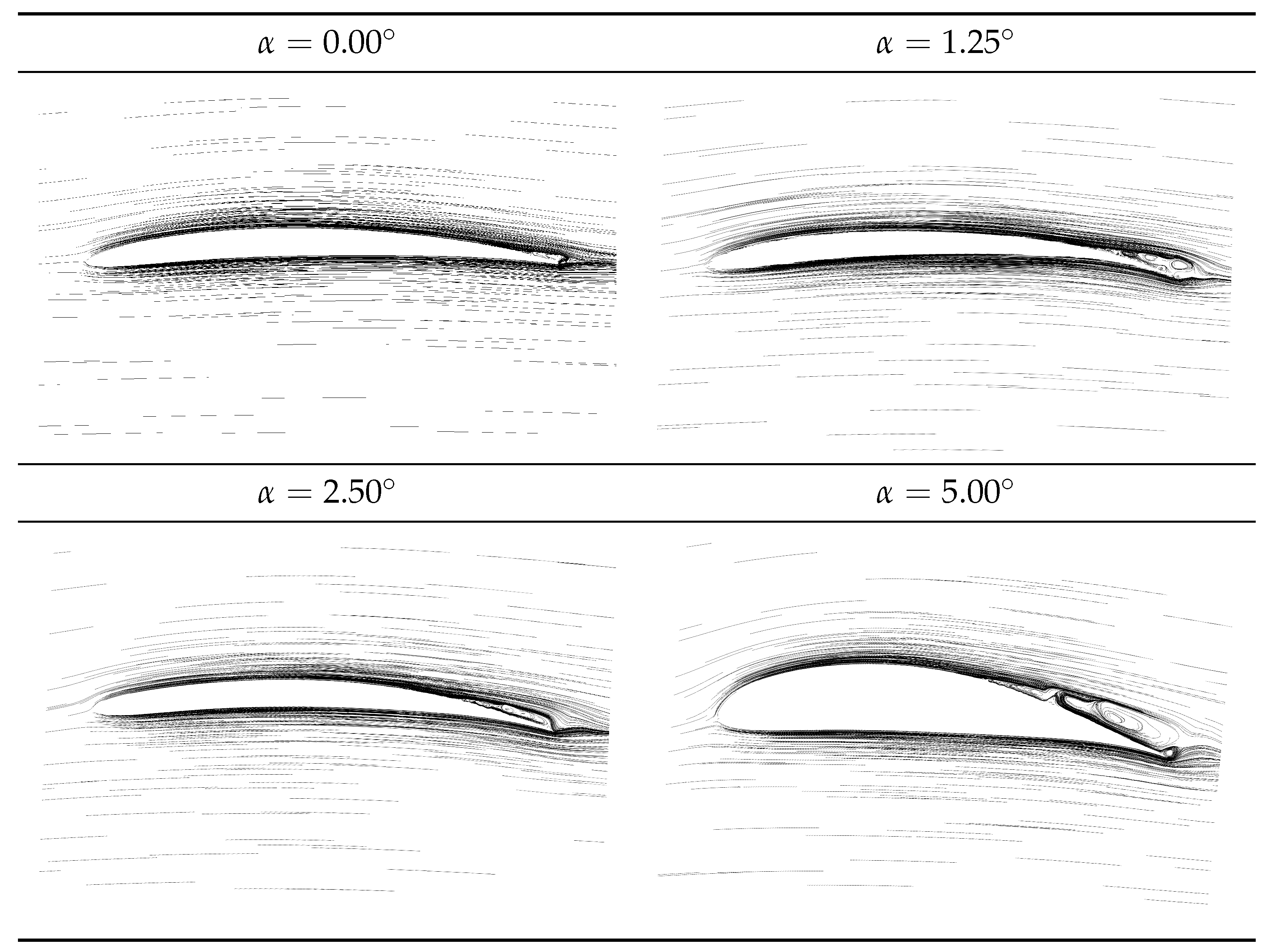
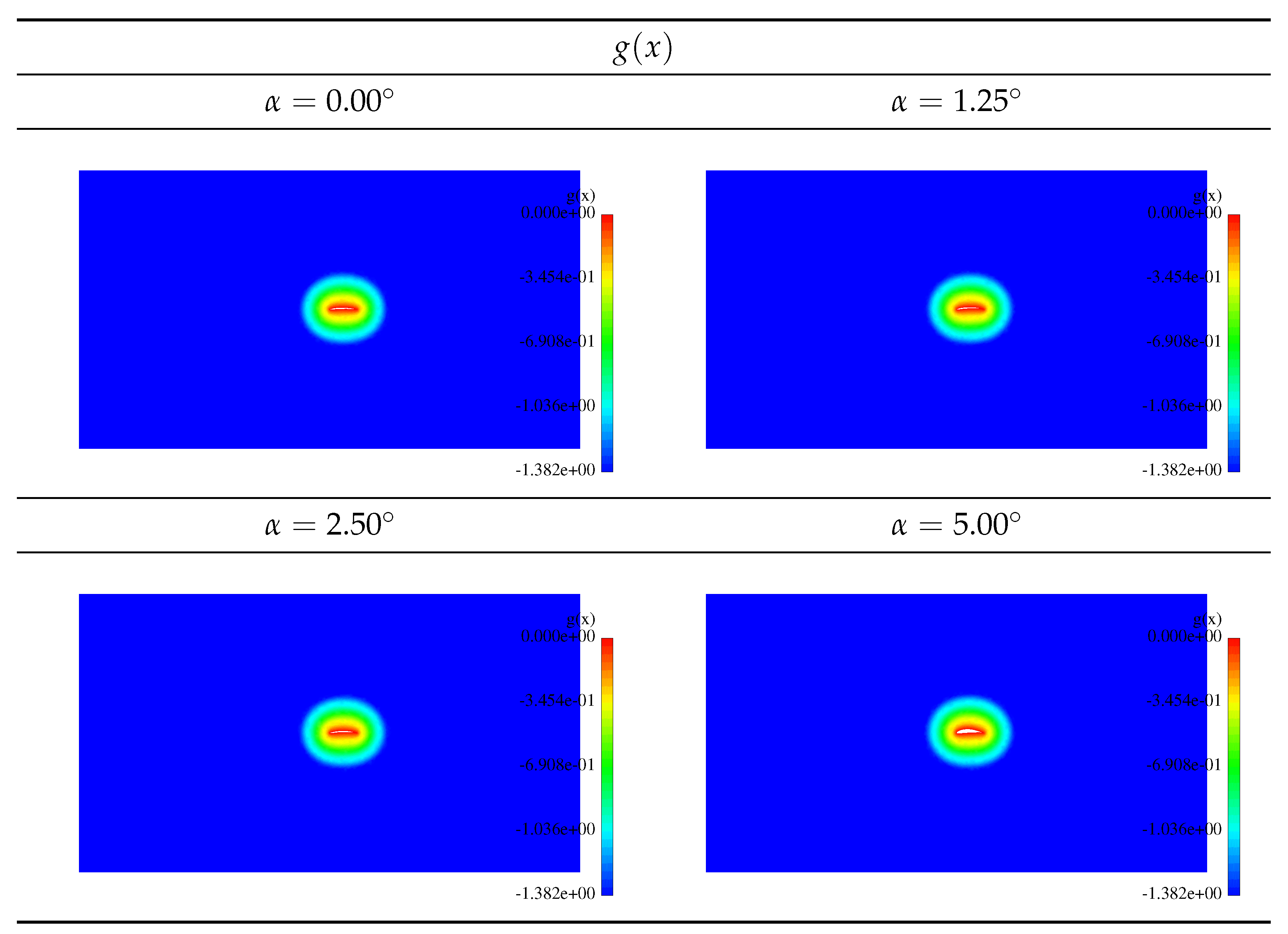
Velocity profiles for all four optimized airfoils resulting from the FEM analysis are shown in Figure 14. We can observe the aforementioned effects. For the ADF g ( x ) , Figure 15 shows the results.

7. Conclusions

From a representation point-of-view, specifically in the case of C L / C D , as well as in the shape optimization of airfoils, we achieved great success. An unconditionally stable, fully implicit time integrator was adopted. The use of Petrov–Galerkin finite elements (FE) for these applications presented no instabilities and the vortices were close to what was obtained in the finite volume analysis. The machine learning algorithm, which used 6000 epochs, was moderately successful, as not all CST versions of the airfoils in the UIUC database were reliable. Optimization produced better airfoils than those present in the UIUC database; these advancements were in line with the known details that are the rule of thumb within the recreational aircraft community.

Author Contributions

P.A.: Conceptualization, software, writing—original draft preparation; R.M.: methodology, and R.C.: investigation. All authors have read and agreed to the published version of the manuscript.

Funding

Thisresearch was funded by FCT, through IDMEC, under LAETA, project UIDB/50022/2020; FCT, through AEROG of the Laboratório Associado em Energia, Transportes e Aeronáutica (LAETA), under LAETA, project UIDB/50022/2020; UIDP/50022/2020, project LA/P/0079/2020.

Data Availability Statement

Not applicable.

Acknowledgments

Theairfoil data were made available by the University of Illinois Urbana-Champaign [9].

Conflicts of Interest

The authors declare no conflict of interest.

Abbreviations

The following abbreviations are used in this manuscript:
ADF  approximate distance function
CST  class function/shape function transformation
FEM  finite element method
MAE  mean absolute error
ML  machine learning
RANS  Reynolds-averaged Navier–Stokes equations

References

  1. Vanderplaats, G. Efficient algorithm for numerical airfoil optimization. J. Aircr. 1979, 16, 842–847. [Google Scholar] [CrossRef]
  2. Baydin, A.; Pearlmutter, B.; Radul, A.; Siskind, J. Automatic Differentiation in Machine Learning: A Survey. J. Mach. Learn. Res. 2018, 18, 1–43. [Google Scholar]
  3. Tao, J.; Sun, G. Application of deep learning based multi-fidelity surrogate model to robust aerodynamic design optimization. Aerosp. Sci. Technol. 2019, 92, 722–737. [Google Scholar] [CrossRef]
  4. Zanichelli, M. Shape Optimization of Airfoils by Machine Learning-Based Surrogate Models. Master’s Thesis, Politecnico Milano, Milan, Italy, 2021. [Google Scholar]
  5. Sun, Y.; Sengupta, U.; Juniper, M. Physics-informed deep learning for simultaneous surrogate modeling and PDE-constrained optimization of an airfoil geometry. Comput. Methods Appl. Mech. Eng. 2023, 411, 116042. [Google Scholar] [CrossRef]
  6. Wu, X.; Zuo, Z.; Ma, L. Aerodynamic data-driven surrogate-assisted teaching-learning-based optimization (TLBO) framework for constrained transonic airfoil and wing shape designs. Aerospace 2022, 9, 610. [Google Scholar] [CrossRef]
  7. Deng, F.; Yi, J. Fast inverse design of transonic airfoils by combining deep learning and efficient global optimization. Aerospace 2023, 10, 125. [Google Scholar] [CrossRef]
  8. Du, Q.; Liu, T.; Yang, L.; Li, L.; Zhang, D.; Xie, Y. Airfoil design and surrogate modeling for performance prediction based on deep learning method. Phys. Fluids 2022, 34, 015111. [Google Scholar] [CrossRef]
  9. Selig, M. UIUC Airfoil Data Site; Department of Aeronautica, Astronautical Engineering University of Illinois at Urbana-Champaign: Urbana, IL, USA, 1996. [Google Scholar]
  10. Hui, X.; Bai, J.; Wang, H.; Zhang, Y. Fast pressure distribution prediction of airfoils using deep learning. Aerosp. Sci. Technol. 2020, 105, 105949. [Google Scholar] [CrossRef]
  11. Karali, H.; Inalhan, G.; Demirezen, M.A. A new nonlinear lifting line method for aerodynamic analysis and deep learning modeling of small unmanned aerial vehicles. Int. J. Micro Air Veh. 2021, 13, 1–24. [Google Scholar] [CrossRef]
  12. Li, J.; Zhang, M.; Martins, J.; Shu, C. Efficient Aerodynamic Shape Optimization with Deep-Learning-Based Geometric Filtering. AIAA J. 2020, 58, 4243–4259. [Google Scholar] [CrossRef]
  13. Tyan, M.; Choi, C.K.; Ngyuyen, T.; Lee, J.W. Rapid airfoil inverse design method with a deep neural network and hyperparameter selection. Int. J. Aeronaut. Space Sci. 2023, 22, 33–46. [Google Scholar] [CrossRef]
  14. Xu, M.; Song, S.; Sun, X.; Chen, W.; Zhang, W. Machine learning for adjoint vector in aerodynamic shape optimization. Acta Mech. Sin. 2021, 37, 1416–1432. [Google Scholar] [CrossRef]
  15. Garcia-Gutierrez, A.; Gonzalo, J.; Dominguez, D.; Lopez, D.; Escapa, A. Aerodynamic optimization of propellers for high altitude pseudo-satellites. Aerosp. Sci. Technol. 2020, 96, 105562. [Google Scholar] [CrossRef]
  16. Rao, C.; Sun, H.; Liu, Y. Physics-informed deep learning for incompressible laminar flows. Theor. Appl. Mech. Lett. 2020, 10, 207–212. [Google Scholar] [CrossRef]
  17. Li, J.; Du, X.; Martins, J. Machine learning in aerodynamic shape optimization. Prog. Aerosp. Sci. 2022, 134, 100849. [Google Scholar] [CrossRef]
  18. Drela, M. XFOIL: An Analysis and Design System for Low Reynolds Number Airfoils. In Low Reynolds Number Aerodynamics; Mueller, T.J., Ed.; Springer: Berlin/Heidelberg, Germany, 1989; pp. 1–12. [Google Scholar]
  19. Areias, P. Simplas. Portuguese Software Association (ASSOFT) Registry Number 2281/D/17. Available online: http://www.simplassoftware.com (accessed on 20 June 2023).
  20. Shewchuk, J.R. Triangle: Engineering a 2D quality mesh generator and Delaunay triangulator. In Applied Computational Geometry towards Geometric Engineering; Lin, M.C., Manocha, D., Eds.; Springer: Berlin/Heidelberg, Germany, 1996; pp. 203–222. [Google Scholar]
  21. Anitha, D.; Shamili, G.; Ravi Kumar, P.; Sabari Vihar, R. Air foil shape optimization using CFD and parametrization methods. Mater. Today Proc. 2018, 5, 5364–5373. [Google Scholar] [CrossRef]
  22. Kulfan, B. Universal parametric geometry representation method. J. Aircr. 2008, 45, 142–159. [Google Scholar] [CrossRef]
  23. Lane, K.; Marshall, D. Inverse airfoil design using CST parameterization. In Proceedings of the Aerospace Sciences Meeting Including the New Horizons Forum and Aerospace Exposition, AIAA, Orlando, FL, USA, 4–7 January 2010. [Google Scholar]
  24. Gülçat, Ülgen. Fundamentals of Modern Unsteady Aerodynamics, 3rd ed.; Springer Nature: Cham, Switzerland, 2021. [Google Scholar]
  25. Research Inc. W. Mathematica. 2007. Available online: https://www.wolfram.com/mathematica/quick-revision-history/ (accessed on 20 June 2023).
  26. Korelc, J. Multi-language and multi-environment generation of nonlinear finite element codes. Eng. Comput. 2002, 18, 312–327. [Google Scholar] [CrossRef]
  27. Tezduyar, T.; Mittal, S.; Ray, S.; Shih, R. Incompressible flow computations with stabilized bilinear and linear equal-order-interpolation. Comput. Methods Appl. Mech. Eng. 1992, 95, 221–242. [Google Scholar] [CrossRef]
  28. Tezduyar, T.; Osawa, Y. Finite element stabilization parameters computed from element matrices and vectors. Comput. Methods Appl. Mech. Eng. 2000, 190, 411–430. [Google Scholar] [CrossRef]
  29. Tezduyar, T. Computation of moving boundaries and interfaces and stabilization parameters. Int. J. Numer. Methods Fluids 2003, 43, 555–575. [Google Scholar] [CrossRef]
  30. Tezduyar, T. Finite elements in fluids: Special methods and enhanced solution techniques. Comput. Fluids 2007, 36, 207–223. [Google Scholar] [CrossRef]
  31. Zienkiewicz, O.; Taylor, R.; Nithiarasu, P. The Finite Element Method for Fluid Dynamics; Elsevier: Waltham, MA, USA, 2014. [Google Scholar]
  32. Areias, P. Turbulent 2D Subroutines for SimPlas. 2023. Available online: https://github.com/PedroAreiasIST/Fluid (accessed on 20 June 2023).
  33. Varadhan, S. On the behavior of the fundamental solution of the heat equation with variable coefficients. Commun. Pure Appl. Math. 1967, 20, 431–455. [Google Scholar] [CrossRef]
  34. Spalart, P.; Allmaras, S. A one-equation turbulence model for aerodynamic flows. In Proceedings of the 30th Aerospace Sciences Meeting and Exhibit, Reno, NV, USA, 6–9 January 1992; American Institute of Aeronautics and Astronautics: Reston, VA, USA, 1992. [Google Scholar] [CrossRef]
  35. Spalart, P.; Allmaras, S. A one-equation turbulence model for aerodynamic flows. Rech. Aérospatiale 1994, 5–21. [Google Scholar] [CrossRef]
  36. NASA Langley Research Center. The Spalart-Allmaras Turbulence Model. Available online: https://turbmodels.larc.nasa.gov/spalart.html (accessed on 20 June 2023).
  37. Areias, P.; Melicio, R.; Correia, R. RANS with 10 Million Reynolds Number. 2015. Available online: https://youtu.be/W7_nEaoUn9k (accessed on 20 June 2023).
  38. Abadi, M.; Agarwal, A.; Barham, P.; Brevdo, E.; Chen, Z.; Citro, C.; Corrado, G.S.; Davis, A.; Dean, J.; Devin, M.; et al. TensorFlow: Large-Scale Machine Learning on Heterogeneous Systems. 2015. Software. Available online: TensorFlow.org (accessed on 20 June 2023).
  39. Mattmann, C. Machine Learning with TensorFlow, 2nd ed.; Manning: Shelter Island, NY, USA, 2020. [Google Scholar]
  40. Thuerey, N.; Weißenow, K.; Prantl, L.; Hu, X. Deep Learning Methods for Reynolds-Averaged Navier–Stokes Simulations of Airfoil Flows. AIAA J. 2020, 58, 25–36. [Google Scholar] [CrossRef] [Green Version]
  41. Chollet, F. Deep Learning with Python, 2nd ed.; Manning: Shelter Island, NY, USA, 2021. [Google Scholar]
  42. Brederode, V. Aerodinâmica Incompressível: Fundamentos, 2nd ed.; IST Press: Lisboa, Portugal, 2018. [Google Scholar]
Figure 1. Two-dimensional airfoil optimized using the CST parameterization.
Aerospace 10 00638 g001
Figure 2. Driven cavity: relevant data.
Aerospace 10 00638 g002
Figure 3. Driven cavity: streamlines for the turbulent case.
Aerospace 10 00638 g003
Figure 4. Control volume for the airfoil analysis.
Aerospace 10 00638 g004
Figure 5. Velocityin the x direction for Re = 1 × 10 6 , Re = 5 × 10 6 and Re = 1 × 10 7 with the optimized airfoil for α = 5 .
Aerospace 10 00638 g005
Figure 6. Convergenceof μ ˜ and p with mesh refinement.
Aerospace 10 00638 g006
Figure 7. Collecting the data for the machine learning algorithm.
Aerospace 10 00638 g007
Figure 8. Structure of the dense DNN used for airfoil optimization.
Aerospace 10 00638 g008
Figure 9. Machine learning algorithm after simulation and data collection represented in Figure 7.
Aerospace 10 00638 g009
Figure 10. Colomban MC12 Cri-Cri airplane. Airfoil Wortmann FX 72-MS-150B p = { 0.071566 , 0.064309 , 0.087768 , 0.37435 , 0.24168 , 0.53136 , 0.47846 , 0.37806 } .
Aerospace 10 00638 g010
Figure 11. Evolutionof MAE in TensorFlow for α = 0 , 1 . 25 , 2.5 and 5 .
Aerospace 10 00638 g011
Figure 12. Optimized airfoils as a function of α for Re = 1.08333 × 10 6 (our FEM analysis).
Aerospace 10 00638 g012
Figure 13. Locally refined meshes for the optimal FEM analysis of airfoils.
Aerospace 10 00638 g013
Figure 14. Steady state analysis: velocity profiles
Aerospace 10 00638 g014
Figure 15. Steady state analysis: g ( x ) .
Aerospace 10 00638 g015
Table 1. Optimized C L / C D and corresponding C L for the optimized airfoils.
(a) C L / C D for Re = 1.08333 × 10 6
Optimized
α XFOIL CST C L = FEM CST C L = Best-in-Database    C L =
0 160 160 105
1.25 223 222219
2.50 190 200 179
5.00 174 174 173
(b) C L for  Re = 1 . 08333 × 10 6
α XFOIL CSTFEM CST
0 0.98 0.61
1.25 1.12 1.08
2.50 0.93 1.04
5.00 1.49 1.49
Table 2. Optimal parameters for each α (8 out of 10, since two parameters are always close to zero for the UIUC database [9]).
Method α p
XFOIL0 { 0.06220 , + 0.17723 , + 0.01487 , + 0.35473 , + 0.13862 , + 0.26888 , + 0.21769 , + 0.48022 }
1.25 { 0.05168 , + 0.16828 , + 0.02512 , + 0.36842 , + 0.15012 , + 0.25799 , + 0.20649 , + 0.46556 }
2.50 { 0.06417 , + 0.12845 , + 0.04564 , + 0.23788 , + 0.11283 , + 0.19201 , + 0.27182 , + 0.33103 }
5.00 { 0.11054 , + 0.12032 , 0.07856 , + 0.26166 , + 0.29534 , + 0.37376 , + 0.49289 , + 0.31190 }
FEM0 { 0.03657 , + 0.09307 , + 0.01908 , + 0.14870 , + 0.11846 , + 0.20004 , + 0.19177 , + 0.28882 }
1.25 { 0.04173 , + 0.15715 , + 0.03088 , + 0.35488 , + 0.14013 , + 0.24550 , + 0.19497 , + 0.45997 }
2.50 { 0.05352 , + 0.13974 , + 0.03518 , + 0.25026 , + 0.12340 , + 0.19195 , + 0.28454 , + 0.31778 }
5.00 { 0.12164 , + 0.10912 , 0.06778 , + 0.26281 , + 0.30829 , + 0.36001 , + 0.49893 , + 0.32502 }
Disclaimer/Publisher’s Note: The statements, opinions and data contained in all publications are solely those of the individual author(s) and contributor(s) and not of MDPI and/or the editor(s). MDPI and/or the editor(s) disclaim responsibility for any injury to people or property resulting from any ideas, methods, instructions or products referred to in the content.