Article

JT9D Engine Thrust Estimation and Model Sensitivity Analysis Using Gradient Boosting Regression Method

1
Department of Aeronautical Engineering, Chaoyang University of Technology, Taichung 413, Taiwan
2
Department of Mechanical Engineering, Lungwa University of Science and Technology, Taoyuan 333, Taiwan
3
Aerospace Technology Research and Development Center, Taichung 433, Taiwan
*
Author to whom correspondence should be addressed.
Aerospace 2023, 10(7), 639; https://doi.org/10.3390/aerospace10070639
Submission received: 10 June 2023 / Revised: 9 July 2023 / Accepted: 14 July 2023 / Published: 15 July 2023
(This article belongs to the Special Issue Machine Learning for Aeronautics)

Abstract

:
In recent years, artificial intelligence (AI) technology has been applied in different research fields. In this study, the XGBoost regression model is proposed to estimate JT9D engine thrust. The model performance mean absolute error (MAE) is 0.004845, the mean-squared error (MSE) is 0.000161, and the coefficient of determination (R2) values of the training, validation, and testing subsets are 0.99, 0.99, and 0.98, respectively. Based on a model sensitivity analysis, the four parameters’ optimal values are as follows: the number of estimators is 900; the learning rate is 0.1; the maximum depth is 4, and the random state is 3. In addition, a comparison between the model performance in this study and that in a previous one was conducted. The MSE value is as low as 0.000021.

1. Introduction

The JT9D engine program was introduced in 1965 by Pratt and Whitney, who conducted the first engine test in 1966. Its advanced mechanical design technology and excellent turbofan engine performance were then exploited successfully in the military J58 turbofan engine [1]. In the 1970s and 1980s, the national aeronautics and space administration (NASA) implemented some technologies related to the JT9D turbofan engine. In 1978, two kinds of research were conducted on the JT9D engine in regard to its performance deterioration and the analytical study of the thermal barrier coating of the first-stage blades [2,3]. In 1980, the performance and deterioration of the CF6/JT9D engine were investigated by NASA [4]. Furthermore, NASA presented another report in 1982 investigating flight loads on the Boeing 747 aircraft, which used the JT9D turbofan engine [5]. Since the JT9D engine began to serve on the Boeing 747 aircraft in 1970, it has proven itself as the workhorse for the early 747, 767, A300, A310, and DC-10 aircraft models, with more than 3200 engines delivered in total [6].
An analysis of the JT9D engine’s power was conducted by Onal and Turan using aero-engine momentum and continuity equations [7]. Fang et al. successfully built the FMI-based multidomain simulation of the JT9D engine control system [8]. The estimation of engine thrust is the primary objective of an engine control system. Therefore, Maggiore et al. proposed an estimator design to handle the nonlinear dynamics system of a jet engine [9]. Zhou and Zhang presented a study report on engine thrust estimation using an ensemble of improved wavelet extreme learning machines to satisfy the conditions of direct thrust control [10]. In addition, Oruc and Bakircioglu used a particle swarm optimization algorithm to model JT9D engine thrust; in this study, the investigators found high-accuracy thrust values during cruise flights [11]. A study was proposed to investigate the application of artificial neural networks in accurately predicting aircraft thrust by leveraging the capability of ANNs to learn from large datasets [12].
In recent years, artificial intelligence (AI) technology has been applied in different research fields, such as the prediction of the composition of syngas [13], the emissions of diesel engines [14], and aeroengine thrust estimations [15,16]. Furthermore, the XGBoost algorithm has been widely utilized for detection, disease diagnosis, classification, and predictions [17,18,19,20,21,22,23]. Based on the excellent performances of the XGBoost algorithm in previous research, the XGBoost regression model is proposed in the present study to estimate JT9D engine thrust. Nguyen-Sy et al. studied the XGB model to predict the compressive strength of concrete and perform a sensitivity analysis of the model parameters’ effects [23]. Sensitivity analysis was also applied to this study’s XGBoost model to investigate the effects of the parameters.

2. Materials and Methods

2.1. GT9D Turbofan Engine

In the research conducted by Jackson et al., the authors presented the performance and advanced design of the JT9D turbofan engine [1]. The specifications of the JT9D turbofan engine are listed in 
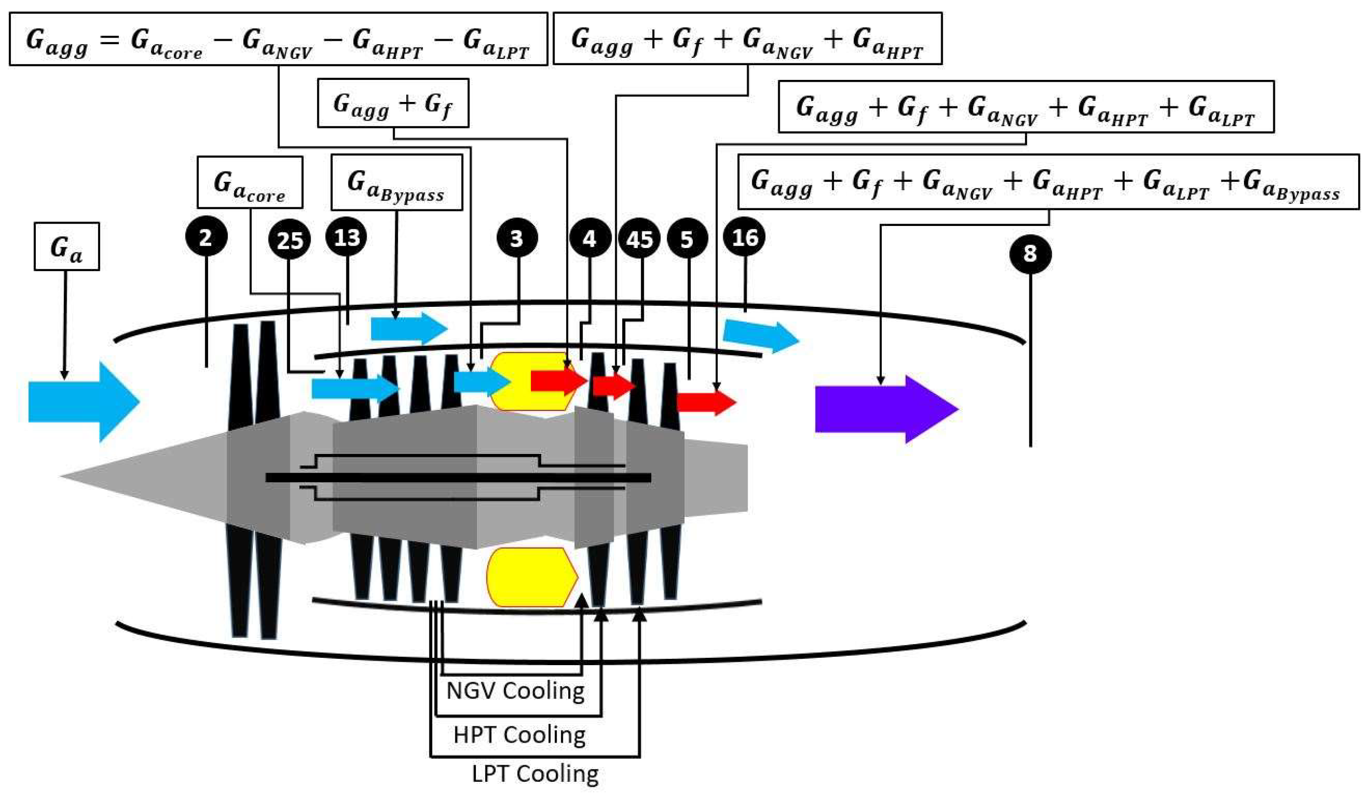
Table 1. The engine stations are as follows: Air flows through the inlet and enters the fan situated in station 2. The exit station of the fan is named 2.5. The bypass airs flow from stations 13 to 16. The exit for the compressor is at station 3, and the exit of the burner is at station 4. The compression process between stations 2.5 and 3 is meant to compress the air to achieve a pressure ratio according to the needs of the burner. The hot, high-pressure gas discharged from the burner (station 4) enters the high-pressure turbine that is connected to the compressor through a shaft. Then, the hot gas enters the low-pressure turbine in station 4.5 and exits the engine at station 5 [24]. Finally, the exhaust gas discharges from the nozzle name station 8. The schematic of the JT9D turbofan engine is shown in Figure 1.

JT9D Turbofan Engine Parametric Cycle Analysis

Parametric cycle analysis, which is a design point of the engine, studies the thermodynamic changes in the working fluid flowing through the engine [25]. NASA uses the numerical propulsion system simulation code to implement the thermodynamic performance analysis of aircraft gas turbine engine cycles [26]. The main focus of this analysis involves the operating characteristics of each module according to the principles of thermodynamics and turbomachinery; these are introduced as follows:
  • Fan
For a given fan pressure ratio ( π f ) and isentropic efficiency ( η f ) , the relationship between the fan total temperature and total pressure is as follows:
P t 25 = P t 2 π f
T t 25 = T t 2 1 + 1 η f π f γ a 1 γ a 1
where P t 25 is the total pressure at the outlet of the fan, T t 25 is the total temperature at the outlet of the fan, and γ a is the ratio of the specific heat of the cold airflow.
Because the air is compressed by the fan and guided into the bypass channel according to the set ratio, mixed with the core airflow at the outlet of the turbine, and then discharged from the nozzle to generate thrust, the ratio of the bypass airflow to the core airflow is defined as the bypass ratio, as follows:
R B y p a s s = G a B y p a s s G a c o r e
where R B y p a s s is the bypass ratio, G a B y p a s s is the bypass airflow, and G a c o r e is the core airflow.
2.
Compressor
The primary function of the compressor module is to compress the core airflow entering the engine and to provide combustion in the combustion chamber. The compressor pressure ratio is equal to LPC-Pt times HPC-Pt. When the pressure ratio is given, the total pressure of the outlet airflow can be calculated as follows:
P t 3 = π C P t 25
where P t 3 is the total pressure of the outlet airflow of compressor and π C is the compressor pressure ratio.
Then, according to the overall adiabatic compressor efficiency, η C = w C i d e a l w C a c t u a l = Δ h t C Δ h t C , the axial work required for the airflow to be compressed in the compressor can be calculated as follows:
W C = C p a T t 25 η C P t 3 P t 25 r a 1 r a 1
T t 3 = W C C p a + T t 25  
where W C is the compressor’s required work, C p a is the specific heat of the cold airflow, and T t 3 is the total temperature of the outlet airflow of the compressor.
To prevent the turbine blades from being burned due to high temperature, the compressor usually extracts part of the relatively low-temperature compressed air into the turbine; thus, the airflow entering the combustion chamber should be calculated as follows:
G a g g = G a c o r e G a N G V G a H P T G a L P T  
In Equation (7), G a N G V , G a H P T , and G a L P T represent the cooling airflow required to be extracted by the first-stage nozzle of the turbine, the high-pressure turbine, and the low-pressure turbine, respectively. Suppose the compressor is an n-stage axial flow compressor, and the cooling airflow is extracted from the outlet of the a-stage compressor. In this case, the pressure ratio of the cooling airflow can be calculated as follows:
π C o o l = π C n a
where π C o o l is the pressure ratio of the cooling airflow.
3.
Combustor
The primary function of the combustion chamber module is to provide a mixture of fuel and high-pressure gas for combustion to release the chemical energy for power, thereby increasing the temperature and thermal energy of the working airflow. The ideal combustion state in the combustion chamber should be equal-pressure combustion; however, in real conditions, pressure losses may be caused by friction and other factors. By defining the total pressure loss percentage Δ P , the total pressure of the airflow at the exit of the combustion chamber can be calculated as follows:
P t 4 = 1 Δ P P t 3
where P t 4 is the total pressure of the airflow at the exit of the combustion chamber, and Δ P is the total pressure loss percentage:
T t 4 = G f H V η B + C P a T t 3 G f + G a c o r e C P g G f + G a c o r e + T t 3
where T t 4 is the total temperature of the airflow at the exit of the combustion chamber, G f is the fuel flow, H V is the heating value, η B is the combustion efficiency, and C P g is the specific heat of the hot airflow.
4.
High-pressure turbine
The primary function of the high-pressure turbine is to convert the outlet airflow of the combustion chamber to shaft work in order to drive the rotation of the compressor. If a small part of the shaft work must be transferred for other purposes (i.e., power takeoff) owing to task requirements, such as driving the accessory gearbox, the shaft power extraction percentage is defined as P T O ; for the P T O , the principle of shaft power matching between the compressor and high-pressure turbine must be satisfied. Assuming that the mechanical efficiency η m e c h of the transmission between the compressor and high-pressure turbine is known, the high-pressure shaft work provided by the turbine can be calculated as follows:
W ˙ H P T = W ˙ C 1 P T O η m e c h
where W ˙ H P T is the high-pressure turbine shaft power, P T O is the shaft power extraction percentage, and η m e c h is the mechanical efficiency of the drive shaft between the high-pressure turbine and compressor.
Furthermore, according to the definition of the high-pressure turbine output shaft work,
W ˙ H P T = G a g g + G a N G V + G ˙ a H P T + G ˙ f × C P g T t 4 C P g T t 45
where T t 45 is the total temperature of the high-pressure turbine.
The total temperature of the airflow at the outlet of the high-pressure turbine can then be calculated as follows:
T t 45 = C P g T t 4 W ˙ H P T G ˙ a g g + G a N G V + G ˙ a H P T + G ˙ f C P g
Assuming that the airflow through the high-pressure turbine follows an adiabatic expansion process, its adiabatic efficiency η H P T can be defined as follows:
η H P T = h t H P T h t H P T = C P g ( T t 4 T t 45 ) C P g ( T t 4 T t 45 )
where h t H P T is the actual enthalpy for the high-pressure turbine, h t H P T is the ideal enthalpy for the high-pressure turbine, and T t 45 is the total temperature of the ideal high-pressure turbine.
The total temperature of the outlet airflow of the high-pressure turbine in the ideal process can be deduced through the transposition of Equation (11), as follows:
T t 45 = T t 4 T t 4 T t 45 η H P T
The total pressure at the outlet airflow of the high-pressure turbine can then be deduced according to the isentropic relationship, as follows:
P t 45 = P t 4 T t 45 T t 4 γ γ 1
where P t 45 is the total pressure of the high-pressure turbine.
5.
Low-pressure turbine
The primary function of the low-pressure turbine is the conversion of the heat energy of the airflow introduced from the high-pressure turbine to shaft power for driving the rotation of the fan. The calculations for the changes in airflow properties are similar to those of the high-pressure turbine, because the shaft work must be matched between the fan and low-pressure turbine (according to the power-matching principle). Hence, on the premise that the mechanical efficiency of the shaft work transfer between the two modules is known, the formula for the shaft work output per unit time of the low-pressure turbine can be deduced as follows:
W ˙ L P T = W ˙ F η m e c h
where W ˙ L P T is the low-pressure turbine shaft power.
Then, the low-pressure turbine output shaft work per unit time can be defined as follows:
W ˙ L P T = ( G ˙ a g g + G ˙ a N G V + G ˙ a H P T   + G ˙ a L P T + G ˙ f ) C P g T t 45 T t 5
where T t 5 is the total temperature of the low-pressure turbine.
The total temperature of the airflow at the outlet of the low-pressure turbine is then calculated as follows:
T t 5 = T t 45 W L P T C P g ( G ˙ a g g + G ˙ a N G V + G ˙ a H P T   + G ˙ a L P T + G ˙ f )
Suppose that the airflow passing through the low-pressure turbine is assumed to be an adiabatic expansion process. Thus, its adiabatic efficiency η L P T can be defined as follows:
η L P T = h L P T h L P T = C P g ( T t 45 T t 5 ) C P g ( T t 45 T t 5 ) = T t 45 T t 5 T t 45 T t 5
where h t L P T is the actual enthalpy for the low-pressure turbine, h t L P T is the ideal enthalpy for the low-pressure turbine, and T t 5 is the total temperature of the ideal low-pressure turbine.
From Equation (20), the total temperature of the outlet airflow of the low-pressure turbine in the ideal process can be deduced as follows:
T t 5 = T t 45 T t 45 T t 5 η L P T
The total pressure of the outlet airflow of the low-pressure turbine can then be deduced according to the isentropic relationship, as follows:
P t 5 = P t 45 T t 5 T t 45 γ γ 1
where P t 5 is the total pressure of the low-pressure turbine.

2.2. GT9D Turbofan Engine Data

Simulations are used to collect the dataset at the component level of the JT9D turbofan engine [27]. The 13 features selected for the AI model are listed in Table 2. A total of 12 features were chosen for the AI model inputs, including the fuel flowrate (Wf), combustion chamber exit temperature (T4), and nozzle exit temperature (T8). The engine thrust (Fg) is the expected target value of the AI model. The selection of the 12 input features selection was based on the research of Wang et al. [16]. Furthermore, the thrust simulation results of Wang and this study could be compared to evaluate the accuracy.

JT9D Turbofan Engine Data

The total number of samples obtained in the data collection was 438. Figure 2a shows the violin plots depicting the summary statistics and densities of HPS-Nmech and Fg. The broader areas of the violin plots represent higher probabilities that the members of the population will take on the given values; conversely, the narrower areas represent lower probabilities. For instance, in Figure 2a, the white dot represents the median and the black bar in the center represents the interquartile range. The top of the black bar represents the third quartile, and the bottom represents the first quartile. Figure 2b–d shows the summary statistics and densities of T4, LPS-Nmech, T45, T8, P4, P45, Wfuel, HPC_Pt, LPC_Pt, HPT_Pt, and LPT_Pt. The exact interquartile range values are listed in Table 3.
The statistical analysis results between the model input features and target are represented visually in Figure 3. From Figure 3, it can be observed that parts of the input features are proportional to the engine thrust Fg, such as Wfuel, P4, T4, HPS_Nmech, P45, and T8. Figure 3a shows the results of the thrust increasing due to the increase in the fuel flow rate. This means that energy sustainably increases when more fuels are sprayed into the combustion chamber. Furthermore, Figure 3d shows that the pressure loss in the combustion chamber affects the thrust. The most important factor affecting the thrust is the temperature exit from the combustion chamber, shown in Figure 3e. A higher T4 value means that a higher thrust can be created. This is a similar effect to that of the aforementioned fuel flow rate. It is noted that even at the same temperature values, the thrust also increases because the cooling consideration limits the temperature value in the case of burnout. The relationships between the other input features and Fg also show proportional trends but are limited by the power matching and cooling considerations.

2.3. XGBoost Model

Chen and Guestrin proposed a novel sparsity-aware algorithm, which is an open-source package for approximate tree learning called the XGBoost. The XGBoost algorithm can effectively reduce calculation costs while providing a higher model performance [28]. Figure 4 shows the flowchart of the proposed XGBoost algorithm model for engine thrust prediction. In the research of Wang et al., the percentages of splitting the dataset for different combinations were investigated [16]. There are three ratios for the training and testing datasets: 8:2, 6:4, and 5:5. The ratio 8:2 had the lowest MSE value, which indicated an excellent model performance. In the present study, the dataset was split into three subsets using the Python sklearn library train_test_split code, so that 70% was used for model training needs, 10% was used for the validation of the model’s performance, and the remaining 20% was used for model testing. The primary parameters of the XGBoost model are as follows: for the Max_depth, denoting the maximum depth of the tree, the default value is 6; this was set to 4 in this study to prevent overfitting. N_estimators represents the number of trees used for boosting, whose value was set to 900 herein. The Learning_rate indicates the learning rate that determines the step size at each iteration while reaching a minimum loss function; the lower the value of this parameter is, the better the performance is. Thus, this value was set to 0.1 in this study. Colsample_bytree denotes a family of parameters for subsampling the columns within the range of 0 to 1, and this value was set to 0.8. The subsample represents the training sample’s subsample ratio, which was set to 0.5. The parameter values of Colsample_bytree and the subsample ratio were determined using typical values based on experience.
The model’s performance reveals its accuracy, and the mean absolute error ( M A E ), mean-squared error ( M S E ), and coefficient of determination ( R 2 ) are the metrics used in this study to evaluate the model’s performance. The statistical equations for these metrics are as given in Equations (23)–(25), where P i is the predicted value obtained from the model and T i is the target value obtained from the dataset. P ¯ i is the average of the predicted values for the entire dataset.
M A E = 1 n i = 1 n T i P i
M S E = 1 n i = 1 n T i P i 2
R 2 = 1 i = 1 n P i T i 2 i = 1 n P ¯ i T i 2

3. Results

3.1. Model Performance

The model performances are listed in Table 4. These results were calculated based on Equations (20)–(22). According to Equation (22), if the predicted values are close to the target values, the R2 value approaches 1. The M A E and M S E values are calculated based on the min–max normalization values of the dataset. In this model, the R 2 value is 0.99, which means that the predicted values are relative to the target values. Only the R2 value for the 20% dataset for testing is 0.98. This is unsurprising, because the testing dataset is used to test the model, and it is possible to obtain a lower R 2 value for the actual model. It also shows the outstanding performance of the XGBoost regression model. The scatter plot of the engine thrust predictions versus the dataset values is shown in Figure 5.

3.2. Sensitivity Analysis

3.2.1. Effect of the Number of Estimators

In the XGBoost model, the estimators represent the number of trees used for boosting. The range varies from 50 to 1100. The MSE and R2 values were observed during the estimator variation in the model training and testing. Figure 6a,b illustrate the MSE values for the model training and testing, respectively. Figure 6c,d represent the R2 values for the model training and testing, respectively. The opposite result is observed between the MSE and R2 values because of their definitions. While the number of estimators reaches 300, the lowest value of the MSE and the highest value of R2 were obtained for the training dataset, as shown in Figure 6a,c. The same trends were observed in Figure 6b,d, except for the lower value compared with the results in Figure 6a,c. The reason for this is that the model testing dataset was selected for testing only. Therefore, the model’s performance for the testing dataset was lower than that for the training dataset.

3.2.2. Effect of the Learning Rate

The learning rate determines the step size at each iteration while reaching a minimum loss function. The range varies from 0.04 to 0.4. The MSE and R2 values were also observed during the model training and the testing learning rate variation. Figure 7a,b illustrates the MSE values for the model’s training and testing, respectively. Figure 7c,d represents the R2 values for the model’s training and testing, respectively. While the learning rate reached 0.1, the testing dataset’s MSE had the lowest value, and the R2 value was the highest. These results determine the whole model’s performance.

3.2.3. Effect of the Max_depth

Max depth denotes the maximum depth of the tree. The range varies from 1 to 7. The MSE and R2 values were also observed during the model’s training and testing with max depth variation. Figure 8a,b illustrates the MSE values for the model’s training and testing, respectively. Figure 8c,d represents the R2 values for the model’s training and testing, respectively. While the max depth reached 4, the testing dataset’s MSE was the lowest, and the R2 value was the highest. These results show a similar trend to that of the learning rate sensitivity analysis.

3.2.4. Effect of the Random State

The random state value for splitting the train and test datasets was also investigated, because it controls the shuffling applied to the data before using the split. The random state value will directly determine the samples of the training, validating, and testing datasets and affect the model’s performance. The range varies from 1 to 7. The MSE and R2 values were also observed during the model’s training and testing with max depth variation. Figure 9a,b illustrates the MSE values for the model’s training and testing, respectively. Figure 9c,d represents the R2 values for the model’s training and testing, respectively. While the random state value reached 3, the testing dataset’s MSE was the lowest, and the R2 value was the highest. These results show a similar trend to that of the max depth sensitivity analysis.

4. Discussion

The deviations in the values between the validation dataset and its predictions are shown in Figure 10. The pink triangles and the blue squares stand for the validation dataset and the prediction of the validation dataset, respectively. Most predictions are close to the original validation dataset, reflecting the model’s outstanding performance. The deviations between the test dataset and its predicted values are shown in Figure 11. Most predictions are close to the original test dataset, especially when the engine thrust values are around 10,000 lbs; however, the deviations are more significant when the engine thrust values are over 30,000 lbs. These deviation numbers are obviously attributable to the fact that test dataset represents only 20% of the total dataset. Because the 20% testing dataset is for testing only, it is reasonable to infer that decreasing the testing dataset percentage would lead to a higher model performance, because the training dataset percentage would increase. Furthermore, Table 3 shows that the third quartile of the thrust dataset is 22,097.65 lbs. This statistic also reveals higher deviations between the actual and predicted thrust after the XGBoost regression model simulation, where the real thrust values are over 30,000 lbs.
Furthermore, the XGBoost regression model performance was validated by comparisons with the results reported by Wang et al. [16]. The MSE value in the present study is less than that of Wang’s model listed in Table 5, which indicates outstanding model performance.
The XGBoost regression model’s performance was investigated through model parameters such as the number of estimators, learning rate, max depth, and random state. These former three parameters directly relate to the model’s training and testing results and determine the final model performance. The last one is associated with the dataset split. The sample qualities of the dataset will also affect the model’s performance. Model sensitivity analyses were investigated by adjusting the range of these model parameters. These results are helpful in fully understanding the model’s training and testing processes. This procedure also helps the researcher to tune the model parameters. Based on the sensitivity analysis, the optimal parameters of the XGBoost model are listed in Table 6.

5. Conclusions

In this study, the statistical analysis of the violin plot and correlation between the input feature and target (thrust) of the JT9D engine data were calculated and plotted first. It is helpful to analyze and visualize the original data patterns and trends and to preprocess the dataset for model training.
Then, the thrust estimation model for the JT9D turbofan engine was successfully built based on the XGBoost regression model. The R2 values of the training, validation, and testing subsets were 0.99, 0.99, and 0.98, respectively. In addition, a comparison between the model performance in this study and that in a previous one was conducted. The MSE value was as low as 0.000021, which shows the advantages of the XGBoost regression model.
After model sensitivity analysis, four parameters’ optimal values were determined by adjusting the contents in a particular range, as listed in Table 6. The values were as follows: the number of estimators was 900; learning rate was 0.1; max depth was 4; and random state was 3.

Author Contributions

Conceptualization, H.-T.W. and H.-Y.W.; methodology, H.-T.W.; software, H.-T.W.; validation, H.-T.W., W.-C.C. and K.-C.L.; writing—original draft preparation, H.-T.W.; writing—review and editing, H.-T.W. All authors have read and agreed to the published version of the manuscript.

Funding

This research received no external funding.

Data Availability Statement

Not applicable.

Conflicts of Interest

The authors declare no conflict of interest.

Nomenclature

Notations
CPSpecific heat
CPaSpecific heat of cold airflow
CPgSpecific heat of hot airflow
GaAir flow
GaburnerBurner airflow
GfFuel flow
HVHeating value
m ˙ Mass flow rate
PPressure
PRPressure ratio
PtTotal pressure
PTOPower takeoff
TTemperature
TtTotal temperature
W ˙ Power
Greek letters
γ Ratio of specific heat
ηEfficiency
πIsentropic compression ratio
Subscripts
HPTHigh-pressure turbine
LPTLow-pressure turbine
NGVNozzle guide vane
aggAirflow entering burner
fFuel
mechMechanical
2Entrance to fan
25Exit of fan, entrance to compressor
3Exit of compressor, entrance to burner
4Exit of burner, entrance to high-pressure turbine
45Exit of high-pressure turbine, entrance to low-pressure turbine
5Exit of low-pressure turbine
8Exit of nozzle

References

  1. Jackson, H. An introduction to the JT9D engine. In Proceedings of the Commercial Aircraft Design and Operation Meeting, Los Angeles, CA, USA, 12–14 June 1967; p. 374. [Google Scholar]
  2. Sallee, G. Performance Deterioration Based on Existing (Historical) Data; JT9D Jet Engine Diagnostics Program; NASA: Washington, DC, USA, 1978.
  3. Sevcik, W.R.; Stoner, B.L. An Analytical Study of Thermal Barrier Coated First Stage Blades in a JT9D Engine; NASA: Washington, DC, USA, 1978.
  4. Ziemianski, J.A.; Mehalic, C.M. Investigation of performance deterioration of the CF6/JT9D, high-bypass ratio turbofan engines. In Proceedings of the AGARD Propulsion and Energetics Symp. on Turbine Engine Testing, Turin, Italy, 29 September–3 October 1980. [Google Scholar]
  5. Olsson, W.; Martin, R. B747/JT9D Flight Loads and Their Effect on Engine Running Clearances and Performance Deterioration; BCAC NAIL/P and WA JT9D engine diagnostics programs; NASA: Washington, DC, USA, 1982.
  6. Pratt & Whitney. Available online: https://www.prattwhitney.com/en/products/commercial-engines/jt9d (accessed on 9 July 2023).
  7. Onal, O.; Turan, O. Calculation and Comparison of a turbofan engine performance parameters with various definitions. Int. J. Aerosp. Mech. Eng. 2016, 10, 1751–1755. [Google Scholar]
  8. Fang, J.; Luo, M.; Wang, J.; Hu, Z. FMI-Based Multi-Domain Simulation for an Aero-Engine Control System. Aerospace 2021, 8, 180. [Google Scholar] [CrossRef]
  9. Maggiore, M.; Ordónez, R.; Passino, K.M.; Adibhatla, S. Estimator design in jet engine applications. Eng. Appl. Artif. Intell. 2003, 16, 579–593. [Google Scholar] [CrossRef]
  10. Zhou, J.; Zhang, T. Aero-engine thrust estimation based on ensemble of improved wavelet extreme learning machine. Trans. Nanjing Univ. Aeronaut. Astronaut. 2018, 35, 290–299. [Google Scholar]
  11. Oruc, R.; Baklacioglu, T. Propulsive modelling for JT9D-3, JT15D-4C and TF-30 turbofan engines using particle swarm optimization. Aircr. Eng. Aerosp. Technol. 2020, 92, 939–946. [Google Scholar] [CrossRef]
  12. Yildirim Dalkiran, F.; Toraman, M. Predicting thrust of aircraft using artificial neural networks. Aircr. Eng. Aerosp. Technol. 2021, 93, 35–41. [Google Scholar] [CrossRef]
  13. Wen, H.-T.; Lu, J.-H.; Phuc, M.-X. Applying artificial intelligence to predict the composition of syngas using rice husks: A comparison of artificial neural networks and gradient boosting regression. Energies 2021, 14, 2932. [Google Scholar]
  14. Wen, H.-T.; Lu, J.-H.; Jhang, D.-S. Features Importance Analysis of Diesel Vehicles’ NOx and CO2 Emission Predictions in Real Road Driving Based on Gradient Boosting Regression Model. Int. J. Environ. Res. Public Health 2021, 18, 13044. [Google Scholar] [CrossRef] [PubMed]
  15. Li, Z.-Q.; Zhao, Y.-P.; Cai, Z.-Y.; Xi, P.-P.; Pan, Y.-T.; Huang, G.; Zhang, T.-H. A proposed self-organizing radial basis function network for aero-engine thrust estimation. Aerosp. Sci. Technol. 2019, 87, 167–177. [Google Scholar] [CrossRef]
  16. Wang, B.; Xu, J.; Liu, X.; Zheng, Q. Thrust Estimation for Aero-engine Based on Deep Convolution Neural Network. In Proceedings of the IOP Conference Series: Materials Science and Engineering, Chennai, India, 16–17 September 2020; p. 012009. [Google Scholar]
  17. Jiang, H.; He, Z.; Ye, G.; Zhang, H. Network intrusion detection based on PSO-XGBoost model. IEEE Access 2020, 8, 58392–58401. [Google Scholar] [CrossRef]
  18. Ogunleye, A.; Wang, Q.-G. XGBoost model for chronic kidney disease diagnosis. IEEE/ACM Trans. Comput. Biol. Bioinform. 2019, 17, 2131–2140. [Google Scholar] [CrossRef] [PubMed]
  19. Wang, C.; Deng, C.; Wang, S. Imbalance-XGBoost: Leveraging weighted and focal losses for binary label-imbalanced classification with XGBoost. Pattern Recognit. Lett. 2020, 136, 190–197. [Google Scholar] [CrossRef]
  20. Osman, A.I.A.; Ahmed, A.N.; Chow, M.F.; Huang, Y.F.; El-Shafie, A. Extreme gradient boosting (Xgboost) model to predict the groundwater levels in Selangor Malaysia. Ain Shams Eng. J. 2021, 12, 1545–1556. [Google Scholar] [CrossRef]
  21. Ramaneswaran, S.; Srinivasan, K.; Vincent, P.D.R.; Chang, C.-Y. Hybrid inception v3 XGBoost model for acute lymphoblastic leukemia classification. Comput. Math. Methods Med. 2021, 2021, 2577375. [Google Scholar] [CrossRef]
  22. Wen, H.-T.; Wu, H.-Y.; Liao, K.-C. Using XGBoost Regression to Analyze the Importance of Input Features Applied to an Artificial Intelligence Model for the Biomass Gasification System. Inventions 2022, 7, 126. [Google Scholar] [CrossRef]
  23. Nguyen-Sy, T.; Wakim, J.; To, Q.-D.; Vu, M.-N.; Nguyen, T.-D.; Nguyen, T.-T. Predicting the compressive strength of concrete from its compositions and age using the extreme gradient boosting method. Constr. Build. Mater. 2020, 260, 119757. [Google Scholar] [CrossRef]
  24. Farokhi, S. Aircraft Propulsion; John Wiley & Sons: Hoboken, NJ, USA, 2014. [Google Scholar]
  25. Mattingly, J.D. Elements of Gas Turbine Propulsion; McGraw-Hill: New York, NY, USA, 1996; Volume 1. [Google Scholar]
  26. Jones, S.M. An Introduction to Thermodynamic Performance Analysis of Aircraft Gas Turbine Engine Cycles Using the Numerical Propulsion System Simulation Code; NASA: Washington, DC, USA, 2007.
  27. Chapman, J.W.; Lavelle, T.M.; May, R.D.; Litt, J.S.; Guo, T.-H. Toolbox for the Modeling and Analysis of Thermodynamic Systems (T-MATS) User’s Guide; NASA: Washington, DC, USA, 2014.
  28. Chen, T.; Guestrin, C. Xgboost: A scalable tree boosting system. In Proceedings of the 22nd ACM Sigkdd International Conference on Knowledge Discovery and Data Mining, San Francisco, CA, USA, 13–17 August 2016; pp. 785–794. [Google Scholar]
Figure 1. Schematic of the JT9D turbofan engine.
Aerospace 10 00639 g001
Figure 2. Plots of the summary statistics and densities: (a) HPS-Nmech and Fg; (b) T4, LPS-Nmech, T45, and T8; (c) P4 and P45; (d) Wfuel, HPC, LPC, HPT, and LPT.
Aerospace 10 00639 g002aAerospace 10 00639 g002b
Figure 3. Statistical analysis results between the model input features and target: (a) Wfuel versus Fg; (b) HPC versus Fg; (c) LPC versus Fg; (d) P4 versus Fg; (e) T4 versus Fg; (f) HPT versus Fg; (g) LPT versus Fg; (h) HPS_Nmech versus Fg; (i) LPS_Nmech versus Fg; (j) P45 versus Fg; (k) T45 versus Fg; (l) T8 versus Fg.
Aerospace 10 00639 g003aAerospace 10 00639 g003bAerospace 10 00639 g003cAerospace 10 00639 g003d
Figure 4. Flowchart of the proposed XGBoost algorithm model.
Aerospace 10 00639 g004
Figure 5. Scatter plot of engine thrust predictions versus dataset values.
Aerospace 10 00639 g005
Figure 6. Sensitivity of the XGBoost model to the number of estimators: (a) MSE values of the training dataset; (b) MSE values of the testing dataset; (c) R2 values of the training dataset; (d) R2 values of the testing dataset.
Aerospace 10 00639 g006aAerospace 10 00639 g006b
Figure 7. Sensitivity of the XGBoost model to the learning rate: (a) MSE values of the training dataset; (b) MSE values of the testing dataset; (c) R2 values of the training dataset; (d) R2 values of the testing dataset.
Aerospace 10 00639 g007aAerospace 10 00639 g007b
Figure 8. Sensitivity of the XGBoost model to the max depth: (a) MSE values of the training dataset; (b) MSE values of the testing dataset; (c) R2 values of the training dataset; (d) R2 values of the testing dataset.
Aerospace 10 00639 g008aAerospace 10 00639 g008b
Figure 9. Sensitivity of the XGBoost model to the random state: (a) MSE values of the training dataset; (b) MSE values of the testing dataset; (c) R2 values of the training dataset; (d) R2 values of the testing dataset.
Aerospace 10 00639 g009aAerospace 10 00639 g009b
Figure 10. Deviations between the validation dataset and its predicted values.
Aerospace 10 00639 g010
Figure 11. Deviations between the test dataset and its predicted values.
Aerospace 10 00639 g011
Table 1. Specifications of the JT9D turbofan engine [1].
ParameterValue
Thrust (N)186,900
Fan Pressure Ratio1.55
Overall Compressor Pressure Ratio24.5
Bypass Ratio5.0
H.P. Compressor Pressure Ratio10.0
Total Corrected Airflow (kg/s)740.02
(Takeoff performance, sea level static, 21.1 °C day).
Table 2. Thrust estimator parameters for the JT9D turbofan engine.
Symbol/UnitParameter
Wf (pps)Fuel flowrate
HPC-PtHigh-pressure compressor pressure ratio
LPC-PtLow-pressure compressor pressure ratio
P4 (psia)Combustion chamber exit pressure
T4 (°R)Combustion chamber exit temperature
HPT-PtHigh-pressure turbine pressure ratio
LPT-PtLow-pressure turbine pressure ratio
HPS-Nmech (rpm)High-pressure rotor speed
LPS-Nmech (rpm)Low-pressure rotor speed
P45 (psia)High-pressure turbine exit pressure
T45 (°R)High-pressure turbine exit temperature
T8 (°R)Nozzle exit temperature
Fg (lbf)Engine thrust
Table 3. The exact interquartile range values.
SymbolThird QuartileMedianFirst Quartile
Wf2.9518351.640260.889763
HPC-Pt5.6035.3064.82475
LPC-Pt2.257752.1171.717
P4186.84425114.155571.088
T42459.1152192.311808.205
HPT-Pt2.771752.7252.69925
LPT-Pt4.816754.51253.514
HPS-Nmech7595.2757226.16802.7
LPS-Nmech3584.23213.652675.525
P4569.06641.726.085
T451919.18751700.1051386.7825
T81340.61751214.8851049.4125
Fg22,097.6510,562.455623.125
Table 4. Performance M A E , M S E , and R 2 statistics results of the XGBoost model.
M A E M S E R 2
TrainTestValidationAll
0.0048450.0001610.990.980.990.99
Table 5. Performance comparison between the XGBoost regression model and that of Wang et al. [16].
MSE
XGBoost regression model0.000161
Wang et al. model [16]0.000182
Table 6. Optimal parameters of the XGBoost model.
Number of EstimatorsLearning RateMax DepthRandom State
9000.143
Disclaimer/Publisher’s Note: The statements, opinions and data contained in all publications are solely those of the individual author(s) and contributor(s) and not of MDPI and/or the editor(s). MDPI and/or the editor(s) disclaim responsibility for any injury to people or property resulting from any ideas, methods, instructions or products referred to in the content.

