Article

Investigation of the Free-Fall Dynamic Behavior of a Rectangular Wing with Variable Center of Mass Location and Variable Moment of Inertia

1
College of Aeronautics, Northwestern Polytechnical University, Xi’an 710072, China
2
Centre for Engineering Research, University of Hertfordshire, Hatfield AL10 9AB, UK
*
Author to whom correspondence should be addressed.
Aerospace 2023, 10(5), 458; https://doi.org/10.3390/aerospace10050458
Submission received: 12 April 2023 / Revised: 9 May 2023 / Accepted: 12 May 2023 / Published: 15 May 2023
(This article belongs to the Special Issue Flight Dynamics, Control & Simulation)

Abstract

:
In recent years, the air-drop launch technology of near-space UAVs has attracted much attention. Between downfall from the carrier and the flight control system’s initiation, the UAV presents free-fall movement. This free-fall process is very important for the control effect of the flight control system and is also crucial for the safety of the UAV and the carrier. Focus is required on two important dynamic parameters of the UAV: the moment of inertia and the center of mass position. In this paper, we used a quasi-steady model proposed by predecessors to address the flat-plate falling problem with modifications to describe the freely falling motion of the wing. Computational fluid dynamics (CFD) were used to simulate the free-fall movement of the wing with various parameters, and the wing release behavior was analyzed to check the quasi-steady model. Research shows that the movement characteristics of the falling wing are mostly reflected in the longitudinal plane, and the developed quasi-steady analytical model can more accurately describe the dynamic behavior of free-fall to some extent. By using CFD methods, we further investigated the aerodynamic performance of the free-fall wing. The results show that the wing mainly presents tumbling and fluttering motion. Changing the moment of inertia around the tumbling axis changes the tumbling frequency and the time point as the wing enters tumbling. In contrast, changing the position of the center of mass significantly changes the form of falling and makes the free-fall motion more complex. Therefore, it is necessary to carefully configure the center of mass in the UAV design process.

1. Introduction

In recent years, the air-drop launch technology of unmanned aerial vehicles (UAVs) has become a new hot topic [1,2,3,4,5]. It refers to the use of balloons, airships, rockets, re-entry spacecraft, and other vehicles to release the UAVs at a specified altitude and speed. Compared to the traditional take-off mode, air-drop launch is independent of the runway and ground environment. Moreover, it can save time and costs for some special UAVs to reach the designated airspace and improve safety in their approach. For example, a near-space solar-powered UAV [6,7,8] requires a lot of time and energy to climb to its cruising altitude, and it always encounters safety problems caused by atmospheric turbulence in the climb process. If air-drop launch technology is adopted, the problems associated with near-space solar-powered UAV takeoff sites can be effectively solved, flight safety can be improved, and limited energy can be used for the mission flight rather than for climbing. Hence, air-drop launch technology offers broad application opportunities in the fields of high-altitude aircraft, fast-deploying UAVs, and alien exploration [9]. Although much research on air-drop launch technology has been conducted in recent decades [3,10,11,12], there are still open questions that need to be understood if further improvements are to be realized.
For near-space solar-powered UAVs, the ideal air-drop launch process is undoubtedly free-fall motion from balloons [13,14] without any energy injection. However, during the uncontrolled falling motion between being dropped from the carrier to the start of flight control, the UAV presents uncontrolled falling. It is well known that the free-fall motion exists widely in nature and industry, such as the falling motion of leaves, paper, feathers, dust particles, diffusion of plant seeds [15,16,17], the uncontrolled re-entry of spacecraft [18], etc. Lightweight objects such as falling leaves, pieces of paper, thin disks [19], and plant seeds exhibit complex and abundant dynamic behaviors in the falling process. This is mainly due to the strong coupling between aerodynamics and kinematics, which makes it difficult to predict fall trajectory and to analyze the unsteady aerodynamics of the object. As early as 1854, Maxwell studied the irregular tumbling phenomenon of thin plates [20]. Willmarth et al. [21] generated a phase diagram of dropping disks with steady descent, tumbling, and fluttering. EH Smith [22] and Field [23] observed the chaotic motion of thin disks in experiments and provided phase diagrams of the motion form with respect to the dimensionless moment of inertia and Reynolds number. With the development of numerical simulation methods and experimental technology, Andersen [24] used high-speed photography to record the the falling track of a flat plate and compared experimental results with the numerical solution of the two-dimensional Navier–Stokes equation. Lam et al. [25] studied the free-fall of a disk in a stably stratified fluid using a similar experimental method. Esteban [26] used high-speed imaging technology to investigate how roundness influences the fall trajectory. Toupoint [27] experimentally studied the falling motion of a finite-length cylinder in a low-viscosity fluid. Chern et al. [28] used the direct-forcing immersed boundary (DFIB) method to numerically study freely dropped objects and compared the falling behavior of discs, equilateral triangles, and oval objects. Kim [29] used a three-dimensional particle tracking velocimeter (PTV) and a particle image velocimeter (PIV) to reveal the induced flow for a cone with different centers of gravity and density ratios during free fall. In addition, Tam [30] developed a theoretical model for a tumbling flexible wing and observed the dynamics of a passive flexible wing. Similar studies were conducted by Esteban [31,32], Toby Howison [33], Lee [34], and Zhou [35]. Several dynamic models have been proposed for freely falling plates and disks, such as those proposed by Kozlov [36]; Tanabe and Kaneko [37]; Belmonte et al. [38]; and Andersen et al. [39].
Although the aforementioned studies provided valuable understanding of the free-fall dynamic behavior of different kinds of objects, the aerodynamic mechanisms have not been fully discovered. The majority of the literature deals with small, light objects falling in a laboratory environment with a rather low Reynolds number, and very few studies in the literature have provided any explanations for the free-fall motion of large objects, such as wings or UAVs, into large-scale space. Hence, it is necessary to carry out more extensive investigations on the free-fall dynamic behavior of large wings and to deeply study the aerodynamic influences of several important parameters on the free-fall motion of air-drop-launched UAVs. This is the topic of the present work.
Considering that the position of the moment of inertia (MOI) and the center of mass (COM) play important roles in determining the dynamic behavior of falling disks and cones [25,29], we studied the free-fall dynamic behavior of a rectangular wing with a variable center of mass location and a variable moment of inertia, mainly focusing on the longitudinal movement characteristics of the falling wing. The following sections describe the development of a quasi-steady analytical model based on the Andersen–Pesavento–Wang model with some corrections. Furthermore, in order to verify the feasibility of the analytical model and to improve the understanding of a freely falling wing, a two-dimensional approximate computational fluid dynamics (CFD) method and a set of wing free-fall experiments were also developed and are introduced in detail. Then, the dynamic process of a freely falling wing was simulated and analyzed using the analytical model and experiments. Simulations were conducted under different conditions by adjusting the parameters and repeating the experiment several times in different states, and the effects of the wing’s MOI and COM position on free-fall were studied.

2. Research Methods and Validations

The COM method has the advantage of being simple in form and clear in physical implications and has been applied to the analysis of the dynamics of the free-fall of an object, but has some limitations, such as not taking into account the uneven mass distribution. This paper therefore developed an analytical model focused on this problem. In order to verify the feasibility of the quasi-steady analytical model and to gain a clearer understanding of the free-fall motion, a quasi-steady approximate 2D CFD numerical simulation method based on overset meshes for airfoils was proposed to enhance the understanding and knowledge of the development of aerodynamic characteristics through numerical simulation of the free-fall of elliptical airfoils. CFD free-fall simulations were carried out using a wing with elliptical airfoil and the chord length was 0.25 m as an example. Additionally, a 3D realistic wing free-fall experimental test system was developed to realistically represent the dynamic behavior of the freely falling wing and to validate the results with the analytical model of this paper further to enhance the understanding based on the theoretical analysis.

2.1. Quasi-Steady Analytical Model

The scenario was based on the Northwestern Polytechnical University’s “MY” full-wing solar-powered UAV [7,40]. The simplified wing is shown in Figure 1a. Eccentricity of the airfoil: e = b / a = 1 / 10 , where b and a are the semiminor axis and the semimajor axis of the ellipse respectively. Past research about freely falling plates has shown that the movement characteristics in the X O Z plane are the most obvious, where the X O Z plane is an aircraft-carried normal earth-fixed system. The aspect ratio of the wing in Figure 1 is 4, so this study simplified the three-dimensional falling problem of the wing to the motion in the X O Z plane. The force model is based on the body coordinate system X O Z . X C is the chordal distance between centroid and geometric center, and the pitch angle is θ , see Figure 1b.
Anderson, Pesavento, and Wang [39] established a finite dimensional pattern for the free-fall behavior of a flat plate and elliptical disk. In the model, the quasi-steady assumption is adopted for aerodynamic force, and the model is written as follows:
m + m x v ˙ x = ( m + m z ) v z θ ˙ ρ f Γ v z m g 1 ρ f ρ s 1 sin θ F x v
m + m z v ˙ z = ( m + m x ) v x θ ˙ + ρ f Γ v z m g 1 ρ f ρ s 1 cos θ F z v
I + J θ ¨ = ( m x m z ) v z v x τ θ + l τ ρ f Γ v x 2 + v z 2 .
The velocity components v x and v z , respectively, represent the speed in the X and Z directions of the body coordinate system. The variables m, I, ρ f , and ρ s represent the mass of the wing, MOI about the Y -axis, density of the air and the wing, respectively. The added mass coefficients m x and m z , and the added moment of inertia J in inviscid theory are coefficients given by Sedov [41]:
m x = π ρ θ b 2 , m z = π ρ θ a 2 , J = 1 8 π ρ f a 2 b 2 2 .
In the analytical model, the aerodynamic force of the freely falling wing is composed of an additional mass term, circulation term, and translational drag term. The circulation includes the translation term and rotation term, which can be written as
Γ = 1 2 C T V c A l sin ( 2 α ) + 1 2 C R c A 2 l θ ˙ , c A = 2 a , V = v x 2 + v z 2 ,
where α is the angle of attack and the translation terms F x v , F z v are given by:
F x v F z v = 1 2 ρ f V 2 c A l C D cos α sin α .
In the study of Wang et al. [42], the drag coefficient is given by:
C D C A C B cos 2 α .
Thus, the translational drag term is written as:
F x v F z v = ρ f a C A C B v x 2 v z 2 v x 2 + v z 2 v x 2 + v z 2 v x v z .
In the model, dimensionless coefficients C T , C R , C A , C B are related to the thickness and geometry of the airfoil [43]. Combining the finite dimensional model given by other researchers, the coefficient is determined as:
C T = 1.2 , C R = π , C A = 1.92 , C B = 1.55 .
In angular movement, τ θ represents dissipative torque, caused by the wing’s angular movement, given by
τ θ = 1 2 ρ f C D π 2 c A 2 c A 2 v n v n r d r .
In Equation (10), C D π 2 represents the drag coefficient at an angle of attack of π / 2 , r is the length between local position and the COM, and v n represents local normal velocity, given by v n = v z + r θ ˙ . Considering the influence of the position of the COM, substitute Equation (10) as:
τ θ = 1 2 ρ f C D π 2 a X C a X C v z + r θ ˙ ( v z + r θ ˙ ) r d r 1 2 ρ f C D π 2 a X C a X C v z ( v z + r θ ˙ ) r d r + a X C a X C r θ ˙ ( v z + r θ ˙ ) r d r .
Let
A = a X C a X C v z ( v z + r θ ˙ ) r d r , B = a X C a X C r θ ˙ ( v z + r θ ˙ ) r d r .
Further, B can be expressed as
B = a X C a X C r θ ˙ ( v z + r θ ˙ ) r d r = 0 a X C θ ˙ ( v z + r θ ˙ ) r 2 d r a X C 0 θ ˙ ( v z + r θ ˙ ) r 2 d r .
The integral of A can be obtained
A = a X C a X C v z ( v z + r θ ˙ ) r d r = v z v z X C a + 2 3 v z θ ˙ 2 a 3 + 6 X C 2 a .
Similarly, the integral of B is
B = 1 3 θ ˙ v z 6 a 2 X C + 3 X C 3 + 1 4 θ ˙ θ ˙ a 4 + 12 a 2 X C 2 + 2 X C 4 .
Since X C is a small quantity, the higher order terms about X C are ignored and only the primary term is retained. Considering that Equality (11) seriously overestimates the dissipative moment term, it is assumed that inequality is always valid after ignoring a small number of higher order terms. Thus, τ θ can be approximated as:
τ θ 1 2 ρ f C D π 2 C S v z v z X C a + 4 3 v z θ ˙ a 3 2 θ ˙ v z a 2 X C + 1 4 θ ˙ θ ˙ a 4 ,
where C S is a scale factor to reduce the overestimation of τ θ . Otherwise, since the airfoil is an ellipse, the parameter l τ in Equation (3) equals zero [42]. Then, let the total aerodynamic force in the Z direction be F z v . Finally, the angular dynamic equation can be written as:
I + J θ ¨ = ( m x m z ) v z v x τ θ F z S X C .
So far, we have deduced the quasi-steady three-degree-of-freedom dynamic model for the freely falling wing. Given the initial state, the motion trajectory of the wing in the falling process can be obtained by using the Runge–Kutta method (refer to Appendix A.1 for details).
In order to verify the feasibility of the analytical model and to gain a clearer understanding of the free-fall motion, CFD free-fall simulations were carried out using a wing with elliptical airfoil and the chord length was 0.25 m as an example, while the MOI of the wing was 4.5 × 10 4 kg·m 2 . The wing drop experiment was designed to compare with the CFD result and the analytical model.

2.2. CFD Numerical Method

Having derived the theoretical model, this paper used a CFD method to further investigate the free-fall motion of the wing, aiming to gain a deeper understanding of the aerodynamic phenomena involved in the process. Due to the significance of studying motion in the longitudinal plane, this paper utilized a two-dimensional CFD method to investigate the freely falling process in the longitudinal plane.
The commercially available CFD package Fluent version 19.0 was used to simulate the unsteady flow-field around the wing configuration in this study; the two-dimensional RANS governing equations were discretized by the standard cell-centered finite volume scheme. Air was considered as the ideal gas, and the Sutherland viscosity law was used for better accuracy in terms of viscous effects. The turbulence effects were considered by using the k- Ω shear stress transport (SST) turbulence model. Moreover, the second-order accurate Roe flux-difference upwind scheme was used for the convective fluxes of turbulence equations, and the lower-upper symmetric Gauss–Seidel (LU-SGS) implicit method was adopted for the time integration. Figure 2 displays the computational mesh around the baseline airfoil. The O-topology grids with 361 cells in the normal-to-wall direction and 150 cells around the airfoil were used. The boundary layer thickness was applied based on the Reynolds number of the flow, and the height of the first layer was set to be 5.76 × 10 5 m so that the non-dimensional y-plus fell in a range less than 0.5. An overset grid approach was used for calculation; the background grid had an x-direction range of −12 to 12 m and a z-direction range of −15 to 2 m. The overset component was fused with the background grid using a cell-based grid merging strategy. The simulation of free-fall was realized using the SDOF macro in UDF, with a time step of 1 × 10 4 s. The grid of the calculation domain is shown in Figure 2 and Figure 3. Through a two-dimensional CFD calculation, we can obtain the flow field information of the freely falling wing.

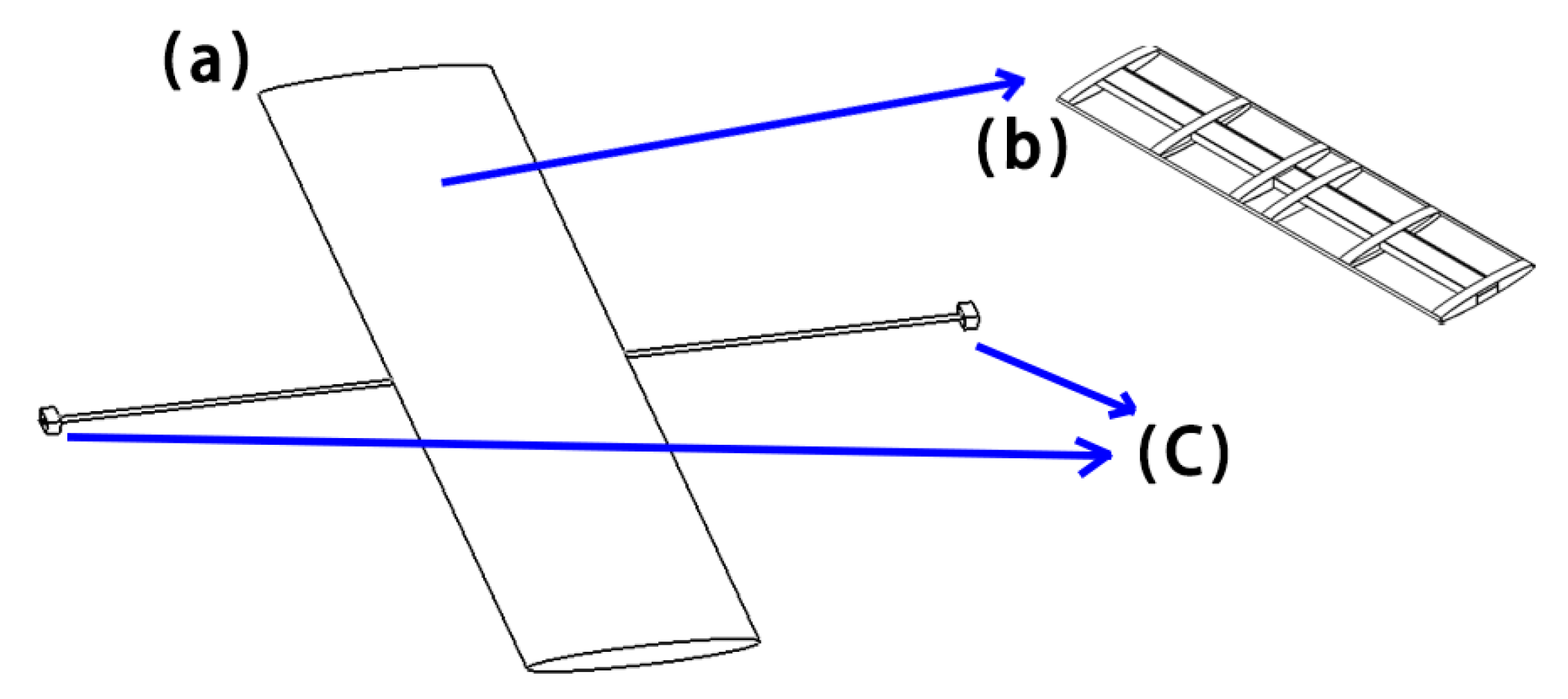
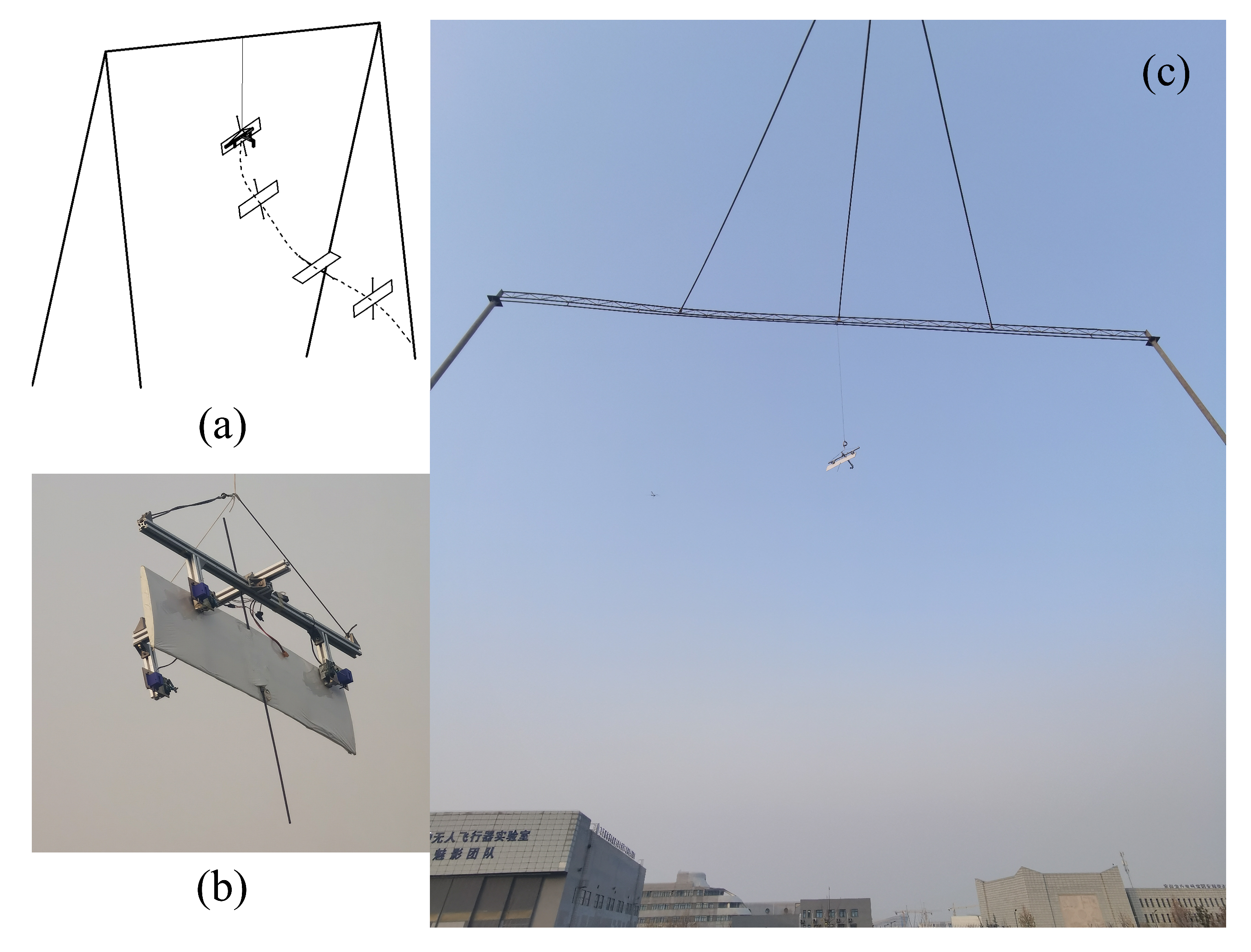
2.3. Experiment Method of Freely Falling Wing

In this section, an experimental method was designed for the freely falling wing. The experiments on a real wing verify the accuracy of the theoretical quasi-steady analytical model, and demonstrate the conclusions drawn from the analytical model and CFD numerical simulation. The experiment needs to measure the attitude and position of the wing’s movement. In previous studies on small objects such as paper and discs, high-speed photography technology has been used to record the falling trajectory of objects [44], and the experiments on freely falling objects are mostly carried out in narrow spaces such as water tanks. This is because the size of objects such as paper and discs is small, and the space required for the full development of the falling trajectory is also small. Related to the vision and lighting conditions, in this context, high-speed photography technology is not reliable. In prior research, the dynamic characteristics of plates can be measured by sensors including accelerometers, rategyros and magnetometers [45]. Therefore, in this study, the inertial measurement unit (IMU), shown in Figure 4, installed at the center of mass was used to measure the acceleration, attitude angle, and angular velocity of the wing. After filtering and integration, it was possible to obtain the falling path.
In order to easily change the MOI of the wing about the Y axis, a light thin stalk extends from the center of mass of the wing parallel to the chord. Metal clump weights with the same quality and shape are installed along the stalk, and the metal clump weights can be fixed at any position on the stalk. By making the clump weights and stalk symmetrical about the COM and by synchronously changing the position of the weights on the stalk, the MOI of the wing can be changed while keeping the mass and COM unchanged: see Figure 5.
However, it is very difficult to change the position of center of mass while keeping the moment of inertia unchanged. In order to change the position of COM, we adjusted the position of the weights on the stalk, but this will bring an obvious change of the inertia. Therefore, this work first researched the influence of the MOI on the freely falling wing, and then researched the effect of the COM position on falling motion. Finally, the total mass of the system was 253 g. The experimental procedure involved lifting the wing and release mechanism to a height, and releasing the wing free, as shown in Figure 6.

2.4. Validation and Discussion

To validate the quasi-steady analytical model and to improve the knowledge of the fluid field characteristics during the falling of the wing, this paper used CFD to numerically simulate the falling of a wing, with an initial attitude angle θ 0 = 75 . The results of the analytical model and CFD simulation as well as the experimental results are shown in Figure 7.
It can be seen that the analytical model can predict the angular motion well during the falling process, and also gives an accurate indication of the aerodynamic forces on the wing.
For further investigation, this paper used the Ω -method (a new generation vorticity identification method; refer to Appendix A.2 for details) to visualize vorticity around the falling wing simulated by CFD numerical calculations shown in Figure 8.
The process of the tumbling of the wing can be divided into two parts: a “transition phase” and a “stable tumbling phase”. In the transition phase, the wing is accelerated from the initial state, and the angular motion of the wing is not obvious while accelerating, mainly in translation motion. As the speed increases, the wing starts to tumble, and the vortex on the surface of the wing starts to shed, forming the vortex street. The frequency of vortex shedding is low in the transition phase. As the wing enters the stable tumbling stage, the frequency of vortex shedding accelerates and finally remains relatively stable.
The trend of the flow field during the transition phase of the example is shown in Figure 9. The formation of the vortex is similar to the results in Wan’s research [46]. Since the airfoil is symmetrical, the leading edge of the ellipse is defined as a side of the long-axis of the ellipse which is upwind and, similarly, the trailing edge can be defined as that downwind. In the later stage of the accelerated downward phase from the initial position, along with the pitching motion (Figure 9a), a vortex around the leading edge gradually forms and gradually strengthens; meanwhile, the force in the Z direction of the wing increases. When the pitch angle increases, the flow separates from the leading edge, but the vortex is still attached to the leading edge (Figure 9b), and the force in the Z direction peaks. The leading edge vortex then begins to shed (Figure 9c,d) at the same time as F z decreases, and an opposite separation vortex also appears at the trailing edge (Figure 9e). Due to the wing’s rotation, the original trailing edge became the current leading edge, and the circulation around the leading edge increases again (Figure 9e–h). As the wing maintains the rolling motion, the flow separates again at the leading edge with the separate vortex shedding out, similar to the process in Figure 9a–c. This tumbling motion is repeated for the subsequent transition phases of the wing.
In Figure 7, it can be observed that, during the early stages of the transition phase, the CFD simulation is closely aligned with the quasi-steady analytical model and the experiment method. During this period, the frequency of flow separation is relatively low, and there are no complex wake structures in the domain. However, the CFD model enters a steady tumbling motion after approximately 1 s (for a detailed explanation of the steady tumbling motion, refer to Section 3). This occurrence is relatively earlier compared to what is observed in the quasi-steady analytical model and experimental observations. It could be attributed to factors such as the approximation assumptions, numerical methods, and the boundary condition selection employed in the CFD model.

3. Effect of MOI

3.1. Quasi-Steady Analytical Model

Let the moment of inertia of the wing in the Y direction with units of kg·m 2 be set to 0.00045, 0.0006, 0.0008, 0.001, 0.002, 0.004, 0.006, 0.008, and 0.009, respectively, while the mass and shape of the wing remain unchanged. By substituting these states into the quasi-steady analytical model and simulating at the same initial state, the trajectory of the freely falling wing can be observed as shown in Figure 10. In order to more clearly illustrate the simulation of the wing tumbling process, the change in orientation of the wing in the free-fall path is shown in Figure 11. This is similar to the observations made by Andersen et al. in a small, freely falling plate, as reported in [24].
As can be gleaned from Figure 10 and Figure 11, it is evident that, as the MOI about the Y -axis of the wing increases, the falling trajectory of the wing becomes steeper, resulting in a greater loss of height. Concurrently, the angular rate of tumbling θ ˙ of the wing also decreases. In the phase diagrams of Figure 11b,e, the tumbling of the wing exhibits stable limit cycle oscillation. After entering the falling motion, the phase trajectory from the initial state is attracted to the limit cycle, eventually undergoing periodic motion within the limit cycle. As the moment of inertia (MOI) of the wing increases, the process of convergence from the initial state to the limit cycle becomes more protracted. In phase space, the phase locus takes longer to converge to the limit cycle in the θ ˙ direction relative to the v x , v z direction, and the average angular velocity decreases, which is a consequence of the increased MOI. From Equation (5), it can be deduced that the circulation generated by the angular motion decreases, resulting in a decrease in F z , thereby augmenting the sink rate of the wing.

3.2. Experiment Results

The falling experiment was conducted using the experimental setup depicted in Figure 5 and Figure 6. The position of the clump weights were adjusted to alter the wing’s moment of inertia (MOI), and the wing was released at a height of 5 m with an initial attitude angle of θ 0 = 75 . The acceleration, angular velocity, and attitude angle were measured using an inertial measurement unit (IMU) and they were used to derive the trajectory of the wing’s descent, as shown in Figure 12. The external forces acting on the wing were also estimated.
It can be seen that, as the wing’s MOI increases, the falling trajectory becomes steeper and the transition phase from the beginning of the fall to the stable tumbling phase becomes longer, which is consistent with the conclusions obtained from the analytical model in the previous sections. The experimental results also indicate that the analytical model can accurately predict the tumbling behavior of a freely falling wing. This is likely due to the fact that some of the coefficients in the analytical model are determined by experiments conducted in previous work, allowing the model to capture some of the three-dimensional effects during the falling motion. However, discrepancies between the simulated and experimental data may be attributed to sensor noise, the analytical model’s inability to account for complex nonlinear and unsteady aerodynamic effects, and external perturbations in the falling experiment. The wing tumbling motion in the experiment, shown in Figure 12, did not occur strictly in the two-dimensional plane, also due to these perturbations.

4. Effect of COM Position on Freely Falling Wing

The coordinate system O X c l u m p is established at the center of the stalk in Figure 3, with the O X c l u m p axis aligned with the O X axis. The coordinates of the two clump weights on the O X c l u m p axis are denoted as C x l and C x r , respectively.
By altering the relative position of the counterweight on the stalk in Figure 3, the position of the COM can be adjusted while maintaining the mass constant. The relationship between the clump weights’ position, the COM position X c , and the moment of inertia I c is presented in Table 1:

4.1. Simulation of the Analytical Model

By incorporating the above model parameters into the analytical model, the simulation trajectory can be obtained, as depicted in Figure 13. The phase diagrams of the freely falling wing’s v x , v z , and θ ˙ can also be generated.
According to the simulation results, it can be observed that, as the COM position moves forward, the transition phase from the initial state to the limit cycle of tumbling motion takes longer and the phase trajectory of the transition phase becomes more complex. As seen in Figure 13, when the COM position is shifted approximately 40 mm from the geometric center of the wing, corresponding to case 5, a new limit cycle appears in the phase space. The projection of the phase trajectory in the v x , v z plane and the v z , θ ˙ plane in Figure 13f is shown in Figure 14, respectively. It can be observed that the curve starts from the initial state and quickly enters the new limit cycle, undergoing quasi-periodic motion in the ring. The stability of the v x , v z direction within the limit cycle is evident, while the θ ˙ direction is not stable. As a result, the phase trajectory eventually leaves the new limit cycle as the number of oscillations increases, as shown in Figure 14b. After leaving the new limit cycle, the curve is attracted to the limit cycle corresponding to the original tumbling motion and eventually converges to this limit cycle. The falling motion of the wing is characterized by initial fluttering, with the flutter angular velocity’s amplitude increasing before the wing enters the tumbling falling phase. The trajectory of the wing’s fall is depicted in Figure 15. Figure 15a shows the fluttering of the wing during the fall represented by the newly emerged limit cycle, and Figure 15b shows the transition from fluttering to tumbling motion. As the COM moves further forward, the limit cycle corresponding to the tumbling motion disappears and the wing falls while fluttering periodically according to the limit cycle shown in Figure 13g.

4.2. Experiment Results

In this part, the experimental method was employed to observe the actual falling trajectory of the wing after release. Using the wing shown in Figure 3, the position of the clump weights block is varied according to the scheme in Table 1, and the falling experiments are conducted for Case 1 to Case 6, respectively. The measured falling trajectory of the wing is shown in Figure 16.
In the experiment, due to the asymmetrical disturbance on the wing, the actual falling trajectory is difficult to maintain in the X Z plane, and the wing typically falls along a helix. The tumbling motion is depicted in Figure 16 as the wing tumbles around the Y axis of the body coordinate system in the helix. It can be seen that, for case 1 to case 5 (Figure 16a–e), the tumbling motion occurs before the wing touches the ground, with the transition phase from the initial state to the tumbling motion of the wing becoming longer as the position of the COM moves forward. However, for case 6 (Figure 16f), the wing does not tumble until it touches the ground and falls more smoothly along the helix. Projecting the spiral line falling trajectory in the transition phase of the wing into the two-dimensional plane is similar to the trajectory corresponding to case 5 in Figure 15, which demonstrates a heaving/pitching composite motion along the spiral line in the actual three-dimensional motion. The discrepancy between the experimental trajectory and the trajectory simulated by the two-dimensional analytical model is attributed to the asymmetry of the wing, the asymmetry of external disturbance, and the asymmetrical shedding of vortex on the wing surface during the actual falling process.

5. Results and Discussion

5.1. Quasi-Steady Analytical Model Results

1.
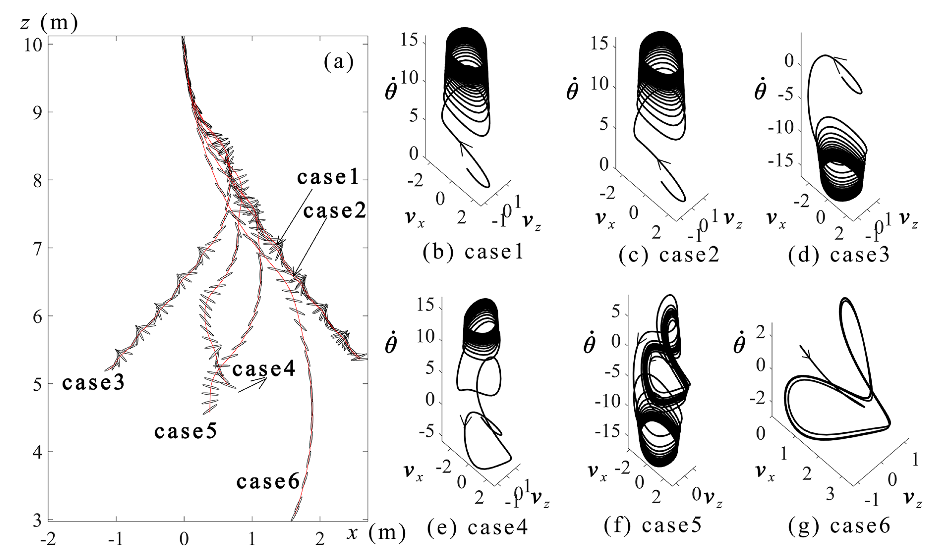
Effect of MOI: In the case of wings with different MOIs, there exists a limit cycle of tumbling motion that all wings will eventually converge to after releasing, reaching a stable state shown in Figure 11. The phase from the initial state to the final stable tumbling limit cycle is defined as the transition phase. As the MOI of the wing increases, the trajectory of the free-falling wing becomes steeper, and the transition phase becomes longer, meaning that the wing will take more time to converge to the limit cycle.
2.
Effect of COM: When the COM moves forward, the transition phase from the initial state to the tumbling motion limit cycle becomes longer, and the phase trajectory during the transition phase becomes more complex. A new limit cycle emerges when the COM is positioned 40 mm ahead of the wing’s geometric center, as can be seen in Figure 13f, corresponding to the quasi-periodic fluttering motion of the wing. At this point, the limit cycle of the fluttering motion is unstable, and the phase trajectory eventually diverges from this limit cycle, converging towards the limit cycle of the tumbling motion; Figure 15 shows this process well. As the COM continues to move forward, the limit cycle corresponding to the tumbling motion disappears, and the limit cycle of the fluttering motion becomes a stable limit cycle, resulting in the wing freely falling with periodic fluttering motion.

5.2. Experimental Results

1.
Effect of MOI: By symmetrically altering the position of the clump weights block, the MOI of the wing is changed, and tumbling motion is observed under different conditions of MOI, as shown in Figure 12. As the MOI of the wing increases, the trajectory of the freely falling wing becomes steeper, and the transition phase from the initial descent to stable tumbling becomes longer. This observation aligns with the conclusions drawn from the analytical model.
2.
Effect of COM: Experimental results show that maintaining the actual wing trajectory in the X Z plane is challenging because of asymmetrical disturbances. Typically, the wing descends along a spiral path, as shown in Figure 16. As the COM moves forward, the transition phase from the initial state to tumbling motion increases. Further forward movement of the COM results in the fluttering motion of the wing. However, no tumbling motion is observed in the experiment after shifting the COM forward by 40 mm, as shown in Figure 16d.

5.3. Comparison of the Analytical Model with Experimental Results

The quasi-steady analytical model accurately reveals the influence of changes in MOI and COM on the freely falling motion of the wing. These observed motion patterns are consistent with the conclusions obtained from the quasi-steady analytical model. However, due to unavoidable asymmetrical disturbances on the wing during experiments, maintaining the wing’s trajectory within a two-dimensional plane becomes challenging. Additionally, obtaining an accurate trajectory of the wing is difficult due to sensor errors.

6. Conclusions

In this study, the dynamics of a freely falling wing in the context of air-drop launch technology for UAVs was investigated. The mass, MOI, and COM position of the wing have a significant impact on the flight characteristics of UAVs; thus, this study examined the effect of changes in the moment of inertia and center of mass position on the falling motion while holding the mass constant. The aerodynamic forces acting on a freely falling wing are complex, nonlinear, and unsteady, and exhibit strong coupling with the wing motion, making them challenging to accurately model numerically. Extensive research has been conducted on the dynamics of falling objects, resulting in the development of various numerical simulation methods and simplified descriptive models. However, these studies largely focus on the free-fall of small objects with simple geometric shapes such as flat plates and discs in a laboratory setting, rather than larger objects such as wings. In this study, the Andersen–Pesavento–Wang analytical model was adapted to the analysis of the freely falling wing, and a correction term was added to account for the center of mass position. The quasi-steady analytical model was validated by CFD and experimental results. This study investigated the effects of the MOI and COM position on the dynamics of a freely falling wing, and drew the following conclusions:
1.
A quasi-steady analytical model was developed based on the Andersen–Pesavento–Wang model. The analytical model was derived in the two-dimensional plane and can reflect the dynamic behavior well in the longitudinal plane during the three-dimensional falling of a real wing.
2.
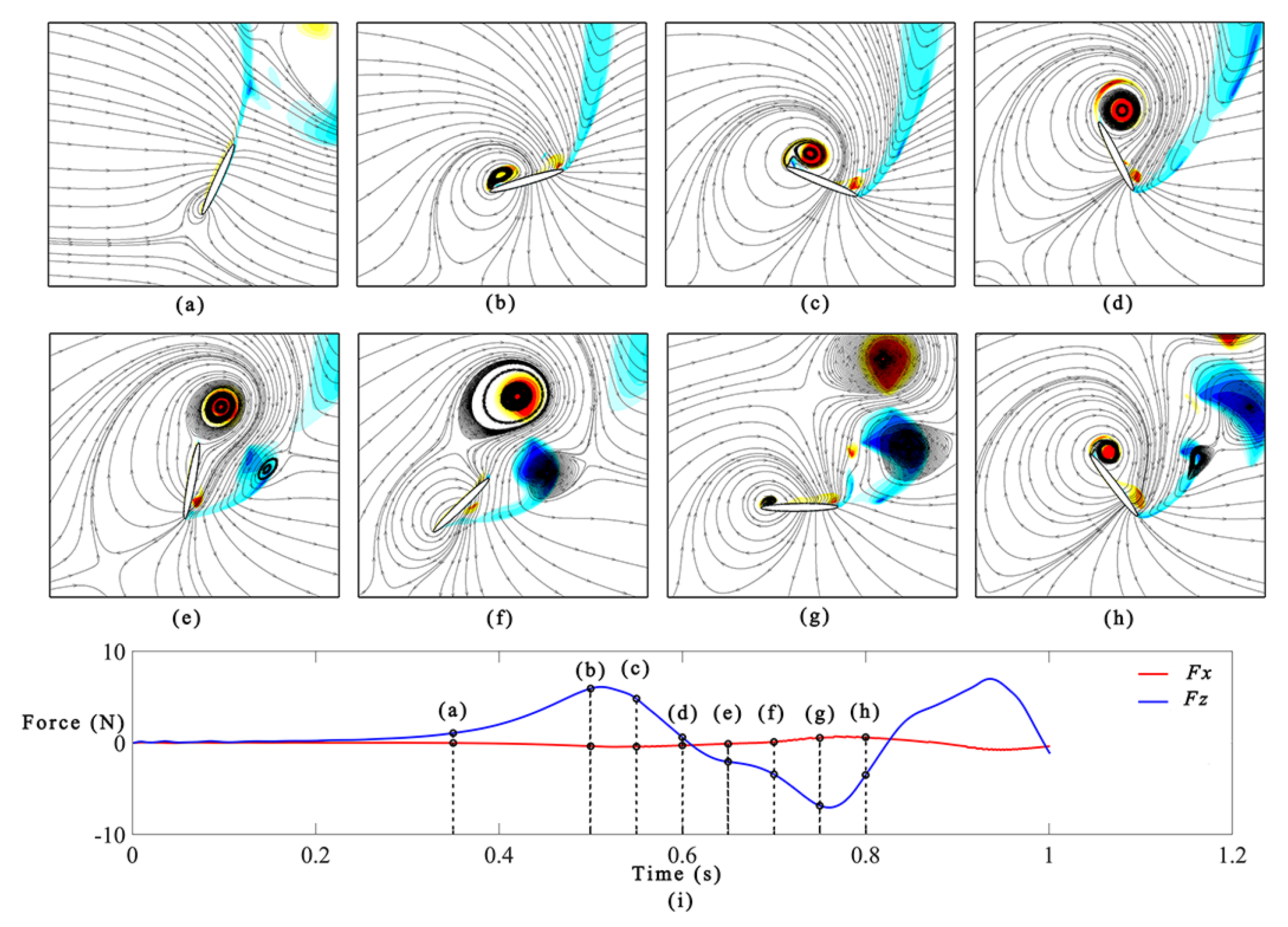
After deployment, the wing undergoes a transition phase before eventually entering a stable motion, which can be characterized as either tumbling or fluttering, as revealed by the quasi-steady analysis model and experiment method employed in this study. Through CFD analysis, it is observed that, during the transition phase, the shedding frequency of vortices gradually increases and stabilizes, resulting in periodic aerodynamic oscillations due to the cyclic generation and separation of vortices. These periodic oscillations eventually lead to the emergence of a stable periodic motion. Both of these stable motions exhibit relatively low translational velocities. In the case of rolling motion, the pitch rate of the wing remains approximately 15 rad/s. In the case of fluttering motion, the pitch rate oscillates between positive and negative values. Therefore, both of these stable motion patterns should be avoided in the air-drop launched UAVs.
3.
For a wing with elliptical airfoil, the higher the MOI about the Y -axis, the steeper the trajectory, the lower the angular rate of tumbling, and the shorter time for it staying in the air. For most aircraft, the pitch tumbling is not beneficial. Without changing the shape of the wing and the position of the COM, and only changing the MOI of the wing about the Y -axis, the initial drop attitude cannot prevent the pitch tumbling of the wing during the falling process.
4.
The position of the COM has a crucial influence on the handling performance and stability of the UAVs. The traditional flight dynamics theory suggests that the forward shift of the COM position can make the vehicle obtain better static stability. For the freely falling wing, the forward shift of the COM will delay the appearance of tumbling, i.e., the transition phase becomes longer. When the forward shift of the COM exceeds a certain value, a new relatively stable motion of falling appears, which is expressed as fluttering in the analytical model, while the wing shows a heaving/ pitching composite motion along the spiral line in the real three-dimensional falling experiment. In the future, for air-drop launch UAVs with relaxed longitudinal static stability, the possibility of its tumbling needs to be considered.
In the future, the analytical model can be considered to include corrections for different airfoil types and wing shapes, and to include the effects of rudder surfaces, so that the model can describe the freely falling process of a more general aircraft. Since the model also uses two-dimensional quasi-steady assumptions, extending the model to three-dimensional space and considering the unsteady aerodynamic force for better prediction of falling motion is worth studying. In addition, the analysis of the uncertainties of this complex process is a research direction of interest.

Author Contributions

Conceptualization, Y.D.; methodology, Y.D.; software, Y.D.; validation, K.W. and W.D.; formal analysis, K.W. and Y.D.; investigation, Y.D. and K.W.; resources, Y.D.; data curation, Y.D., Z.S. and W.D.; writing—original draft preparation, Y.D. and K.W.; writing—review and editing, K.W. and P.R.T.; visualization, K.W.; supervision, K.W.; project administration, Z.Z.; funding acquisition, Z.Z. All authors have read and agreed to the published version of the manuscript.

Funding

This research was funded by Natural Science Foundation of Shaanxi Province OF FUNDER grant number 2023-JC-QN-0043.

Data Availability Statement

The data can be provided on request.

Conflicts of Interest

The authors declare no conflict of interest.

Abbreviations

CFDComputational Fluid Dynamics
COMCenter of Mass
DOAJDirectory of open access journals
LDLinear dichroism
MDPIMultidisciplinary Digital Publishing Institute
MOIMoment of Inertia
TLAThree Letter Acronym
UAVUnmanned Aerial Vehicle
Symbols
aSemimajor axis of the ellipse (m)
bSemiminor axis of the ellipse (m)
eEccentricity of the airfoil
F x v Translational drag force in the X direction (N)
F z v Translational drag force in the Z direction (N)
Γ Circulation (m 2 /s)
gGravitational acceleration (m/s 2 )
IMoment of inertia about the Y -axis (kg·m 2 )
JAdded moment of inertia (kg·m 2 )
l τ Length of the torque arm (m)
mMass of the wing (kg)
m x Added mass coefficient in the X direction
m z Added mass coefficient in the Z direction
ρ f Density of the air (kg/m 3 )
ρ s Density of the wing (kg/m 3 )
ρ θ Volume density of the fluid displaced by the wing (kg/m 4 )
τ θ Torque about the Y -axis (N m)
v x Speed in the X direction of the body coordinate system (m/s)
v z Speed in the Z direction of the body coordinate system (m/s)
Subscripts
CCentroid
fZone of fluid
sZone of wing
X X direction of the body coordinate system
Y Y -axis vertical to the X O Z plane
Z Z direction of the body coordinate system

Appendix A. Method Description

Appendix A.1. Range-Kutta Method

The general form of the fourth-order Range-Kutta method can be expressed as:
y n + 1 = y n + h 6 ( k 1 + 2 k 2 + 2 k 3 + k 4 ) k 1 = f ( t n , y n ) k 2 = f ( t n + 1 2 h , y n + 1 2 h k 1 ) k 3 = f ( t n + 1 2 h , y n + 1 2 h k 2 ) k 4 = f ( t n + h , y n + h k 3 )
Here, y n represents the numerical approximation of the solution at time step t n . The function f corresponds to the derivative function that needs to be solved. The parameter h denotes the step size, while k 1 through k 4 are intermediate values computed at different points using the function f.

Appendix A.2. The Ω-Method Vortex Identification Criterion

Ω -method is considered as a new generation vorticity identification method [47], the Ω -method can be expressed as:
V = 1 2 ( V + V T ) + 1 2 ( V V T ) = A + B
where V denotes the velocity vector, and let
a = t r a c e ( A T A ) = i = 1 3 j = 1 3 ( A i j ) 2 b = t r a c e ( B T B ) = i = 1 3 j = 1 3 ( B i j ) 2
The final form of Ω -method can be written as:
Ω = b a + b + ε
The Ω -method exhibits the feature of normalized threshold, setting it apart from other methods such as vorticity field and Q-criterion, which necessitate the adjustment of various thresholds. In the Ω -method, the thresholds are normalized within the range of 0 to 1. As a result, the Ω -method is regarded as a comprehensive approach capable of effectively highlighting both strong and weak vortices.

References

  1. Tao, T.S. Design and Development of a High-Altitude, In-Flight-Deployable Micro-UAV; MIT Lincoln Laboratory: Cambridge, MA, USA, 2013. [Google Scholar]
  2. Ye, S.-C.; Yao, X.X. On the Other-Power Launch Technology of Unmanned Aerial Vehicles. J. Command Control 2018, 4, 15–21. [Google Scholar]
  3. Hu, Y.; Yang, Y.; Ma, X.; Li, S. Computational optimal launching control for balloon-borne solar-powered unmanned aerial vehicles in near-space. Sci. Prog. 2020, 103, 0036850419877755. [Google Scholar] [CrossRef] [PubMed]
  4. Zhu, Z.; Guo, H.; Ma, J. Aerodynamic layout optimization design of a barrel-launched UAV wing considering control capability of multiple control surfaces. Aerosp. Sci. Technol. 2019, 93, 105297. [Google Scholar] [CrossRef]
  5. Wang, Y.; Yang, C.; Yang, H. Neural network-based simulation and prediction of precise airdrop trajectory planning. Aerosp. Sci. Technol. 2022, 120, 107302. [Google Scholar] [CrossRef]
  6. Wu, M.; Shi, Z.; Xiao, T.; Ang, H. Effect of wingtip connection on the energy and flight endurance performance of solar aircraft. Aerosp. Sci. Technol. 2021, 108, 106404. [Google Scholar] [CrossRef]
  7. Guo, A.; Zhou, Z.; Zhu, X.; Zhao, X. Coupled Flexible and Flight Dynamics Modeling and Simulation of a Full-Wing Solar-Powered Unmanned Aerial Vehicle. J. Intell. Robot. Syst. 2021, 101, 56. [Google Scholar] [CrossRef]
  8. Wu, M.; Shi, Z.; Xiao, T.; Ang, H. Energy optimization and investigation for Z-shaped sun-tracking morphing-wing solar-powered UAV. Aerosp. Sci. Technol. 2019, 91, 1–11. [Google Scholar] [CrossRef]
  9. Acosta, G.; Hassanalian, M. Power minimization of fixed-wing drones for Venus exploration in various altitudes. Acta Astronaut. 2020, 180, 1–15. [Google Scholar] [CrossRef]
  10. Hu, Y.; Guo, J.; Meng, W.; Liu, G.; Xue, W. Longitudinal control for balloon-borne launched solar powered UAVs in near-space. J. Syst. Sci. Complex. 2022, 35, 802–819. [Google Scholar] [CrossRef]
  11. Gevers, D.E.; Ratcliff, M.M.; Hatch, J.A. Balloon Launched UAV with Nested Wing for near Space Applications; Technical Report, SAE Technical Paper; SAE: Warrendale, PA, USA, 2007. [Google Scholar]
  12. Doi, H. Tacom-air-launched multi-role UAV. In Proceedings of the 24th Congress of International Council of the Aeronautical Sciences, Yokohama, Japan, 29 August–3 September 2004. [Google Scholar]
  13. Wynsberghe, E.V.; Turak, A. Station-keeping of a high-altitude balloon with electric propulsion and wireless power transmission: A concept study. Acta Astronaut. 2016, 128, 616–627. [Google Scholar] [CrossRef]
  14. Wang, X.; Zeng, G.; Yan, X.; Chen, W.; Li, K.; Yang, Y. A Feasibility Verification Scheme with Flight Analysis for Balloon-borne Launched Unmanned Aerial Vehicles. In Proceedings of the 2020 3rd International Conference on Unmanned Systems (ICUS), Harbin, China, 27–28 November 2020; pp. 966–971. [Google Scholar]
  15. Fang, R.; Zhang, Y.; Liu, Y. Aerodynamics and flight dynamics of free-falling ash seeds. World J. Eng. Technol. 2017, 5, 105–116. [Google Scholar] [CrossRef]
  16. Sohn, M.H.; Im, D.K. Flight characteristics and flow structure of the autorotating maple seeds. J. Vis. 2022, 25, 483–500. [Google Scholar] [CrossRef]
  17. Arranz, G.; Moriche, M.; Uhlmann, M.; Flores, O.; García-Villalba, M. Kinematics and dynamics of the auto-rotation of a model winged seed. Bioinspir. Biomim. 2018, 13, 036011. [Google Scholar] [CrossRef] [PubMed]
  18. Yue, S.; Nie, H.; Zhang, M.; Wei, X.; Gan, S. Design and landing dynamic analysis of reusable landing leg for a near-space manned capsule. Acta Astronaut. 2018, 147, 9–26. [Google Scholar] [CrossRef]
  19. Pandula, Z.; Kullmann, L.; Hos, C. Analysis of the Free-Fall of a Disc in Viscous Fluid Using the Techniques of Nonlinear Dynamics. 2002. Available online: https://www.researchgate.net/profile/Csaba-Hos/publication/228585874_Analysis_of_the_free-fall_of_a_disc_in_viscous_fluid_using_the_techniques_of_nonlinear_dynamics/links/5615582a08ae4ce3cc652f6d/Analysis-of-the-free-fall-of-a-disc-in-viscous-fluid-using-the-techniques-of-nonlinear-dynamics.pdf (accessed on 11 December 2002).
  20. Maxwell, J.C. On a particular case of the descent of a heavy body in a resisting medium. Camb. Dublin Math. J. 1854, 9, 145–148. [Google Scholar]
  21. Willmarth, W.W.; Hawk, N.E.; Harvey, R.L. Steady and unsteady motions and wakes of freely falling disks. Phys. Fluids 1964, 7, 197–208. [Google Scholar] [CrossRef]
  22. Smith, E. Autorotating wings: An experimental investigation. J. Fluid Mech. 1971, 50, 513–534. [Google Scholar] [CrossRef]
  23. Field, S.B.; Klaus, M.; Moore, M.; Nori, F. Chaotic dynamics of falling disks. Nature 1997, 388, 252–254. [Google Scholar] [CrossRef]
  24. Andersen, A.; Pesavento, U.; Wang, Z.J. Unsteady aerodynamics of fluttering and tumbling plates. J. Fluid Mech. 2005, 541, 65–90. [Google Scholar] [CrossRef]
  25. Lam, T.; Vincent, L.; Kanso, E. Passive flight in density-stratified fluids. J. Fluid Mech. 2019, 860, 200–223. [Google Scholar] [CrossRef]
  26. Esteban, L.B.; Shrimpton, J.; Ganapathisubramani, B. Three dimensional wakes of freely falling planar polygons. Exp. Fluids 2019, 60, 114. [Google Scholar] [CrossRef]
  27. Toupoint, C.; Ern, P.; Roig, V. Kinematics and wake of freely falling cylinders at moderate Reynolds numbers. J. Fluid Mech. 2019, 866, 82–111. [Google Scholar] [CrossRef]
  28. You, C.S.; Chern, M.J.; Noor, D.Z.; Horng, T.L. Numerical investigation of freely falling objects using direct-forcing immersed boundary method. Mathematics 2020, 8, 1619. [Google Scholar] [CrossRef]
  29. Kim, J.T.; Jin, Y.; Shen, S.; Dash, A.; Chamorro, L.P. Free fall of homogeneous and heterogeneous cones. Phys. Rev. Fluids 2020, 5, 093801. [Google Scholar] [CrossRef]
  30. Tam, D.; Bush, J.W.; Robitaille, M.; Kudrolli, A. Tumbling dynamics of passive flexible wings. Phys. Rev. Lett. 2010, 104, 184504. [Google Scholar] [CrossRef]
  31. Esteban, L.B.; Shrimpton, J.; Ganapathisubramani, B. Edge effects on the fluttering characteristics of freely falling planar particles. Phys. Rev. Fluids 2018, 3, 064302. [Google Scholar] [CrossRef]
  32. Esteban, L.; Shrimpton, J.; Ganapathisubramani, B. Disks settling in turbulence. J. Fluid Mech. 2020, 883, A58. [Google Scholar] [CrossRef]
  33. Howison, T.; Hughes, J.; Iida, F. Large-scale automated investigation of free-falling paper shapes via iterative physical experimentation. Nat. Mach. Intell. 2020, 2, 68–75. [Google Scholar] [CrossRef]
  34. Lee, M.; Lee, S.H.; Kim, D. Stabilized motion of a freely falling bristled disk. Phys. Fluids 2020, 32, 113604. [Google Scholar] [CrossRef]
  35. Zhou, X.; Yuan, S.; Zhang, G. Eccentric disks falling in water. Phys. Fluids 2021, 33, 033325. [Google Scholar] [CrossRef]
  36. Kozlov, V.V. On the problem of fall of a rigid body in a resisting medium. Vestnik Moskov. Univ. Ser. I Mat. Mekh. 1990, 79–86. [Google Scholar]
  37. Tanabe, Y.; Kaneko, K. Behavior of a falling paper. Phys. Rev. Lett. 1994, 73, 1372. [Google Scholar] [CrossRef] [PubMed]
  38. Belmonte, A.; Eisenberg, H.; Moses, E. From flutter to tumble: Inertial drag and Froude similarity in falling paper. Phys. Rev. Lett. 1998, 81, 345. [Google Scholar] [CrossRef]
  39. Andersen, A.; Pesavento, U.; Wang, Z.J. Analysis of transitions between fluttering, tumbling and steady descent of falling cards. J. Fluid Mech. 2005, 541, 91–104. [Google Scholar] [CrossRef]
  40. Wang, K.; Zhou, Z. An investigation on the aerodynamic performance of a hand-launched solar-powered UAV in flying wing configuration. Aerosp. Sci. Technol. 2022, 129, 107804. [Google Scholar] [CrossRef]
  41. Sedov, L.I. Two-dimensional problems of hydrodynamics and aerodynamics. Mosc. Izd. Nauka 1980. [Google Scholar]
  42. Wang, Z.J.; Birch, J.M.; Dickinson, M.H. Unsteady forces and flows in low Reynolds number hovering flight: Two-dimensional computations vs robotic wing experiments. J. Exp. Biol. 2004, 207, 449–460. [Google Scholar] [CrossRef]
  43. Kuznetsov, S.P. Plate falling in a fluid: Regular and chaotic dynamics of finite-dimensional models. Regul. Chaotic Dyn. 2015, 20, 345–382. [Google Scholar] [CrossRef]
  44. Zakaria, M.Y.; Dos Santos, C.R.; Dayhoum, A.; Marques, F.; Hajj, M.R. Modeling and prediction of aerodynamic characteristics of free fall rotating wing based on experiments. In Proceedings of the International Conference on Aerospace Sciences and Aviation Technology, Cairo, Egypt, 9–11 April 2019; The Military Technical College: Cairo, Egypt, 2019; Volume 18, pp. 1–15. [Google Scholar]
  45. Rostami, A.B.; Fernandes, A.C. Mathematical model and stability analysis of fluttering and autorotation of an articulated plate into a flow. Commun. Nonlinear Sci. Numer. Simul. 2018, 56, 544–560. [Google Scholar] [CrossRef]
  46. Wan, H.; Dong, H.; Liang, Z. Vortex formation of freely falling plates. In Proceedings of the 50th AIAA Aerospace Sciences Meeting Including the New Horizons Forum and Aerospace Exposition, Nashville, Tennessee, 9–12 January 2012; p. 1079. [Google Scholar]
  47. Liu, C.; Wang, Y.; Yang, Y.; Duan, Z. New omega vortex identification method. Sci. China Phys. Mech. Astron. 2016, 59, 684711. [Google Scholar] [CrossRef]
Figure 1. The design of the wing and the coordinate system definition of the model.
Aerospace 10 00458 g001
Figure 2. The computational mesh around the wing (2D view).
Aerospace 10 00458 g002
Figure 3. Two-dimensional CFD calculation mesh (a) Complete domain (b) Partial enlarged view of overset component.
Aerospace 10 00458 g003
Figure 4. The WT901 inertial measurement unit. WT901 has a mass of 20 g and is able to transmit data via WiFi with a transmission frequency of 200 Hz.
Aerospace 10 00458 g004
Figure 5. (a) Wing and clump weights assembly. (b) The inner structure of the wing. (c) Clump weights.
Aerospace 10 00458 g005
Figure 6. (a) Experimental scheme for freely falling wing. (b) Wing and release system. (c) Wing free-fall experimental platform.
Aerospace 10 00458 g006
Figure 7. Comparison of simulation data with experimental data for pitch angle θ , x -directional force F x , and z -directional force F z simulated by the analytical model and CFD, where (I = 0.00045 kg·m 2 ).
Aerospace 10 00458 g007
Figure 8. The vorticity street around the freely falling wing. Positive vortices are red and negative vortices are blue (ad), respectively, represent the distribution of vortices on the falling trajectory of the wing with different MOIs in two seconds, where the unit of I is kg·m 2 .
Aerospace 10 00458 g008
Figure 9. Streamline diagram of the first one second in the transition phase of the wing for (I = 0.00045 kg·m 2 ), with vortex contour with force change curve. (ah) Vortical contour ( Ω -criterion) and streamline around the wing: positive vortices are in red and negative vortices are in blue. (i) Aerodynamic forces in x and z directions.
Aerospace 10 00458 g009
Figure 10. Simulation of falling trajectories of airfoils with different MOIs using the analytical model, where the unit of I is kg·m 2 .
Aerospace 10 00458 g010
Figure 11. The trajectory obtained from the analytical model and its ( v x , v z , θ ˙ ) phase diagram. (a) Trajectory visualization for the simulation of freely falling wings with different MOIs, (be) Extend the simulation time to 20 s and make the ( v x , v z , θ ˙ ) phase diagram, where the unit of I is kg·m 2 .
Aerospace 10 00458 g011
Figure 12. The trajectory of the freely falling wing with different MOIs observed in the experiment, where the unit of I is kg·m 2 .
Aerospace 10 00458 g012
Figure 13. The falling trajectory and phase diagram as predicted by the analytical model. (a) The falling trajectories corresponding to the six cases in Table 1. (bg) The plots of ( v x , v z , θ ˙ ) phase diagrams for the six cases over a simulation time of 20 s. The units of the linear velocities V x and V z are m/s, and the unit of angular velocity θ ˙ is rad/s.
Aerospace 10 00458 g013
Figure 14. Phase diagram and the projection of the phase trajectory for case 5 in two planes. (a) Phase diagram for case 5. (b) Projection of the phase trajectory in the v z , θ ˙ plane. (c) Projection of the phase trajectory in the v x , v z plane. The units of the linear velocities V x and V z are m/s, and the unit of angular velocity θ ˙ is rad/s.
Aerospace 10 00458 g014
Figure 15. The simulation results for case 5 as predicted by the quasi-steady model: (a) Local magnification of the drop trajectory when the wing exhibits fluttering behavior. (b) Local magnification of the drop trajectory showing the transformation of the wing from fluttering to tumbling.
Aerospace 10 00458 g015
Figure 16. The free−falling trajectory of the wing after altering the position of the COM in the experiment. (a) Flight trajectory for case 1. (b) Flight trajectory for case 2. (c) Flight trajectory for case 3. (d) Flight trajectory for case 5. (e) Flight trajectory for case 4. (f) Flight trajectory for case 6.
Aerospace 10 00458 g016
Table 1. The relationship between the coordinates of the clump weights, the COM position, and the MOI.
Case C xl (mm) C xr (mm) X c (mm) I c (kg·m 2 )
1−4005004.5470.008
2−30050010.1260.007
3−12550019.890.006
410050032.440.006
525050040.8130.006
640050049.1380.008
Disclaimer/Publisher’s Note: The statements, opinions and data contained in all publications are solely those of the individual author(s) and contributor(s) and not of MDPI and/or the editor(s). MDPI and/or the editor(s) disclaim responsibility for any injury to people or property resulting from any ideas, methods, instructions or products referred to in the content.

