Article

Identification of Lateral-Directional Aerodynamic Parameters for Aircraft Based on a Wind Tunnel Virtual Flight Test

1
School of Aeronautic Science and Engineering, Beihang University, Beijing 100191, China
2
AVIC Aerodynamics Research Institute, Harbin 150001, China
*
Author to whom correspondence should be addressed.
Aerospace 2023, 10(4), 350; https://doi.org/10.3390/aerospace10040350
Submission received: 11 March 2023 / Revised: 25 March 2023 / Accepted: 27 March 2023 / Published: 3 April 2023
(This article belongs to the Special Issue Flight Dynamics, Control & Simulation)

Abstract

:
In the early stages of aircraft design, a scaled model of the aircraft is installed in a wind tunnel for dynamic semi-free flight to approximate real flight, and the test data are then used to identify the aerodynamic parameters. However, the absence of the translational motion of the test model makes its flight dynamics different from those in free flight, and the effect of this difference on parameter identification needs to be investigated. To solve this problem, a 3-DOF wind tunnel virtual flight test device is built to fix the test model on a rotating mechanism, and the model is free to rotate in three axes through the deflection of the control surfaces. The flight dynamics equations for the wind tunnel virtual flight test are established and expressed as a decoupled form of the free flight force and the influence of the test support frame force on the model’s motions through linearization. The differences between wind tunnel virtual flight and free flight are analysed to develop a model for the identification of aerodynamic parameters. The selection of the lateral-directional excitation signal and the design method of its parameters are established based on the requirements for the identifiability of the aerodynamic derivatives, and a step-by-step method for the identification of aerodynamic force and moment derivatives is established. The aerodynamic parameter identification results of a blended wing body aircraft show that the identification method proposed in this paper can obtain results with high accuracy, and the response of the modified motion model is consistent with that of the free flight motion model.

1. Introduction

The identification of aerodynamic parameters and the study of the dynamics of aircraft based on actual test flights of real aircraft is costly and risky [1,2]. In the early stage of aircraft design, a wind tunnel virtual flight test is carried out to fly the test model dynamically in the wind tunnel, and then complete the identification of aerodynamic parameters and compare and correct with the traditional wind tunnel force measurement data [3,4].
At present, the most widely used wind tunnel virtual flight test is a dynamic flight test with three degrees of freedom [5]. As shown in Figure 1, in the wind tunnel virtual flight test, the test model is connected with the support rod through a three-degree-of-freedom rotating mechanism and installed in the wind tunnel test section, so that the linear displacement of the model is fixed, but it has three angular motion degrees of freedom. Open-loop and closed-loop control of the test model are achieved by driving the control surface directly or by using the flight control law to drive the control surface, respectively [6].
The traditional wind tunnel test and aerodynamic modelling technology are based on the linear superposition principle [7], as shown in Figure 2. Static wind tunnel tests are used to obtain constant aerodynamic data, small amplitude forced oscillation tests are used to obtain dynamic derivative data, and the large-amplitude forced oscillation test is used to obtain aerodynamic data at a large angle of attack, so that the aerodynamic model of the aircraft can be finally constructed [8].
Traditional wind tunnel force measurements are sometimes inaccurate. The traditional wind tunnel test technique decomposes the parameters of aircraft motion and attitude to study them, which separates the interaction and influence between aerodynamics and motion, and the test results obtained cannot fully reflect the aerodynamic characteristics during real flight. Particularly in the large angle of attack, the aircraft’s translation, rotation, and control surface deflection are coupled with each other, when the traditional wind tunnel measurement results often differ from the aerodynamic model of real flight. Data from wind tunnel virtual flight tests can be used to identify the aerodynamic parameters and to compare and correct them with traditional wind tunnel force measurements.
Traditional wind tunnel tests mainly consist of static force measurement tests or forced oscillation tests, where the aircraft cannot move autonomously. In the wind tunnel virtual flight test, the motion of the model is realised by manipulating the surface deflection, and the flight control computer can be installed in the aircraft to control the motion of the model through the closed-loop flight control law [9], so it can realise integrated aerodynamic/motion/control system research at the same time.
The wind tunnel virtual flight test fills the gap between the subscale model actual test flights and the traditional wind tunnel force measurement test [10] and can simulate flight conditions more realistically before the actual test flights, which has a wide background of applications in aerodynamic parameter identification, flight control law verification, and stability evaluation [11].
Research on the identification of aerodynamic parameters based on 3-DOF wind tunnel virtual flight tests has been widely performed [12]. Cranfield University conducted open-loop maneuvering tests for the BAe Hawk aircraft, which is fixed to a 3-DOF rotating mechanism with belly support, to identify the aerodynamic derivatives in the longitudinal- and lateral-directional linearization matrix of the aircraft [13,14]. However, it does not take into account the differences in the equations of motion between wind tunnel virtual flight and free flight due to displacement constraints [4], and this difference needs to be analysed to propose a correction method for the identification model to better simulate the motion of free flight.
In addition, the test model does not have side displacements, and therefore, the side force derivatives cannot be identified directly from the motion of the model. References [11,15] proposed installing a strain gauge balance in the test device to measure the aerodynamic force of the model in real time, but did not explain the specific identification method for side force derivatives.
In order to build the aerodynamic parameter identification model for wind tunnel virtual flight tests, a flight dynamics model is first needed. The common practice currently is to omit the aircraft’s equations of translational motion and only consider its rotational motion [5]. This approach does not take the forces of the support device into account in the equations of motion and is not conducive to analysing the differences between wind tunnel virtual flight and free flight dynamics of the test model.
In order to ensure the accurate identification of aerodynamic derivative, it is necessary to design the appropriate frequency range and amplitude of the excitation signal. If the frequency and amplitude of the signal are inappropriate, the lateral-directional modal characteristics of the aircraft cannot be fully excited, thus reducing the accuracy of the identification results [16]. The existing excitation signal design methods have two kinds: one is to establish a simulation model and calculate the time domain to analyse the response size of each aerodynamic force or moment component in the process of aircraft motion, so as to ensure that the aerodynamic force or moment magnitude caused by the aircraft motion variables (β, p, r, ϕ) and control variables (δa, δr) meet the identifiable requirements, to determine the frequency and amplitude range of the signal [17,18]; and the accuracy of the identification results of various aerodynamic derivatives can be guaranteed by designing complex orthogonal multi-sine optimization excitation signals [19,20]. These two methods require a large amount of calculation and complicated steps, and they are not suitable for the excitation signal design of aircraft with closed-loop flight control law, because the flight control law will have a feedback effect on the initial signal input, resulting in a large difference between the final control surface deflection and the initial input signal.
To solve the above problems, a method for identifying the lateral-directional aerodynamic parameters of an aircraft based on wind tunnel virtual flight tests is proposed in this paper. First, the flight dynamics equations for the wind tunnel virtual flight test are derived and decomposed into two parts, the free flight motion and the additional motion resulting from displacement constraints by linearizing the equations of motion. The differences in the lateral-directional motion characteristics between wind tunnel virtual flight and free flight are analysed, and the identification model of the aerodynamic parameters is established. Second, the Bode diagram analysis of the motion model is used to establish a method for the selection of the lateral-directional excitation signal and the design of its parameters to ensure the identification accuracy of each aerodynamic derivative. Third, for the characteristics of wind tunnel virtual flight tests where the aerodynamic forces of the model can be measured by a force balance, a step-by-step identification method of side force derivatives, yawing, and rolling moment derivatives is proposed. Finally, the lateral-directional aerodynamic derivatives are identified according to the test data, and the motion model of wind tunnel virtual flight is modified. The correctness of the method established in this paper is verified by comparing the response of the modified motion model with that of the free flight motion model.
By decoupling the equations of motion of the aircraft, this paper innovatively establishes a wind tunnel virtual flight motion model, considering the influence of the support device, and visually analyses the differences between it and the free flight motion model. The accurate free flight motion model can be obtained by correcting the wind tunnel virtual flight motion model obtained from the identification. Based on this idea, this paper proposes a step-by-step identification method of aerodynamic parameters based on wind tunnel virtual flight, an excitation signal design method for closed-loop control aircraft based on amplitude–frequency characteristic analysis, and a correction method of identification model.

2. Flight Dynamics Model for Wind Tunnel Virtual Flight Test

The blended wing body (BWB) aircraft studied in this article refers to a new layout aircraft that eliminates the tail and uses a V-tail, instead of horizontal and vertical tails [21], as shown in Figure 1. This configuration can effectively improve the lift-to-drag ratio and fuel efficiency of the aircraft [22]. The V-tail replaces the horizontal and vertical tails, the same direction deflection of the V-tail is used as the elevator δe during pitch control, and the reverse deflection is used as the rudder δr during yaw control, thus decoupling the operation between longitudinal and directional. Define the V-tail control surface downwards deviation as positive, upwards deviation as negative, and V-tail surface angles of the left and right sides as δV−L and δV−R, respectively. The equivalent elevator and rudder angles are defined as δe = 0.5 × (δV−L + δV−R) and δr = 0.5 × (δV−LδV−R).
If the aerodynamic derivatives over the full envelope of the aircraft are to be identified through a wind tunnel virtual flight test, the attitude angle of the test model needs to be precisely controlled, so that it varies within the desired range. The open-loop manipulation does not accurately control the attitude of the model during wind tunnel tests, and the model may deviate from the original equilibrium point after the excitation signal input. Therefore, it is necessary to design control augmentation laws for the BWB test model, carry out control surface excitation for the closed-loop controlled model, and complete the study of aerodynamic parameter identification for wind tunnel virtual flight tests.
The support system is shown in Figure 3, and the connection point of the 3-DOF rotation mechanism coincides with the centre of mass of the model. The support mechanism allows the aircraft to rotate freely in 3-DOF around the centre of mass with no translational motion. The range of permitted rotation is ±45° in pitch and roll and ±180° in yaw, and it can rotate to the maximum angle at the same time. The sequence of rotations follows the conventional definition of Euler angles.
The dimensional information of the test model is shown in Figure 4. The test model is flown dynamically in a wind tunnel with airborne sensors mounted on the model to measure aircraft motion parameters and using the test measurement data for aerodynamic parameter identification. In real flight tests, the aerodynamic forces on an aircraft can be indirectly derived by measuring the triaxial acceleration at the center of mass of the aircraft. While in the wind tunnel virtual flight test, a strain gauge balance is installed at the connection between the three-axis rotating mechanism and the centre of mass of the aircraft, allowing the aerodynamic forces of the model and the forces exerted on the model by the support devices to be collected in real time. The data on the longitudinal and lateral-directional motion that can be directly measured during wind tunnel virtual flight tests are shown in Table 1.

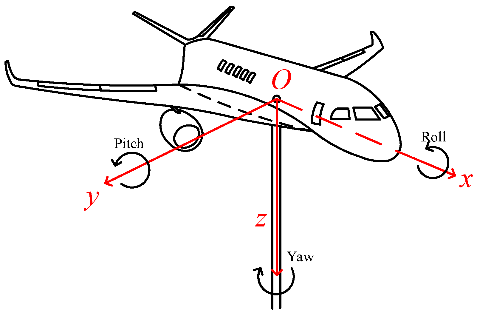
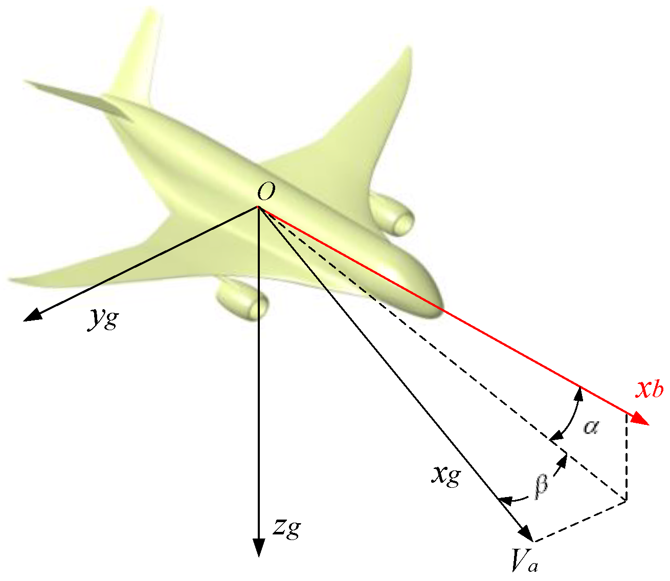
2.1. Flight Dynamics Modelling

Generally, the aircraft is symmetrical about the Oxbzb plane under the body coordinate system, i.e., Ixy = Iyz = 0. The lateral-directional rotation dynamics and kinematic equations of the test model around the centre of mass are the same as free flight, as shown in Equation (1) [23].
{ L = I x p ˙ I x z ( r ˙ + p q ) ( I y I z ) q r N = I z r ˙ I x z ( p ˙ q r ) ( I x I y ) p q ϕ ˙ = p + q sin ϕ tan θ + r cos ϕ tan θ ψ ˙ = q sin ϕ sec θ + r cos ϕ sec θ
where Ix, Iy, and Iz are the inertia of the three axes; Ixz is the cross inertia; p, q, and r are the roll rate, pitch rate and yaw rate, respectively; and L and N are the rolling and yawing moments of the aircraft, respectively.
The lateral-directional dynamics equation describing the centroid of an aircraft in the body coordinate system is shown in Equation (2) [24]:
m ( d v d t + r u p w ) = F y b = 0
where m is the mass of the model; u, v, and w are the components of airspeed in the body coordinate system; and Fy−b is the combined external force on the y-axis of the aircraft under the body coordinate system. Since the model has no translational motion, the combined external force Fy−b = 0.
In the wind tunnel virtual flight test, the external forces on the model include gravity, the triaxial aerodynamic forces, and the force exerted by the support rod on the model. Project all external forces under the body coordinate system, as shown in Equation (3).
[ \ F y b \ ] = [ X Y Z ] + L b g · [ 0 0 m g ] + [ F x F y F z ]
where Lbg is the rotation matrix from the ground coordinate system to the body coordinate system; Fx, Fy, and Fz are the forces of the support rod on the model in the x-, y-, and z-axis directions, respectively; and X, Y, and Z are the aerodynamic forces on the model in the body coordinate system, respectively.
Substituting the combined external force Fy−b of the model in the body coordinate system derived from Equation (3) into Equation (2), the centre-of-mass dynamics equation of the model is obtained as shown in Equation (4).
m ( d v d t + r u p w ) = Y + m g sin ϕ cos θ + F y
The angle of attack and sideslip, which are important variables in wind tunnel tests, are usually measured by vane sensors. A wind vane sensor needs to be installed at the nose of the aircraft, which may lead to a decrease in the accuracy of the airflow angle measurement, due to the interference of the fuselage. In real flight test, it is necessary to install multiple sensors on the fuselage to measure the flow angle of the aircraft [25]. However, in the wind tunnel virtual flight test, they can be directly solved by the three-axis attitude angles ϕ, θ, ψ. Due to the high accuracy of the attitude angle measurement, the angle of attack and sideslip are also solved with high accuracy. According to the definition of the angle of attack and sideslip, their calculation formulas are as follows [26]:
{ α = tan 1 ( w u ) β = sin 1 ( v V )
As shown in Figure 5, define the ground coordinate system with the origin Og at the centre of mass of the model, with Oxg pointing in the direction of wind velocity, Ozg vertically downwards, and Oyg perpendicular to the Oxgzg plane to the right. In the wind tunnel test, assuming that the direction of the incoming flow is constant, the x-axis of the air coordinate system, ground coordinate system, and flight path coordinate system all coincide. Thus, u, v, and w can be solved using the attitude angle and the coordinate system transformation matrix, which, in turn, directly solves for the airflow angles α and β, as shown in Equation (6).
{ [ u v w ] = L b g [ V 0 0 ] = [ a 11 a 12 a 13 a 21 a 22 a 23 a 31 a 32 a 33 ] [ V 0 0 ] a 11 = cos θ cos ψ a 21 = sin ϕ sin θ cos ψ cos ϕ sin ψ a 31 = cos ϕ sin θ cos ψ + sin ϕ sin ψ α = arctan ( w / u ) = arctan ( a 31 / a 11 ) β = arcsin ( v / V ) = arcsin ( a 21 / V )

2.2. Linearization and Decoupling for Equations of Motion

The motion response of the wind tunnel virtual flight for the test model can be decoupled as the superposition of two parts of motion, namely (1) the motion of unconstrained free flight, and (2) the effect on the motion of the model by the force of the support device on the model. Through linearization, the lateral-directional motion equation can be described as the decoupling form of the effects of free flight aerodynamic force, gravity, and supporting force on the model motion.
In the linearization of the equations of motion, the amount of side force, rolling, and yawing moment perturbations, relative to the equilibrium flight motion, can be expressed as linear relationships, with ΔY, ΔL, and ΔN expressed as Equation (7): [24].
{ Δ Y = Y β Δ β + Y r Δ r + Y p Δ p + Y δ r Δ δ r Δ L = L β Δ β + L p Δ p + L r Δ r + L δ a Δ δ a + L δ r Δ δ r Δ N = N β Δ β + N p Δ p + N r Δ r + N δ r Δ δ r
As the displacement of the test model is constrained, the combined force of gravity, aerodynamic forces, and the forces acting on the model by the support device are zero. Making the combined force Fy−b of the model in Equation (3) be 0, the expression of the force acting on the model by the support device Fy can be obtained:
F y = Y m g sin ϕ cos θ
We linearized Equation (8) with a base state parameter of ϕ* = 0°, and the result of the linearization is shown in Equation (9).
Δ F y = Δ Y m g cos θ * Δ ϕ = Y β Δ β Y p Δ p Y r Δ r m g cos θ * Δ ϕ Y δ r Δ δ r
Equation (9) shows that ΔFy can be expressed in the form of a linear superposition of aerodynamic forces and gravity. The linear expression for the force ΔFy acting on the model by the support device can be obtained from Equation (9) as:
Δ F y = F y β Δ β + F y p Δ p + F y r Δ r + F y ϕ Δ ϕ + F y δ r Δ δ r
where Fy−β, Fy−p, Fy−r, Fy−ϕ, and Fy−δr denote the derivatives of the side force generated by the support device in the body coordinate system, with respect to the sideslip angle, roll rate, yaw rate, roll angle, and rudder deflection, respectively; the specific expressions are shown in Equation (11).
{ F y β = Y β F y ϕ = m g cos θ * F y p = Y p F y δ r = Y δ r F y r = Y r
The lateral-directional equations of motion for the wind tunnel virtual flight shown in Equations (1) and (4) are linearised, and the expressions ΔY, ΔL, ΔN, and ΔFy, shown in Equations (7) and (10), are substituted into these linearised equations of motion to obtain the linearization results for the test model at the base state of V* and α*, as shown in Equation (12):
[ Δ β ˙ Δ p ˙ Δ r ˙ Δ ϕ ˙ ] = [ Y ¯ β α * + Y ¯ p Y ¯ r 1 g cos θ * / V * L ¯ β L ¯ p   L ¯ r 0 N ¯ β N ¯ p N ¯ r 0 0 1   tan θ * 0 ] [ Δ β Δ p Δ r Δ ϕ ] + [ 0 Y ¯ δ r L ¯ δ a L ¯ δ r N ¯ δ a N ¯ δ r 0 0 ] [ δ a δ r ] A 1 B 1 + [ Y ¯ β Y ¯ p Y ¯ r g cos θ * / V * 0 0 0 0 0 0 0 0 0 0 0 0 ] [ Δ β Δ p Δ r Δ ϕ ] + [ 0 Y ¯ δ r 0 0 0 0 0 0 ] [ δ a δ r ] A 2 B 2
where A1 and B1 represent the free flight lateral-directional stability matrix and the control matrix of the control surface, respectively, and A2 represents the matrix of the additional motion of the model caused by the support force. In addition, the deflection of the V-tail control surface generates side force and the constraints of the support device have an impact on the control matrix, as shown in B2. The expressions for each lateral-directional dynamic derivative in Equation (12) are shown in Table 2.
To simulate the free flight motion of the aircraft through the results of aerodynamic parameter identification from the wind tunnel virtual flight test, the effects of the A2 and B2 matrices in Equation (12) need to be eliminated. For ease of description, Equation (12) is rewritten into the form shown in Equation (13). The mathematical expressions in the box are the differences in the lateral-directional equations of motion between the wind tunnel virtual flight and the free flight.
[ Δ β ˙ Δ p ˙ Δ r ˙ Δ ϕ ˙ ] = [ Y ¯ β + Y ¯ β α * + Y ¯ p + Y ¯ p Y ¯ r 1 + Y ¯ r g cos θ * V * + g cos θ * V * L ¯ β L ¯ p   L ¯ r 0 N ¯ β N ¯ p N ¯ r 0 0 1   tan θ * 0 ] [ Δ β Δ p Δ r Δ ϕ ] + [ 0 Y ¯ δ r + Y ¯ δ r L ¯ δ a L ¯ δ r N ¯ δ a N ¯ δ r 0 0 ] [ Δ δ a Δ δ r ] A B
The lateral-directional aerodynamic parameter identification model for the wind tunnel virtual flight test can be established according to Equation (13). As the displacement of the model is constrained, it is not possible to identify the side force derivatives of the model directly from the motion of the model; therefore, a step-by-step identification method for the side force derivatives, rolling, and yawing moment derivatives needs to be established.

3. Design Method for Excitation Signals Based on Frequency Domain Analysis

In wind tunnel virtual flight tests, displacement constraints lead to changes in the dynamics of the model, and appropriate excitation signals need to be designed to fully excite the aircraft’s dynamic characteristics, thus ensuring the accuracy of the identification of the lateral-directional aerodynamic derivatives. This paper establishes a method for the selection of excitation signal types and their parameter design based on frequency domain analysis.

3.1. Selection of Excitation Signal Type

The traditional design method of the excitation signal is to solve for the optimal excitation signal by minimizing the deviation or covariance of the aerodynamic parameter identification results [16]. For open-loop controlled aircraft, the above excitation signal design methods are applicable. However, for aircraft with a control augmentation law, since the above signal design method does not consider the feedback effect of the flight control law (as shown in Figure 6), the flight control law may have a significant effect on the excitation signal [4], so it cannot guarantee that the actual maneuvering signal of the aircraft can adequately excite the motion characteristics of the aircraft.
This paper proposes a method for excitation signal type selection based on frequency domain analysis. The most commonly used excitation signals include dipole square wave, 3211-multipole square wave, sine wave, and frequency sweep signals. The dipole square and sine wave signals have a single frequency range and are relatively unsuitable as excitation signals. The 3211-multipole square wave and frequency sweep signals are loaded on the control surface of the test model, and the data before and after the action of the excitation signals are analysed in the time domain and frequency domain to select the signal type that is less influenced by the flight control law.
Taking directional manipulation as an example, by inputting 3211 and frequency sweep excitation signals to the rudder, the waveform changes of the signals are observed after the feedback effect of the flight control law, and the typical results are shown in Figure 7.
As seen from Figure 7, the flight control law has a large effect on the 3211-multipole square wave signal, with a large irregular change in the waveform, while it has a small effect on the frequency sweep signal, with a slight change in frequency. The frequency spectrum of the time-domain changes of the above two types of excitation signals is analysed by fast Fourier transform, and the frequency band changes of the signal energy distribution are observed, as shown in Figure 8.
From Figure 8, it can be seen that after the feedback influence of the flight control law, the spectral shape of the 3211 signal changes significantly and the frequency range of the energy distribution of the signal becomes narrower, while the spectral shape of the frequency sweep signal changes to a relatively small extent and the frequency range of the energy distribution of the signal does not change significantly.
According to the above analysis, when a 3211-multipole square wave is input into the rudder of an aircraft with a closed-loop flight control law, the final rudder signal will have a large degree of irregular change, compared with the initial input excitation signal. However, if the sweep signal is input, the time domain waveform of the signal does not change much, and the frequency band width and position of the signal energy distribution do not change significantly. In addition, the long duration of the sweep signal allows for a continuous input signal to the control surface to excite the desired motion pattern of the aircraft. These laws also apply to the excitation signals of the ailerons. In summary, it is recommended to select the frequency sweep signal as the excitation signal for lateral-directional aerodynamic parameter identification.

3.2. Design of Excitation Signal Parameters

The design parameters of the frequency sweep signal include the low frequency limit ωl, the high frequency limit ωh, and the signal amplitude |A|. In this paper, a method of excitation signal parameter design based on frequency domain analysis is proposed to design the frequency band and amplitude magnitude of the excitation signal. Bode diagram analysis of the equations of motion of the aircraft is carried out to observe the amplitude response of each parameter to be identified with the change in excitation signal frequency. The frequency range of the excitation signal is determined by ensuring that the amplitude response of the aerodynamic forces or moments caused by each motion variable (β, p, r, ϕ), as well as the manipulation variables (δa, δr), is sufficiently large. Finally, the amplitude of the excitation signal is adjusted, so that the signal has high energy in the designed frequency band.
Equation (14) is the observation equation for the lateral-directional motion of the aircraft, which contains the observation equations for the side force, rolling moment, and yawing moment. The Bode diagram analysis of the lateral-directional equations of motion shown in Equation (13) is carried out to observe the amplitude response of the component of side force, rolling moment, and yawing moment in Equation (14), with a change of rudder and aileron frequency.
{ Δ Y = Y β Δ β + Y r Δ r + Y δ r Δ δ r Δ p ˙ = L ¯ β Δ β + L ¯ p Δ p + L ¯ r Δ r + L ¯ δ a Δ δ a + L ¯ δ r Δ δ r Δ r ˙ = N ¯ β Δ β + N ¯ p Δ p + N ¯ r Δ r + N ¯ δ r Δ δ r
Taking directional manipulation as an example, the magnitude response curves N β Δ β ( ω ) / δ r , N p Δ p ( ω ) / δ r , N r Δ r ( ω ) / δ r , and N δ r Δ δ r ( ω ) / δ r of N β Δβ, N p Δp, N r Δr and N δ r Δ δ r with the change in rudder frequency are drawn according to the yawing moment observation equation shown in Equation (14). The amplitude response curves L β Δ β ( ω ) / δ r , L p Δ p ( ω ) / δ r , L r Δ r ( ω ) / δ r , and L δ r Δ δ r ( ω ) / δ r of L β Δ β , L p Δ p , L r Δ r , and L δ r Δ δ r with the change in rudder frequency are drawn according to the rolling moment equation, drawing the amplitude response curves |YβΔβ(ω)/δr|, |YrΔr(ω)/δr|, and |YδrΔδr(ω)/δr| of YβΔβ, YrΔr, and YδrΔδr with the variation of rudder frequency according to the side force equation.
Figure 9 shows the amplitude response curves of each yawing moment component with the change in rudder frequency. In the same way, the amplitude–frequency characteristic curves of the rolling moment and side force components with the frequency of the excitation signal can be obtained. The frequency corresponding to the peak of the resonance is approximately equal to the Dutch roll mode frequency of the aircraft. When the excitation signal frequency is lower or higher than a certain range, the response amplitude of each yawing moment component decreases, and the identification accuracy of all yawing moment derivatives decreases.
To ensure the identifiability of each yawing moment derivative, the magnitude-frequency response magnitudes of the yawing moment components N β Δ β , N r Δ r , N p Δ p , and N δ r Δ δ r caused by the sideslip change Δβ, yaw rate change Δr, roll rate change Δp, and rudder deflection Δδr should not differ significantly. The time domain curves of each yawing moment component, with different frequencies of rudder signal inputs, are given in Figure 10.
In Figure 10a, when the excitation signal frequency is too low, the response of the angular acceleration of the yaw angle Δ r ˙ is almost zero. In this case, the static stability moment generated by N β Δ β and the manipulation moment generated by N δ r Δ δ r almost cancel each other out, resulting in a small yawing moment, which makes it difficult to excite the yaw rate response; therefore, it is not possible to accurately identify all the yawing moment derivatives. In Figure 10c, when the excitation signal frequency is too high, the aircraft response is much slower than the manipulation speed, resulting in small changes in the yaw rate, roll rate, and sideslip, leading to small response amplitudes in N β Δ β , N p Δp, and N r Δ r . Therefore, all yawing moment derivatives cannot be accurately identified. In Figure 10b, when the excitation signal frequency is appropriate, the amplitude response of all yawing moment components are on the same order of magnitude, and the identification results will be accurate. In summary, to ensure the identification accuracy, the excitation signal must be in a certain frequency range.
In the same way, for the rolling moment observation equation shown in Equation (14), the magnitude response magnitudes of the rolling moment components L β Δ β , L r Δ r , L p Δ p , and L δ r Δ δ r caused by the sideslip, yaw rate, roll rate, and rudder surface deflection should not differ significantly. The magnitude response magnitudes of each side force component YβΔβ, YrΔr, and YδrΔδr in the side force observation equation should not differ significantly.
In page 44 of reference [27], it is stated that, when the component of a certain aerodynamic force or moment occupies at least 10% of the maximum aerodynamic force or moment component, the aerodynamic derivative corresponding to the component is considered to be identifiable. To further improve the accuracy of the identification results, a more stringent requirement is used, i.e., when the component of an aerodynamic force or moment accounts for at least 10% of the full aircraft aerodynamic force or moment, the aerodynamic derivative corresponding to that component is considered identifiable. Therefore, the sum of the response amplitude of each aerodynamic force and moment component at all frequencies is calculated in the Bode diagram, and the value corresponding to the total response amplitude 1/10 is calculated, as shown in Equation (15).
{ | A | C n ω i = 1 10 ω i ( | A | N ¯ β Δ β + | A | N ¯ p Δ p + | A | N ¯ r Δ r + | A | N ¯ δ r Δ δ r ) | A | C l ω i = 1 10 ω i ( | A | L ¯ β Δ β + | A | L ¯ p Δ p + | A | L ¯ r Δ r + | A | L ¯ δ r Δ δ r ) | A | C Y ω i = 1 10 ω i ( | A | Y β Δ β + | A | Y δ r Δ δ r + | A | Y r Δ r )
where | A | N β Δ β , | A | N p Δ p , | A | N r Δ r , and | A | N δ r Δ δ r are the response amplitudes of each yawing moment component when the rudder signal frequency is ωi; | A | L β Δ β , | A | L p Δ p , | A | L r Δ r , and | A | L δ r Δ δ r are the response amplitudes of each component of the rolling moment; and | A | Y β Δ β , | A | Y δ r Δ δ r , and | A | Y r Δ r are the response amplitudes of each side force component. | A | C n ω i , | A | C l ω i , and | A | C Y ω i are 1/10 of the total response amplitudes of the yawing moment, rolling moment, and side force at a rudder signal frequency of ωi, respectively.
According to Equation (15), 1/10 of the total response amplitudes of the yawing moment, rolling moment and side force at different rudder frequencies can be calculated and connected to a curve. The dashed line in Figure 9 is the demarcation line corresponding to 1/10 of the total response amplitude of the yawing moment, which is defined as the identifiable boundary of yawing moment derivatives corresponding to different rudder frequencies. Using the same method, identifiable boundaries for the rolling moment, as well as the side force derivatives, can also be obtained.
When the response amplitude of a force or moment corresponding to an aerodynamic derivative is above the identifiable boundary, it means that the derivative is identifiable at this frequency; otherwise, it is not. When the frequency of the rudder signal is in the range ωδr·Cn [ω1~ω2] in Figure 9, i.e., the amplitude responses of all yawing moment components are above the identifiable boundary, all yawing moment derivatives are identifiable. Therefore, the frequency band of the rudder excitation signal determined by the yawing moment derivatives is in the range of ωδr·Cn. The same method can be used to obtain the frequency band range of the rudder excitation signal determined by rolling moment, as well as side force derivatives, such as ωδr·Cl and ωδr·CY. To ensure that all lateral-directional aerodynamic derivatives are identifiable, it is necessary to take the intersection of ωδr·Cn, ωδr·Cl, and ωδr·CY to obtain the frequency band of the rudder excitation signal ωδr.
ω δ r = ω δ r C n ω δ r C Y ω δ r C l
In the same way, the frequency band of the aileron excitation signal ωδa can be obtained.
ω δ a = ω δ a C n ω δ a C Y ω δ a C l
where ωδa·Cn, ωδa·Cl, and ωδa·CY are the frequency band ranges of the aileron signals determined by the yawing moment, rolling moment, and side force derivatives, respectively.
The amplitude of the aileron and rudder signals need to be within the appropriate range. A large excitation signal amplitude will lead to a large change in the aircraft sideslip angle, thus introducing nonlinear aerodynamic effects; if the signal amplitude is too small, it will not be easy to excite the aircraft’s lateral-directional motion mode. Therefore, first, it is necessary to ensure that the variation in the aircraft sideslip angle is approximately ±2° to ensure that the aerodynamic derivatives are in the linear segment. Then, the amplitude of the excitation signal is determined according to the requirement of the change in sideslip angle under the consideration of the feedback effect of the flight control law.

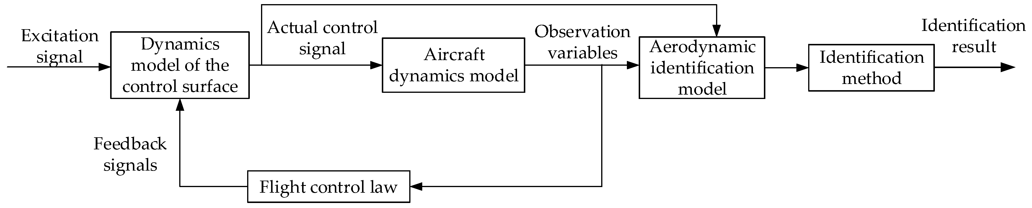
4. Step-by-Step Identification Method for the Aerodynamic Parameters

4.1. Identification Method of Side Force Derivatives

In the wind tunnel virtual flight test, the position of the test model is fixed, and the combined external force of the whole aircraft is zero, so the side force derivatives of the model cannot be directly identified by the motion of the model. However, the test model has a strain gauge balance installed at the centre of mass to measure the side force of the whole aircraft in real time, so the measured value of the side force Ym can be used as an observed variable to identify side force derivatives. The identification model of side force derivatives is shown in Equation (18).
Y m = Y β Δ β + Y p Δ p + Y r Δ r + Y δ r Δ δ r
where Ym is the side force of the whole test model directly measured by the force balance; Δβ, Δp, Δr, and Δδr are the amount of change in sideslip angle, roll rate, yaw rate, and V-tail control surface, which can be measured directly by the sensors. The parameter to be identified is Θ = [Yβ, Yp, Yr, Yδr].
Since the side force measured by the force balance is the actual aerodynamic force on the model without the force of the support device, the identification results based on the measured data are the side force derivatives of free flight.
For the side force observation equation shown in Equation (18), the side force derivatives can be directly identified using the least squares method. The general form of least squares identification is shown in Equation (19) [28]:
{ y = X Θ z = X Θ + v
where Θ is a vector composed of the aerodynamic derivatives to be identified; y is the aerodynamic force of the theoretical output from the test model, i.e., the side force; z is the side force actually measured by the force balance; X is the matrix of independent variables composed of parameters, such as the motion variables (β, p, r, ϕ) and manipulation variables (δa, δr) of the aircraft; and v is the measurement noise matrix. In the wind tunnel test, the measurement accuracy of the strain balance is high, and v can be regarded as white noise with a mean value of 0, as shown in Equation (20):
E ( v ) = 0 E ( v v T ) = σ 2 I
The least squares solutions of the aerodynamic lift and drag derivatives to be identified are:
Θ ^ = ( X T X ) 1 X T z
Yβ, Yp, Yr, and Yδr are identified by the least square method and substituted into Table 2 to solve the aerodynamic derivatives C, Cyp, Cyr, and Cyδr.

4.2. Identification Method of Rolling and Yawing Moment Derivatives

Selecting β, p, r, and ϕ as the state variables for the lateral-directional aerodynamic parameter identification, the state equation of the lateral-directional aerodynamic parameter identification model for wind tunnel virtual flight is shown in Equation (22) [16].
{ p ˙ = ( c 1 r + c 2 p ) q + c 3 L + c 4 N r ˙ = ( c 5 p c 2 r ) q + c 4 L + c 6 N ϕ ˙ = p + tan θ ( q sin ϕ + r cos ϕ ) β ˙ = r cos α + p sin α
In Equation (22), the expressions of rolling and yawing moments L and N are shown in Equation (7), and the expressions of c1, c2, c3, c4, c5, and c6 are shown in Equation (23). The lateral-directional moment derivatives to be identified are Θ = [Lβ, Lp, Lr, Lδa, Lδr, Nβ, Np, Nr, Nδr].
{ c 1 = ( I y I z ) I z I x z 2 I x I z I x z 2 c 4 = I x z I x I z I x z 2 c 2 = ( I x I y + I z ) I x z I x I z I x z 2 c 5 = I x ( I x I y ) I x z 2 I x I z I x z 2 c 3 = I z I x I z I x z 2 c 6 = I x I x I z I x z 2
pm, rm, βm, and ϕm measured by the experiment are chosen as the observation variables, so the observation equation is shown in Equation (24).
{ p m = p + v p r m = r + v r β m = β + v β ϕ m = ϕ + v ϕ
where p, r, β, and ϕ are theoretical outputs and vp, vr, vβ, and vϕ are measurement noise. Aerodynamic derivatives of the test model can be obtained by identifying aerodynamic parameters of the nonlinear motion model shown in Equations (22)–(24). The most widely used method is the output error method based on maximum likelihood estimation [29]. General nonlinear dynamic equations can be expressed in the form shown in Equation (25):
{ x ˙ ( t ) = f [ x ( t ) , u ( t ) , Θ ] x ( t 0 ) = x 0 y ( t ) = g [ x ( t ) , u ( t ) , Θ ] z ( t k ) = y ( t k ) + v ( t k )
where x is the state variable (p, r, β, ϕ); u is the input variable (δa, δa); y is the output variable (p, r, β, ϕ); z is the observed variable (pm, rm, βm, ϕm); f and g are the general nonlinear functions; and Θ is the parameter to be identified. Assume that the measurement noise v is Gaussian white noise with zero mean and a covariance matrix of R.
The output error method based on the maximum likelihood method is used to estimate the aerodynamic derivatives to be identified in Equations (22)–(24). The optimization function and iterative algorithm are shown in Equations (26) and (27).
J ( Θ , R ) = 1 2 k = 1 N [ z ( t k ) y ( t k ) ] T R 1 [ z ( t k ) y ( t k ) ] + N 2 I n | R |
Starting from the specified initial value Θ0, the Gauss–Newton solution algorithm shown in Equation (27) is used to iterate to find the optimal parameters to be identified [29].
{ Θ i + 1 = Θ i + Δ Θ Δ Θ = k = 1 N [ y ( t k ) Θ ] T R 1 [ z ( t k ) y ( t k ) ] k = 1 N [ y ( t k ) Θ ] T R 1 [ y ( t k ) Θ ]

5. Verification of Identification Results Based on the Wind Tunnel Virtual Flight Test

In conclusion, the lateral-directional aerodynamic parameter identification method of the test model based on wind tunnel virtual flight is formed. The specific identification process is shown in Figure 11. First, the lateral-directional flight dynamics equations of wind tunnel virtual flight are established, and the equations of motion are linearised and decoupled to analyse the differences between the lateral-directional motion equations of wind tunnel virtual flight and free flight, so as to establish the identification model. Second, the amplitude–frequency characteristics for the equations of motion are analysed to determine the type of excitation signal, and the frequency range and amplitude of the aileron and rudder signals based on the identifiability requirements of the aerodynamic derivatives. Third, the least squares method is used to identify the side force derivatives of the wind tunnel virtual flight test, which can measure the aerodynamic force of the whole aircraft in real time through the force balance. Based on the equations of motion for wind tunnel virtual flight, the identification of rolling and yawing moment derivatives is completed by maximum likelihood estimation. Finally, the verification of the identification results is completed.

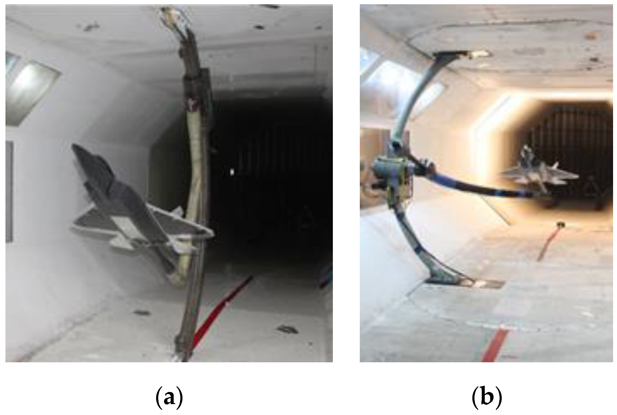
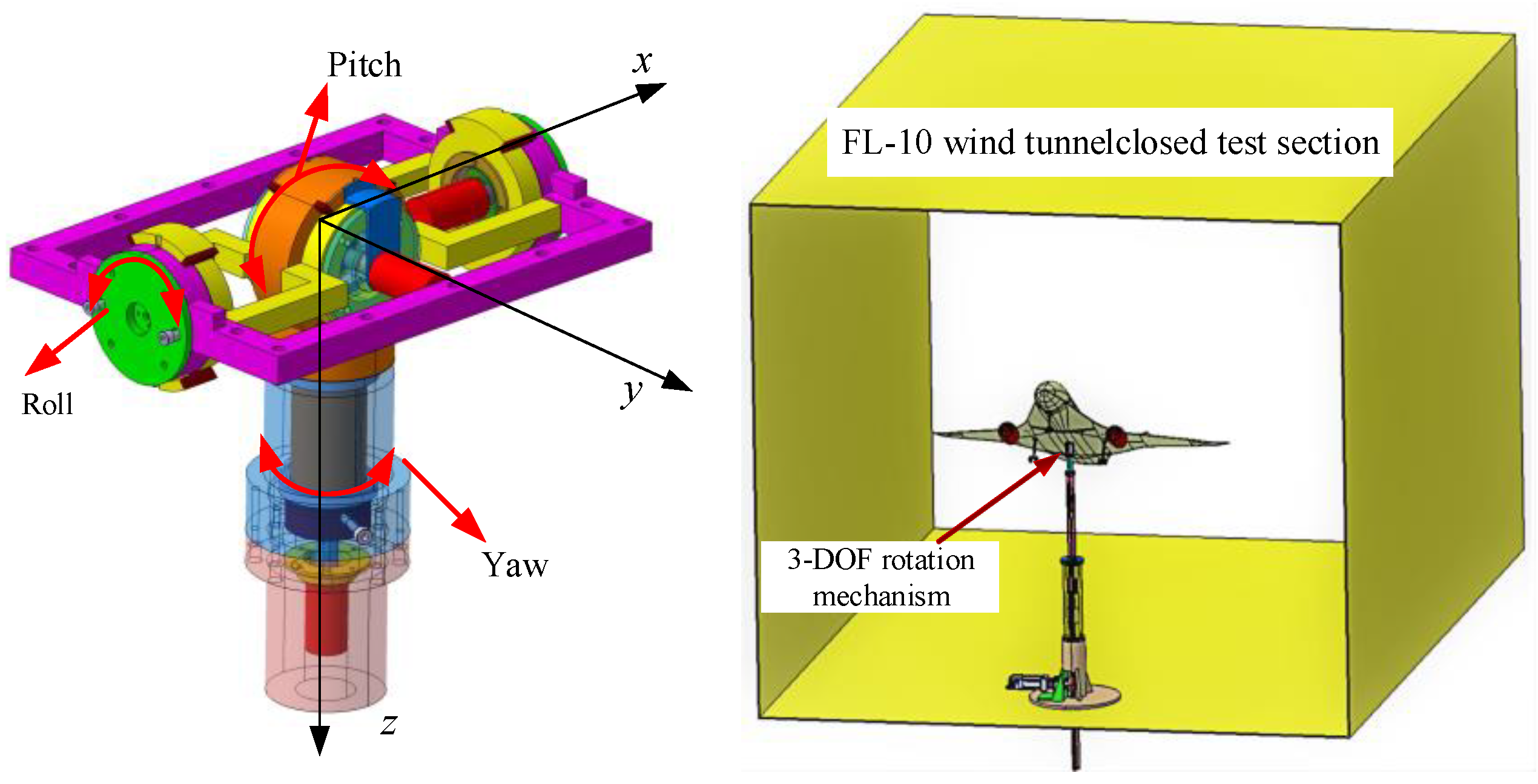
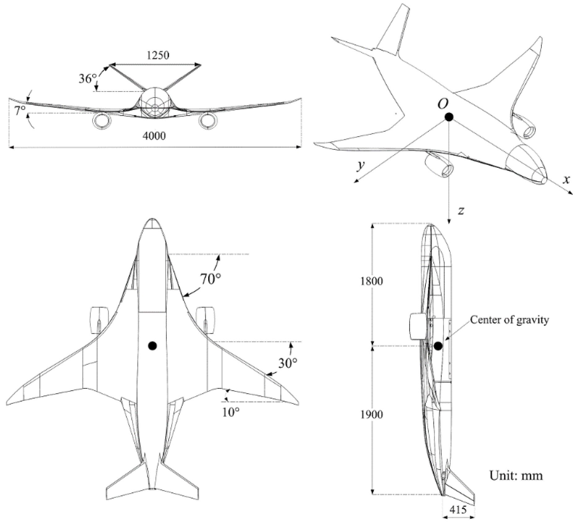
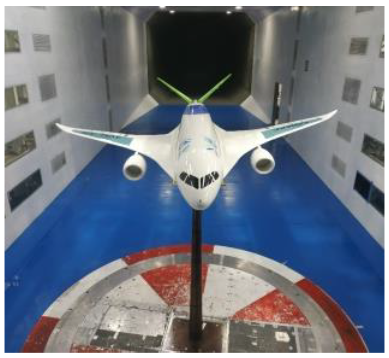
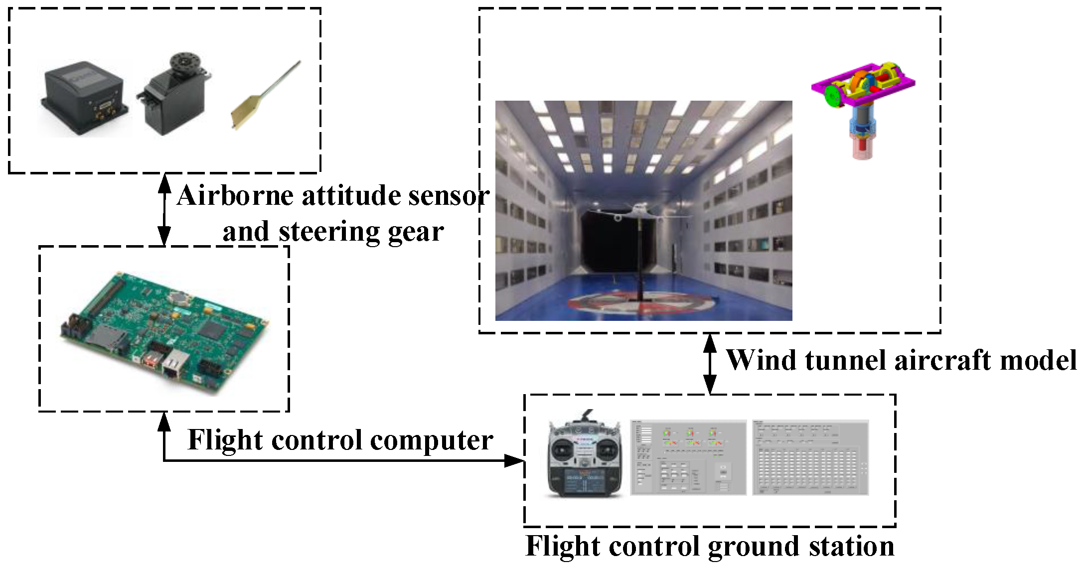
5.1. Facility for Wind Tunnel Virtual Flight Tests

The wind tunnel virtual flight test was carried out in a FL-10 wind tunnel at the AVIC Aerodynamics Research Institute [30]. As shown in Figure 12, the test model is installed in the closed test section of the wind tunnel, the size of which is 8 m × 6 m, and the maximum wind speed of the wind tunnel is 110 m/s. The test model scaling ratio k = 1/9 and the design parameters of the test model can be obtained according to the similarity criterion between the full-size aircraft and the scaled-model [31,32], as shown in Table 3.
The flight test control and measurement system are shown in Figure 13. The aircraft model is equipped with attitude measurement sensors, wind vane sensors, rotary encoders, flight control computers, and servos. The IMU attitude sensor is used to measure the three-axis attitude angle and angular velocity of the model; the wind vane sensor is used to measure the angle of attack and sideslip angle of the model; the rotary encoder is used to measure the deflection angle of the rudder surface; and servos drive the deflection of the control surfaces. The flight control computer collects data from the on-board sensors and runs control law algorithms to control the attitude and altitude of the test model through the control surfaces. In addition, the ground station is developed and designed based on the LabVIEW software platform, which can display the data during the wind tunnel virtual flight test in real time.
The lateral-directional control law structure of the model is shown in Figure 14. The direction of the roll axis adopts the roll angle command configuration ϕcmd, and the direction of the yaw axis is controlled by the sideslip angle command βcmd.
The speeds V = 30 m/s and α = 6° are chosen as the initial trim flight state for the wind tunnel test, and the lateral-directional control law parameters of the test model are Kp = 0.25, KP−ϕ = 2.18, KI−ϕ = 0.14, Kβ = 0.63, Kr = 0.37, KP−β = 0.10, KI−β = 0.50, and Kari = 0.33.

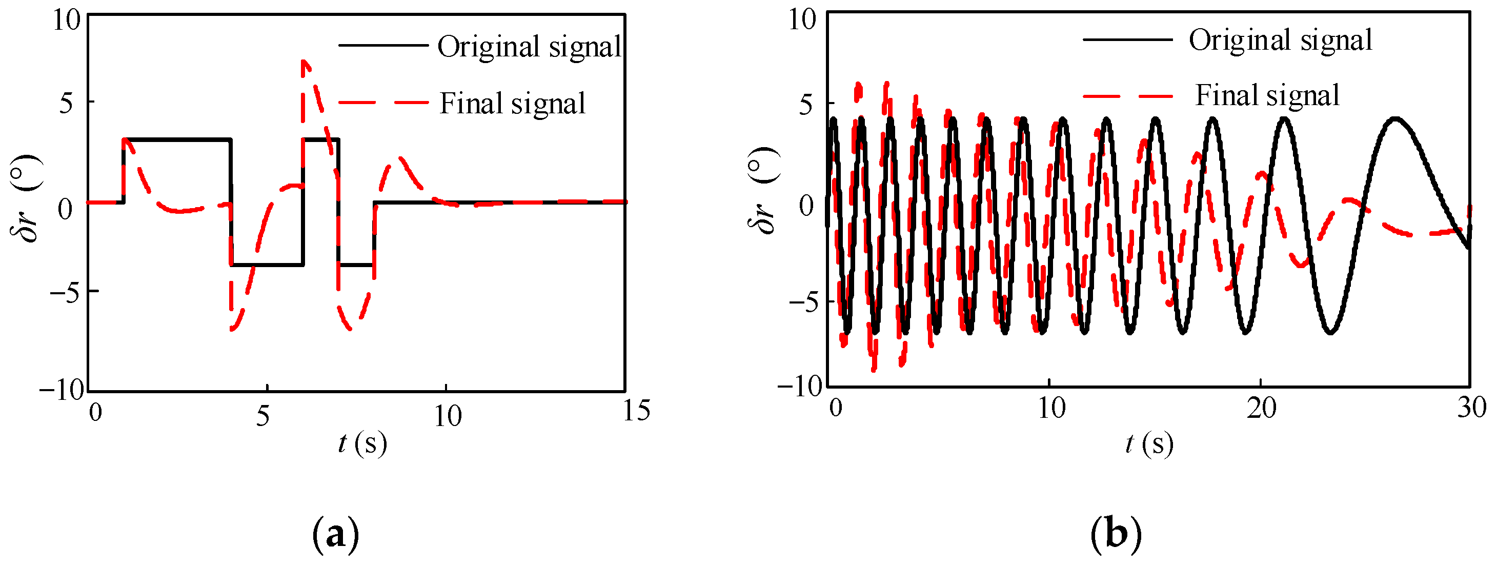
5.2. Design of the Excitation Signal

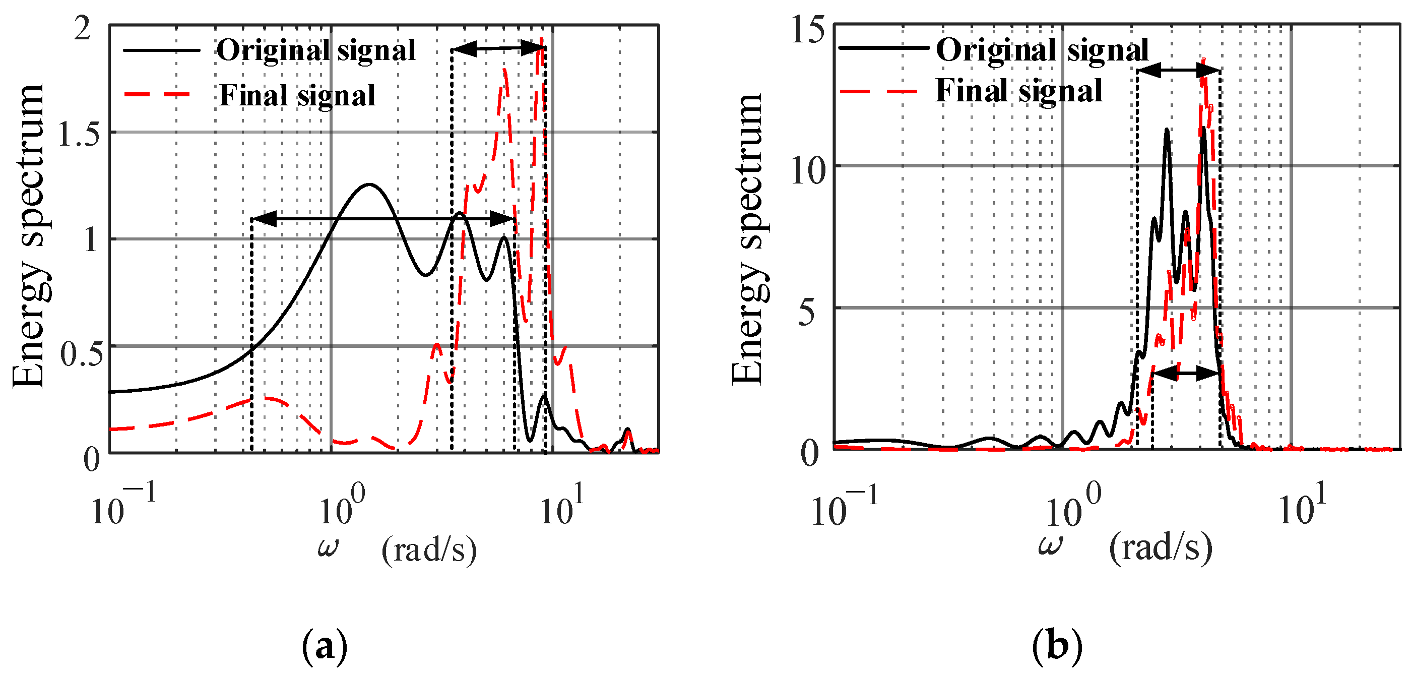
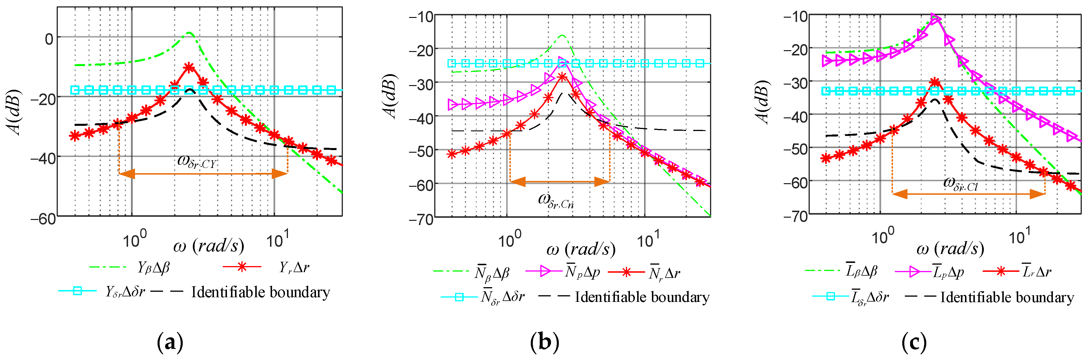
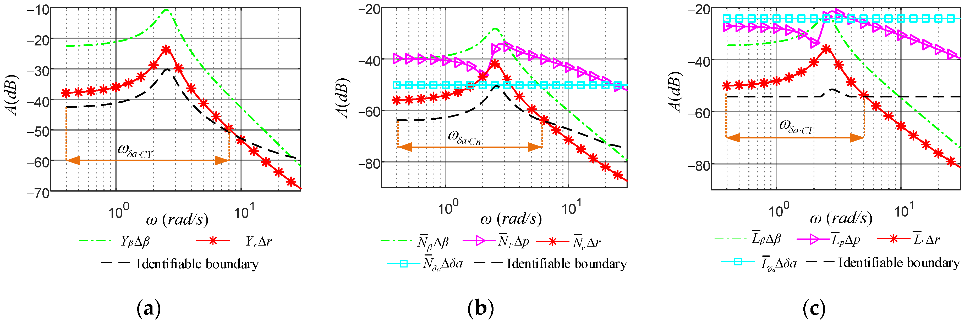
5.2.1. Determination of the Rudder and Aileron Frequency Range

According to the analysis in Section 3.1, the frequency sweep signal is selected as the input signal for the rudder, as well as the aileron. The lateral-directional motion of the model is shown in Equations (18) and (22) are established based on the prior aerodynamic data of the test model. The amplitude–frequency response curves of the side force, yawing moment, and rolling moment components varying with the frequency of the rudder and aileron are shown in Figure 15 and Figure 16, respectively.
The Dutch roll mode frequency of the test model at V = 30 m/s and α = 6° flight state is approximately 2.5 rad/s. The resonance peaks of the amplitude–frequency characteristic curves of the aerodynamic parameters in Figure 15 and Figure 16 are approximately equal to the Dutch roll mode frequency. The frequency band ranges of the rudder excitation signals determined by the yawing moment, rolling moment, and side force aerodynamic derivatives determined by the method presented in Section 3 are ωδr·Cn = [1.1, 5.3] rad/s, ωδr·Cl = [0.7, 8.7] rad/s, and ωδr·CY = [0.8, 12.0] rad/s, respectively. Taking the intersection of ωδr·Cn, ωδr·Cl, and ωδr·CY, the band range of the rudder excitation signal is obtained as ωδr = ωδr·Cn ωδr·CY ωδr·Cl = [1.1, 5.3] rad/s. In the same way, the band range of the aileron excitation signal can be obtained as ωδa = ωδa·Cn ωδa·CY ωδa·Cl = [1.2, 5.2] rad/s.
In summary, to ensure the identifiability of the lateral-directional aerodynamic derivatives of the test model, the optimal frequency range for the rudder, as well as the aileron frequency sweep excitation signals, is ωδr = [1.1, 5.3] rad/s and ωδa = [1.2, 5.2] rad/s, approximately between 0.5 and 2 times the Dutch roll modal frequency.

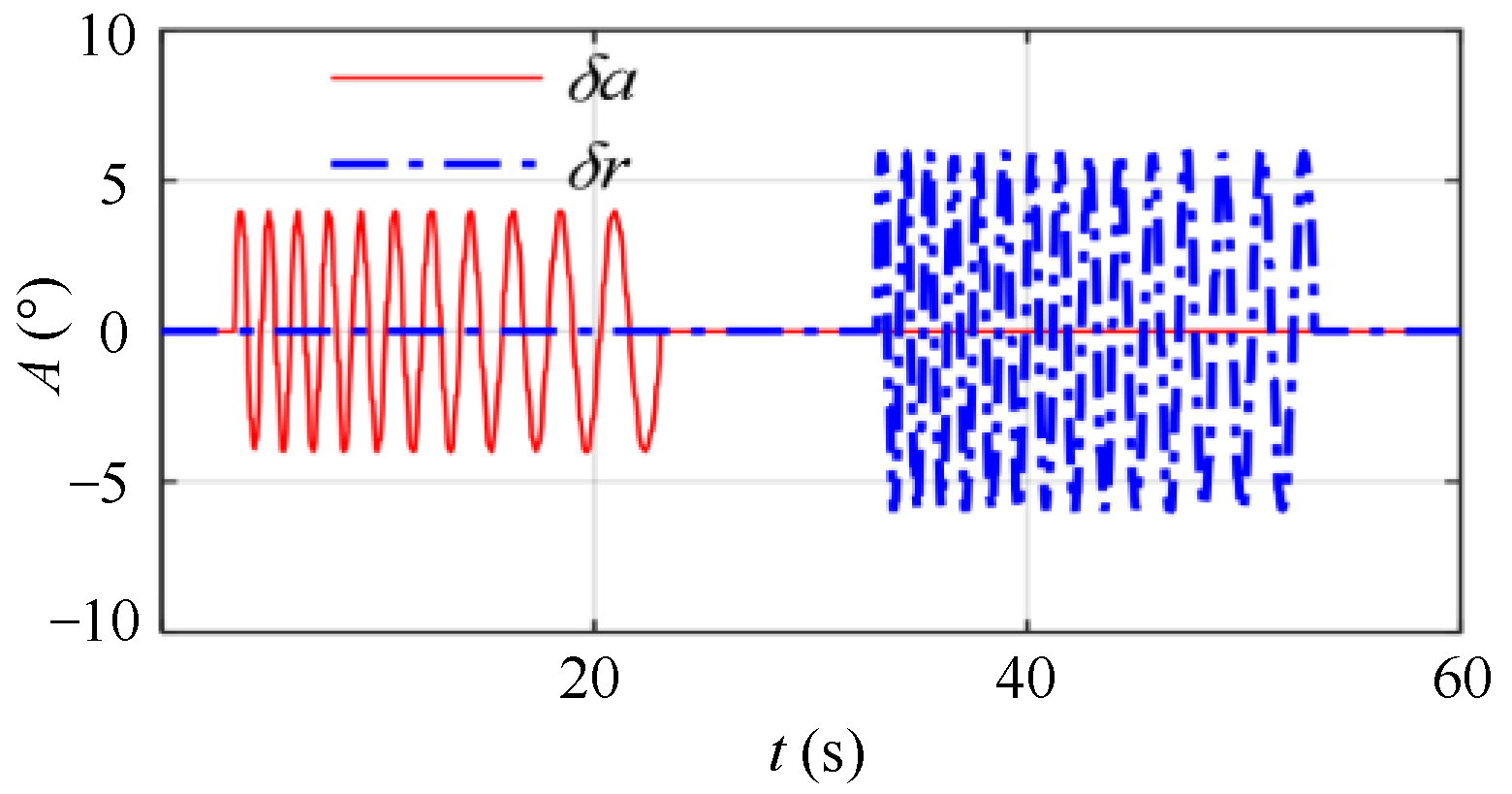
5.2.2. Determination of the Signal Amplitude

The frequency range of the aileron and rudder frequency sweep signal is selected as ωδa = ωδr = 1.5~5 rad/s in this experiment. To make the sideslip of the test model change within the range of ±2°, the amplitude of the aileron excitation signal is set to 6°, and that of the rudder excitation signal is set to 4°. The lateral-directional excitation signal is shown in Figure 17.

5.3. Identification Results of Aerodynamic Derivatives

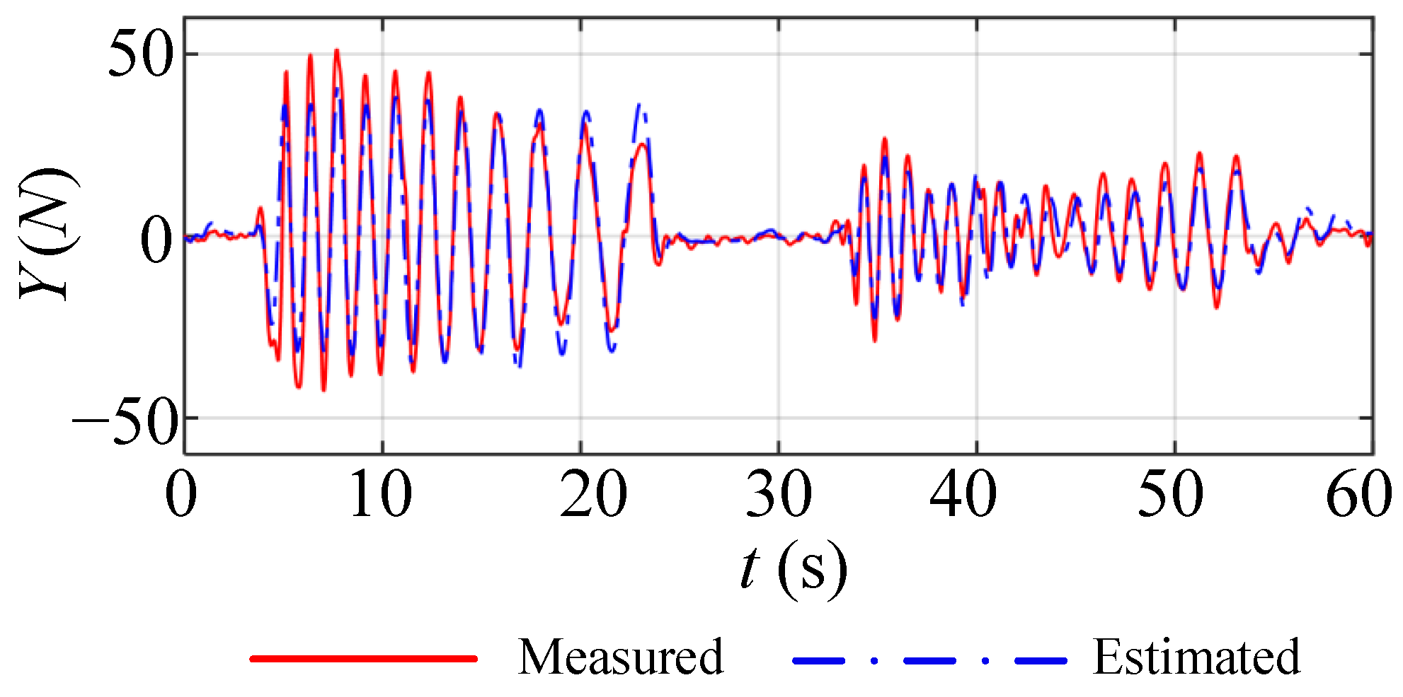
5.3.1. Identification of Side Force Derivatives

The wind tunnel virtual flight test is carried out under the conditions of V = 30 m/s, α = 6°, β = 0°, and δe = −5.6°. The outer ring of the flight control law is the instruction of 0° sideslip angle and 0° roll angle. The excitation signal is directly input on the V-tail control surface and aileron on both sides, and the side force Ym of the test model is measured in real time through the force balance.
The side force Ym, sideslip angle Δβm, yaw rate Δrm, roll rate Δpm, and V-tail control surface deflection angle Δδr of the model measured in the test are substituted into Equation (19), and the side force derivatives of the model are identified by the least squares method, shown in Equation (21). The identification results are shown in Table 4, with the first column of the table showing the aerodynamic derivatives measured in the traditional wind tunnel test. Comparing the identification results with the conventional wind tunnel measurements, it can be seen that the identification results of side force derivatives are close to the reference values, and the deviations are within 10%.
The identification results of the side force derivatives are substituted into Equation (18) to establish the side force observation model of the wind tunnel virtual flight test. Given the excitation signals used in the wind tunnel virtual flight test, the simulation results of the side force observation model, established based on the identification results, are compared with the side force data measured by the test, as shown in Figure 18. The simulation results of the identification model are in high agreement with the data measured by the wind tunnel virtual flight test, and the maximum errors of the side force curves are within 5%.

5.3.2. Identification of Rolling and Yawing Moment Derivatives

The measured angle of attack, sideslip angle, three-axis attitude angle, and three-axis angular rate are taken into the maximum likelihood solution equations shown in Equations (25) and (26) to identify the rolling and yawing moment derivatives of the model, and the identification results are shown in Table 4.
It is to be highlighted that the results for side-force came from least squares (i.e., equation-error method), whereas the results for yawing and rolling moment were obtained via output error method (using the maximum likelihood principle).
According to Table 4, the deviation between the identification results of the yawing and rolling moment derivatives and the conventional wind tunnel measurements is within 10%. The identification results of the rolling and yawing moment derivatives are substituted into Equation (22) to obtain the lateral-directional motion model for the wind tunnel virtual flight test. Given the rudder and aileron excitation signals used in the test, the simulation results of the identified model are compared with the corresponding test data, as shown in Figure 19. The motion response of the identified model is basically consistent with the data of the wind tunnel virtual flight test, and the maximum deviation of all motion parameters is within 5%.
Goodness of fit (GOF) is used to evaluate the consistency between the lateral-directional motion response of the identified model and the wind tunnel virtual flight test data. The GOF formula is shown in Equation (28), where zi is the experimental measurement, z is the mean value of the observed data, and yi is the theoretical output; a GOF value close to 1 indicates that the two sets of data fit well [33].
G O F i = 1 ( z i y i ) T ( z i y i ) ( z i z ¯ ) T ( z i z ¯ )
The GOF between the lateral-directional motion response of the identification model and the wind tunnel virtual flight test is shown in Table 5. The GOF of all motion variables are greater than 0.95. It is proven that the lateral-directional motion response of the identified model is consistent with the wind tunnel virtual flight test data.
In summary, the step-by-step identification method of lateral-directional aerodynamic derivatives introduced in this paper can obtain accurate identification results, and the deviation of all the aerodynamic derivatives from the conventional wind tunnel measurements is within 10%.

5.4. Verification of the Modified Identification Model

By substituting the aerodynamic derivatives identified in Table 4 into the A1 and B1 matrices in Equation (12) and eliminating the A2 and B2 matrices generated by the influence of the support device, a modified lateral-directional motion model for wind tunnel virtual flight can be constructed, as shown in Equation (29).
[ β ˙ p ˙ r ˙ ϕ ˙ ] = [ - 0 . 33 0 . 12 - 0 . 96 0 . 32 - 32 . 60 - 5 . 51 1 . 51 0 4 . 22 - 0 . 32 - 0 . 42 0 0 1 0 . 11 0 ] [ Δ β Δ p Δ r Δ ϕ ] + [ 0 0 . 10 - 19 . 48 7 . 04 - 0 . 17 - 4 . 46 0 0 ] [ δ a δ r ]
V = 30 m/s and α = 6° are selected as the steady flight state of the test model. The 3211-multipole square waves are input to the V-tail control surface, while the other control surfaces are kept fixed. Comparing the simulation results of the identified model of wind tunnel virtual flight before and after the correction with the simulation data of the free flight motion model, the results are shown in Figure 20. The motion models for both wind tunnel virtual flight and free flight are linearised motion models. It should be clarified that the free flight motion model is based on the results of traditional wind tunnel test force measurements, and the correction of the wind tunnel virtual flight motion model is obtained by eliminating the influence of the test rig.
The goodness-of-fit (GOF) is shown in Table 6, comparing the responses of the identified model before and after the correction with the free flight simulation results.
As shown in Figure 20, the response of the modified identification model for wind tunnel virtual flight is in high agreement with the simulation results of the lateral-directional motion of free flight. A small phase shift between the modified wind tunnel virtual flight motion response and the free flight motion response can be seen in Figure 20, but we believe that this small difference can be neglected. Since the motion models of both wind tunnel virtual flight and free flight are linearised motion models, the inaccuracy of the linearised motion models may lead to small differences in the responses of the two. The GOF of each motion data of the identified model before the correction is less than 0.85, while the GOF of each motion data of the model after the correction is greater than 0.95.
In summary, compared with the original wind tunnel virtual flight motion model, the modified motion of the model matches better with the motion of the free flight model, indicating that the modified model can more accurately characterise the lateral-directional motion of the aircraft in free flight.

6. Conclusions

(1)
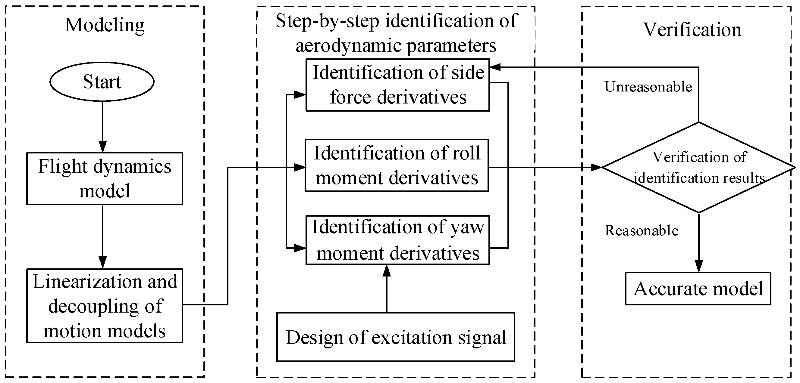
The lateral-directional flight dynamics equations of the wind tunnel virtual flight test model are established. By linearizing the equations of motion to describe the wind tunnel virtual flight test as a decoupled form of the effects of free flight aerodynamic forces and support forces on the model motion, the differences between the lateral-directional dynamics of wind tunnel virtual flight and free flight can be analysed more intuitively, thus establishing a model for the identification of aerodynamic parameters.
(2)
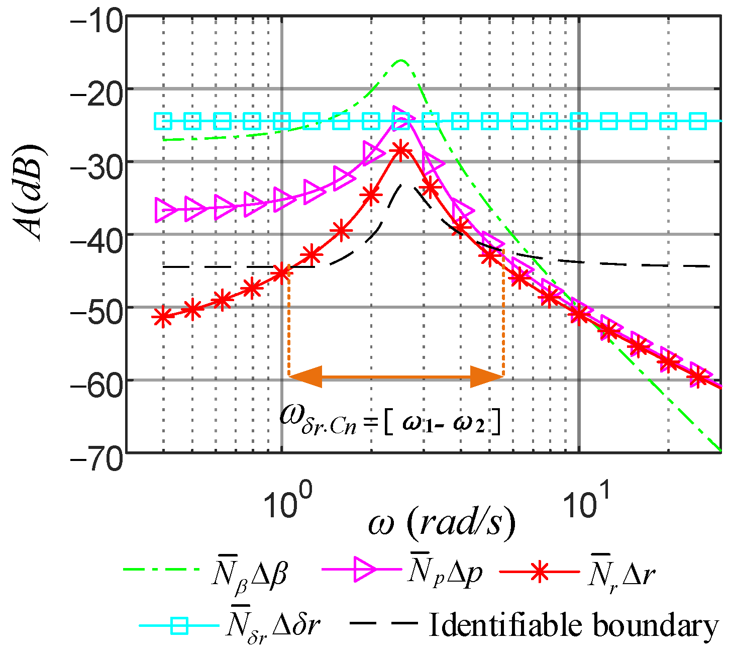
Based on the identifiable requirements of aerodynamic derivatives, the amplitude–frequency characteristics of the equations of motion are analysed to establish the type selection and parameter design method of the lateral-directional excitation signal. The frequency of the lateral-directional excitation signal needs to be between 0.5–2 times the frequency of the Dutch roll mode. Therefore, a suitable actuator needs to be selected for different flight states, so that the deflection rate of the control surface is fast enough. In addition, to identify the aerodynamic model at high angle of attack or high sideslip, it is necessary to design appropriate flight control law to ensure the stability of the test model.
(3)
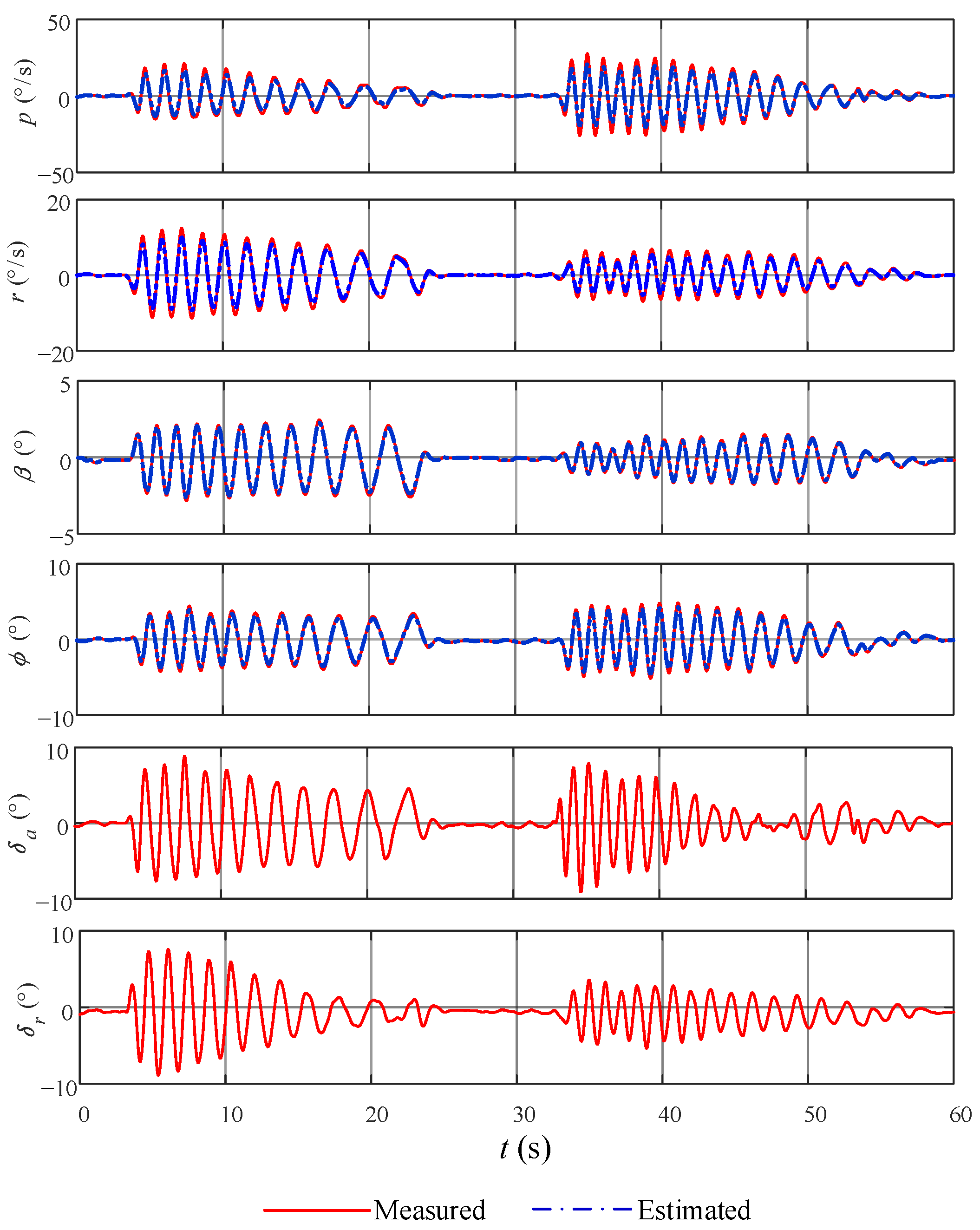
In this paper, a step-by-step method for the identification of side force, rolling, and yawing moment derivatives is established. The identification of the side force derivatives can be achieved by measuring the aerodynamic force of the test model with a force balance. The differences between the identification results of the aerodynamic derivatives and the conventional wind tunnel measurements are within 10%. The lateral-directional motion response of the identified model is basically consistent with the wind tunnel virtual flight test data, and the GOF of all motion variables are greater than 0.95.
(4)
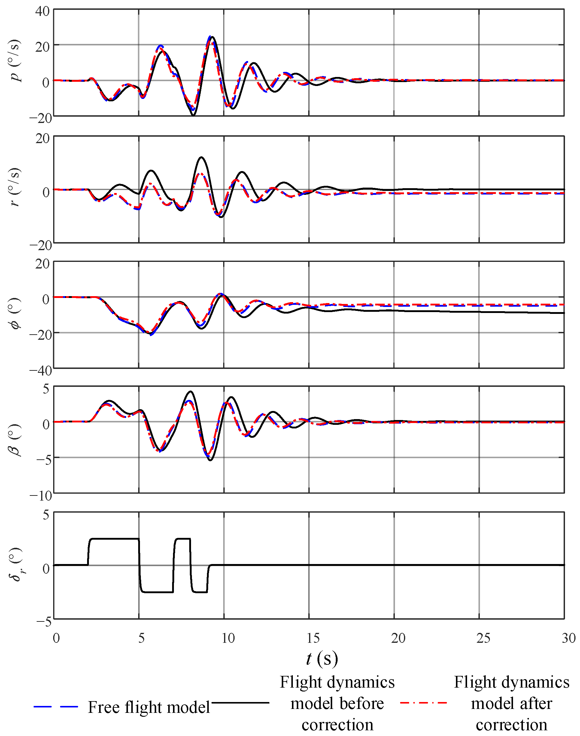
The modified identification model can well-simulate the lateral-directional motion of the conventional wind tunnel test model, and the goodness-of-fit is higher than 0.95, which verifies the correctness of the proposed method.
The proposed method of identifying the lateral-directional aerodynamic parameters of aircraft based on wind tunnel virtual flight tests is simple in principle, and the identification results are highly accurate. The wind tunnel virtual flight test enables the accurate identification of the lateral-directional aerodynamic model at an early stage of aircraft design, which can be compared and corrected with the force measurement results of conventional wind tunnel tests. The proposed method has outstanding advantages in shortening the development cycle of aircraft and reducing risks and costs, but the application of the proposed method to the parameter identification of rotorcraft or spacecraft needs further study.

Author Contributions

Conceptualization, L.W. and S.T.; methodology, L.W.; software, S.T. and S.L.; validation, T.Y., S.T. and Y.W.; formal analysis, C.B.; investigation, L.W.; resources, Y.W.; data curation, C.B.; writing—original draft preparation, S.T., T.Y. and S.L.; writing—review and editing, L.W., C.B. and Y.W.; project administration, L.W.; funding acquisition, T.Y. All authors have read and agreed to the published version of the manuscript.

Funding

This work was supported, in part, by the Fundamental Funds for the Central Universities of China, under grant YWF-22-L-935.

Data Availability Statement

Data are contained within the article.

Acknowledgments

The authors would like to deliver their sincere thanks to the editors and anonymous reviewers.

Conflicts of Interest

The authors declare no conflict of interest.

References

  1. Grauer, J.A.; Boucher, M.J. Identification of Aeroelastic Models for the X-56A Longitudinal Dynamics Using Multisine Inputs and Output Error in the Frequency Domain. Aerospace 2019, 6, 24. [Google Scholar] [CrossRef] [Green Version]
  2. Morelli, E.A. Flight Test Maneuvers for Efficient Aerodynamic Modeling. J. Aircr. 2012, 49, 1857–1867. [Google Scholar] [CrossRef] [Green Version]
  3. Ratliff, C.; Marquart, E. An Assessment of a Potential Test Technique—Virtual Flight Testing (VFT). In Proceedings of the Flight Simulation Technologies Conference, Baltimore, MD, USA, 7–10 August 1995; p. 3415. [Google Scholar] [CrossRef]
  4. Wang, L.X.; Tai, S.; Yue, T.; Liu, H.L.; Wang, Y.L.; Bu, C. Longitudinal Aerodynamic Parameter Identification for Blended-Wing-Body Aircraft Based on a Wind Tunnel Virtual Flight Test. Aerospace 2022, 9, 689. [Google Scholar] [CrossRef]
  5. Guo, L.; Zhu, M.; Nie, B.; Kong, P.; Zhong, C. Initial virtual flight test for a dynamically similar aircraft model with control augmentation system. Chin. J. Aeronaut. 2017, 30, 602–610. [Google Scholar] [CrossRef]
  6. Fu, J.; Shi, Z.; Gong, Z.; Lowenberg, M.H.; Wu, D.; Pan, L. Virtual flight test techniques to predict a blended-wing-body aircraft in-flight departure characteristics. Chin. J. Aeronaut. 2022, 35, 215–225. [Google Scholar] [CrossRef]
  7. Barlow, J.B.; Rae, W.H.; Pope, A. Low-Speed Wind Tunnel Testing, 3rd ed.; John Wiley & Sons: New York, NY, USA, 1999; pp. 301–425. [Google Scholar]
  8. Cen, F.; Li, Q.; Liu, Z.T.; Zhang, L.; Jiang, Y. Post-stall flight dynamics of commercial transport aircraft configuration: A nonlinear bifurcation analysis and validation. Proc. Inst. Mech. Eng. G J. Aerosp. Eng. 2021, 235, 368–384. [Google Scholar] [CrossRef]
  9. Ignatyev, D.I.; Zaripov, K.G.; Sidoryuk, M.E.; Kolinko, K.A.; Khrabrov, A.N. Wind Tunnel Tests for Validation of Control Algorithms at High Angles of Attack Using Autonomous Aircraft Model Mounted in 3DOF Gimbals. In Proceedings of the AIAA Atmospheric Flight Mechanics Conference, Washington, DC, USA, 13–17 June 2016; p. 3106. [Google Scholar] [CrossRef]
  10. Manning, E.I.I.T.; Ratliff, C.; Marquart, E. Bridging the Gap between Ground and Flight Tests—Virtual Flight Testing (VFT). In Proceedings of the Aircraft Engineering, Technology, and Operations Congress, Los Angeles, CA, USA, 19–21 September 1995; p. 3875. [Google Scholar] [CrossRef]
  11. Gatto, A. Application of a Pendulum Support Test Rig for Aircraft Stability Derivative Estimation. J. Aircr. 2009, 46, 927–934. [Google Scholar] [CrossRef]
  12. Raju Kulkarni, A.; La Rocca, G.; Veldhuis, L.L.M.; Eitelberg, G. Sub-scale flight test model design: Developments, challenges and opportunities. Prog. Aerosp. Sci. 2022, 130, 100798. [Google Scholar] [CrossRef]
  13. Carnduff, S.; Erbsloeh, S.; Cooke, A.; Cook, M. Development of a Low Cost Dynamic Wind Tunnel Facility Utilizing MEMS Inertial Sensors. In Proceedings of the 46th AIAA Aerospace Sciences Meeting and Exhibit, Reno, NV, USA, 7–10 January 2008; p. 196. [Google Scholar] [CrossRef]
  14. Carnduff, S.D.; Erbsloeh, S.D.; Cooke, A.K.; Cook, M.V. Characterizing Stability and Control of Subscale Aircraft from Wind-Tunnel Dynamic Motion. J. Aircr. 2009, 46, 137–147. [Google Scholar] [CrossRef]
  15. Gatto, A.; Lowenberg, M.H. Evaluation of a three-degree-of-freedom test rig for stability derivative estimation. J. Aircr. 2006, 43, 1747–1762. [Google Scholar] [CrossRef]
  16. Morelli, E.A.; Klein, V. Aircraft System Identification: Theory and Practice; AIAA Education Series; AIAA: Reston, VA, USA, 2006; Chapter 3. [Google Scholar]
  17. Wang, L.; Zhao, R.; Zhang, Y. Aircraft Lateral-Directional Aerodynamic Parameter Identification and Solution Method Using Segmented Adaptation of Identification Model and Flight Test Data. Aerospace 2022, 9, 433. [Google Scholar] [CrossRef]
  18. Paris, A.C.; Alaverdi, O. Nonlinear Aerodynamic Model Extraction from Flight-Test Data for the S-3B Viking. J. Aircr. 2005, 42, 26–32. [Google Scholar] [CrossRef]
  19. Morelli, E.A. Flight-Test Experiment Design for Characterizing Stability and Control of Hypersonic Vehicles. J. Guid. Control Dyn. 2009, 32, 949–959. [Google Scholar] [CrossRef] [Green Version]
  20. Van der Linden, C.; Sridhar, J.; Mulder, J. Multi-Input Design for Aerodynamic Parameter Estimation. In Proceedings of the 1995 American Control Conference-ACC’95, Seattle, WA, USA, 21–23 June 1995; pp. 703–707. [Google Scholar] [CrossRef]
  21. Panagiotou, P.; Fotiadis-Karras, S.; Yakinthos, K. Conceptual design of a blended wing body MALE UAV. Aerosp. Sci. Technol. 2018, 73, 32–47. [Google Scholar] [CrossRef]
  22. Wang, L.; Zhang, N.; Liu, H.; Yue, T. Stability characteristics and airworthiness requirements of blended wing body aircraft with podded engines. Chin. J. Aeronaut. 2022, 35, 77–86. [Google Scholar] [CrossRef]
  23. Cook, M.V. Flight Dynamics Principles: A Linear Systems Approach to Aircraft Stability and Control, 3rd ed.; Butterworth-Heinemann: Burlington, NJ, USA, 2007; pp. 66–96. [Google Scholar]
  24. Etkin, B.; Reid, L.D. Dynamics of Flight: Stability and Control, 2nd ed.; Wiley: New York, NY, USA, 1959; pp. 93–127. [Google Scholar]
  25. Morelli, E.A. Real-time aerodynamic parameter estimation without air flow angle measurements. J. Aircr. 2012, 49, 1064–1074. [Google Scholar] [CrossRef] [Green Version]
  26. Pamadi, B.N. Performance, Stability, Dynamics, and Control of Airplanes, 2nd ed.; AIAA: Reston, VA, USA, 2004; pp. 599–626. [Google Scholar] [CrossRef]
  27. Jategaonkar, R.V. Flight Vehicle System Identification: A Time-Domain Methodology, 2nd ed.; AIAA: Reston, VA, USA, 2015; pp. 30–68. [Google Scholar] [CrossRef]
  28. Ljung, L. Consistency of the least-squares identification method. IEEE Trans. Autom. Control 1976, 21, 779–781. [Google Scholar] [CrossRef]
  29. Saderla, S.; Kim, Y.; Ghosh, A.K. Online system identification of mini cropped delta UAVs using flight test methods. Aerosp. Sci. Technol. 2018, 80, 337–353. [Google Scholar] [CrossRef]
  30. Tai, S.; Wang, L.; Yue, T.; Liu, H. Test Data Processing of Fly-by-Wire Civil Aircraft in Low-Speed Wind Tunnel Virtual Flight. In Proceedings of the 2021 12th International Conference on Mechanical and Aerospace Engineering (ICMAE), Athens, Greece, 16–19 July 2021; pp. 96–101. [Google Scholar] [CrossRef]
  31. Wang, L.; Zuo, X.; Liu, H.; Yue, T.; Jia, X.; You, J. Flying qualities evaluation criteria design for scaled-model aircraft based on similarity theory. Aerosp. Sci. Technol. 2019, 90, 209–221. [Google Scholar] [CrossRef]
  32. Lu, S.; Wang, J.; Wang, Y. Research on Similarity Criteria of Virtual Flight Test in Low-Speed Wind Tunnel. In Proceedings of the 2021 IEEE International Conference on Power, Intelligent Computing and Systems (ICPICS), Shenyang, China, 29–31 July 2021; pp. 121–126. [Google Scholar] [CrossRef]
  33. Lyu, P.; Bao, S.; Lai, J.; Liu, S.; Chen, Z. A dynamic model parameter identification method for quadrotors using flight data. Proc. Inst. Mech. Eng. Part G J. Aerosp. Eng. 2018, 233, 1990–2002. [Google Scholar] [CrossRef]
Figure 1. 3-DOF wind tunnel virtual flight test.
Aerospace 10 00350 g001
Figure 2. Traditional wind tunnel test. (a) Static force test; (b) Dynamic derivatives and large oscillation test.
Aerospace 10 00350 g002
Figure 3. Schematic diagram of the three-axis rotating mechanism.
Aerospace 10 00350 g003
Figure 4. Layout of the test model.
Aerospace 10 00350 g004
Figure 5. Ground coordinate system.
Aerospace 10 00350 g005
Figure 6. Principle of excitation signal action.
Aerospace 10 00350 g006
Figure 7. Shape changes of two signal types in the time domain. (a) The 3211-multipole square wave; (b) Frequency sweep.
Aerospace 10 00350 g007
Figure 8. Energy distribution of two types of signals in the frequency domain. (a) The 3211-multipole square wave; (b) Frequency sweep.
Aerospace 10 00350 g008
Figure 9. Amplitude–frequency characteristic curve of the yawing moment component with the change in rudder frequency.
Aerospace 10 00350 g009
Figure 10. The time domain response of each yawing moment component with different rudder frequency inputs. (a) ω = 0.5 rad/s; (b) ω = 3 rad/s; (c) ω = 10 rad/s.
Aerospace 10 00350 g010
Figure 11. Steps for lateral-directional aerodynamic parameter identification.
Aerospace 10 00350 g011
Figure 12. Scaled model in the FL-10 low-speed wind tunnel.
Aerospace 10 00350 g012
Figure 13. Flight control and measurement system.
Aerospace 10 00350 g013
Figure 14. Lateral-directional control law of the test model.
Aerospace 10 00350 g014
Figure 15. Amplitude–frequency characteristics of lateral-directional aerodynamic parameters varying with rudder frequency. (a) Side force; (b) Yawing moment; (c) Rolling moment.
Aerospace 10 00350 g015
Figure 16. Amplitude–frequency characteristics of lateral-directional aerodynamic parameters varying with aileron frequency. (a) Side force; (b) Yawing moment; (c) Rolling moment.
Aerospace 10 00350 g016
Figure 17. Lateral-directional excitation signal.
Aerospace 10 00350 g017
Figure 18. Comparison of the simulation results for the side force observation model with experimental data.
Aerospace 10 00350 g018
Figure 19. Comparison of simulation results for the identified model with wind tunnel test data.
Aerospace 10 00350 g019
Figure 20. Comparison of the identification model for wind tunnel virtual flight before and after correction with the free flight model.
Aerospace 10 00350 g020
Table 1. Measurable data from wind tunnel virtual flight test.
ParametersDescriptionInstruments
ϕ, θ, ψRoll angle, pitch angle, yaw angleInertial measurement unit
p, q, rRoll rate, pitch rate, yaw rateInertial measurement unit
α, βAngle of attack and sideslipNumerical solution
δa, δrAileron, rudder deflectionRotary encoder
Fx, Fy, FzForce of support device in the x-, y-, and z-axis directions (body coordinate system)Strain gauge balance
Table 2. Lateral-directional dynamic derivatives.
Side Force DerivativesYawing Moment DerivativesRolling Moment Derivatives
Y β = Y β m V * = C y β q * S m V * N β = C n β q * S b L β = C l β q * S b
Y p = Y p m V * = C y p q * S m V * b 2 V * N p = C n p q * S b b 2 V * L p = C l p q * S b b 2 V *
Y r = Y r m V * = C y r q * S m V * b 2 V * N r = C n r q * S b b 2 V * L r = C l r q * S b b 2 V *
Y δa = Y δ a m V * = C y δ a q * S m V * N δ a = C n δ a q * S b L δ a = C l δ a q * S b
Y δr = Y δ r m V * = C y δ r q * S m V * N δ r = C n δ r q * S b L δ r = C l δ r q * S b
L I = L i + ( I x z / I z ) N i I x I x z 2 / I z , N i = N i + ( I x z / I z ) L i I z I x z 2 / I x , i∈(β, p, r, δa, δr)
Table 3. Design parameters of the test model.
ParametersProportionsFull-Size AircraftTest Model
Wing span b (m)1/9364.00
Mean aerodynamic chord c (m)1/910.411.16
Wing area S (m2)(1/9)22412.98
Mass m (kg)(1/9)349,14967.42
Pitch moment of inertia Iy (kg·m2)(1/9)54,044,85668.50
Yaw moment of inertia Iz (kg·m2)(1/9)55,166,78787.50
Roll moment of inertia Ix (kg·m2)(1/9)51,210,50420.50
Product of inertia Ixz (kg·m2)(1/9)5171,2422.90
Table 4. Identification results of the lateral-directional aerodynamic parameters.
ParametersTraditional Wind Tunnel Measurements Identification   Results   Θ ^ Deviation
(%)
Standard Deviation
s ( Θ ^ ) Θ ^ %
Side force
derivatives
Cyβ−0.400−0.391−2.252.60
Cyδr0.1210.111−8.266.55
Cyr0.7190.689−4.175.89
Rolling moment derivativesClβ−0.083−0.0908.433.55
Clp−0.085−0.080−5.884.36
Clr0.2290.2373.491.59
Clδa−0.031−0.029−6.456.47
Clδr0.0200.0215.007.23
Yawing moment derivativesCnβ0.0730.070−4.111.23
Cnp−0.0102−0.010−1.968.25
Cnr−0.066−0.063−4.554.05
Cnδr−0.062−0.060−3.233.55
Table 5. The goodness of fit between the identification model and the test data.
GOFprβϕ
Identification model and wind tunnel virtual flight test0.980.990.970.98
Table 6. Goodness of fit of the wind tunnel virtual flight test with free flight.
GOFprβϕ
Flight dynamics model before correction0.840.820.770.83
Flight dynamics model after correction0.970.990.980.97
Disclaimer/Publisher’s Note: The statements, opinions and data contained in all publications are solely those of the individual author(s) and contributor(s) and not of MDPI and/or the editor(s). MDPI and/or the editor(s) disclaim responsibility for any injury to people or property resulting from any ideas, methods, instructions or products referred to in the content.

