Abstract
Challenging environments such as cities, canyons, and forests have become key factors affecting navigation stability. When users pass through intricate overpasses and winding road sections, due to the fluctuation of the geoid, there will be a large fluctuation problem in the elevation measurement error of the user’s receiver. In addition, even if the low Earth orbit (LEO) constellation has thousands of satellites, there will be no technical problems in regard to destroying LEO satellites with existing technology in extreme situations such as warfare and in challenging environments such as dense forests, canyons, and ravines, where three or fewer visible satellites is a foreseeable scenario. To solve the problem of providing location services in such challenging environments, first, we analyze the relationship between temperature and atmospheric pressure and altitude; and then, based on this, we propose an initialization correction method for elevation measurements. Next, based on the broadband LEO constellation, we give an integrated navigation and positioning scheme with the assistance of both a clock bias elimination system and an altimeter. Finally, the proposed scheme is simulated and verified. The experimental results show that the dynamic switching of LEO satellites, combined with the assistance of the altimeter, can effectively improve the stability and positioning accuracy of navigation and positioning and can suppress the large navigation errors caused by the long switching time without the assistance of the altimeter. This allows the switching time to be extended; thus, it can be used as a technical reference solution for integrated communication and navigation (ICN) in the future.
1. Introduction
The global navigation satellite system (GNSS) is the most widely used positioning, navigation, and timing (PNT) technology thus far. A GNSS is usually deployed using medium Earth orbit (MEO) or geostationary Earth orbit (GEO) satellite constellations, but, for future navigation service needs and to overcome the shortcomings of the MEO and GEO constellations, a GNSS system based on the broadband low Earth orbit (LEO) constellation is regarded as a revolutionary constellation navigation system and has attracted much attention, as it can be used as a navigation enhancement system or even a full system [1].
The research on LEO constellations can be traced back to the 1980s. At that time, there was an upsurge in small-satellite-related technologies around the world, and these studies played a huge role in promoting the development of LEO constellations. By the 1990s, the development of the broadband LEO constellation began to prevail. The system in this period can be called the first-generation LEO system, as represented by the Iridium system, Globalstar, Orbcomm, and other constellations systems [2,3]. However, in the follow-up, due to the lack of financing or poor management of major operators of LEO constellations, the relevant research dropped off, and the development of LEO constellations stagnated. In recent years, driven by the development of the Internet of Things (IoT), mobile internet, autonomous driving, artificial intelligence (AI), 5G, and even 6G, new vitality has been injected into the development of broadband LEO constellations, ushering in a new development era. We can see that the three traditional broadband LEO constellations, the Iridrum, Globalstar, and Orbcomm systems, which are based on L, S, and VHF low frequency bands, have been upgraded and developed in the direction of multi-functional integration and the IoT, and the emerging broadband LEO Internet constellation plan with Ku, Ka, and even higher frequency bands is showing explosive growth. We can call this the second-generation LEO system, as represented by SpaceX, OneWeb, and TeleSat constellations [4,5]. At present, most of the research on broadband LEO constellations focuses on its application at the Internet level, for example, on routing protocol algorithms, link topology, and network management [6,7,8]. There are few studies on the navigation and positioning level, especially in the case of GNSS rejection. However, in situations such as GNSS rejection or severe congestion, can we use LEO constellations to replace its navigation and positioning functions?
It is not difficult to imagine that the answer is yes, and the main reasons include the following. On the one hand, using LEO constellations for navigation can obtain more visible satellites than using MEO and highly elliptical orbit (HEO) constellations, which can better improve the accuracy of navigation and positioning. On the other hand, by relying on the huge number of LEO satellites, there is a greater redundancy of working satellites, which can effectively improve the reliability and accuracy of navigation and positioning. Since the broadband LEO constellation is closer to the Earth than the MEO, HEO, and other constellations, the shorter LEO signal propagation path means that the corresponding signal power loss is less than that of the MEO and HEO constellations; thus, the signal strength can be increased by 1000 times (i.e., 30 dB) [9], which is beneficial for GNSS signal extraction submerged in noise. In addition, the broadband LEO constellation can also overcome the disadvantages of low visibility, poor reliability, and availability of single-mode or dual-mode positioning systems of traditional MEO and HEO constellations. Therefore, based on the unique advantages of the broadband LEO constellation, we can provide a unique solution to the various navigation and positioning service problems we face in challenging environments such as cities, indoors spaces, and canyons.
At present, many scholars around the world have given their unique insights and solutions [10] and have studied and compared the mathematical propagation models of broadband LEO satellites, based on the extended Kalman filter (EKF) synchronous tracking and navigation framework for related experiments. Regarding the tentative research on the use of the LEO constellation as the full system for navigation and positioning, preliminary studies were conducted on the TeleSat and SpaceX constellations [11,12], and the results showed that the broadband LEO constellation could also be used for precise navigation and positioning. Another study [13] described a receiving architecture that could process time division multiple access (TDMA) and frequency division multiple access (FMDA) signals from Orbcomm and Iridium NEXT satellites. This architecture could receive one Orbcomm satellite and four Iridium NEXT satellites for positioning, and the final navigation and positioning results showed that the error of the program was 22.7 m. An algorithm for blind Doppler frequency estimation based on orthogonal frequency division multiplexing (OFDM) signals transmitted by broadband LEO satellites was developed in [14], which simulated the reception of 5G signals from two Orbcomm LEO satellites by an unmanned aerial vehicle (UAV). The whole experiment lasted for 2 min, and, finally, the navigation and positioning accuracy of 15.16 m could be achieved. A framework for positioning using broadband LEO satellite signals based on the EKF algorithm was proposed in [15] to estimate the Doppler frequency measurement from broadband LEO satellites to obtain the best estimated position of the receiver. The simulation results showed that the algorithm could reach a positioning accuracy of 11 m. For LEO systems, where large Doppler shifts could seriously affect the accuracy of time synchronization estimation, an improved timing detection method that could achieve accurate time synchronization performance in the presence of large Doppler shifts was proposed in [16]. Aiming at the problem that the accuracy of synchronization and ranging decreased under the condition of an imperfect clock, the authors of [17] considered a cumulative clock shift that changed with time and proposed a Doppler shift assisted joint time synchronization and ranging method based on EKF.
However, the above scheme also has its own inevitable shortcomings. The scheme [10,13] did not take into account the reality of the rapid movement of broadband LEO satellites; thus, the switching between LEO satellite beams is an unresolved problem. In the algorithm [12], when the LEO satellites were all in the same orbit, the positioning error was large due to the excessive switching time. The positioning accuracy of the algorithm [13,14,15] evidently would not be able to meet the needs of high-precision location services in the future, such as in the field of high-precision surveying and mapping. To solve these problems, we provided a reliable high-precision navigation and positioning solution with three broadband LEO satellites in a dynamic switching range and inertial navigation system (INS) with an altimeter, which could effectively solve the problems of the algorithm [12] and effectively improve the accuracy of navigation and positioning. It was suitable for challenging environmental situations involving occlusion or GNSS rejection, such as urban blocks, canyons, and forests, etc. It was a navigation and positioning reference solution that can be used with incomplete visual satellites and could also be applied to some application fields that require high location services. At the same time, as our algorithm could suppress the cumulative error caused by the long switching time, it could ensure the navigation function of broadband LEOs without affecting its communication functions; thus, it was also a reference technical solution for integrated communication and navigation (ICN).
This paper is structured as follows: In Section 2, we analyzed the influence of temperature and atmospheric pressure on elevation measurement and further analyzed this influence in a short period of time combined with observational data and, based on these steps, gave an altimeter calibration method. Next, we expounded on the principle of elevation measurement and its auxiliary positioning algorithm. In Section 3, we proposed two combined navigation and positioning algorithms based on the INS+ 3 LEO satellites alternate switching range algorithm with clock bias elimination and altimeter assistance. In Section 4, we described corresponding simulation experiments and carried out an in-depth analysis. In Section 5, we conducted a comparative analysis of algorithms, and we gave our conclusions in the last section.
2. Algorithm Principle and Description
2.1. Principle of Elevation Measurement and Auxiliary Positioning Algorithm
Elevation measurement has important and extensive applications in aerospace engineering, meteorological sciences, and various professional fields. At present, there are two common altimeters on the market, barometric and radar altimeters, which not only work differently but are also priced quite differently. The principle of barometric altimeter height measurement is based on the atmospheric statics equation, and this type of altimeter in the international market costs about USD 150. A radar altimeter uses radio ranging, i.e., it broadcasts radio signals to the ground and measures the round-trip time to the ground in order to obtain the aircraft’s ground clearance. The international market price of this type of altimeter is generally between USD 5000 and 10,000 [18]. Here, in order to save on costs, we used a barometric altimeter to assist with positioning.
At present, the barometric altimeter has become the mainstream method of barometric altitude measurement because of its simple structure, high measurement accuracy, convenient compensation, small size, low price and high reliability. It meets the requirements of general barometric altitude measurement for aircraft. Therefore, we used a barometric altimeter for analysis in this paper.
2.1.1. Principle of Elevation Measurement
The principle of the barometric altimeter is that it uses the changing law of decreasing atmospheric pressure decreasing with the increasing of altitude; by measuring the atmospheric pressure at the altitude of the aircraft, the altitude relative to the standard sea level can be indirectly measured. Atmospheric pressure has to be measured by pressure-sensitive devices such as absolute pressure sensors. The ambient atmospheric pressure at the altitude of the aircraft is measured through the pressure sensors, and, according to the standard atmospheric pressure altitude formula, through the corresponding solving device, the standard pressure altitude of the aircraft relative to the standard sea level can be indirectly measured. Then, the corresponding error compensation is performed on the standard atmospheric pressure altitude, and the pressure altitude can be accurately measured. Based on basic physics, we know that atmospheric pressure, temperature, and density affect elevation measurements that mainly depend on the atmosphere in which the carrier is located.
(1) Relationship between Atmospheric Temperature and Altitude.
For general aircraft, due to the limitations of flight power and use, the flight altitude is generally within the stratosphere at an altitude of 20,000 m. At this time, an aircraft can fly in any aviation environment in the stratosphere or troposphere. Thus, we only discuss the relationship between atmospheric temperature and altitude within the stratosphere (within 32,000 m).
According to the atmospheric stratification relationship of international standard atmosphere, the relationship function between altitude , atmospheric temperature , and temperature vertical gradient can be obtained as follows [19]:
where is the lower limit of the average temperature of the reference datum, and the unit is K; and is the lower limit of altitude. Table 1 lists temperatures between 0 and 32,000 m above sea level, the temperature gradient, and the altitude relationship between them.

Table 1.
Correspondence table between temperature, altitude and temperature gradient under atmospheric stratification.
Based on Table 1, we only considered the situation above sea level using the following 3 situations:
① When the aircraft is flying in the troposphere, i.e., within an altitude of 0~11,000 m, the relationship between atmospheric temperature and altitude is as follows:
At this time, the temperature decreases by 6.5 °C for every 1000 m increase in altitude.
② When the aircraft is flying between 11,000 and 20,000 m, the temperature is constant:
③ When the aircraft is flying between 20,000 and 32,000 m, the relationship between atmospheric temperature and altitude is as follows:
At this time, for every 1000 m increase in altitude, the temperature increases by 1 °C. Figure 1 shows the curve of atmospheric temperature with altitude.
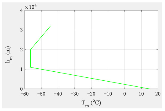
Figure 1.
Relationship between atmospheric temperature and altitude.
(2) Relationship between Atmospheric Pressure and Altitude.
We assumed that the atmosphere was stationary relative to the Earth, i.e., the atmosphere had no movement in the horizontal and vertical directions. According to the knowledge of physics, as the atmosphere was affected by the Earth’s gravity, we used the micro-element method: for a small micro-element atmospheric cylinder with an arbitrary geometric height of h, a cross-sectional area of dS, and a height of dh, the atmospheric pressure difference between its upper and lower surfaces was dP, and the following equation could be determined from the force balance condition:
After sorting, we can obtain:
where g is gravitational acceleration at geometric height h.
In the case that the standard atmosphere was a dry and clean ideal gas, we had:
where P is the pressure when the atmosphere is still; is the air density, and its value is 1.29 kg/m3 under standard conditions (0 °C, 1 standard atmospheric pressure); is the air gas constant, whose value is 287.05287 ; and T is the air temperature.
The relationship between altitude and geometric elements is as follows [20]:
Under standard atmospheric pressure, when considering only the gravitational force, the relationship between available g and gravitational acceleration is as follows:
where = 9.80665, , and = 6,356,766 m, which is the Earth’s polar radius.
According to Equations (1) and (6)–(9) and the reference [21], we can obtain:
where is the corrected atmospheric vertical gradient of the layer (); is the atmospheric pressure of the measurement point (Pa); is the atmospheric pressure of the reference datum (Pa); and is the height value of the reference datum plane (m). Usually, we choose the mean sea level as the corresponding reference point; then, under standard atmospheric pressure, =101.352 KPa, and mean sea level height = 0. Figure 2 shows the relationship between pressure and altitude when most aircraft are within 20,000 m.
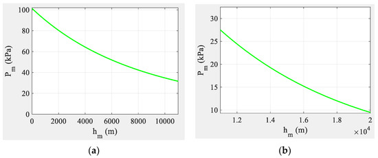
Figure 2.
Relationship between atmospheric pressure and altitude within 20,000 m: (a) 0~11,000 m, (b) 11,000~20,000 m.
2.1.2. Altimeter-Assisted Positioning Algorithm
(1) Analysis of the Influence of Temperature and Atmospheric Pressure on Elevation Measurement.
According to the analysis in Section 2.1.1, we knew that temperature and atmospheric pressure would have different effects on the distribution of different altitudes; thus, they will also have a certain impact on the actual elevation measurement. According to the results of Figure 1 and Figure 2, for a high-speed flying aircraft, the faster the flight speed and the higher the climb height, for long-term flight operations (such as one month or even one year), it was evident that the changes in atmospheric pressure and temperature would fluctuate more due to changes in climatic conditions. If the change was large, it would bring great errors to the elevation measurement. However, this kind of flying operation is usually very rare in practice. For most flight operations, the time is not very long due to the power factor, and the flight operations can usually be completed within a few hours or even tens of minutes. Therefore, we started from a short-term perspective to study the effect of temperature and atmospheric pressure on elevation measurement. Figure 3, Figure 4 and Figure 5 present open data from the China central meteorological observatory [22], showing temperature and atmospheric pressure in the northern hemisphere at 1 h intervals, starting at noon Beijing time on 27 March 2022. For real-time forecast results, we extracted the display results with intervals of 20 min, 30 min, and 1 h.
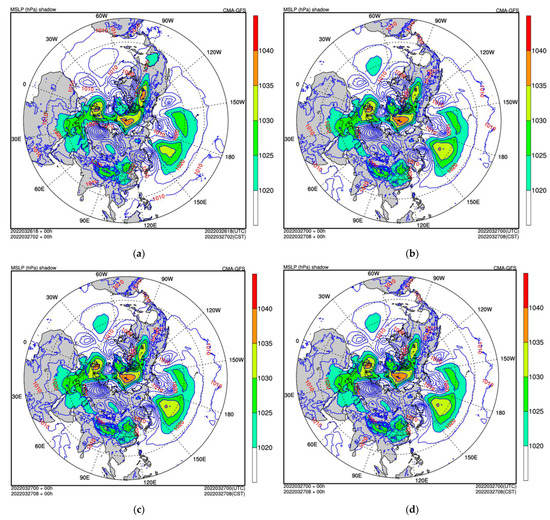
Figure 3.
Real-time atmospheric pressure at sea level on 27 March 2022 (Beijing time): (a) 12:30, (b) 12:50, (c) 13:00, (d) 13:30.
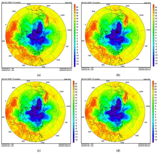
Figure 4.
Real-time temperature at 850 hPa altitude on 27 March 2022 (Beijing time): (a) 12:30, (b) 12:50, (c) 13:00, (d) 13:30.
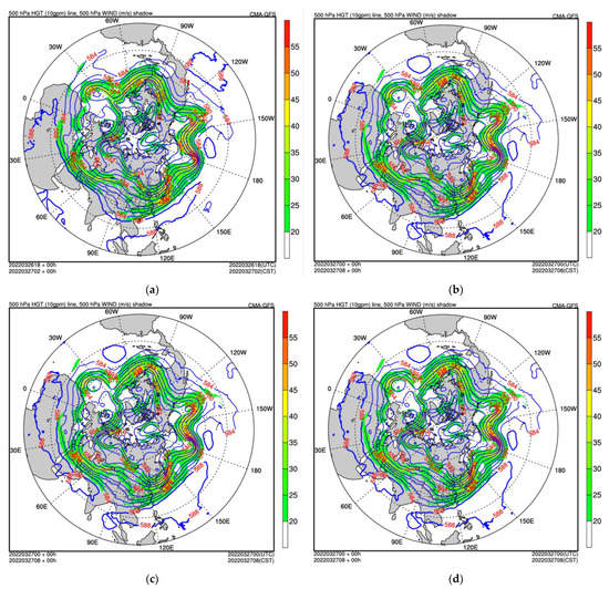
Figure 5.
Real-time atmospheric pressure at 500 hPa altitude on 27 March 2022 (Beijing time): (a) 12:30, (b) 12:50, (c) 13:00, (d) 13:30.
Looking at Figure 3, Figure 4 and Figure 5, it is not difficult to find that the temperature and atmospheric pressure changes are relatively gentle for a point on the northern hemisphere and its zenith elevation (from sea level to 850 hPa (1500 m) to 500 hPa (5500 m)); specifically, we took the fixed positions of 0 deg longitude and 60 deg latitude and their zenith elevations. According to Figure 3, the real-time mean sea level pressure (MSLP) at 12:30~13:30 is about 103.25 KPa, and it can be seen that the pressure change is quite gentle. Thus, the atmospheric pressure change obtained by the measurement time interval is about 0, and the influence on the elevation measurement is very small. In addition, the corresponding temperature on the day of the query is 8 °C [22]. According to Figure 4, the real-time mean temperature (TEMP) at the height of 850 hPa is about 2 °C. It can also be seen that the temperature change is also very stable, and the temperature difference obtained by the measurement time interval is also about 0; thus, the elevation measurement error caused by the temperature is also very small. Therefore, in practice, we can use the temperature of the observation point to replace the temperature of the reference point. According to Figure 5, the real-time MSLP at a height of 500 hPa is about 56.4 KPa, and the atmospheric pressure change is very gentle at this time; similarly, the atmospheric pressure difference caused by elevation measurement error is also very small. From sea level to 850 hPa, the altitude increases by 1500 m, and the corresponding temperature decreases by about 6 °C, which is essentially consistent with the theoretical value of Equation (2). Based on this, we give a calibration method for barometric elevation measurement that is convenient for practical use.
(2) Initialization and Calibration of Barometric Altimeter.
The key to elevation measurement is the initial calibration of the barometric altimeter. Here, we omit the solution and derivation process of the dilution of precision (DOP), and the geographic coordinate system adopts the local navigation coordinate system, i.e., the east-north-up (ENU) coordinate system, and we directly give the covariance matrix of the expected error value in each direction of the ENU coordinate system as follows [23]:
where represents the variance of the corresponding aircraft ranging error. Focusing on the diagonal of the matrix, according to the position dilution of precision (PDOP) [24], we can obtain:
In addition, from the above analysis of the influence of temperature and atmospheric pressure on elevation measurement, it can be seen that pressure and temperature change slowly in a short period of time; accordingly, we present a practical correction method as follows.
When the availability of the satellite navigation system is high, i.e., taking the PDOP ≤ 6 in Equation (12) as the service availability threshold then the barometric altimeter is initialized and corrected. The GNSS receiver altitude solution value is used as the initial reference altitude of the barometric altimeter; the temperature and barometric pressure measured by the barometric altimeter are used as the reference temperature and barometric pressure; and, in the subsequent measurement, , , and are used as reference correction values.
After the barometric altimeter is calibrated, by measuring the ambient atmospheric pressure of the aircraft in real time, the real-time altitude of the aircraft is calculated according to Equation (10). After the real-time altitude is obtained, combined with Equation (1), the atmospheric temperature of the environment where the aircraft is located can be obtained. In addition, it should be noted that since the number of satellites is larger in the LEO constellation than the MEO constellation, in the case of SpaceX, it is at least 100 times that of the GPS constellation. Therefore, when the LEO constellation is used for navigation and positioning, PDOP ≤ 6 is a conventional usability constraint. With the advantage of the large number of LEO satellites, the threshold value can be relaxed according to the required accuracy level so that the shielding angle can be increased to suppress the adverse effects of multipath interference. Using this method does not require the meteorological reference station to correct the altitude of the aircraft. As altitude is measured relative to reference point , the distance between the measurement position and the reference point is relatively close, which avoids the elevation error caused by the inconsistency between the geoid and the ellipsoid.
(3) Improving Geometric Precision Factor by Eliminating Clock Bias.
Consistent with the algorithm [12,25,26], we assume that the clock bias between the aircraft and the broadband LEO satellite has been eliminated; therefore, according to the principle of navigation and positioning, only three visible satellites are needed to solve for the user’s location. More importantly, according to Equation (11) and the definition of the vertical dilution of precision (VDOP) [27], we can obtain:
At this point, we find that when the clock bias is eliminated, VDOP is a matrix independent of clock bias (the same is true for other accuracy factors), and, as we can see, it can be seen that the value of VDOP will be significantly improved. Although the vertical positioning accuracy of the satellite navigation system is poor, it can be improved to a certain extent with the assistance of clock bias elimination, which can provide an accurate reference for correction of the barometric altimeter.
(4) Aircraft Location Solution.
After completing the correction and acquisition of the aircraft’s elevation information, the next step is to solve the real-time position of the aircraft. We use the WGS84 coordinate system to model the Earth, and we regard the Earth as a flat spheroid. If the aircraft’s ECEF coordinates are , it satisfies the following ellipsoid equation [28]:
where , , and are the Earth’s equatorial radius, with a value of 6378.1370 km, and is the polar radius of the Earth.
According to Equations (10) and (14), and combining the pseudo-range measurement information, we can complete the aircraft’s position calculation.
2.1.3. Acquiring of LEO Satellite Ephemeris and Calculating LEO Satellite Position
The satellite ephemeris is the information describing the orbit of the satellite; it can also be described as a set of orbital parameters corresponding to a certain moment. With the satellite ephemeris, we can calculate the position and velocity of the satellite at any time. When we know the position and velocity of the satellite, we can establish the relevant pseudo-range observation equation to solve the unknown position of the user.
(1) Acquiring LEO Satellite Ephemeris.
A GNSS satellite ephemeris is divided into forecast ephemeris and postprocessing ephemeris. The forecast ephemeris is also called the broadcast ephemeris, which is real-time ephemeris data. Generally, through the broadcast ephemeris, we can calculate the current or future satellite position within 2 h; postprocessing can obtain higher precision ephemeris from the International GNSS Service (IGS), which can provide the precision ephemeris (IGS final), fast precision ephemeris (IGS rapid), and ultrafast precision ephemeris (IGS ultrarapid) [29].
The accuracy of the IGS final ephemeris is the highest, and the update rate is one week, but the data delay is longer, requiring 13 days.
The data accuracy of the IGR ephemeris is basically the same as that of IGS final, with an update rate of one day and a data delay of 17 h.
The IGU ephemeris data are divided into two parts: real-time and predicted satellite ephemeris, each 24 h in length. The real-time ephemeris needs to be delayed by 3 h, while the predicted satellite ephemeris is based on the satellite ephemeris of the previous 24 h to predict the satellite ephemeris of the next 24 h.
Considering that the orbital period of LEO satellites is relatively short, being, generally, approximately 2 h, and the time to cross the zenith is generally only 10 min, to ensure real-time navigation and positioning calculations, it is evident that the IGS final, IGR, and IGU ephemeris are not suitable. Although the IGU ephemeris has a real-time satellite ephemeris part, it is also suitable for real-time processing applications, but the trade-off is a large error, thus it is not suitable for LEO satellites. Therefore, to ensure the real-time performance of navigation and positioning, we chose a broadcast ephemeris similar to GPS as the LEO broadcast ephemeris.
(2) Solving LEO Satellite Position and Velocity.
Through the six orbital elements and nine perturbation parameters of the LEO satellite (see Table 2 for specific parameters), here, the LEO constellation uses the Walker constellation configuration. We can calculate the position and velocity information of the satellite. After obtaining the position information, the velocity can be obtained by determining the difference in satellite positions at adjacent times. It is also possible to obtain the velocity directly by taking the derivative of the position of the satellite.
Table 2.
Relevant ephemeris parameters in LEO satellite navigation messages.
2.2. INS+ Three LEO Satellite (LEO3) Dynamic Switching Integrated Navigation and Positioning Algorithm with Clock Bias Cancellation and Altimeter Assistance
2.2.1. Overall Algorithm Block Diagram
The three LEO satellite dynamic switching range INS integrated navigation and positioning algorithm with clock bias cancellation and altimeter assistance can be divided into two types: the first, with three satellites participating in the dynamic switching and alternately using real and virtual range values, and the second, also with three satellites, where one uses continuous real range values and the other two dynamically switch between real and virtual range values. The definitions of real and virtual range values will be defined in subsequent sections. Before introducing the algorithms, we provide a general block diagram of the two major algorithms, shown in Figure 6.
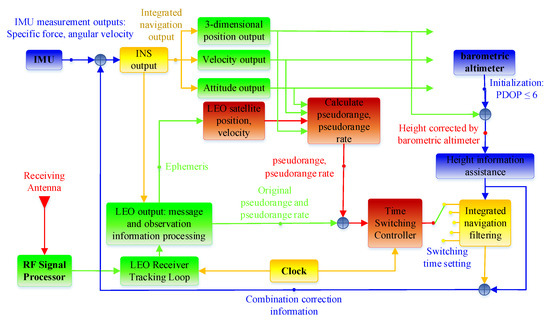
Figure 6.
Overall block diagram of three LEO satellites dynamic switching range integrated navigation and positioning algorithm with clock bias cancellation and altimeter assistance.
In Figure 6, the clock source is the internal clock of the LEO receiver. In addition to providing a precise clock source for the receiver, it is also used for dynamic switching of the precise clock source of the time switching controller.
2.2.2. INS+ LEO3 Dynamic Switching Range + Altimeter-Integrated Navigation Algorithm
Based on the GDOP satellite selection principle [30], we chose three broadband LEO satellites in the same orbit that are always visible during the aircraft’s flight movement, named LEO#1, LEO#2, and LEO#3. Let the virtual pseudo-range measurement values between the broadband LEO satellite and the INS obtained by the INS solution be , , and at this time, and the corresponding aircraft ECEF position coordinates obtained by the INS are . Let , , and denote the virtual pseudo-range measurement values between the broadband LEO satellite and the aircraft obtained by the INS through a real-time extrapolation measurement; at this time, the aircraft’s ECEF coordinate position obtained by the INS real-time extrapolation measurement is . Let , , and denote the real pseudo-range measurement values between the broadband LEO satellite and the aircraft calculated by the broadband LEO satellite ephemeris, respectively, and the aircraft’s ECEF real coordinate position obtained through the pseudo-range information is . The user’s elevation can be obtained by real-time measurement through the barometric altimeter carried by the user.
Next, considering that the time for broadband LEO satellites to pass the zenith is generally about 10 min [2], we must dynamically switch between satellites to ensure more reliable location services. In addition, to save the beam bandwidth of broadband LEO satellites, avoid long-term occupation of bandwidth resources, and prevent them from ceasing to work due to satellite failure in extreme cases, we must also dynamically switch the satellite. The specific method is to dynamically switch the virtual measurement values , , and real pseudo-range measurement values , , , where the virtual range value is defined as the range value obtained by INS, and the real range value is defined as the range value obtained by satellite ephemeris [31]. Subsequently, supplemented by the corresponding elevation measurement value for integrated navigation and positioning, we assume that the dynamic switching interval is , and can be set according to actual needs. See Figure 7 for detailed schematic diagram of dynamic switching. Next, we describe the flow of the algorithm in detail.
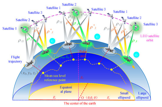
Figure 7.
Schematic diagram of INS+ LEO3 dynamic switching range integrated navigation algorithm with altimeter.
At time , broadband LEO#1 satellite adopts the real pseudo-range measurement value , and LEO#2 and LEO#3 satellites adopt the virtual pseudo-range measurement values and , thus, at this time:
The pseudo-range measurement information obtained by the INS solution is:
Combining Equations (10) and (14) we can obtain the elevation-assisted measurement information:
where , and is the height value obtained by INS measurement; ; ; is the height measured by the altimeter; and .
We subtract the corresponding terms of Equations (15) and (16), determine the difference between the two terms in Equation (8), and then divide them:
Subsequently, based on the unscented Kalman filter (UKF) algorithm, we adopt the differences , , , and in Equation (18) as the observation information of the tight integrated navigation system for filtering, in order to obtain the optimal estimates of the broadband LEO satellite and INS systems and, finally, obtain the aircraft’s position.
Similarly, at moments and , according to the dynamic switching time interval, the real pseudo-range measurement values of broadband LEO#2 and LEO#3 are used in turn, while the remaining satellites use virtual pseudo-range measurement values supplemented by elevation information, and then this process is cycled until the end of the user runtime.
The next processing flow is the process in dynamic loop ~ until the end of the simulation time of the entire system.
2.2.3. INS + Two LEO Satellites Dynamic Switching Range Integrated Navigation Algorithm with LEO3 (LEO3-2) + Altimeter
The basic idea of the algorithm is similar to what is described in Section 2.2, but the difference is that one satellite keeps the true pseudo-range measurement value (such as LEO#1 satellite, but it will also change with dynamic switching), while the other two satellites perform dynamic switching ranging based on the real and e virtual pseudo-range measurement values under the three dynamically switched broadband LEO satellites. Similarly, we only consider dynamic switching under the same orbit. See Figure 8 for the specific dynamic switching algorithm. Next, we will describe the specific process of the algorithm; without loss of generality, we let the broadband LEO#1 satellite use continuous real pseudo-range measurements.
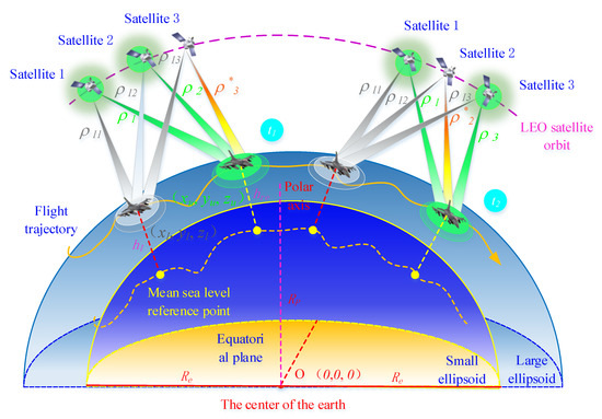
Figure 8.
Schematic diagram of INS + two LEO satellites dynamic switching range integrated navigation algorithm with LEO3 (LEO3-2) + altimeter.
At time , the LEO #1 and LEO #2 satellites adopt the real pseudo-range measurement values and , and LEO #3 adopts the virtual pseudo-range measurement value . At this time:
We subtract the corresponding terms of Equations (19) and (16), combine and determine the difference between the two terms in Equation (17), and then divide them. Thus, we can obtain:
Similarly, the subsequent processing flow is consistent with the description of time in Section 2.2.
Similarly, at time , the real pseudo-range measurements values are used for LEO#1 and #3, and the virtual pseudo-range measurements value are used for LEO#2. The next processing flow is the processing in dynamic loop ~ until the end of the simulation time of the entire system.
2.3. Disturbance and Combination Model
2.3.1. LEO Orbit Perturbation Model
According to Figure 9 and Reference [12], relative to other orbital constellations, such as inclined geosynchronous orbit (IGSO) satellites, geosynchronous orbit (GSO) satellites, and MEO satellites, the perturbations suffered by LEO satellites mainly include non-spherical perturbations of the Earth and drag perturbations of the Earth’s atmosphere.
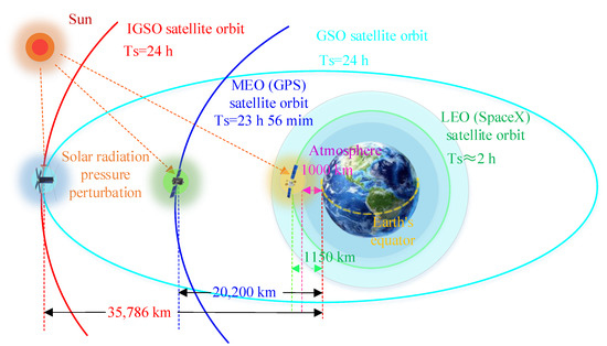
Figure 9.
Schematic diagram of main perturbations in LEO constellation orbit.
For non-spherical perturbations of the Earth, the specific model is [12,32]:
where is the satellite position offset caused by 24 h of the non-spherical perturbation of the Earth; represents the initial phase of the perturbation; is the operating cycle of the LEO constellation; k is the linear deviation constant of the orbit; M is the number of operating cycles of the LEO satellite; is a fixed constant; is the perturbation accuracy, here = 1; and is random noise, with a mean of 0 and a variance of 1. In addition, the model uses the joint gravity model family 3 (JGM3) of models in the fitting with an order of 70 × 70 [33].
For drag perturbations of the Earth’s atmosphere, the change in position offset caused by atmospheric drag perturbation is also slightly periodic but not significant. Therefore, we do not use a periodic function to model it here. In addition, the increase in position offset caused by atmospheric drag perturbation is nonlinear, and the growth rate will gradually accelerate over time, which strengthens its influence. The specific model is [32]:
According to Equations (21) and (22), the total perturbation suffered by the LEO satellite is .
2.3.2. Combination and Environmental Disturbance Models
Regarding the integrated navigation model of the system, we use the strapdown inertial navigation system model for the inertial navigation model. The detailed model is consistent with the algorithm [12]; the state and measurement equations of the entire system can be found in [12,31], and, due to space limitations, we will not describe it in much detail here. In addition, the environmental model and multipath interference models refer to [34,35,36,37,38,39,40], and we will not list the specific models here.
3. Experimental Results and Analysis
3.1. Experimental Parameter Settings
This algorithm adopted the main constellation of 1600 broadband LEO satellites in the SpaceX constellation for experiments. See Table 3 for related parameters [32,41,42] and Table 4, Table 5 and Table 6 for other simulation parameters [43,44]. Among them, we took the aircraft as an example for simulation, but this did not affect the generality of the simulation experiment; it was applicable to other users such as land vehicles, ships, and pedestrians.
Table 3.
SpaceX main constellation parameter settings.
Table 4.
Main initial parameter settings of UKF and aircraft trajectory.
Table 5.
Setting of main parameters of IMU.
Table 6.
Selection of broadband LEO satellites and setting of altimeter deviation parameters.
3.2. INS + LEO3 Dynamic Switching Range Integrated Navigation Algorithm + Unbiased Altimeter
According to the algorithm principle described in Section 2.2.2 and the relevant parameter settings in Section 3.1, we abbreviated the INS algorithm with three broadband LEO satellites in the same orbit with dynamic switching range and altimeter-integrated navigation with altimeter as: Un-Alt s, where s represented the dynamic switching time, and the values are shown in Table 6. The experimental results are shown in Figure 10. To improve the problem of large navigation and positioning errors caused by the algorithm [12] when the broadband LEO satellites were in the same orbit, as a comparison, we also took the algorithm proposed in [12] for simulation comparison, and abbreviated it as No-Alt s switching, where the meaning of was the same as in Un-Alt s. Since the multipath model was difficult to express with analytical formulas, we set the satellite elevation angle to 10° (see Table 6) to simulate the broadband LEO satellite signal being affected by multipath effects and continued to use this rule in subsequent simulations. Specifically, EPE in the figure represents east position error and EVE represents east velocity error; the meanings of other abbreviations can be deduced by analogy.
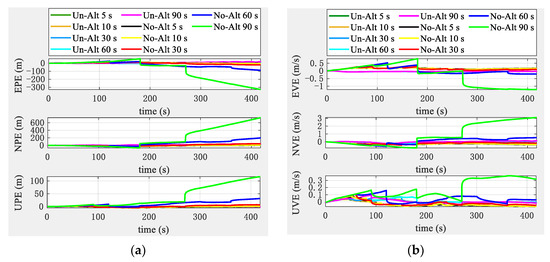
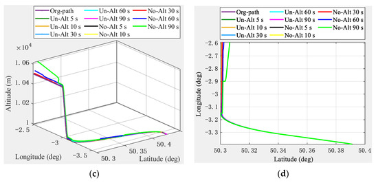
Figure 10.
Error curves of INS + LEO3 dynamic switching range + unbiased altimeter-integrated navigation algorithm + unbiased altimeter under the same orbit: (a) position error; (b) velocity error; (c) three-dimensional trajectory error; (d) two-dimensional trajectory error.
From Figure 10, we can see that adopting a high-precision altimeter can effectively improve the corresponding position and velocity errors, especially in the case of long dynamic switching time, and the effect of improving the up error is very evident. At the same time, the divergence suppression effect of the pure INS navigation error is also better. Judging from the final three-dimensional and the two-dimensional trajectory error curves, the algorithm after adding the altimeter may be closer to the aircraft’s real flight trajectory. To quantitatively analyze the difference between the two algorithms, we calculated statistics on the mean and standard deviation (STD) of the final three-dimensional trajectory curve error and conducted a comparative analysis; the statistical results are shown in Table 7.
Table 7.
Error index comparison of INS + LEO3 dynamic switching range integrated navigation algorithm + unbiased altimeter.
From Table 7, we can see that the INS + LEO3 alternate switching algorithm that does not rely on an altimeter has large indicators of incoherent mean or STD of longitude, latitude, and altitude errors, especially when the switching time is 90 s, the mean value and STD of the altitude are about 37 m and 41 m, respectively, when the dynamic switching time is long. When we add an altimeter, these error indices are reduced to 0.0268 m and 0.5784 m, respectively. It can be seen that the addition of an altimeter results in a very significant improvement in the vertical direction, mainly due to the elimination of clock bias between the aircraft and the broadband LEO satellite, which improves the accuracy of the system’s elevation measurement. When an altimeter and clock bias elimination are together used for assistance, the accuracy of the vertical direction depends mainly on the measurement accuracy of the altimeter; here, we chose the altimeter without deviation, and thus the improvement effect is very evident.
3.3. INS+ Two LEO Satellites Dynamic Switching Range Integrated Navigation Algorithm under LEO3 (LEO3-2) + Unbiased Altimeter
Based on the principle of the INS with two LEO satellites, the dynamic switching range integrated navigation algorithm under LEO3 with altimeter described in Section 2.2.3, and the relevant parameters in Section 3.1, we conducted simulation experiments using this algorithm. We also simulated and compared the algorithms proposed in [12]. We divided the algorithm into two scenarios: original (keep one satellite with continuous and real ranging) and comparison (remove continuous and real range satellites). The main purpose of setting up the comparison experiment was to explore the effect of taking continuous and real pseudo-range measurements on navigation and positioning performance. The original experimental simulation results are shown in Figure 11. The corresponding continuous real range satellite was set as LEO #1 satellite (PRN = 209).
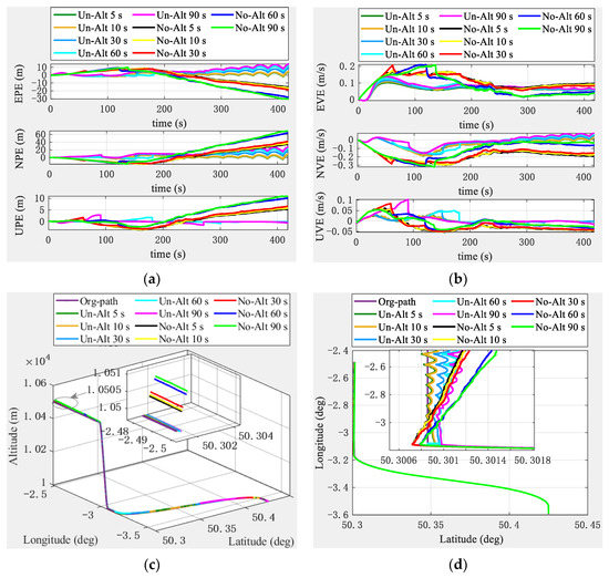
Figure 11.
Error curves of INS+ two LEO satellites dynamic switching range integrated navigation algorithm under LEO3 (LEO3-2) + unbiased altimeter: (a) position error; (b) velocity error; (c) three-dimensional trajectory error; (d) two-dimensional trajectory error.
From Figure 11, we find that both the algorithm in [12] and the algorithm after adding the altimeter can well suppress the divergence of the INS due to the use of a continuous real pseudo-range measurement value; moreover, the difference between the two algorithms in terms of position and velocity error is not very large, due to the fact that both algorithms adopt continuous real pseudo-range measurements to ensure the continuity and stability of navigation and positioning. However, after careful comparison, it can be found that the algorithm with the altimeter has a more concentrated error curve than the algorithm without the altimeter [12]. This also shows that the algorithm is more stable and robust after adding an altimeter, which can be seen from the final three-dimensional and two-dimensional trajectory curves.
As a comparative experiment, we removed the LEO satellite (PRN = 209) with continuous real ranging, and the simulation results are shown in Figure 12.
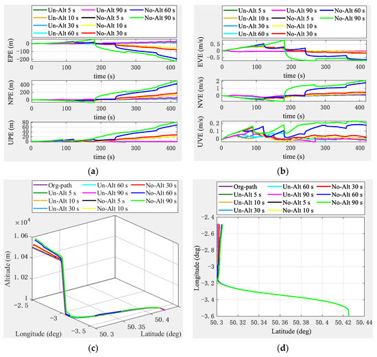
Figure 12.
Comparison of experimental error curves of INS + two LEO satellite dynamic switching range integrated navigation algorithm under LEO3 + unbiased altimeter: (a) position error; (b) velocity error; (c) three-dimensional trajectory error; (d) two-dimensional trajectory error.
From Figure 12, it can be found that the continuity and stability of navigation and positioning cannot be guaranteed due to the removal of the satellite that continues the real ranging in the comparison experiment, which leads to significantly large errors in the navigation and positioning algorithm without the altimeter; however, when the altimeter was added, these larger errors were significantly improved. To compare the error improvement of the original experimental scene (OES or O) and the experimental scenarios (as CES or C), we count the corresponding error indicators shown in Figure 13. For ease of presentation, INS + LEO3-2 + unbiased altimeter + 60 s switching in CES is abbreviated as Un-Alt 60 s|C, and INS + LEO3-2 + 60 s switching in CES is abbreviated as No-Alt 60 s|C; other abbreviations follow the same principle.
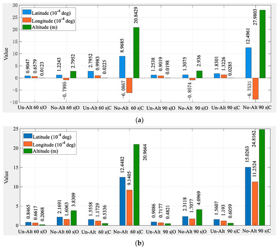
Figure 13.
Comparison of statistical results of error indicators between OES and CES: (a) mean; (b) STD.
From the statistical results in Figure 13, it can be seen that the use of a continuous real range satellite is very important to improve the algorithm’s error; the relevant indicators of CES are significantly worse than OES even if an altimeter is not added. With an altimeter, the error and positioning accuracy are improved. This shows that it will improve the positioning accuracy and positioning stability of the whole system if the pseudo-range measurement value of a continuous LEO satellite can be guaranteed. Therefore, in practical applications, we should try our best to ensure a continuous real pseudo-range measurement, which is not difficult to do for large-scale deployment of LEO constellations.
4. Comparison of Navigation and Positioning Results under Different Altimeter Scenarios
From the analysis in Section 3.2, we know that the vertical accuracy mainly depends on the height measurement accuracy of the altimeter when the clock bias between the aircraft and the broadband LEO satellite is eliminated. However, in actual engineering applications, due to the different requirements for altimeter accuracy, some civilian activities such as adventuring, mountaineering, and other outdoor sports may not need too high altimeter accuracy, while fields such as surveying and mapping, airport precision approach and landing, and others have high requirements for altimeter accuracy. Altimeter deviations can cause unimaginable disasters, such as the crashes of Flight 763 (in 1996, which killed 349 people), Flight BA038 (in 2008, fortunately no deaths), and flight TK1951 (in 2009, causing 9 deaths and 120 injuries) [45,46,47]. Therefore, it is essential for us to explore the impact of altimeter deviations on the accuracy of the algorithm. Based on the actual situation, we divided the altimeter error into a fixed deviation of ±5 m (the accuracy that most manufacturers can easily achieve at present; the precision developed by [48] is about 1 m) and a fixed deviation of ±10 m. Combined with the two cases of unbiased altimeters described in Section 3.2 and Section 3.3, we explored the navigation and positioning performance of different algorithms in different altimeter deviation scenarios in order to provide a reference basis for practical engineering applications. We fixed the dynamic switching time to 60 s for experimentation, and the results are shown in Figure 14.
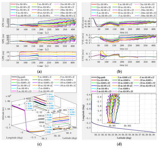
Figure 14.
Algorithm error comparison curves under different altimeter deviation scenarios: (a) position error; (b) velocity error; (c) three-dimensional trajectory error; (d) two-dimensional trajectory error.
From Figure 14, we can see that the corresponding error will also increase as the altimeter deviation increases, but they are all within the acceptable range, and the final error shows a trend in convergence. In general, the effect is best when the altimeter has no deviation, which is expected, and the fixed deviation ±5 m is second, ±10 m again, but the navigation and positioning algorithm errors in the ±5 m and ±10 m altimeter situations are both within an acceptable range, which can meet the needs of actual location services. Furthermore, with the same altimeter deviation, the OES performance is the best among the three algorithms, while the CES is the worst. Therefore, in practical engineering applications, in addition to choosing between cost and accuracy combined with the specific needs of the situation, we should also ensure the continuous real range value of LEO as much as possible.
5. Comparison with Other Algorithms
To verify the effect of our algorithm, we combined the INS + three-satellite dynamic switching range integrated navigation and positioning algorithm with the LEO constellation with the elimination of clock bias and altimeter assistance, the three-satellite alternate switching algorithms without altimeter assistance, the traditional three-satellite integrated navigation algorithms with altimeters (Traditional MEO3 + Alt), and the typical advanced four-satellite algorithm (MEO4 fusion) for comparison to verify the advantages and disadvantages of our algorithm. Our algorithm considers the dynamic switching of three LEO satellites (LEO 3) in the same orbit, and one of the three satellites adopts continuous real pseudo-range measurements while the other adopt the real and virtual pseudo-range measurement values for dynamic switching (LEO3-2). The switching time was set to the longer 60 and 90 s, the unbiased altimeter was used for assistance, and the corresponding algorithms were abbreviated as: Un-Alt 60 s, Un-Alt 90 s, Un-Alt 60 s|O, and Un-Alt 90 s|O, respectively. Similarly, the algorithms with alternative switching of LEO 3 and LEO 3-2 without altimeters assistance were abbreviated as: No-Alt 60 s, No-Alt 90 s, No-Alt 60 s|O, and No-Alt 90 s|O, respectively [12]. The traditional algorithm using three MEO satellites and an altimeter and the typical algorithm with the fusion of four or more MEO satellites are abbreviated as: Traditional MEO3+ Alt [49] and MEO4 fusion [50], respectively. We calculated statistics on the comparison indicators, with the conversion of some units uniformly processed according to [51], and the results are shown in Figure 15.
where is the average radius of the Earth, and its value is 6,371,393 m.
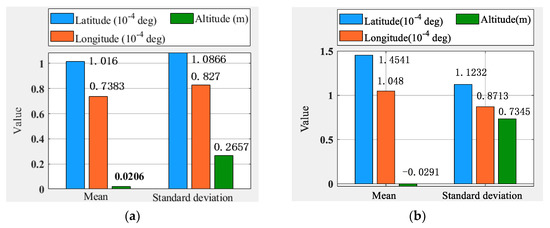
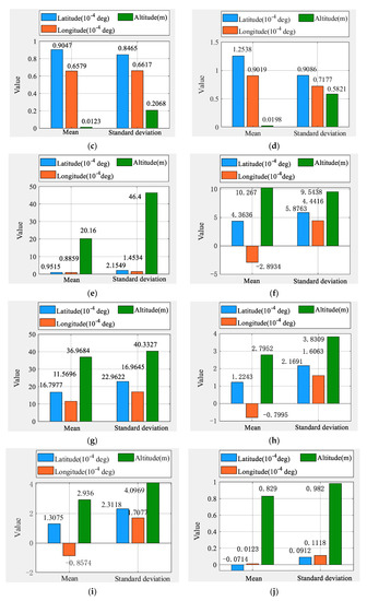
Figure 15.
Comparison of statistical results with other algorithms: (a) Un-Alt 60 s, (b) Un-Alt 90 s, (c) Un-Alt 60 s|O, (d) Un-Alt 90 s|O, (e) Traditional MEO3+Alt, (f) No-Alt 60 s, (g) No-Alt 90 s, (h) No-Alt 60 s|O, (i), No-Alt 90 s|O (j) MEO4 fusion.
The following can be seen from the statistical comparison results in Figure 15:
- (1)
- Our algorithm was significantly better than the traditional MEO3+ altimeter-integrated navigation algorithm for various statistical indicators. This also confirmed that the navigation and positioning accuracy based on the LEO constellation was better than that of the MEO constellation under the same number of observation satellites.
- (2)
- Our algorithm could, to a large extent, overcome the large positioning error caused by the alternate switching of three LEO satellites without altimeter assistance (including LEO3 and LEO3-2) when the switching time was long, and the 90 s switching time under LEO3 was the most evident. The mean and standard deviation of longitude were increased by 91.34 and 95.11%, the mean and standard deviation of latitude were increased by 90.94 and 94.86%, and the altitude indices were increased by 99.92 and 98.18%.
- (3)
- Although our algorithm was slightly inadequate in longitude and latitude indicators compared with some typical advanced fusion algorithms for 4 MEO satellites, this result was expected since these algorithms had sufficient visible satellites. When some advanced sensors were used for fusion, the accuracy would, naturally, be greatly improved. Our foothold was a low-cost navigation solution with a conservative selection of sensor model parameters. In addition, our switching time selection was relatively large; thus, the result was evident. However, our algorithm could be significantly better than the MEO4 star fusion algorithm in terms of high performance, and this was mainly due to the altimeter calibration method that we used.
- (4)
- Compared with the algorithm that did not adopt continuous real pseudo-range measurement values, the algorithm that did adopt these values had an advantage in each accuracy index. This was not difficult to understand because the use of continuous real pseudo-range measurement values could ensure the reliability and robustness of the entire system.
Therefore, through the comparison of the above algorithms, it was verified that our algorithm potentially had great advantages in accuracy, which meant it could be used as a reference solution to provide aircraft with continuous navigation and positioning services in challenging environments such as cities, valleys, and forests.
6. Conclusions
Based on the analysis of temperature, atmospheric pressure, and altitude, we concluded that temperature and atmospheric pressure have little effect on the elevation measurement in a short period of time. On this basis, we proposed an altimeter initialization correction method without the auxiliary correction of the weather station. Then, based on clock bias elimination, the LEO satellite dynamic switching scheme aided by an altimeter could improve the problem of an excessive cumulative error caused by too long of a switching time, and the accuracy of navigation and positioning could be greatly improved. At the same time, it could ensure the continuity and stability of navigation and positioning. In addition, as the accumulated error caused by the long switching time was reduced, we could continue to increase the time interval of dynamic switching, taking into account the navigation function of the ICN technology without affecting its communication function, which could ensure a sufficient navigation and communication service time.
Although altimeters with different precision values would lead to an increase in positioning error with an increase in fixed deviation, the errors were all within the acceptable range, which could meet actual location service needs. Compared with traditional algorithms and advanced four-satellite fusion algorithms, our proposed algorithm also had certain advantages related to various accuracy indicators. Therefore, our proposed algorithm could be used as a three-satellite location service reference scheme in the case of incomplete visible satellites. However, the LEO satellites move too fast, which is a challenging research topic in terms of the acquisition of large dynamic GNSS signals, the selection of signal frequency bands, and adaptive switching between different LEO satellites.
Author Contributions
Conceptualization, L.Y. and Y.Y.; Methodology, L.Y. and Y.Y.; Software, L.Y.; Validation, L.Y. and Y.Y.; Formal Analysis, L.Y., N.G., Y.Y., L.D. and H.L.; Investigation, L.Y., N.G. and L.D.; Re-sources, Y.Y. and H.L.; Data Curation, L.Y., N.G. and L.D.; Writing—Original Draft Preparation, L.Y.; Writing—Review and Editing, L.Y., N.G., L.D., Y.Y. and H.L.; Visualization, L.Y.; Supervision, Y.Y. and H.L.; Project Administration, Y.Y.; All authors discussed the results, reviewed the manuscript and approved the final manuscript. All authors have read and agreed to the published version of the manuscript.
Funding
Funding was provided by the National Key Research and Development Program of China (grant no. 2017YFC1500904, 2016YFB0501301), the National 973 Program of China (grant nos. 613237201506), the Advance Research Project of Common Technology (no. 41418050201), and the Open Research Fund of Southwest China Institute of Electronic Technology (no. H18019).
Data Availability Statement
Not applicable.
Conflicts of Interest
The authors declare no conflict of interest.
References
- Li, M.; Xu, T.; Ge, H.; Guan, M.; Yang, H.; Fang, Z.; Gao, F. LEO-Constellation-Augmented BDS Precise Orbit Determination Considering Spaceborne Observational Errors. Remote Sens. 2021, 13, 3189. [Google Scholar] [CrossRef]
- Smith, P. Commercial Space Transportation: Recent Trends and Projections for 2000–2010. In The Space Transportation Market: Evolution or Revolution? Space Studies; Rycroft, M., Ed.; Springer: Dordrecht, The Netherlands, 2000; p. 5. [Google Scholar] [CrossRef]
- Caceres, M. LEO mobiles: The next generation. Aerosp. Am. 2007, 45, 18–20. [Google Scholar]
- Reid, T.; Neish, A.M.; Walter, T.; Enge, P.K. Broadband LEO Constellations for Navigation. Navigation 2018, 65, 205–220. [Google Scholar] [CrossRef]
- Leyva-Mayorga, I.; Soret, B.; Röper, M.; Wübben, D.; Matthiesen, B.; Dekorsy, A.; Popovski, P. LEO Small-Satellite Constellations for 5G and Beyond-5G Communications. IEEE Access 2020, 8, 184955–184964. [Google Scholar] [CrossRef]
- Li, J.; Lu, H.; Xue, K.; Zhang, Y. Temporal Netgrid Model-Based Dynamic Routing in Large-Scale Small Satellite Networks. IEEE Trans. Veh. Technol. 2019, 68, 6009–6021. [Google Scholar] [CrossRef]
- Tai, J.; Lv, J.; Wu, X.; Song, T.; Zhang, Q.; Xiang, Y.; Sun, J. Topology optimization Design of LEO Satellite Network. In Proceedings of the 2019 Chinese Control Conference (CCC), Guangzhou, China, 27–30 July 2019; pp. 8154–8159. [Google Scholar]
- Papa, A.; De Cola, T.; Vizarreta, P.; He, M.; Machuca, C.M.; Kellerer, W. Dynamic SDN Controller Placement in a LEO Constellation Satellite Network. In Proceedings of the 2018 IEEE Global Communications Conference (GLOBECOM), Abu Dhabi, United Arab Emirates, 9–13 December 2018; pp. 206–212. [Google Scholar]
- Reid, T. Orbital Diversity for Global Navigation Satellite Systems. Ph.D. Thesis, Stanford University, Stanford, CA, USA, 2017. [Google Scholar]
- Morales, J.J.; Khalife, J.; Cruz, U.S.; Kassas, Z.M. Orbit Modeling for Simultaneous Tracking and Navigation using LEO Satellite Signals. In Proceedings of the 32nd International Technical Meeting of the Satellite Division of The Institute of Navigation (ION GNSS+ 2019), Miami, FL, USA, 16–20 September 2019; pp. 2090–2099. [Google Scholar]
- Ye, L.; Yang, Y.; Jing, X.; Ma, J.; Deng, L.; Li, H. Single-Satellite Integrated Navigation Algorithm Based on Broadband LEO Constellation Communication Links. Remote Sens. 2021, 13, 703. [Google Scholar] [CrossRef]
- Ye, L.; Gao, N.; Yang, Y.; Li, X. A High-Precision and Low-Cost Broadband LEO 3-Satellite Alternate Switching Ranging/INS Integrated Navigation and Positioning Algorithm. Drones 2022, 6, 241. [Google Scholar] [CrossRef]
- Orabi, M.; Khalife, J.; Kassas, Z.M. Opportunistic Navigation with Doppler Measurements from Iridium Next and Orbcomm LEO Satellites. In Proceedings of the 2021 IEEE Aerospace Conference (50100), Virtual, 6–13 June 2021; pp. 1–9. [Google Scholar] [CrossRef]
- Khalife, J.; Neinavaie, M.; Kassas, Z.M. Blind Doppler Tracking from OFDM Signals Transmitted by Broadband LEO Satellites. In Proceedings of the 2021 IEEE 93rd Vehicular Technology Conference (VTC2021-Spring), Virtual, 25–28 April 2021; pp. 1–5. [Google Scholar] [CrossRef]
- Khalife, J.J.; Kassas, Z.M. Receiver Design for Doppler Positioning with LEO Satellites. In Proceedings of the ICASSP 2019–2019 IEEE International Conference on Acoustics, Speech and Signal Processing (ICASSP), Brighton, UK, 12–17 May 2019; pp. 5506–5510. [Google Scholar]
- Zhao, Y.; Cao, J.; Li, Y. An Improved Timing Synchronization Method for Eliminating Large Doppler Shift in LEO Satellite System. In Proceedings of the 2018 IEEE 18th International Conference on Communication Technology (ICCT), Chongqing, China, 8–11 October 2018; pp. 762–766. [Google Scholar]
- Yang, Z.; Shen, Y.; Shi, X.; Wang, Y. Joint Time Synchronization and Ranging Method Aided by Doppler Frequency Shift. In Proceedings of the 2022 IEEE 10th Joint International Information Technology and Artificial Intelligence Conference (ITAIC), Chongqing, China, 17–19 June 2022; pp. 1616–1621. [Google Scholar]
- Groves, P.D. Principles of GNSS, Inertial, and Multisensor Integrated Navigation Systems, 2nd ed.; Artech House: Fitchburg, MA, USA, 2012; 776p, ISBN 978-1-60807-005-3. [Google Scholar]
- Seddon, J.M.; Newman, S. The Basics of Aerodynamics; National Defense Industry Press: Arlington, Virginia, 2009; 307p, ISBN 978-7-118-06532-9. [Google Scholar]
- Hao, Z. Research Techniques of Instrument Based on Integrated Sensors. Ph.D. Thesis, Nanjing University of Aeronautics and Astronautics, Nanjing, China, 2010. [Google Scholar]
- Osder, S.S. Air-Data Systems, 2nd ed.; John Wiley & Sons: Hoboken, NJ, USA, 1997. [Google Scholar] [CrossRef]
- National Meteorological Center of China. Available online: http://www.nmc.cn (accessed on 1 March 2022).
- Ye, L.; Yang, Y.; Jing, X.; Li, H.; Yang, H.; Xia, Y. Altimeter + INS/Giant LEO Constellation Dual-Satellite Integrated Navigation and Positioning Algorithm Based on Similar Ellipsoid Model and UKF. Remote Sens. 2021, 13, 4099. [Google Scholar] [CrossRef]
- Grewal, M.S.; Andrews, A.P.; Bartone, C.G. Global Navigation Satellite Systems, Inertial Navigation, and Integration, 4th ed.; John Wiley & Sons: Hoboken, NJ, USA, 2020; 608p, ISBN 978-1-119-54783-9. [Google Scholar]
- Ye, L.; Yang, Y.; Ma, J.; Deng, L.; Li, H. A Distributed Formation Joint Network Navigation and Positioning Algorithm. Mathematics 2022, 10, 1627. [Google Scholar] [CrossRef]
- Ye, L.; Yang, Y.; Ma, J.; Deng, L.; Li, H. Research on an LEO Constellation Multi-Aircraft Collaborative Navigation Algorithm Based on a Dual-Way Asynchronous Precision Communication-Time Service Measurement System (DWAPC-TSM). Sensors 2022, 22, 3213. [Google Scholar] [CrossRef]
- Chen, J.; Huang, J.; An, X. Satellite Navigation Positioning and Anti-Jamming Technology; Publishing House of Electronics Industry: Beijing, China, 2016; 245p, ISBN 978-7-121-29150-0. [Google Scholar]
- Groves, P.D. Principles of GNSS, Inertial, and Multisensor Integrated Navigation Systems; Artech House: Fitchburg, MA, USA, 2008; 503p, ISBN 978-1-58053-255-6. [Google Scholar]
- Tusat, E.; Ozyuksel, F. Comparison of GPS satellite coordinates computed from broadcast and IGS final ephemerides. Int. J. Eng. Geosci. 2018, 3, 12–19. [Google Scholar] [CrossRef]
- Zhang, M.; Zhang, J. A Fast Satellite Selection Algorithm: Beyond Four Satellites. IEEE J. Sel. Top. Signal Process. 2009, 3, 740–747. [Google Scholar] [CrossRef]
- Ye, L.; Yang, Y.; Jing, X.; Li, H.; Yang, H.; Xia, Y. Dual-Satellite Alternate Switching Ranging/INS Integrated Navigation Algorithm for Broadband LEO Constellation Independent of Altimeter and Continuous Observation. Remote Sens. 2021, 13, 3312. [Google Scholar] [CrossRef]
- Rong, W.; Zhi, X.; Li, Q.; Jianye, L. Analysis and Research of Micro Satellite Orbit Perturbation Based on the Perturbative Orbit Model. Aerosp. Control 2007, 25, 66–70. [Google Scholar]
- Tapley, B.D.; Watkins, M.M.; Ries, J.C.; Davis, G.W.; Eanes, R.J.; Poole, S.R.; Rim, H.J.; Schutz, B.E.; Shum, C.K.; Nerem, R.S.; et al. The Joint Gravity Model 3. J. Geophys. Res. Atmos. 1996, 1012, 28029–28050. [Google Scholar] [CrossRef]
- Groves, P.; Jiang, Z. Height Aiding, C/N0 Weighting and Consistency Checking for GNSS NLOS and Multipath Mitigation in Urban Areas. J. Navig. 2013, 66, 653–669. [Google Scholar] [CrossRef]
- Roy, S.; Mehrnoush, M. A New Poisson Process-Based Model for LOS/NLOS Discrimination in Clutter Modeling. IEEE Trans. Antennas Propag. 2019, 67, 7538–7549. [Google Scholar] [CrossRef]
- Groves, P.D. GNSS Solutions: Multipath vs. NLOS signals. How Does Non-Line-of-Sight Reception Differ From Multipath Interference. Inside GNSS Mag. 2013, 8, 40–42. [Google Scholar]
- Ye, L.; Fan, Z.; Zhang, H.; Liu, Y.; Wu, W.; Hu, Y. Analysis of GNSS Signal Code Tracking Accuracy under Gauss Interference. Comput. Sci. 2020, 47, 245–251. [Google Scholar]
- Lvyang, Y.E. Simulation Generate and Performance Analyse on BDS-3 B1C Signal. Master’s Thesis, University of Chinese Academy of Sciences, Beijing, China, 2019. [Google Scholar]
- Ma, J.; Yang, Y.; Li, H.; Li, J. FH-BOC: Generalized low-ambiguity anti-interference spread spectrum modulation based on frequency-hopping binary offset carrier. GPS Solut. 2020, 24, 70. [Google Scholar] [CrossRef]
- Ma, J.; Yang, Y. A Generalized Anti-Interference Low-Ambiguity Dual-Frequency Multiplexing Modulation Based on the Frequency-Hopping Technique. IEEE Access 2020, 8, 95288–95300. [Google Scholar] [CrossRef]
- Portillo, I.D.; Cameron, B.G.; Crawley, E.F. A technical comparison of three low earth orbit satellite constellation systems to provide global broadband. Acta Astronaut. 2019, 159, 123–135. [Google Scholar] [CrossRef]
- Le May, S.; Gehly, S.; Carter, B.A.; Flegel, S. Space debris collision probability analysis for proposed global broadband constellations. Acta Astronaut. 2018, 151, 445–455. [Google Scholar] [CrossRef]
- Groves, P.D. Principles of GNSS, inertial, and multisensor integrated navigation systems. Ind. Robot 2013, 67, 191–192. [Google Scholar]
- Suzuki, T.; Matsuo, K.; Amano, Y. Rotating GNSS Antennas: Simultaneous LOS and NLOS Multipath Mitigation. GPS Solut. 2020, 24, 86. [Google Scholar] [CrossRef]
- Wikipedia. 1996 Charkhi Dadri Mid-Air Collision. Available online: https://en.jinzhao.wiki/wiki/1996_Charkhi_Dadri_mid-air_collision (accessed on 1 March 2023).
- Burchell, B. AAIB Final Report on BA 777 Crash. Overhaul Maint. 2010, 16, 23–24. [Google Scholar]
- Miltner, M.; Duan, P.P.; Haag, M. Modeling and utilization of synthetic data for improved automation and human-machine interface continuity. In Proceedings of the 2014 IEEE/AIAA 33rd Digital Avionics Systems Conference (DASC), Colorado Springs, CO, USA, 5–9 October 2014; pp. 2D4–1–2D4–14. [Google Scholar] [CrossRef]
- Meng, H.B.; Chen, X.Y. Design of MCU-based Baro-altimeter. Mod. Electron. Tech. 2011, 34, 192–194+197. [Google Scholar]
- Nomura, M.; Tanaka, T.; Yonekawa, M. GPS positioning method under condition of only three acquired satellites. In Proceedings of the 2008 SICE Annual Conference, Chofu, Japan, 20–23 August 2008; pp. 3487–3490. [Google Scholar] [CrossRef]
- Chiang, K.W.; Tsai, G.J.; Chu, H.J.; El-Sheimy, N. Performance Enhancement of INS/GNSS/Refreshed-SLAM Inte-gration for Acceptable Lane-Level Navigation Accuracy. IEEE Trans. Veh. Technol. 2020, 69, 2463–2476. [Google Scholar] [CrossRef]
- Hossein, N.; Jafar, K. Design and experimental evaluation of indirect centralized and direct decentralized integration scheme for low-cost INS/GNSS system. GPS Solut. 2018, 22, 65. [Google Scholar]


Disclaimer/Publisher’s Note: The statements, opinions and data contained in all publications are solely those of the individual author(s) and contributor(s) and not of MDPI and/or the editor(s). MDPI and/or the editor(s) disclaim responsibility for any injury to people or property resulting from any ideas, methods, instructions or products referred to in the content. |
© 2023 by the authors. Licensee MDPI, Basel, Switzerland. This article is an open access article distributed under the terms and conditions of the Creative Commons Attribution (CC BY) license (https://creativecommons.org/licenses/by/4.0/).