Quasioptimal Spacecraft Attitude Control Constructed According to the Poinsot Concept

Abstract

The problem of attitude optimal control of a spacecraft as a solid body with the energy spent on maneuvering a spacecraft taken as a quadratic functional, and a fixed transition time, is investigated. The dynamic configuration of a spacecraft and boundary conditions on an attitude and angular velocity are arbitrary; the control function is not limited. According to the Poinsot concept from theoretical mechanics on the interpretation of the angular motion of a solid body around a fixed point and with the help of the Pontryagin maximum principle, the quasioptimal analytical solution of the problem is obtained, which is brought to the algorithm. Numerical examples are provided that confirm the closeness of the quasioptimal solution to the optimal solution of the problem.

1. Introduction

A large number of publications (for example, see the review article [1], books [2,3,4] and extensive references to the literature therein) are devoted to the problems of controlling the orientation maneuver of a spacecraft in various formulations. However, the complexity of this area and the lack of general analytical solutions keep these problems relevant. Under arbitrary boundary conditions, the exact solution is not known even in the case of a spherically symmetric spacecraft; therefore, in general, only approximate solutions of the problem are used. An explicit solution to the problem of optimal control of angular motion of a spacecraft would have not only theoretical but also great applied significance, since it would allow the use of previously obtained expressions for the control and trajectory of a spacecraft in the control system. This applies, for example, to nano-class spacecrafts, which have limitations on computing power.

This article investigates the classical problem of optimal control of angular motion of a spacecraft as a solid body with the energy spent on maneuvering a spacecraft taken as a quadratic functional, and a fixed transition time. The dynamic configuration of a spacecraft and boundary conditions are arbitrary; vector control function is not limited. Using quaternions and the Pontryagin maximum principle, formulas for the boundary value optimization problem are obtained. The numerical solution of this boundary value problem [5] based on the Levenberg–Marquardt algorithm, which is a combination of the modified Newton method and the gradient descent method, is briefly described. Based on the numerical experiments carried out for various parameters of the problem, it is concluded that the kinematic characteristics of the optimal reorientation of a spacecraft are not significantly dependent on its dynamic parameters. This ensures the closeness of solutions for the classical problem and for the modified problem described below for optimal control of the angular motion of a spacecraft with arbitrary dynamic configuration.

This article provides an explicit solution to the modified problem of energy-optimal control of the angular motion of a spacecraft with arbitrary boundary conditions for the angular velocity and orientation of a spacecraft, brought to the algorithm. Within the bounds of the classical Poinsot concept, which interprets arbitrary angular motion of a solid body in terms of precession cones or other generalized conical motion, a modification of the problem of optimal control of the angular motion of a spacecraft is carried out, and its trajectory is defined in this motion class. At the same time, the generality of the original problem is practically not violated: the known exact solutions of the classical problem of optimal angular motion of a dynamically symmetric spacecraft in cases of flat rotation or regular precession and similar solutions of the modified problem completely coincide; in other cases, in numerical calculations for the classical and modified problems, the relative error between the values of the optimization functional is no more than a few percent, including angular spacecraft maneuvers with large angles. Therefore, the proposed solution of the modified problem can be interpreted as quasioptimal with respect to the classical problem of optimal angular motion of a spacecraft. Explicit expressions are provided for the orientation quaternion and the angular velocity vector of a spacecraft, and the formula of the control moment vector of a spacecraft is obtained based on solving the inverse problem of solid body dynamics.

It should be noted that the very concept of the modified attitude problem of a spacecraft belongs to Yakov G. Sapunkov. Earlier (during the lifetime of Yakov G. Sapunkov), this concept, for example, was successfully applied to the quasioptimal analytical solutions for problems of optimal turns of a spherically symmetric spacecraft under arbitrary boundary conditions [6,7]. The method proposed in this article for solving the problem was previously successfully applied to the time-optimal problem of a spacecraft reorientation of an arbitrary dynamic configuration with a modulo-limited control vector [8] and the problem of rotation of an axisymmetric spacecraft without restrictions with combined functional and non-fixed transition time [9]. An early version of the quasioptimal solution of the problem of energy-optimal rotation of an arbitrary rigid body with fixed transition time, which does not contain the results of extensive numerical experiments and validation based on these results, was published in [10]. At the same time, in [10], rotations of a solid body were considered only by small Eulerian angles $\mathsf{\phi }$, when $\left|\mathsf{\phi }\right|\le \mathsf{\pi }/2$. Difficulties consist of the fact that when the angles of rotation of a spacecraft are 120–180°, the numerical method for solving the classical problem of optimal rotation of the spacecraft is more difficult to converge. This is due to the fact that the Pontryagin maximum principle does not provide boundary conditions for conjugate variables for the boundary value optimization problem, and as initial approximations for these variables, their values are taken from the known exact solution of the optimal rotation problem of a spherically symmetric spacecraft in the class of plane Eulerian rotations (as is customary in these problems). Therefore, difficulties arise in comparing the results of solutions to the classical and modified problems of controlling the angular motion of a spacecraft. When a spacecraft rotates at large angles, the accuracy of the quasi-optimal solution by the value of the optimization functional may decrease too. All these difficulties were not overcome in the early article [10].

A number of quasioptimal solutions to the problem of spacecraft rotation using the inverse problem of solid-body dynamics are found in the literature, for example, [11,12]. In [11], the solution was obtained using the optimality principle of R. Bellman, and it is based on the solution of the kinematic optimal attitude problem of a spacecraft, where the angular velocity vector of the spacecraft is considered as a control function. The direction of the angular velocity vector of a spacecraft is determined by the initial and final values of the orientation quaternion of a spacecraft. In [12], the solution of the problem was obtained by representing the orientation quaternion of a spacecraft by polynomials and expressing the angular velocity vector through this quaternion. However, there are no guarantees (mathematical proofs or confirmations based on the postulates of theoretical mechanics) that on the whole variety of angular motions of a spacecraft, under any boundary conditions for an attitude and angular velocity of a spacecraft, these solutions approximate the optimal trajectory of the angular motion of a spacecraft well enough.

It should also be noted that the analytical approximate method for solving the problem proposed in this article is universal for the entire class of problems of optimal attitude control of a spacecraft under arbitrary boundary conditions with various functionals of optimization and possible limitations.

2. Classical Problem Formulation

The angular motion of a spacecraft in a body-fixed basis is provided by systems of differential equations for variables $\Lambda (t)$ and $\mathsf{\omega }(t)$ (the attitude quaternion and the angular velocity vector of a spacecraft) [2]:

$$\begin{array}{l} 2\dot{\Lambda }=\Lambda \circ \mathsf{\omega } or\\ 2{\dot{\lambda }}_0=-{\lambda }_1{\omega }_1-{\lambda }_2{\omega }_2-{\lambda }_3{\omega }_3\\ 2{\dot{\lambda }}_1= {\lambda }_0{\omega }_1+{\lambda }_2{\omega }_3-{\lambda }_3{\omega }_2\\ 2{\dot{\lambda }}_2= {\lambda }_0{\omega }_2+{\lambda }_3{\omega }_1-{\lambda }_1{\omega }_3\\ 2{\dot{\lambda }}_3= {\lambda }_0{\omega }_3+{\lambda }_1{\omega }_2-{\lambda }_2{\omega }_1\end{array}\}$$

(1)

$$\dot{\mathsf{\omega }}=I^{-1}M-I^{-1}\left[\mathsf{\omega },I\mathsf{\omega }\right]$$

(2)

where $M(t)={[M_1(t),M_2(t),M_3(t)]}^{\mathrm{T}}$ is the vector of the external moment acting upon a spacecraft, $I=diag [I_1, I_2, I_3]$ is the tensor of inertia, where $I_1, I_2$ and $I_3$ are the main moments of inertia of a solid body; symbols “$\circ$”, “[·,·]”mean the quaternion product and vector product, respectively. Phase coordinates $\Lambda , \mathsf{\omega }$ and the control function $M$ meet the criteria of the Pontryagin’s type control problem [13] ($\Lambda (t), \mathsf{\omega }(t)$ are continuous functions and $M(t)$ is a piecewise-continuous function); quaternion $\Lambda (t)$ has a unit norm, i.e., $\Vert \Lambda \Vert ={\lambda }_0{}^2+{\lambda }_1{}^2+{\lambda }_2{}^2+{\lambda }_3{}^2=1$.

Arbitrary boundary conditions are specified for the angular position:

$$\Lambda (0)={\Lambda }_0, \Lambda (T)={\Lambda }_T$$

(3)

and for the angular velocity of a spacecraft:

$$\mathsf{\omega }\left(0\right)={\mathsf{\omega }}_0, \mathsf{\omega }\left(T\right)={\mathsf{\omega }}_T$$

(4)

It is necessary to find the optimal control $M^{\mathrm{opt}}(t)$ of a spacecraft motion described by (1) and (2) with boundary conditions (3) and (4), which minimizes the functional:

$$J={\displaystyle \underset{0}{\overset{T}{\int }}\Vert M\Vert dt}$$

(5)

where time T is fixed.

3. Non-Dimensionalization of Task Variables

We will carry out the non-dimensionalization of task variables according to the formulas:

$$\begin{array}{l}{I}_{\ast }={\left(\left(I_1^2+I_2^2+I_3^2\right)/3\right)}^{1/2}, I_k^{\mathrm{dimless}}=I_k/I_{\ast }, k=1, 2, 3 \\ {\mathsf{\omega }}^{\mathrm{dimless}}= T\mathsf{\omega }, t^{\mathrm{dimless}}= T^{-1}t, M^{\mathrm{dimless}}=I_{\ast }^{-1}{T}^{2}M, J^{\mathrm{dimless}}= I_{\ast }^{-2}{T}^{3}J\end{array}$$

At the same time, the form of Formulas (1)–(4) will not change, and the functional (5) takes the form that it has at T = 1.

$$J={\displaystyle \underset{0}{\overset{1}{\int }}\Vert M\Vert dt}$$

(6)

Next, we will consider the problem (1)–(4) and (6) when T = 1.

4. Boundary Value Optimization Problem

We will apply the Pontryagin maximum principle [2,13] to obtain a boundary value optimization problem. Let us construct the Hamilton–Pontryagin function using the conjugate quaternion $\Psi (t)$ and the conjugate vector $\mathsf{\phi }(t)$:

$$H= -\left(M,M\right)+\left(\Psi ,\Lambda \circ \mathsf{\omega }\right)/2+\left(\mathsf{\phi },I^{-1}M-I^{-1}\left[\mathsf{\omega },I\mathsf{\omega }\right]\right)$$

(7)

where “( . , . )” is a scalar product of the vectors. The conjugate system:

$$\{\begin{array}{l}2\dot{\Psi }=\Psi \circ \mathsf{\omega } \\ \dot{\mathsf{\phi }}=-\mathrm{vect}\left(\tilde{\Lambda }\circ \Psi \right)/2-\left[I^{-1}\mathsf{\phi },I\mathsf{\omega }\right]+I\left[I^{-1}\mathsf{\phi },\mathsf{\omega }\right] \end{array}$$

(8)

where “vect” denotes the vector part of the quaternion and “~” is the quaternion’s conjugation. The equations for variables $\Psi$ and $\Lambda$ coincide; therefore, solutions differ by the multiplicative constant $C$:

$$\Psi =C\circ \Lambda$$

(9)

Using this and introducing the notation [2]:

$$p = \mathrm{vect}(\tilde{\Lambda } \circ \Psi ) =\tilde{\Lambda } \circ c_v \circ \Lambda$$

(10)

where $c_v = \mathrm{vect}C$, we represent the conjugate system (8) as follows:

$$\{\begin{array}{l}p =\tilde{\Lambda } \circ c_v \circ \Lambda \\ \dot{\mathsf{\phi }}=-p/2-\left[I^{-1}\mathsf{\phi },I\mathsf{\omega }\right]+I\left[I^{-1}\mathsf{\phi },\mathsf{\omega }\right] \end{array}$$

(11)

The order of the differential system of the boundary value problem, recorded using vector $p$ (10), decreases by four. From the maximum condition of the Hamilton–Pontryagin function (7) follows the continuous structure of the optimal control:

$$M^{\mathrm{opt}}=I^{-1}\mathsf{\phi }/2$$

(12)

The Hamilton–Pontryagin function (7) with the new variable $p$ (10) can be rewritten as:

$$H= -\left(M,M\right)+\left(p,\mathsf{\omega }\right)/2+\left(\mathsf{\phi },I^{-1}M-I^{-1}\left[\mathsf{\omega },I\mathsf{\omega }\right]\right)$$

(13)

5. Suggestive Results of Numerical Experiments

This section of the article describes examples of numerical solutions for the problem of optimal control of angular motion of spacecrafts (solid bodies) of various dynamic configurations and provides conclusions that follow from these examples.

The numerical solution is considered for the boundary value problem obtained on the basis of the maximum principle for the initial problem (1)–(4) and (6):

$$\{\begin{array}{l}2\dot{\Lambda }=\Lambda \circ \mathsf{\omega }\\ \dot{\mathsf{\omega }}=I^{-1}M-I^{-1}\left[\mathsf{\omega },I\mathsf{\omega }\right]\\ \dot{\mathsf{\phi }}=-p/2-\left[I^{-1}\mathsf{\phi },I\mathsf{\omega }\right]+I\left[I^{-1}\mathsf{\phi },\mathsf{\omega }\right] \\ p = \tilde{\Lambda } \circ c_v \circ \Lambda , c_v=const\end{array}$$

(14)

$$\Lambda (0)={\Lambda }_0, \mathsf{\omega }(0)={\mathsf{\omega }}_0$$

(15)

$$\Lambda (T)={\Lambda }_T, \mathsf{\omega }(T)={\mathsf{\omega }}_T$$

(16)

$$M^{\mathrm{opt}}=I^{-1}\mathsf{\phi }/2$$

(17)

from which the unknown functions $M^{\mathrm{opt}}, {\Lambda }^{\mathrm{opt}}, {\mathsf{\omega }}^{\mathrm{opt}},$ and constant $c_v$ are to be determined.

The conditions at the final moment of time (16) must be rewritten in the 7-D spatial form as:

$$\mathrm{vect}(\Lambda (T) \circ {\tilde{\Lambda }}_T)=0, \mathsf{\omega }(T)={\mathsf{\omega }}_T$$

(18)

When solving a boundary value problem (14), (15), (17) and (18), an iterative numerical method was used that is based on the Levenberg–Marquardt algorithm, which is a combination of the Runge–Kutta method, Newton method and gradient descent method [5]. It should be noted that in [14], an attempt was made to satisfy the equality $\Lambda (T)={\Lambda }_T$, which led to the degeneracy of matrices of partial derivatives of residuals. As initial conditions for conjugate variables $\mathsf{\phi }$ and $p$, their values were obtained from the exact solution with respect to a spherically symmetric spacecraft in the class of plane Eulerian rotations.

For solid bodies (spacecrafts) with different inertia parameters, let us compare various kinematic characteristics of optimal motion in optimal attitude problems with the same boundary conditions. For example,

$${\Lambda }_0=(0.7951, 0.2981, -0.3975, 0.3478), {\mathsf{\omega }}_0=(0.2739, -0.2388, -0.3)$$

(19)

$${\Lambda }_T=(0.8443, 0.3984, -0.3260, 0.1485), {\mathsf{\omega }}_T=(0.0, 0.0, -0.59)$$

(20)

Body 1. Spherically symmetric solid body $I_1=I_2=I_3=1.0$.

Body 2. Arbitrary solid body $I_1= 0.46291, I_2=0.92582, I_3= 1.38873$.

Body 3. Arbitrary solid body $I_1= 1.38873 , I_2=0.46291, I_3= 0.92582$.

Body 4. International Space Station (earlier version [15]) as an arbitrary solid body $I_1=\mathrm{4,853,000} \mathrm{Kg}·{\mathrm{m}}^2,$$I_2=\mathrm{23,601,000} \mathrm{Kg}·{\mathrm{m}}^2,$$I_3=\mathrm{26,278,000} \mathrm{Kg}·{\mathrm{m}}^2$ (dimensional moments of inertia) or $I_1=0.2358, I_2=1.1466, I_3=1.2766$ (dimensionless values).

Body 5. Space Shuttle (the dynamic characteristics of the Space Shuttle are the same as for an almost axisymmetric solid body) $I_1=\mathrm{3,400,648} \mathrm{Kg}·{\mathrm{m}}^2$, $I_2=\mathrm{21,041,672} \mathrm{Kg}·{\mathrm{m}}^2$ or $I_1= 0.1967, I_2= 1.2168,$ and $I_3\approx I_2$.

Body 6. Arbitrary solid body $I_1= 0.92582, I_2= 1.38873, I_3=0.46291$.

Table 1. Kinematic characteristics.

Body Class	${\mathit{\lambda }}_0$	${\mathit{\lambda }}_1$	${\mathit{\lambda }}_2$	${\mathit{\lambda }}_3$	${\mathit{\omega }}_1$	${\mathit{\omega }}_2$	${\mathit{\omega }}_3$
Body 1	0.8096	0.3625	−0.3768	0.2668	−0.0502	−0.0114	−0.4937
Body 2	0.8092	0.3624	−0.3783	0.2661	−0.0527	−0.0124	−0.4942
Body 3	0.8118	0.3609	−0.3725	0.2680	−0.0461	−0.0100	−0.4927
Body 4	0.8077	0.3654	−0.3773	0.2678	−0.0506	−0.0159	−0.4949
Body 5	0.8086	0.3634	−0.3780	0.2668	−0.0519	−0.0137	−0.4948
Modified problem	0.8099	0.3627	−0.3756	0.2673	−0.0488	−0.0098	−0.4938

shows the kinematic characteristics—components of the quaternion of the position of a solid body (spacecraft) and the angular velocity vector—for five of the above bodies at t = 0.5 (in the middle of the optimal motion time interval) when solving the optimal control problem with boundary conditions (19) and (20) in the classical formulation. The last line of Table 1 presents, for comparison, the data obtained from solving the modified optimal control problem, which will be discussed in Section 6, Section 7 of this article.

For the same bodies under the same boundary conditions,

Table 2. Angular acceleration vectors.

Body Class	${\mathit{\epsilon }}_1(0)$	${\mathit{\epsilon }}_2(0)$	${\mathit{\epsilon }}_3(0)$	${\mathit{\epsilon }}_1(0.5)$	${\mathit{\epsilon }}_2(0.5)$	${\mathit{\epsilon }}_3(0.5)$	${\mathit{\epsilon }}_1(1)$	${\mathit{\epsilon }}_2(1)$	${\mathit{\epsilon }}_3(1)$
Body 1	−0.9854	0.7259	−0.4892	−0.2917	0.2087	−0.2878	0.5077	−0.1272	−0.0985
Body 2	−0.9750	0.7462	−0.4840	−0.3100	0.2153	−0.2990	0.5475	−0.1054	−0.0865
Body 3	−0.8499	0.6775	−0.4794	−0.3370	0.2234	−0.2852	0.5381	−0.1167	−0.0894
Body 4	−0.9262	0.6536	−0.4422	−0.3182	0.2586	−0.2978	0.5591	−0.2446	−0.0886
Body 5	−0.7914	0.6537	−0.4345	−0.3968	0.2549	−0.3002	0.7341	−0.2381	−0.0875
Modified problem	−0.9647	0.7634	−0.4932	−0.3103	0.1687	−0.2847	0.5350	−0.0220	0.1024

shows the components of the angular acceleration vectors $\mathsf{\epsilon }(t)={\epsilon }_1(t)i_1+{\epsilon }_2(t)i_2+{\epsilon }_3(t)i_3=\dot{\mathsf{\omega }}(t)$ for the start, middle and end of the optimal control process (t = 0, t = 0.5, t = T = 1).

We will also present the kinematic characteristics of the optimal motion of various bodies for the case when the initial state of the body is determined by the relation (19) and the final state by the relation:

$${\Lambda }_T=(0.79368, 0.49375, -0.26823, 0.23309), {\mathsf{\omega }}_T=(0.2, 0.3, -0.2)$$

(21)

In

Table 3. Kinematic characteristics.

Body Class	${\mathit{\lambda }}_0$	${\mathit{\lambda }}_1$	${\mathit{\lambda }}_2$	${\mathit{\lambda }}_3$	${\mathit{\omega }}_1$	${\mathit{\omega }}_2$	${\mathit{\omega }}_3$
Body 1	0.78995	0.41434	−0.35808	0.28583	0.32168	−0.01522	−0.52451
Body 6	0.78884	0.41247	−0.35561	0.26942	0.31714	−0.01383	−0.52244
Body 4	0.79080	0.41371	−0.35618	0.27679	0.31768	−0.01578	−0.52304
Body 5	0.79103	0.41317	−0.35664	0.27635	0.31932	−0.01491	−0.52314

, the components of the position quaternion and the angular velocity vector are provided at t = 0.5 for bodies 1, 6, 4, 5.

For the same bodies under the same boundary conditions, components of the angular acceleration vectors at t = 0, t = 0.5, t = T = 1 are presented in

Table 4. Angular acceleration vectors.

Body Class	${\mathit{\epsilon }}_1(0)$	${\mathit{\epsilon }}_2(0)$	${\mathit{\epsilon }}_3(0)$	${\mathit{\epsilon }}_1(0.5)$	${\mathit{\epsilon }}_2(0.5)$	${\mathit{\epsilon }}_3(0.5)$	${\mathit{\epsilon }}_1(1)$	${\mathit{\epsilon }}_2(1)$	${\mathit{\epsilon }}_3(1)$
Body 1	0.26547	0.38677	−1.00250	−0.06733	0.52385	0.10458	−0.43888	0.74958	1.18404
Body 6	0.29271	0.42356	−1.11153	−0.06357	0.46732	0.11532	−0.45741	0.76439	1.17924
Body 4	0.36496	0.53821	−1.00244	−0.07017	0.44837	0.10585	−0.54722	0.88317	1.18497
Body 5	0.28551	0.51819	−1.00680	−0.04259	0.45769	0.10771	−0.55803	0.86381	1.18517

.

The same calculations were carried out with other boundary conditions. From Table 1, Table 2, Table 3 and Table 4 and other calculations, it is evident that the kinematic characteristics of the optimal motion of a body strongly depend on the initial and final state of a body and weakly depend on the mass distribution of a body. It follows that it is possible to calculate the control moments for the motion of an arbitrary body from Euler’s dynamic equations, using the kinematic characteristics of a spherically symmetric body and considering the moments of inertia of an arbitrary body. Such moments can be considered quasioptimal control moments for the rotation of a solid body from the initial state to the final state. Expressions for the angular motion trajectory and angular velocity of a solid body (spacecraft) can be derived analytically in explicit form from the solution of the modified optimal attitude problem, and the control moment can be obtained from the solution of the inverse problem of solid body dynamics. Let us describe this approach.

6. Modified Problem of Optimal Attitude Control

The exact solution for the problem of finding the orientation of a solid body from its known angular velocity, or, in other words, the Darboux problem (1), in a general case is not known. Therefore, we consider the solution of the problem in the class of generalized conical motions and require the angular velocity vector $\mathsf{\omega }(t)$ to be defined by the formula:

$$\mathsf{\omega }(t)=i_1\frac{df}{dt}\sin g(t)+i_2\frac{df}{dt}\cos g(t)+i_3\frac{dg}{dt}$$

(22)

where the functions $f(t)$, $g(t)$ are arbitrary. In this case, Equation (1) has an exact solution [16] satisfying the initial condition (3):

$$\Lambda (t)={\Lambda }_0\circ exp\{-i_{3}g(0)/2\}\circ exp\{-i_{2}f(0)/2\}\circ exp\{i_{2}f(t)/2\}\circ exp\{i_{3}g(t)/2\}$$

(23)

where “$exp\{.\}$” is the quaternion exponent [2].

Expressions (22) and (23) correspond to all known exact solutions of the classical problem of optimal control of angular motion of a spherically symmetric spacecraft when its angular velocity vector maintains a constant direction over the entire time interval of the spacecraft motion or performs a regular precession [1,2,3,6,7]. At the same time, using one-to-one substitutions of variables [16], the Darboux problem can generally be reduced to solving an equation of type (1), where the angular velocity takes the form:

$$w(t)=-\left(i_1\frac{df}{dt}\sin g(t)+i_2\frac{df}{dt}\cos g(t)+i_3\frac{dg}{dt}\right)$$

and differs from (23) only by a sign (however, the Darboux problem (1) is still not solvable). That is, the structure of the angular velocity vector (23) correlates well with the Poinsot concept from theoretical mechanics, which states that any arbitrary angular motion of a solid body around a fixed point can be considered as some generalized conical motion [17].

Formulas (22) and (23) can be generalized by introducing a constant quaternion $Ƙ$, $\Vert Ƙ\Vert =1$, into them:

$$\mathsf{\omega }=\widetilde{\mathsf{Ƙ}}\circ (i_1\frac{df}{dt}\sin g(t)+i_2\frac{df}{dt}\cos g(t)+i_3\frac{dg}{dt})\circ \mathsf{Ƙ}$$

(24)

$$\Lambda ={\Lambda }_0\circ \widetilde{\mathsf{Ƙ}}\circ exp\{-i_{3}g(0)/2\}\circ exp\{i_2(f(t)-f(0))/2\} \circ exp\{i_{3}g(t)/2\}\circ \mathsf{Ƙ}$$

(25)

Let us put the second derivatives of functions f and g as controls. Considering the notation:

$$\frac{df}{dt}=f_1, \frac{dg}{dt}=g_1$$

(26)

we can construct the controlled system:

$$\frac{df}{dt}=f_1,\frac{dg}{dt}=g_1,\frac{d{f}_1}{dt}=u_1,\frac{d{g}_1}{dt}=u_2$$

(27)

where $f$, $f_1$, $g$, $g_1$ are the phase coordinates, and $u_1$, $u_2$ are the control functions.

We express the quaternion K in terms of constants ${\alpha }_1$,${\alpha }_2$ as follows:

$$Ƙ={Ƙ}_2\circ {Ƙ}_1, {Ƙ}_1=exp\{i_1{\alpha }_1/2\}, {Ƙ}_2=exp\{i_2{\alpha }_2/2\}$$

(28)

Quaternions ${Ƙ}_1$ and ${Ƙ}_2$ define the rotation of the vector $\mathsf{\omega }$ (22) around the axes $i_1$, $i_2$; the rotation around the axis $i_3$ is already included in the formula (24), given that the additive constant is included in the function. The conjugate quaternion $\widetilde{Ƙ}$ will be represented as:

$$\widetilde{Ƙ}={\widetilde{Ƙ}}_1\circ {\widetilde{Ƙ}}_2, {\widetilde{Ƙ}}_1=exp\{-i_1{\alpha }_1/2\}, {\widetilde{Ƙ}}_2=exp\{-i_2{\alpha }_2/2\}$$

(29)

Satisfaction of boundary conditions (3) and (4) for $\mathsf{\omega }$, $\Lambda$ (24) and (25), considering (28) and (29), will be represented as:

$${\widetilde{Ƙ}}_1\circ {\widetilde{Ƙ}}_2\circ (i_1{f}_1(0)\sin g(0)+i_2{f}_1(0)\cos g(0)+i_3{g}_1(0))\circ {Ƙ}_2\circ {Ƙ}_1={\mathsf{\omega }}_0$$

(30)

$${\widetilde{Ƙ}}_1\circ {\widetilde{Ƙ}}_2\circ (i_1{f}_1(T)\sin g(T)+i_2{f}_1(T)\cos g(T)+i_3{g}_1(T))\circ {Ƙ}_2\circ {Ƙ}_1={\mathsf{\omega }}_T$$

(31)

$${\Lambda }_0\circ {\widetilde{Ƙ}}_1\circ {\widetilde{Ƙ}}_2\circ exp\{-i_{3}g(0)/2\}\circ exp\{i_2(f(T)-f(0))/2\} \circ exp\{i_{3}g(T)/2\}\circ {Ƙ}_2\circ {Ƙ}_1={\Lambda }_T$$

(32)

Then, for the controlled system (27), we can formulate the following optimal control problem. It is required to find optimal control functions $u_1(t), u_2(t)$ that transfer the controlled system (27) from the initial state:

$$f=f(0), f_1=f_1(0), g=g(0), g_1=g_1(0)$$

(33)

to the final state:

$$f=f(T), f_1=f_1(T), g=g(T), g_1=g_1(T),$$

(34)

satisfy the conditions (30)–(32), and provide the minimum to functional:

$$J={\displaystyle \underset{0}{\overset{T}{\int }}(u_1^2+u_2^2)dt}$$

(35)

Relations (30)–(32) can be reformulated as follows:

$$i_1{f}_1(0)\sin g(0)+i_2{f}_1(0)\cos g(0)+i_3{g}_1(0)={Ƙ}_2\circ {Ƙ}_1\circ {\mathsf{\omega }}_0\circ {\widetilde{Ƙ}}_1\circ {\widetilde{Ƙ}}_2$$

(36)

$$i_1{f}_1(T)\sin g(T)+i_2{f}_1(T)\cos g(T)+i_3{g}_1(T)={Ƙ}_2\circ {Ƙ}_1\circ {\mathsf{\omega }}_T\circ {\widetilde{Ƙ}}_1\circ {\widetilde{Ƙ}}_2$$

(37)

$$exp\{-i_{3}g(0)/2\}\circ exp\{i_2(f(T)-f(0))/2\} \circ exp\{i_{3}g(T)/2\}={Ƙ}_2\circ {Ƙ}_1\circ {\tilde{\Lambda }}_0\circ {\Lambda }_T\circ {\widetilde{Ƙ}}_1\circ {\widetilde{Ƙ}}_2$$

(38)

We will call this optimization problem a modified problem of optimal control of the angular motion of a spacecraft, the exact solution of which can be considered as an approximate or quasioptimal solution of the original problem (1)–(4) and (6). From equation (2), on the basis of the inverse problem of solid body dynamics, the control moment of a spacecraft that satisfies the solution of the modified problem, is derived as follows:

$$M=I \dot{\mathsf{\omega }}+[\mathsf{\omega }, I\mathsf{\omega }]$$

(39)

7. Solution of the Modified Problem Using the Maximum Principle

The Hamilton–Pontryagin function for the formulated optimal control problem has the following form:

$$H=-(u_1^2+u_2^2)+{\psi }_1{f}_1+{\psi }_2{g}_1+{\psi }_3{u}_1+{\psi }_4{u}_2$$

(40)

where ${\psi }_1, {\psi }_2, {\psi }_3, {\psi }_4$ are variables that satisfy the system of equations:

$$\frac{d{\psi }_1}{dt}=0, \frac{d{\psi }_2}{dt}=0, \frac{d{\psi }_3}{dt}=-{\psi }_1, \frac{d{\psi }_4}{dt}=-{\psi }_2$$

(41)

the general solution of which contains arbitrary constants $c_1, . . . , c_4$:

$${\psi }_1=c_1, {\psi }_2=c_2, {\psi }_3=-c_{1}t+c_3, {\psi }_4=-c_{2}t+c_4$$

(42)

From the maximum condition for the Hamilton–Pontryagin function (40), we determine the optimal control functions:

$$u_1={\psi }_3/2=(-c_{1}t+c_3)/2, u_2={\psi }_4/2=(-c_{2}t+c_4)/2$$

(43)

After substituting (43) into the system of Equations (27), we find a general solution for phase coordinates that contains eight arbitrary constants $c_1, . . . , c_8$:

$$\begin{array}{l}f=-c_1{t}^3/12+c_3{t}^2/4+c_{5}t+c_6, g=-c_2{t}^3/12+c_4{t}^2/4+c_{7}t+c_8\\ f_1=-c_1{t}^2/4+c_{3}t/2+c_5, g_1=-c_2{t}^2/4+c_{4}t/2+c_7\end{array}$$

(44)

Due to the fact that the constant $c_6$ is included additively in the expression for the function f, it can be seen from (25) that this constant has no effect, and therefore can be ignored. Then, to find the nine unknowns $c_1, . . . , c_5,c_7, c_8$, ${\alpha }_1, {\alpha }_2$, there are nine Equations (36)–(38) (due to the presence of the condition $\Vert \Lambda \Vert =1$ in the quaternion Equation (38), only three scalar equations are independent). Substituting formulas (44) into (24) and (25), we derive expressions for the angular velocity vector and the orientation quaternion of a spacecraft. These expressions define the optimal angular maneuver of a spacecraft in the sense of the minimum functional (35), constructed in the class of generalized conical motions. From (24) and (39), the external control moment, applied to the spacecraft, has the following form:

$$\begin{array}{l}M=I \dot{\mathsf{\omega }}+[\mathsf{\omega }, I\mathsf{\omega }]=I(\widetilde{Ƙ}\circ ((i_1(u_1\sin g+f_1{g}_1\cos g)+\\ +i_2(u_1\cos g-f_1{g}_1\sin g)+i_3{u}_2)\circ Ƙ)+[\widetilde{Ƙ}\circ (i_1{f}_1\sin g+\\ +i_2{f}_1\cos g+i_3{g}_1)\circ Ƙ, I(\widetilde{Ƙ}\circ (i_1{f}_1\sin g+i_2{f}_1\cos g+i_3{g}_1)\circ Ƙ)]\end{array}$$

(45)

Considering (43) and (44), Formula (45) determines the analytical solution for the control moment corresponding to the solution of the modified problem. The modified problem of the optimal turn of a spacecraft, thereby, is completely solved.

Note that for a spherically symmetric spacecraft, the scalar square of the control moment vector is expressed in terms of variables of the modified problem as follows:

$$M^2=u_1^2+f_1^2{g}_1^2+u_2^2$$

(46)

In the case of a plane rotation of a spherically symmetric spacecraft [2], when vectors ${\mathsf{\omega }}_0, {\mathsf{\omega }}_T$ (4) are collinear to $\mathrm{vect}({\tilde{\Lambda }}_0 \circ {\Lambda }_T)$, the solutions of the classical and modified problems are identically equal. This is also true for solving problems of angular motion of a spherically symmetric spacecraft in the class of regular conical motions (regular precession) [6]. In these cases, the term $f_1^2{g}_1^2$ in (46) becomes zero, and the functional (35) completely matches the functional (5) (6) of the classical problem. In the problem of rotation of a spherically symmetric spacecraft under arbitrary boundary conditions, assuming that ${\displaystyle \underset{0}{\overset{1}{\int }}{f}_1^2}{g}_1^{2}dt$ is small in comparison with ${\displaystyle \underset{0}{\overset{1}{\int }}{M}^2}dt$, it is possible to omit the last term in (46). Then, the modified optimal control problem formulated in variables $f, g, f_1, g_1 , u_1, u_2$ with functional (35) and expressions (24), (25), (36)–(39), (44) and (45) corresponds to the classical problem of optimal rotation of a spherically symmetric body in the class of generalized conical motions. Based on the reasoning of Section 5 of this article, the modified problem can be considered as a quasioptimal problem of turning an arbitrary spacecraft under arbitrary boundary conditions. The quasioptimal algorithm for the angular motion of a spacecraft of arbitrary dynamic configuration under arbitrary boundary conditions in non-dimensioned variables has the following form:

Step 1. From boundary conditions (3) and (4) and spacecraft reorientation time (T = 1) with the help of formulas (28) and (29), and from nine equations of the system (36)–(38), nine unknown constants $c_1, . . . , c_5,c_7, c_8$, ${\alpha }_1, {\alpha }_2$ are obtained, and the functions $f, f_1, g, g_1$ are defined.

Step 2. Using formula (28), we find the components of the quaternion $Ƙ$.

Step 3. According to the Formula (24):

$$\mathsf{\omega }=\widetilde{\mathsf{Ƙ}}\circ (i_1\frac{df}{dt}\sin g(t)+i_2\frac{df}{dt}\cos g(t)+i_3\frac{dg}{dt})\circ \mathsf{Ƙ}$$

spacecraft’s angular velocity vector is calculated.

Step 4. According to the Formula (25):

$$\Lambda ={\Lambda }_0\circ \widetilde{\mathsf{Ƙ}}\circ exp\{-i_{3}g(0)/2\}\circ exp\{i_2(f(t)-f(0))/2\} \circ exp\{i_{3}g(t)/2\}\circ \mathsf{Ƙ}$$

spacecraft’s attitude quaternion is constructed.

Step 5. Based on the Formula (45), spacecraft’s control moment is derived.

Step 6. From Formulas (6) and (45), we calculate the value of the dimensionless optimization functional of the optimal rotation problem.

8. Numerical Examples

In this section, comparative results of numerical solutions of classical and modified problems of optimal rotation of a spacecraft (solid body) are considered. For the modified problem, calculations were performed according to the analytical algorithm from paragraph 7 of this article. The values of constants ${\alpha }_1, {\alpha }_2$, $c_1, . . . , c_6, c_8$, included in the analytical solution of the modified problem, for angular motion with boundary conditions (19) and (20) are as follows:

$${\alpha }_1=-0.0421, {\alpha }_2=-0.2226, c_1=3.2902, c_2=-1.4885, c_3=2.2113$$

$$c_4=-1.45, c_5=-0.4156, c_6=0, c_7=-0.2221 c_8=-0.9216$$

The solutions to the classical and modified problem turned out to be close. For example, in

Table 5. Components of control moment vectors of Body3.

t	${\mathit{M}}_1^{\mathrm{classic}}$	${\mathit{M}}_2^{\mathrm{classic}}$	${\mathit{M}}_3^{\mathrm{classic}}$	${\mathit{M}}_1^{\mathrm{modif}}$	${\mathit{M}}_2^{\mathrm{modif}}$	${\mathit{M}}_3^{\mathrm{modif}}$
0	−1.3548	0.4334	−0.4557	−1.3065	0.3153	−0.3961
0.5	−0.3785	0.0294	−0.2570	−0.4287	0.0592	−0.2640
T = 1	0.6377	0.1077	−0.1067	0.7429	−0.0102	−0.0948

,

Table 6. Components of control moment vectors of Body4.

t	${\mathit{M}}_1^{\mathrm{classic}}$	${\mathit{M}}_2^{\mathrm{classic}}$	${\mathit{M}}_3^{\mathrm{classic}}$	${\mathit{M}}_1^{\mathrm{modif}}$	${\mathit{M}}_2^{\mathrm{modif}}$	${\mathit{M}}_3^{\mathrm{modif}}$
0	−0.2091	0.8349	−0.6241	−0.2181	0.9608	−0.6893
0.5	−0.0741	0.2697	−0.3795	−0.0725	0.1683	−0.3630
T = 1	0.1318	−0.2804	−0.1131	0.1261	−0.0253	−0.1307

and

Table 7. Components of control moment vectors of Body5.

t	${\mathit{M}}_1^{\mathrm{classic}}$	${\mathit{M}}_2^{\mathrm{classic}}$	${\mathit{M}}_3^{\mathrm{classic}}$	${\mathit{M}}_1^{\mathrm{modif}}$	${\mathit{M}}_2^{\mathrm{modif}}$	${\mathit{M}}_3^{\mathrm{modif}}$
0	−0.1556	0.8793	−0.5955	−0.1897	1.0127	−0.6669
0.5	−0.0780	0.2846	−0.3644	−0.0610	0.1807	−0.3459
T = 1	0.1444	−0.2897	−0.1065	0.1052	−0.2682	−0.1246

, we present the values of the components of vectors $M(t)$ at the start, middle and end points of the time interval of motion of a solid body (spacecraft) in these two solutions for bodies of type 3–5.

Table 8. Values of functionals of the classical and modified problems.

Type of Body	Body1	Body2	Body3	Body4	Body5
$J_{}^{\mathrm{classic}}$	0.47820	0.35693	0.58028	0.35522	0.35797
$J_{}^{\mathrm{modif}}$	0.47970	0.36320	0.58495	0.36404	0.36775

shows the values of the quality functional of the control process (6) for bodies 1–5, obtained as a result of solving the classical and modified optimal control problems with boundary conditions (19) and (20).

It can be seen from the Table 8 that with the occurrence of a significant difference between the moments of inertia $I_1, I_2, I_3$, the difference between the control moments obtained from solving the classical and modified problems increases depending on the nature of the change in the moments of inertia. However, at the same time, the difference between the values of the quality functional for the control process (6) that have been calculated when solving classical and modified problems is acceptable. It should be noted that the value of the quality functional of the control process is the critical characteristic of the problem.

Calculations were also carried out to solve the optimal rotation problem for cases when the initial state of a solid body (spacecraft) was determined by the relations (19). The final position of a body was defined by turning the body from the initial position by a certain angle around the Eulerian axis, the unit vector of which was determined by the coordinates:

(0.04500, −0.07519, −0.99615)

(47)

Table 9. Components of quaternions of the final position of a spacecraft.

φ°	${\mathit{\lambda }}_0(\mathit{T})$	${\mathit{\lambda }}_1(\mathit{T})$	${\mathit{\lambda }}_2(\mathit{T})$	${\mathit{\lambda }}_3(\mathit{T})$
30.0	0.84643	0.40650	−0.31853	0.12982
60.0	0.84013	0.48716	−0.21783	−0.09703
90.0	0.77657	0.53461	−0.10229	−0.31727
120.0	0.66009	0.54564	0.02023	−0.51589
150.0	0.49863	0.51948	0.14136	−0.67935
180.0	0.30318	0.45792	0.25286	−0.79652

shows the components of quaternions of the final position of a spacecraft for rotations by various values of the Eulerian angle in degrees around the vector with direction (47).

Table 10. Values of functionals of the classical and modified problems and their discrepancies.

Body	J	φ = 30.0o	φ = 60.0o	φ = 90.0o	φ = 150.0o	φ = 180.0o
1	$J^{\mathrm{classic}}$	0.52385	4.63277	15.31437	56.39081	86.78094
	$J^{\mathrm{modif}}$	0.52510	4.63724	15.32882	56.52086	87.51533
	$\Delta J$ %	0.00125 0.24	0.00447 0.10	0.01445 0.09	0.13005 0.23	0.73439 0.85
6	$J^{\mathrm{classic}}$	0.72002	0.88327	2.63495	10.71957	16.92900
	$J^{\mathrm{modif}}$	0.72559	0.91632	2.75830	11.13681	17.62712
	$\Delta J$ %	0.00557 0.77	0.03305 3.74	0.12335 1.77	0.41724 3.89	0.69812 4.12
4	$J^{\mathrm{classic}}$	0.44007	7.25434	24.73075	88.98745	132.97487
	$J^{\mathrm{modif}}$	0.44918	7.26926	24.80963	92.18788	142.39358
	$\Delta J$ %	0.00911 2.07	0.01492 0.21	0.07888 0.32	3.30042 3.71	9.41871 7.08

shows the values of functionals $J^{\mathrm{classic}}, J^{\mathrm{modif}}$ of the classical and modified problems that determine the quality of the process of transferring bodies (spacecrafts) 1, 6, 4 from the initial state (19) to the final states according to Table 9, when the angular velocity is determined by the vector ${\mathsf{\omega }}_T$ (20), and also indicates the difference between the values of these functionals $\Delta J=J^{\mathrm{modif}}-J^{\mathrm{classic}}$ and the percentage discrepancy $(\Delta J / J^{\mathrm{classic}})· 100\%$.

Table 11. Values of functionals of the classical and modified problems and their discrepancies.

Body	J	φ = 90.0o	φ = 120.0o	φ = 150.0o	φ = 180.0o
1	$J^{\mathrm{classic}}$	24.25074	45.17597	72.66431	106.71186
	$J^{\mathrm{modif}}$	24.28745	45.19513	72.77169	107.40843
	$\Delta J$ %	0.03672 0.15	0.01916 0.04	0.10738 0.15	0.69657 0.65
6	$J^{\mathrm{classic}}$	5.66627	10.36802	16.50744	24.03427
	$J^{\mathrm{modif}}$	5.84322	10.93296	17.53090	25.77719
	$\Delta J$ %	0.17695 3.12	0.56494 5.44	1.02346 6.19	1.73768 7.23
4	$J^{\mathrm{classic}}$	39.30956	72.66173	113.88517	162.63861
	$J^{\mathrm{modif}}$	39.45538	73.72885	118.74480	174.83836
	$\Delta J$ %	0.14582 0.37	1.06712 1.47	4.85963 4.26	12.19975 7.53
5	$J^{\mathrm{classic}}$	35.85965	67.01230	83.69665	158.59297
	$J^{\mathrm{modif}}$	35.91027	67.10659	83.93641	159.06287
	$\Delta J$ %	0.06062 0.17	0.09429 0.14	0.23976 0.29	0.46990 0.30

shows similar characteristics when the final angular velocity of bodies is determined by the vector ${\mathsf{\omega }}_T=(0.0, 0.0, 0.0)$, i.e., in this case, a spacecraft (solid body) is transferred to a state of rest.

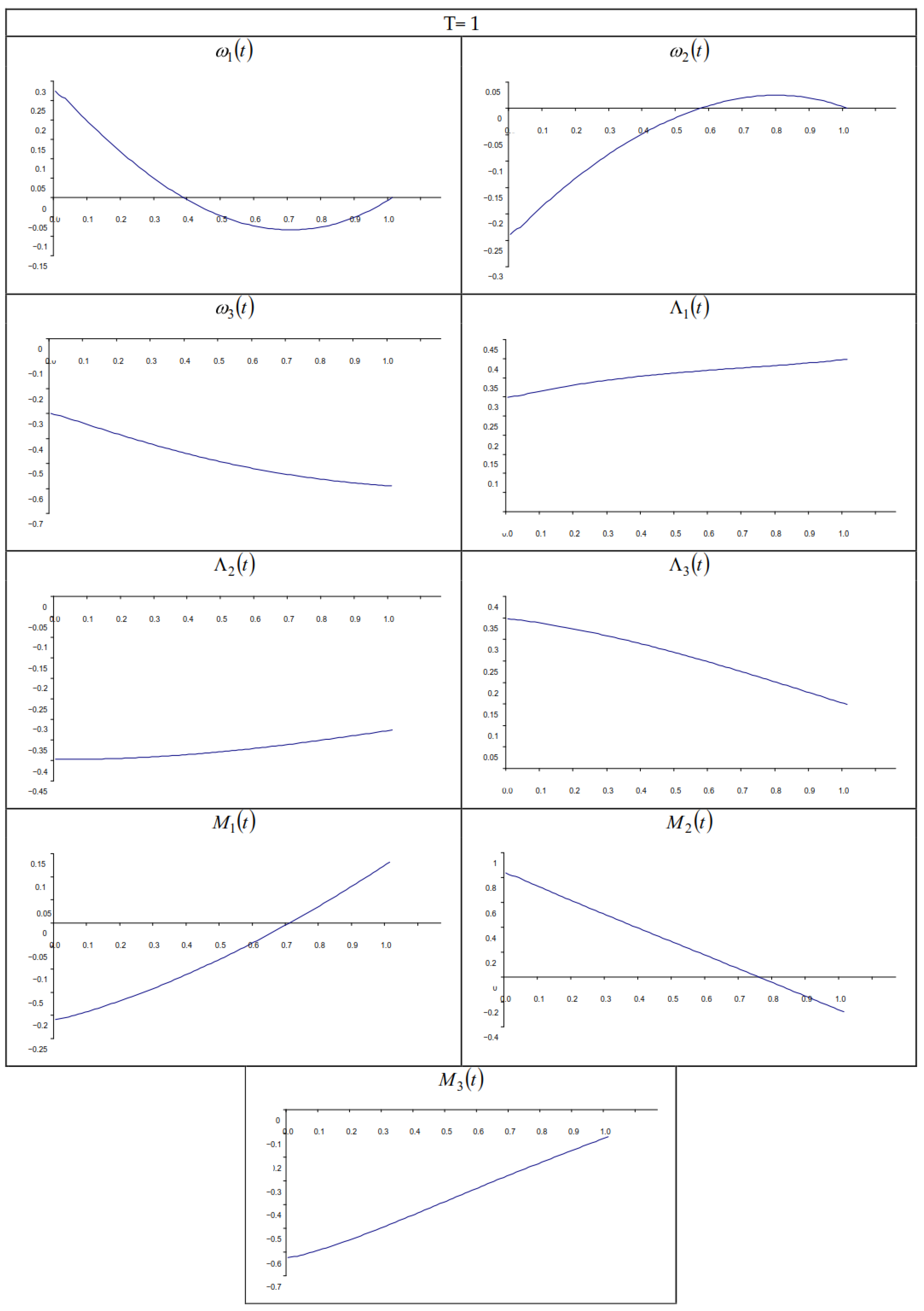
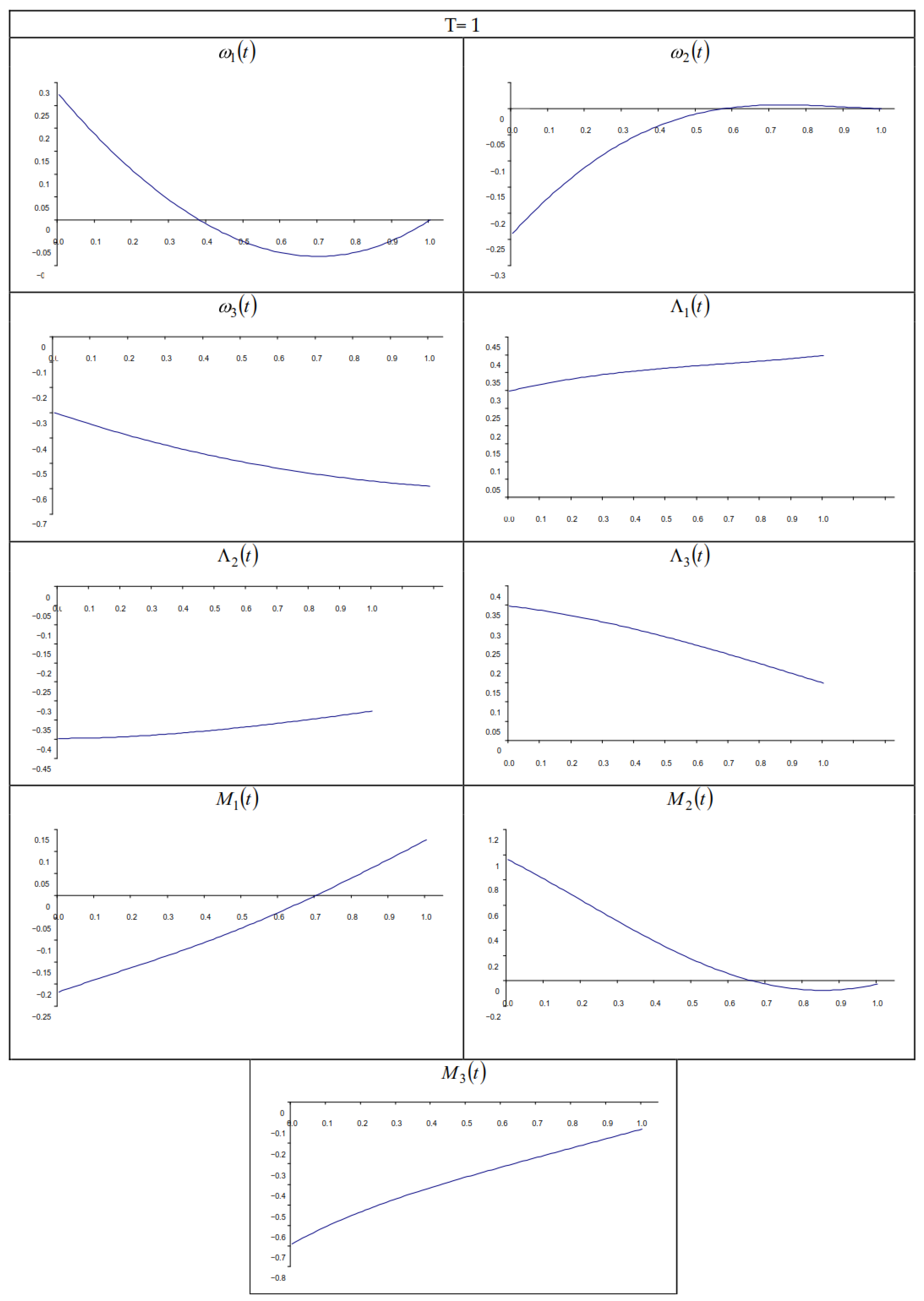
Below, for example, for Body4 (ISS), the graphs show the time variations of the angular velocity components ${\omega }_i(t), i= \overline{1,3},$ of the vector part of the orientation quaternion ${\mathsf{\Lambda }}_i(t), i= \overline{1,3}$, and of the components of the control moment $M_i^{}(t), i= \overline{1,3}$, in the classical optimal rotation problem (Figure 1) and in the modified control problem (Figure 2) for the arbitrary given boundary conditions (19) and (20). The curves ${\mathsf{\Lambda }}_1,{\mathsf{\Lambda }}_2, {\mathsf{\Lambda }}_3, {\omega }_1, {\omega }_2, {\omega }_3, M_1, M_3$ in the classical and modified problem for the ISS are similar and differ only for the components $M_2$ in both solutions.

From a large number of numerical calculations performed to solve the problem of a spacecraft optimal rotation with various boundary conditions and various main inertia moments $I_1, I_2, I_3$, the following conclusions can be made:

(1) Kinematic characteristics of the rotation of a spacecraft (attitude quaternion $\Lambda$ and angular velocity vector ($\mathsf{\omega }$) in the classical problem depend weakly on the mass distribution of a spacecraft and are mainly determined by the boundary conditions of the problem. For the modified problem, kinematic characteristics of the reorientation of a spacecraft depend only on the boundary conditions of the problem;

(2) The control moment significantly depends on a spacecraft’s main inertia moments and boundary conditions in both classical and modified formulations of the problem.

The weak dependence of kinematic characteristics of the optimal motion of a spacecraft on its dynamic configuration ensures the closeness of solutions for the modified and classical problems of the optimal rotation of a spacecraft with an arbitrary dynamic configuration. Therefore, the modified problem solution can be considered a quasioptimal solution of the classical spacecraft attitude problem.

Note that the spacecraft’s attitude quaternion $\Lambda (t)$ can have two values [2]: $\Lambda$ and $-\Lambda$ correspond to the same angular position of a spacecraft in space.

9. Conclusions

The analytical quasioptimal algorithm for controlling the angular motion of a spacecraft as a solid body of arbitrary dynamic configuration with arbitrary boundary conditions can be applied in spacecraft control systems. The proposed algorithm has a theoretical basis and solves the problem of optimal reorientation of a spacecraft with good accuracy. At the same time, it does not require a numerical solution of the boundary value problem of the maximum principle or any other complex numerical solution. The obtained results can be generalized to the cases of spacecraft control in the presence of flexible elements of spacecraft’s structure and various perturbations in the formulation of the problem. These results can also be applied to nano-class spacecrafts that have limitations on computing power.