The Optimization of a Model for Predicting the Remaining Useful Life and Fault Diagnosis of Landing Gear

Abstract

With the development of next-generation airplanes, the complexity of equipment has increased rapidly, and traditional maintenance solutions have become cost-intensive and time-consuming. Therefore, the main objective of this study is to adopt predictive maintenance techniques in daily maintenance in order to reduce manpower, time, and the cost of maintenance, as well as increase aircraft availability. The landing gear system is an important component of an aircraft. Wear and tear on the parts of the landing gear may result in oscillations during take-off and landing rolling and even affect the safety of the fuselage in severe cases. This study acquires vibration signals from the flight data recorder and uses prognostic and health management technology to evaluate the health indicators (HI) of the landing gear. The HI is used to monitor the health status and predict the remaining useful life (RUL). The RUL prediction model is optimized through hyperparameter optimization and using the random search algorithm. Using the RUL prediction model, the health status of the landing gear can be monitored, and adaptive maintenance can be carried out. After the optimization of the RUL prediction model, the root-mean-square errors of the three RUL prediction models, that is, the autoregressive model, Gaussian process regression, and the autoregressive integrated moving average, decreased by 45.69%, 55.18%, and 1.34%, respectively. In addition, the XGBoost algorithm is applied to simultaneously output multiple fault types. This model provides a more realistic representation of the actual conditions under which an aircraft might exhibit multiple faults. With an optimal fault diagnosis model, when an anomaly is detected in the landing gear, the faulty part can be quickly diagnosed, thus enabling faster and more adaptive maintenance. The optimized multi-fault diagnosis model proposed in this study achieves average accuracy, a precision rate, a recall rate, and an F1 score of more than 96.8% for twenty types of faults.

1. Introduction

The landing gear system is a critical component for the take-off and landing of aircrafts. Malfunctions in the landing gear system pose a serious risk to an aircraft’s take-off and landing operations and can potentially lead to significant casualties. With the advent of the jet age, the tricycle configuration of landing gear systems has been widely adopted. To enable steering, the structure of the front landing gear is designed differently from that of the rear landing gear, including the addition of steering brakes and steering linkages as transmission mechanisms to satisfy steering requirements.

Owing to the design requirements for steering, the stability of the front landing gear is relatively poor, making it susceptible to deviation and shimmy phenomena [1]. The front landing gear has the capability to steer left and right and interact with the elastic metal structure and the friction of the ground acting on the landing wheel. During the taxiing phase before take-off and after landing, external forces can affect the aircraft. When structural failure occurs, the front landing gear may deviate from its original direction of motion. Consequently, the interaction between the elastic structure and friction may lead to lateral shimmy phenomena, which occur perpendicular to the direction of motion.

If the rolling speed of the aircraft is low, this phenomenon gradually converges, resulting in the restoration of stability. However, as the speed increases to a certain value, this shimmy phenomenon becomes more pronounced, making it difficult to control the direction. This can lead to increased tire wear in the best case and to damage to the front fuselage structure and the landing gear system in the worst case, thus endangering flight safety [2].

This study focuses on the landing gear system, which, over a certain period of operation, is bound to exhibit anomalies. Therefore, it is essential to detect faulty components early before the landing gear’s malfunction can jeopardize aircraft safety or lead to damages. By doing so, maintenance time can be reduced, aircraft reliability can be enhanced, and maintenance efficiency can be improved. Research indicates that expenses associated with fleet operation and maintenance constitute 60–70% of the total lifecycle cost, while the increasing complexity of designs further contributes to the escalation of maintenance costs [3].

A functional health monitoring system for the shock absorber in landing gear was developed using prognostic and health management (PHM) [4]. The PHM-based landing gear system includes multiple sensors installed on the shock strut to monitor and record various shock absorber parameters, including gas temperature and pressure, and measure the stroke and travel of the shock absorber piston during an aircraft landing event. In addition, a PHM-based system can detect hard and heavy landings, enabling immediate maintenance action by staff.

Lee et al. proposed a cost-optimal RUL-driven maintenance strategy for the landing gear brakes of a fleet of aircraft [5]. Bayesian linear regression was used to predict the RUL of the brakes. Then, an integer linear program was used to combine all RUL predictions for the landing gear brakes of the fleet of aircraft. The results indicated that RUL-driven opportunistic maintenance led to 20% lower costs than traditional preventive maintenance.

Lin et al. focused on predictive maintenance of aircraft landing gear using a self-attention integrated learning model [6] and proposed multiple correlation analysis and a multilayer perception with the self-attention (MLPSA) method. First, three coefficients, including the Pearson coefficient, Spearman coefficient, and Kendall coefficient, were integrated to establish indicators that were used to select key features. Then, eight machine learning models, including Ridge, Elastic, KNN, SVM, DT, BP, RBF, and MLPSA, were used to predict the performance of the landing gear. The proposed MLPSA exhibited a smaller prediction error compared with other algorithms.

Hsu et al. [7] adopted the PHM methodology to construct a model for the prediction of remaining useful life (RUL) for landing gears. The health indicator (HI) was evaluated based on data acquired from the flight data recorder (FDR). Based on historical data from HI, the autoregressive integrated moving average (ARIMA) model was built to predict the lifetime of landing gear. However, there were significant discrepancies in the trends predicted using the three different forecasting algorithms. Furthermore, the specific components causing degradation in landing gear health remained unidentified.

Using the RUL prediction and fault diagnosis models, the status of the landing gear is time-varying, and the working conditions of the landing gear are non-stationary. Variations in missions, payload weights, weather conditions, and runway statuses can affect the degradation trend because the landing gear changes gradually. Additionally, the quality of the airport’s runway and the pilot’s driving technique affect the degradation trend. A model constructed in the present may not be suitable for the future.

To address this problem, we propose a practical application of the RUL prediction model and the fault diagnosis model constructed in the current study. Moreover, we focus on the hyperparameter optimization of algorithms to improve their predictive accuracy. In addition, a multi-fault diagnosis model is incorporated to facilitate the rapid maintenance and repair of faulty components. This approach is expected to reduce maintenance duration and increase aircraft reliability.

2. Problem Statement

2.1. Effects of Missing Data on the Prediction Model

In this study, we analyzed data collected from the flight data acquisition unit (FDAU). The FDAU gathers data from various sensors and avionic systems in the form of discrete, analog, and digital parameters. These parameters are then routed to the flight data recorder (FDR). We utilized historical data on take-offs and landings from each aircraft, along with associated maintenance records, which are downloaded monthly from the FDR by manufacturing and maintenance units. A total of 43 aircraft were included in the analysis. FDR data encompass parameters such as time, airspeed, and vibration, spanning a duration of approximately 10 years. The maintenance records comprise planned and unplanned maintenance activities.

The FDR begins to record data immediately after the engine starts. The recorded data cover all flight phases, including taxiing, take-off, climbing, cruising, descent, and landing. Given our focus is on landing gear, the data used for analysis pertain to aircraft operations on the ground, particularly during the high-speed taxiing phases of take-off and landing. To isolate the data during these high-speed taxiing phases, airspeed is used as an indicator. Since airspeed exhibits a monotonic increase before take-off and a monotonic decrease after landing, the airspeed can be utilized to filter out the high-speed taxiing data during take-off and landing.

However, owing to memory limitations within the FDR module, when extracting data from the FDR at scheduled intervals, a portion of the data can be overwritten and lost. Time intervals with missing data result in discontinuities. Missing data significantly affect the performance of the models. Thus, when predicting the RUL, it is essential to address the issue of missing values. The types of missing values can be classified as completely random, random, or nonrandom. There are two types of missing data: non-random missing values caused by data being overwritten because of insufficient memory, and completely random missing values that occur randomly and rarely. Techniques for handling missing values were used to mitigate the risk of prediction bias due to missing data [8].

2.2. Challenges to Identifying Different Fault Causes through Vibration Signals

Vibration signal analysis has emerged as a crucial tool for diagnosing and identifying various faults in mechanical systems. The methodology adopted in the current study uses vibration signals to discern distinct fault origins within these systems. By monitoring and analyzing vibration patterns, practitioners gain insights into the root causes of faults, enabling effective maintenance and troubleshooting.

To distinguish between different faults and the occurrence of multiple faults, it is necessary to examine historical maintenance records. These records encompass both planned and unplanned maintenance activities. As model construction requires maintenance actions associated with actual faults rather than those prompted by flight requirements, routine updates, or maintenance tasks, preprocessing of the maintenance record data involves filtering out maintenance actions related to actual faults. The initial step involves identifying maintenance actions related to real faults. Categorizing malfunctioning items based on vibration data requires the participation of domain experts possessing relevant expertise in this field.

3. Methodology

3.1. Basics of PHM Methodology

The PHM method was first applied in the field of aircraft maintenance [9]. The aim of PHM is to optimize operational readiness by employing affordable, integrated, and embedded diagnostics and prognostics, embedded training and testing, serialized item management, automatic identification technology (AIT), and iterative technology refreshes [10]. The PHM method has been widely applied in many industries, and many reviews of industrial applications have been published [11,12,13,14,15].

In the current study, the primary focus is on the use of the PHM method to perform health assessments, fault diagnosis, and RUL predictions for landing gear. The methodological flowchart of this study is shown in Figure 1. The analysis steps are as follows:

• First step: data acquisition;
• Second step: data preprocessing;
• Third step: feature extraction;
• Fourth step: feature selection;
• Last step: constructing a health assessment model, a fault diagnosis model, and an RUL model.

In the first step, the data acquired from the FDR must be filtered out of the taxiing data during take-off and landing before analysis. The dataset comprises information about the time, airspeed, y-axis vibration, and z-axis vibration acquired from the accelerometer sensor. The FDR records data from the initiation of aircraft engine start-up. The FDR data are not recorded at fixed intervals but rather when the signal exceeds the preset threshold value. To obtain the vibration data from the take-off and landing operations, the airspeed must be examined monotonically. The airspeed increases or decreases gradually for take-off or landing operation. Therefore, data filtering involves searching for a monotonically increasing airspeed for take-off data and a monotonically decreasing airspeed during take-off and landing operations.

The maintenance record form provides details of maintenance activities. We selected twenty items that are very important for landing gear maintenance. As shown in

Table 1. Twenty items used for the fault diagnosis model.

Item No.	Malfunctioning Item	Number of Data
A	Rose wheel/tire	224
B	Left main wheel/tire	947
C	Right main wheel/tire	899
D	Main wheel/tire	57
E	Main wheel hub	106
F	Nose wheel hub	77
G	Nose landing gear drag brace	25
H	Left landing gear drag brace	25
I	Right landing gear drag brace	41
J	Left landing gear brake	69
K	Right landing gear brake	61
L	Nose landing gear retract actuator	22
M	Left landing gear retract actuator	24
N	Right landing gear retract actuator	27
O	Nose landing gear shock strut	37
P	Left landing gear shock strut	37
Q	Right landing gear shock strut	40
R	Steering actuator	27
S	Steering control valve	5
T	Brake control valve	26
Total		2776

, the faulty items are 1. nose wheel/tire; 2. left main wheel/tire; 3. right main wheel/tire; 4. main wheel/tire; 5. main wheel hub; 6. nose wheel hub; 7. nose landing gear drag brace; 8. left landing gear drag brace; 9. right landing gear drag brace; 10. left landing gear brake; 11. right landing gear brake; 12. nose landing gear retract actuator; 13. left landing gear retract actuator; 14. right landing gear retract actuator; 15. nose landing gear shock strut; 16. left landing gear shock strut; 17. right landing gear shock strut; 18. steering actuator; 19. steering control valve; and 20. brake control valve. Based on our observations, it is imperative to determine the main malfunctioning items in current maintenance activities and properly document them. However, when the maintenance record form indicates the occurrence of more than one malfunctioning item, that is, multiple faults occurring simultaneously, the multi-fault label method is required [16]. We employ the one-hot encoding technique to ensure that multiple faults can be distinguished by the classification algorithms. Figure 2 shows the utilization of the one-hot encoding method to reencode multiple items from the maintenance record form.

We extracted ten time-domain features, such as peak-to-peak, mean, root mean square, standard deviation, skewness, kurtosis, crest indicator, clearance indicator, shape indicator, and impulse indicator, from the signals. The definitions of these characteristics can be found in our previous work [7].

This study adopted a wrapper approach based on Fisher’s criterion for feature selection, as proposed in the literature [17]. After selecting the crucial features, a logistic regression algorithm was adopted to calculate the HI from historical data. After the HI was evaluated, the RUL prediction model can be implemented using various algorithms. In the previous study [7], we adopted the ARIMA algorithm to predict the RUL of the landing gear. In the current study, we adopted more algorithms to obtain more accurate predictions and compare their performances. Therefore, time-series analysis techniques, such as the autoregressive model (AR) [18], ARIMA model [19], and Gaussian process regression (GPR) model [20], were used to implement the prediction model for landing gear. The AR model offers advantages such as simplicity and efficiency, making it suitable for short-term forecasting. The ARIMA model can handle trends and seasonality, offering greater flexibility. The GPR model has the characteristics of a non-parametric regression method, meaning that it can capture complex, non-linear relationships in time-series data. In addition, GPR can handle irregularly spaced data points and is well-suited for data with nonuniform sampling intervals. Obviously, GPR has a considerably greater advantage in handling landing gear datasets. To improve model accuracy, a monotonicity check was performed to ensure a monotonous degradation of the HI while predicting RUL. The re-ranking of features was also performed based on the monotonicity check [7,16].

In this study, we employed the XGBoost (eXtreme Gradient Boost) algorithm for fault classification modeling [21,22]. The XGBoost algorithm is based on the gradient-boosted decision tree (GBDT) and encompasses the advantages of both bagging and boosting, representing an enhanced algorithm. One of its primary strengths is the ability to amalgamate weak classifiers into a strong classifier. This algorithm is particularly beneficial for developing diagnostic models for the multi-fault classification model. We adopted the crucial features of these twenty fault types and the multi-fault labels obtained from the one-hot encoding technique for fault codes into the classification model.

3.2. Hyperparameter Optimization

3.2.1. Optimization of the RUL Model

The performance of many machine learning algorithms depends on their hyperparameter settings. Therefore, to achieve optimal accuracy of the prediction model, hyperparameter optimization was applied. However, defining a formula to discover the optimal hyperparameters is challenging. Some optimization strategies, such as manual search, grid search, random search, and Bayesian optimization, have been proposed [18,19,20,21,22,23]. In the current study, random search was used for RUL model optimization. As shown in Figure 3, different combinations of varying hyperparameters were used to train the AR, ARIMA, and GPR predictive models, and the corresponding model performances were evaluated using a loss function. Through a continuous search, our objective was to minimize the loss function, thereby obtaining the optimal RUL prediction model.

The objective of hyperparameter optimization is to find an optimal setting of the hyperparameters of the AR, ARIMA, and GPR algorithms as quickly as possible. As previously mentioned, due to the varying flight tasks, distinct operational conditions, and random absence of historical data, the optimal hyperparameters for each aircraft differ. Therefore, optimizing these hyperparameters is essential to ensure that each aircraft has the best RUL prediction model. However, given the algorithms used here, i.e., AR, ARIMA, and GPR, the number of hyperparameters, their value ranges, and their significance vary. In this context, we employ a random search method for hyperparameter optimization. Compared to grid search and manual search, random search can find superior models by effectively searching for a larger but less promising configuration space in the same domain [24,25]. As shown in Algorithm 1: random search optimization, a pseudo code for random search optimization, is employed.

As detailed in Algorithm 1, the initial settings of the random search optimization algorithm are established. This includes the initialization of the model score, denoted as ‘best_score’; the maximum number of iterations, termed ‘iterations’; the hyperparameter space, term ‘hyperparameter_space’; and the model to be optimized. Following these settings, the optimization process begins. For each iteration, hyperparameters are randomly selected from the hyperparameter space and then integrated into the model. Cross-validation is used for model evaluation. If the current model’s evaluation score surpasses the initial best_score, then the best_hyperparameters are replaced by the present hyperparameters. This iterative process continues until the best hyperparameters are determined. The hyperparameters used for optimization in the AR, ARIMA, and GPR algorithms are shown in

Table 2. Hyperparameters used in the AR algorithm [26].

No	Hyperparameter	Search Range	Description
1	P	Integer (0–10)	Number of previous time steps.

,

Table 3. Hyperparameters used in the ARIMA algorithm [26].

No	Hyperparameter	Search Range	Description
1	P	Integer (0–10)	Number of previous time steps.
2	D	Integer (0–5)	Number of times differencing.
3	Q	Integer (0–10)	Number of previous forecast errors.

and

Table 4. Hyperparameters used in the GPR algorithm.

No	Hyperparameter	Search Range	Description
1	Kernel	Categorical (‘kernel_rbf’, ‘kernel_rq’, ‘kernel_expsine’, ‘kernel_matern’, ‘kernel_dotproduct’)	Kernel specifying the covariance function of the Gaussian process.
2	Alpha	Integer ($1\times {10}^{-13}$ $1\times {10}^{-12}$, $1\times {10}^{-11}$, $1\times {10}^{-10}$, $1\times {10}^{-9}$, $1\times {10}^{-8}$,$1\times {10}^{-7}$)	Value added to the diagonal of the kernel matrix during fitting.
3	n_restarts_optimizer	Integer (0, 1, 2, 3)	Number of restarts of the optimizer for finding the kernel parameters that maximize the log-marginal likelihood.

, respectively. The parameters are detailed on the Statsmodels website [26].

Algorithm 1: Random Search Optimization

function RandomSearch(model, hyperparameter_space, iterations):

best_score = 0

for i = 1 to iterations do:

sampled_hyperparameters = SampleFrom(hyperparameter_space)

current_model = TrainModel(model, sampled_hyperparameters)

current_score = Evaluate(current_model)

if current_score > best_score:

best_score = current_score

best_hyperparameters = sampled_hyperparameters

return best_hyperparameters

3.2.2. Optimization of the Fault Diagnosis Model

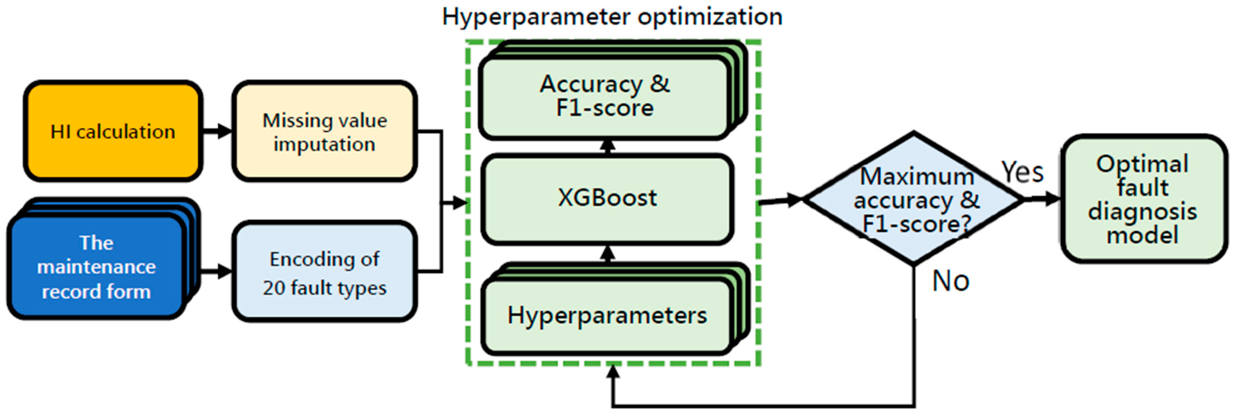
In the implementation of the multi-fault diagnosis model, in addition to using the HI corresponding to each fault repair event, it is essential to incorporate the fault category occurring in each maintenance activity, as represented by fault codes, into the classification model. Subsequently, we calculated the accuracy and F1 score of the classification model, introduced various hyperparameters, and recorded the corresponding accuracy and F1 score. Through iterative refinements aimed at maximizing the model’s accuracy and F1 score, we can derive the optimal fault diagnosis model. The classification algorithm, such as XGBoost [17,18,19,20], was used to construct the fault diagnosis model in conjunction with the one-hot encoding method. Figure 4 shows the flowchart of the optimization process. Hyperparameter optimization was applied to enhance model performance using a random search algorithm [26,27,28,29,30,31,32]. We used the Python code to develop the program for XGBoost hyperparameter tuning [32].

The fundamental concept of Bayesian optimization involves using past samples of the objective function, f, to determine the next optimal point for sampling, f. The Gaussian process is a convenient and powerful prior distribution on functions f. We assume that the function f(x) is drawn from a Gaussian process prior, and our observations are in the form $f_{\varphi }\left(x\right)$. The optimization problem can be defined as Equation (1), and the key steps of the Bayesian optimization algorithm are outlined in Algorithm 2:

$${\varnothing }^{*}=arg\begin{array}{c}\\ max\\ \varnothing \in \mathsf{\Phi }\end{array}{f}_{\varphi }(x),$$

(1)

where $\mathsf{\Phi }$ is the space of all possible hyperparameters, and ${\varnothing }^{*}$ is the current best-observed outcome by $\varnothing \in \mathsf{\Phi }$. The hyperparameters used for optimization in the XGBoost algorithms are shown in

Table 5. Hyperparameters used in the XGBoost algorithm [21].

No	Hyperparameter	Search Range	Description
1	n_estimators	Integer (100–10,000)	Number of boosting rounds.
2	max_depth	Integer (100–10,000)	Maximum tree depth for base learners.
3	learning_rate	Real number (0.01–0.5)	Boosting learning rate.
4	Booster	Categorical (‘gbtree’, ‘dart’)	Specify which booster to use: gbtree, gblinear, or dart.
5	Gamma	Real number (0–1000)	Minimum loss reduction required to make a further partition on a leaf node of the tree.
6	min_child_weight	Real number (1–100)	Minimum sum of instance weight (hessian) needed in a child.
7	Subsample	Real number (0.5–1)	Subsample ratio of the training instance.
8	colsample_bytree	Real number (0.5–1)	Subsample ratio of columns when constructing each tree.
9	reg_alpha	Real number (0–1)	L1 regularization term on weights.
10	reg_lambda	Real number (0–1)	L2 regularization term on weights.

[24].

Algorithm 2: Bayesian Optimization

Function BayesianOptimization(model, hyperparameter_space, evaluations):

Initialize an empty dataset D to store hyperparameters and their respective scores     for i = 1 to evaluations do:         surrogate_model = Fit(D)         next_hyperparameters = SelectNext(surrogate_model, hyperparameter_space)         new_score = Evaluate(model, next_hyperparameters)         new_data_point = (next_hyperparameters, new_score)         Add new_data_point to D     best_hyperparameters = hyperparameters in D with the highest score     return best_hyperparameters

The metric used for the evaluation of the RUL prediction model is the loss function. The loss function, also known as the cost function, serves as a measure to evaluate the discrepancy between the predicted and actual values. A smaller loss function indicates a closer alignment of the model’s predictions with the actual values, signifying a more robust model. Common regression loss functions are represented as root-mean-square error (RMSE), as shown by the following:

$$\mathrm{R}\mathrm{M}\mathrm{S}\mathrm{E}=\sqrt{\frac{1}{n}{\sum }_{i=1}^n{\left({y_i-\widehat{y}}_i\right)}^2},$$

(2)

where ${\widehat{y}}_i$ is a predicted value, $y_i$ is an actual value, and $n$ is the number of data. Our goal is to minimize the RMSE during hyperparameter optimization.

In terms of the fault diagnosis model, the metrics used for evaluation are accuracy, recall rate, precision rate, and F1 score, as shown by the following:

$$\mathrm{A}\mathrm{c}\mathrm{c}\mathrm{u}\mathrm{r}\mathrm{a}\mathrm{c}\mathrm{y}=\frac{TP+TN}{TP+FP+FN+TN},$$

(3)

$$\mathrm{P}\mathrm{r}\mathrm{e}\mathrm{c}\mathrm{i}\mathrm{s}\mathrm{i}\mathrm{o}\mathrm{n} \mathrm{r}\mathrm{a}\mathrm{t}\mathrm{e}=\frac{TP}{TP+FP},$$

(4)

$$\mathrm{R}\mathrm{e}\mathrm{c}\mathrm{a}\mathrm{l}\mathrm{l} \mathrm{r}\mathrm{a}\mathrm{t}\mathrm{e}=\frac{TP}{TP+FN},\mathrm{and}$$

(5)

$$\mathrm{F}1 \mathrm{s}\mathrm{c}\mathrm{o}\mathrm{r}\mathrm{e}=\frac{2\times \mathrm{P}\mathrm{r}\mathrm{e}\mathrm{s}\mathrm{i}\mathrm{o}\mathrm{n} \mathrm{r}\mathrm{a}\mathrm{t}\mathrm{e}\times \mathrm{R}\mathrm{e}\mathrm{c}\mathrm{a}\mathrm{l}\mathrm{l} \mathrm{r}\mathrm{a}\mathrm{t}\mathrm{e}}{\mathrm{P}\mathrm{r}\mathrm{e}\mathrm{s}\mathrm{i}\mathrm{o}\mathrm{n} \mathrm{r}\mathrm{a}\mathrm{t}\mathrm{e}+\mathrm{R}\mathrm{e}\mathrm{c}\mathrm{a}\mathrm{l}\mathrm{l} \mathrm{r}\mathrm{a}\mathrm{t}\mathrm{e}}.$$

(6)

where TP denotes true positives, TN denotes true negatives, FP denotes false positives, and FN denotes false negatives in the confusion matrix. To avoid the overfitting of the model, a ten-fold cross-validation scheme was used for the evaluation of model performance. The primary objective is to maximize accuracy, recall rate, precision rate, and the F1 score during hyperparameter optimization.

4. Results and Discussion

4.1. Health Indicator Model

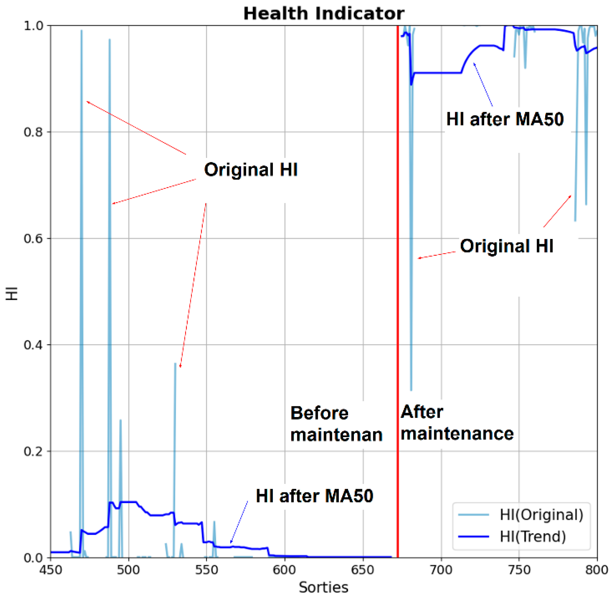
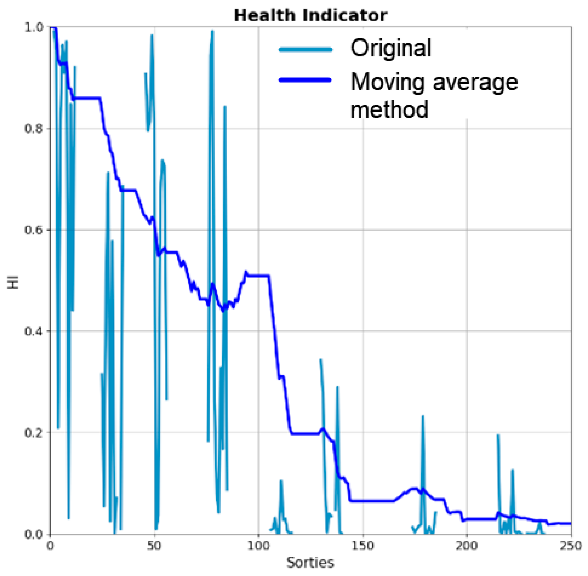
By defining the state before and after maintenance and inputting key features into the health assessment module, the HIs of each aircraft landing gear can be calculated, as shown in Figure 5. However, because of the limited memory capacity of older FDRs, the data from some flights are missing. Therefore, a moving average method [26] with a window size of 50 flights (MA50) was used to estimate the missing values, thus obtaining a complete HI curve. We used the moving average window to not only tackle the issue of data discontinuity but also eliminate the severe fluctuation of the HIs. In order to determine the proper window size, we varied it from 0 to 100. Based on the current data, we selected a window size of 50 for the best results. The health status of each airplane is indicated by its HI. Any fault in the items listed in Table 1 can degrade that item’s HI. Based on historical HIs, we can predict the future trend of His by using the regression algorithm and identify the faulty item using the classification algorithm.

4.2. RUL Prediction Model

After obtaining the full HI curve of each aircraft’s landing gear from the HI model, we can implement the RUL prediction model. As shown in Figure 6, the original HI, as calculated from the HI model, is not continuous, which is attributed to the insufficient memory of the aircraft itself. Additionally, the pronounced fluctuations in the HI can be ascribed to the variations in the flights, payload weights, weather conditions, and runway statuses of each flight. To construct an RUL prediction model, we must address discontinuities within the HI. To this end, we employ a moving average method with a window size of 50 (MA50) to address the issue of data discontinuity. After processing, we obtain a continuous HI curve, as shown in Figure 6. Based on the HI curve, we can then construct the RUL prediction model.

The RUL prediction models were implemented using the AR, ARIMA, and GPR algorithms. A certain period of historical HI data was used to train the prediction model. For a prediction made at arbitrary time A, the historical HI data before time A were used as training data, and the historical HA data after time A were used as testing data. The results of the three RUL prediction models, i.e., AR, ARIMA, and GPR algorithms, are compared in Figure 7. The performances of the RUL prediction model were evaluated from the testing data and the prediction data calculated from AR, ARIMA, and GPR.

As discussed in the Introduction, the status of a landing gear is time-varying, and its working conditions are nonstationary. The flights, payload weights, weather conditions, pilot’s operational habits, and the distance and condition of the runway may affect the degradation trend. Therefore, in the current study, we first determine the HI using key features. Then, we can use the historical HI to predict the future degradation trend. Thus, to make predictions on time A, we can use the historical HI shortly before time A to predict the future trend from time A. The prediction is more precise if the future trend from time A is affected directly by the historical HI shortly before time A.

4.3. Optimization of the RUL Prediction Model

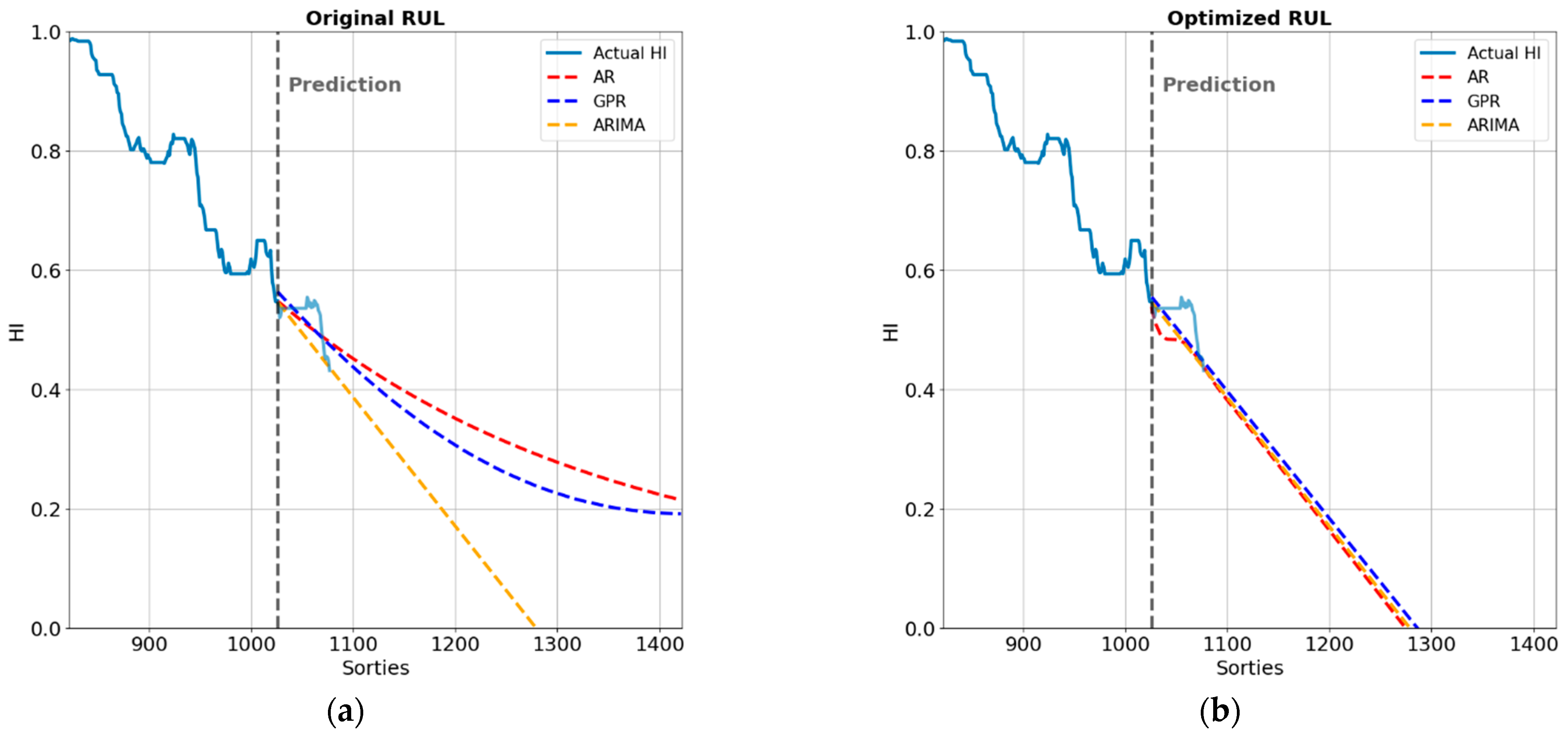
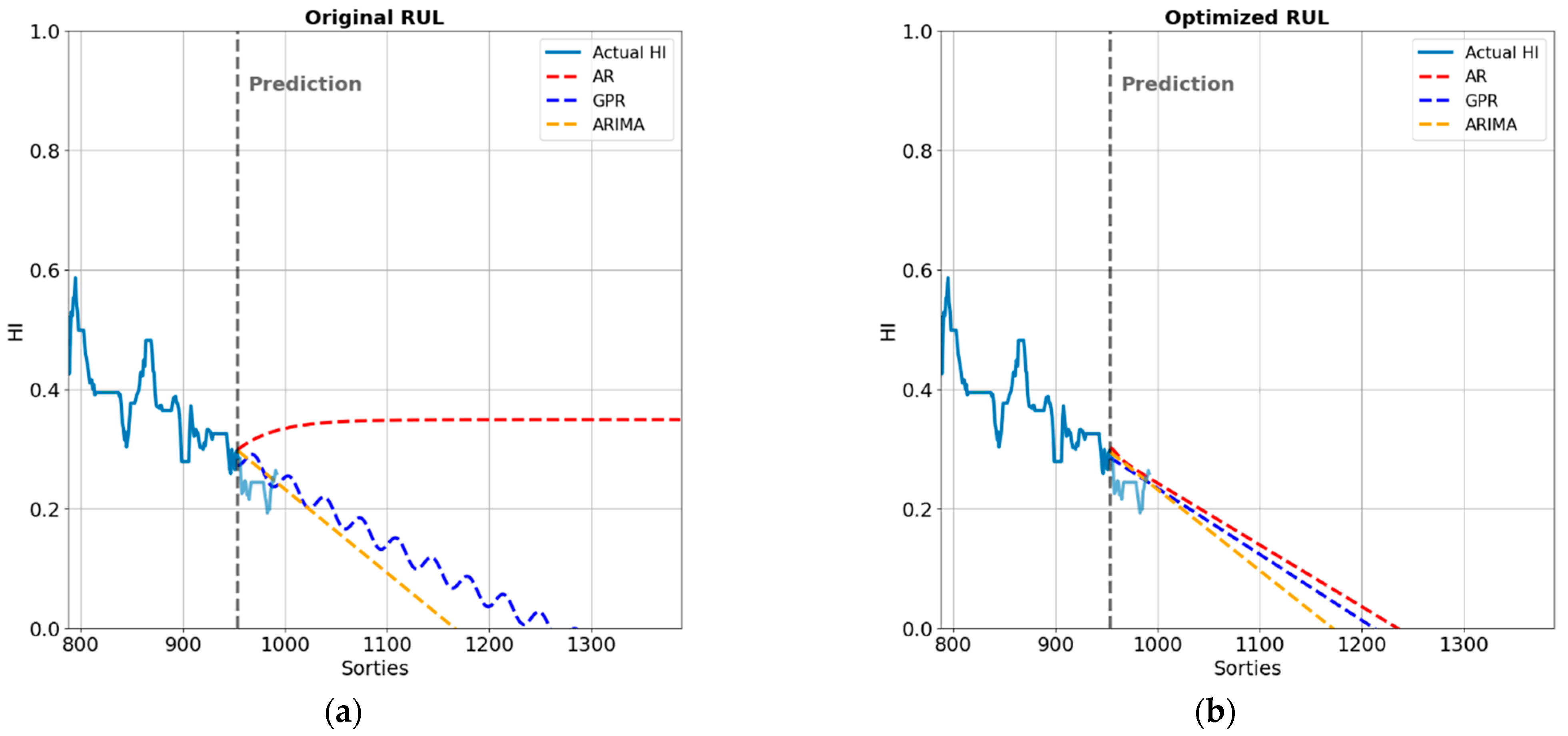
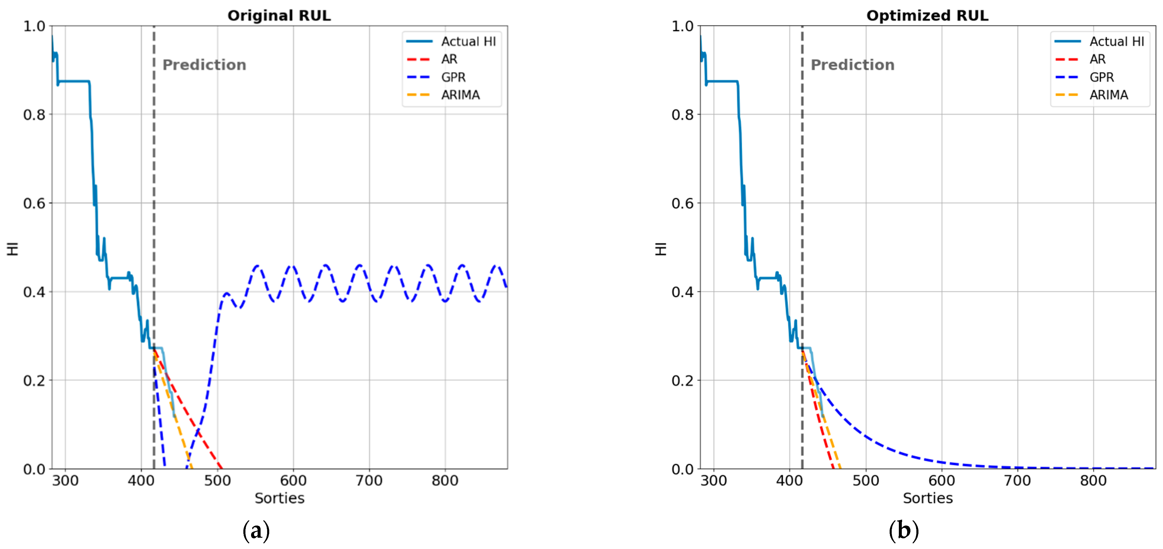
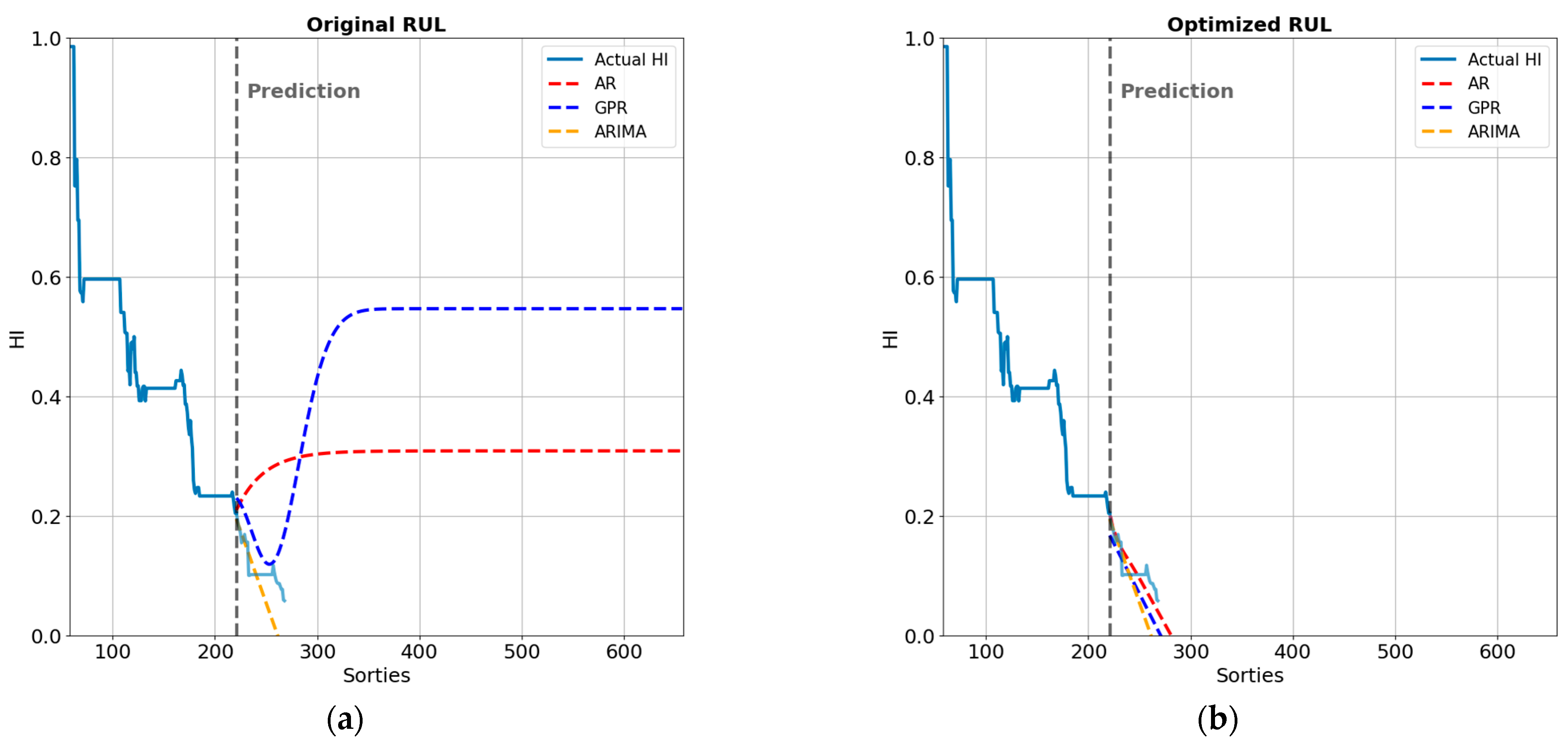
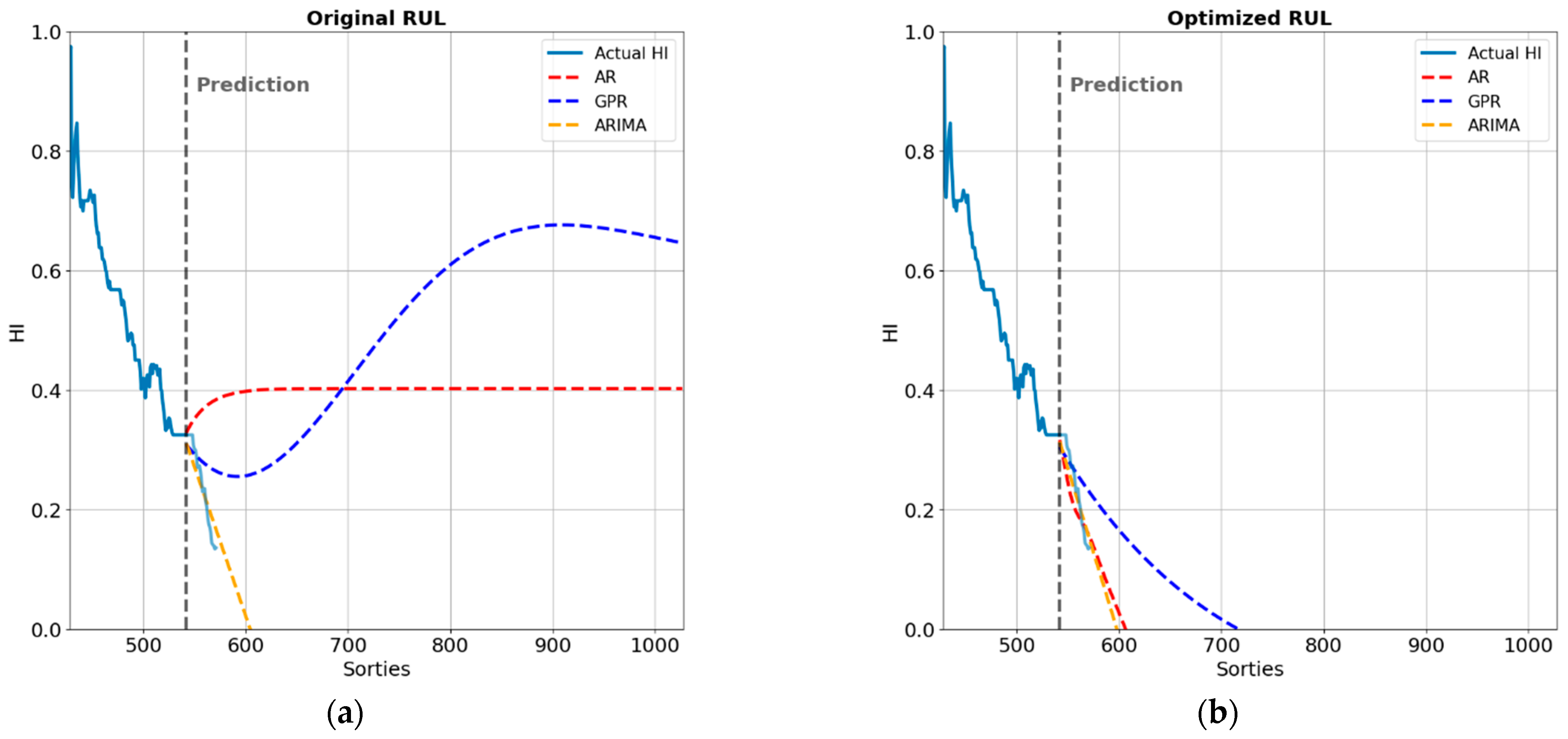
To optimize the RUL prediction model, the first 80% of the historical data for each airplane was used as training data, while the remaining 20% was used as validation data. Seven airplanes were selected for hyperparameter optimization.

Table 6. Comparison of the results of the RUL prediction model with AR before and after optimization.

Airplane Number	Optimization	Actual HI of Latest Flight	Predicted HI of Latest Flight	RMSE	Error Range
Airplane #1	Before	0.379	0.391	0.013	[−0.017, 0.026]
	After	0.379	0.358	0.022	[0.000, 0.047]
Airplane #2	Before	0.718	0.712	0.026	[−0.081, 0.010]
	After	0.718	0.685	0.030	[−0.045, 0.048]
Airplane #3	Before	0.431	0.479	0.027	[−0.048, 0.050]
	After	0.431	0.436	0.050	[−0.005, 0.071]
Airplane #4	Before	0.259	0.331	0.082	[−0.133, 0.014]
	After	0.259	0.251	0.040	[−0.071, 0.012]
Airplane #5	Before	0.117	0.176	0.028	[−0.062, 0.039]
	After	0.117	0.077	0.056	[−0.007, 0.081]
Airplane #6	Before	0.058	0.291	0.157	[−0.233, −0.006]
	After	0.058	0.040	0.022	[−0.043, 0.043]
Airplane #7	Before	0.136	0.384	0.145	[−0.249, −0.003]
	After	0.136	0.155	0.040	[−0.027, 0.063]
Average	Before			0.0682
	After			0.0371

,

Table 7. Comparison of the results of the RUL prediction model with ARIMA before and after optimization.

Airplane Number	Optimization	Actual HI of Latest Flight	Predicted HI of Latest Flight	RMSE	Error Range
Airplane #1	Before	0.379	0.340	0.038	[0.005, 0.065]
	After	0.379	0.342	0.036	[0.004, 0.064]
Airplane #2	Before	0.718	0.677	0.024	[−0.050, 0.044]
	After	0.718	0.677	0.024	[−0.050, 0.044]
Airplane #3	Before	0.431	0.436	0.043	[−0.022, 0.081]
	After	0.431	0.435	0.044	[−0.021, 0.081]
Airplane #4	Before	0.259	0.244	0.038	[−0.066, 0.019]
	After	0.259	0.243	0.037	[−0.064, 0.020]
Airplane #5	Before	0.117	0.120	0.037	[−0.008, 0.063]
	After	0.117	0.120	0.037	[−0.008, 0.063]
Airplane #6	Before	0.058	−0.032	0.054	[−0.037, 0.100]
	After	0.058	−0.032	0.054	[−0.036, 0.100]
Airplane #7	Before	0.136	0.167	0.027	[−0.044, 0.043]
	After	0.136	0.151	0.025	[−0.030, 0.045]
Average	Before			0.0372
	After			0.0367

and

Table 8. Comparison of the results of the RUL prediction model with GPR before and after optimization.

Airplane Number	Optimization	Actual HI of Latest Flight	Predicted HI of Latest Flight	RMSE	Error Range
Airplane #1	Before	0.379	0.704	0.163	[−0.325, −0.002]
	After	0.379	0.314	0.063	[0.024, 0.094]
Airplane #2	Before	0.718	0.771	0.068	[−0.136, −0.043]
	After	0.718	0.707	0.027	[−0.080, 0.014]
Airplane #3	Before	0.431	0.474	0.027	[−0.043, 0.050]
	After	0.431	0.446	0.037	[−0.030, 0.071]
Airplane #4	Before	0.259	0.238	0.039	[−0.073, 0.027]
	After	0.259	0.243	0.032	[−0.060, 0.020]
Airplane #5	Before	0.117	−0.107	0.206	[0.043, 0.268]
	After	0.117	0.173	0.031	[−0.058, 0.049]
Airplane #6	Before	0.058	0.171	0.051	[−0.113, −0.005]
	After	0.058	0.009	0.037	[−0.027, 0.071]
Airplane #7	Before	0.136	0.264	0.068	[−0.131, 0.029]
	After	0.058	0.009	0.037	[−0.027, 0.071]
Average	Before			0.0888
	After			0.0398

display the prediction results for each model, comprising actual and predicted values of the final airplane’s health index, RMSE, and error range. Based on the model evaluation outcomes, the RMSE error was consistently lower than 0.1 after hyperparameter optimization. The average RMSE error for the AR model decreased from 0.0682 to 0.0371, representing a reduction of 45.69%. The ARIMA model’s average RMSE error decreased from 0.0372 to 0.0367, which is a slight reduction of 1.34%. For GPR, the average RMSE error decreased from 0.0888 to 0.0398, which is a reduction of 55.18%. The results of this study indicate that optimized prediction outcomes are more accurate than before optimization, with significant reductions in RMSE errors observed for both AR and GPR models.

Figure 8, Figure 9, Figure 10, Figure 11, Figure 12, Figure 13 and Figure 14 compare the three algorithms—AR, ARIMA and GPR—before and after hyperparameter optimization. As illustrated in the figures, after hyperparameter optimization, the trend of the HI prediction curve becomes more reasonable, aligning with the gradually declining trend of HI. Conversely, before optimization, the HI prediction trend occasionally exhibits sudden increases, which clearly deviate from the actual scenario. In addition, the consistency of the predictions for the seven airplanes from the three algorithms varied before optimization. However, after the optimization process, the predictions become more aligned, indicating that optimization significantly enhances the accuracy of predictions, thus greatly improving the practicality of the models.

4.4. Optimization of the Fault Diagnosis Model

We extracted 15,706 data entries from the FDR. However, because of overwriting issues in the FDR, only 2776 data entries could be used for labeling as faulty items. The total numbers of each faulty item are provided in

Table 9. Results of the fault diagnosis model after hyperparameter optimization.

Item	Malfunctioning Item	Accuracy	Precision Rate	Recall Rate	F1 Score
A	Nose wheel/tire	99.96%	100.00%	96.88%	98.41%
B	Left main wheel/tire	99.73%	100.00%	95.56%	97.73%
C	Right main wheel/tire	99.80%	100.00%	96.44%	98.19%
D	Main wheel/tire	99.97%	100.00%	91.23%	95.41%
E	Main wheel hub	99.95%	100.00%	92.45%	96.08%
F	Nose wheel hub	99.97%	100.00%	93.51%	96.64%
G	Nose landing gear drag brace	99.99%	100.00%	96.00%	97.96%
H	Left landing gear drag brace	100.0%	100.00%	100.00%	100.00%
I	Right landing gear drag brace	100.0%	100.00%	100.00%	100.00%
J	Left landing gear brake	99.98%	100.00%	95.45%	97.67%
K	Right landing gear brake	99.98%	100.00%	95.08%	97.48%
L	Nose landing gear retract actuator	100.00%	100.00%	100.00%	100.00%
M	Left landing gear retract actuator	100.00%	100.00%	100.00%	100.00%
N	Right landing gear retract actuator	99.99%	100.00%	96.30%	98.11%
O	Nose landing gear shock strut	99.99%	100.00%	97.30%	98.63%
P	Left landing gear shock strut	100.00%	100.00%	100.00%	100.00%
Q	Right landing gear shock strut	99.99%	100.00%	97.50%	98.73%
R	Steering actuator	100.00%	100.00%	100.00%	100.00%
S	Steering control valve	100.00%	100.00%	100.00%	100.00%
T	Brake control valve	99.99%	100.00%	92.31%	96.00%
Average		99.96%	100.00%	96.80%	98.35%

. During hyperparameter optimization, we employed cross-validation to validate the performance of our proposed model. The evaluation results for the accuracy, precision rate, recall rate, and F1 score of the twenty fault types are displayed in Table 9. As shown in the table, the optimized model achieved an average accuracy rate of higher than 96% in detecting faults in the landing gear components, indicating that this optimized fault diagnosis model is applicable in practice.

We can see that the fault diagnosis model achieved 100% accuracy for some malfunctioning items. As discussed in the Methodology section, ten time-domain features were extracted from four signal data, i.e., take-off y-axis vibration, take-off z-axis vibration, landing y-axis vibration, and landing z-axis vibration. A total of forty features were used for the XGBoost algorithm. In addition, we adopted the one-hot encoding technique in conjunction with the XGBoost algorithm. The multi-fault classification model can simultaneously output multiple fault types. The results showed that some items related directly to vibration correspond to notably high accuracy, for example, the left landing gear drag brace, the right landing gear drag brace, the nose landing gear retract actuator, the steering actuator, and the steering control valve. Some other items, such as brakes or shock struts, yield lower accuracy.

To evaluate the statistical significance of the fault diagnostic model’s results, we used the ten-fold cross-validation method to obtain ten accuracies with the XGBoost algorithm. Then, we used a one-sample t-test to test the significance of the model. The results showed that the classifier of the fault diagnostic model is significant (p-value < 0.05) [33].

4.5. Applications of RUL Prediction Model and the Fault Diagnosis Model

Figure 15 shows the thresholds for two HI levels confirmed by experts, that is, HI = 0.65 and HI = 0.2. The HI can be divided into three regions: the white region (1.0 < HI < 0.65) indicates a healthy status, the yellow region (0.65 < HI < 0.2) indicates a degraded state, and the red region (0.65 < HI < 0.2) indicates a critical state. We predict the future trend of the HI from point A, as shown in Figure 15. If the predicted HI of the landing gear falls into the critical state, then maintenance service can be arranged for the plane before failure occurs. Predictive maintenance can be achieved using the RUL prediction model.

To confirm what kind of fault type occurs when the HI decreases, we can input the feature dataset of the flights. The fault diagnosis model proposes the fault type. The maintenance engineer can perform maintenance according to the suggestions and thus reduce the mean time to repair (MTTR) and increase the availability rate.

5. Conclusions

Previous researchers predicted the remaining useful life (RUL) of landing gear using a model with a fixed set of hyperparameters. When various aircrafts exhibited different trends of degradation because of a multitude of factors, this approach led to substantial discrepancies in the prediction accuracy. According to the results of this study, the root-mean-square (RMSE) errors after hyperparameter optimization in all cases were less than 0.1. The RMSE errors for the three algorithms were 0.0371, 0.0398, and 0.0367, respectively, all of which outperformed previous research [7].

To address the issue of accuracy variations due to different degradation trends and more accurately reflect the actual conditions of each aircraft’s landing gear, this study considered factors such as the pilot’s operational habits, length and conditions of the runway, and meteorological conditions, which contribute to different degradation patterns. Hyperparameter optimization techniques were implemented, achieving RMSE errors consistently less than 0.1 after optimization. After hyperparameter optimization, the average RMSE errors for the autoregressive model (AR), autoregressive integrated moving average (ARIMA), and Gaussian process regression (GPR) models decreased by 45.69%, 1.34%, and 55.18%, respectively. These results confirm that hyperparameter optimization effectively improves prediction accuracy and captures the diverse degradation patterns of landing gears.

In the current study, we adopted the one-hot encoding technique to overcome the inability to simultaneously output multiple types of faults. In conjunction with the XGBoost algorithm, the multi-fault classification model can simultaneously output multiple fault types. This model more realistically represents conditions where an aircraft might exhibit multiple faults that are not mutually exclusive. By using XGBoost for multilabel classification and incorporating records from various operational conditions, the model distinguished between twenty different fault types, achieving an average accuracy of 99.96%. According to the findings of this study, the fault diagnosis module achieved an average precision, precision rate, recall rate, and F1 score of 99.96%, 100.00%, 96.80%, and 98.35%, respectively. This confirms that the XGBoost model can be used to diagnose multiple fault types simultaneously with high accuracy.

This study demonstrated that, even with data limitations, reliable results can be achieved for aircraft in their mid-to-late service life using prognostic and health management techniques. The empirical results of this study also support the application of data-driven methods to complement traditional reliability engineering based on experiential judgments in fleet maintenance management.

References

1. Lernbeiss, R.; Plöchl, M. Simulation Model of an Aircraft Landing Gear Considering Elastic Properties of the Shock Absorber. Proc. Inst. Mech. Eng. Part K J. Multi-Body Dyn. 2007, 221, 77–86. [Google Scholar] [CrossRef]
2. Currey, N.S. Aircraft Landing Gear Design: Principles and Practices; AIAA Education Series; American Institute of Aeronautics and Astronautics, Inc.: Reston, VA, USA, 1988; Available online: https://arc.aiaa.org/doi/book/10.2514/4.861468 (accessed on 25 October 2023).
3. Czaban, M. Aircraft Corrosion—Review of Corrosion Processes and Its Effects in Selected Cases. Fatigue Aircr. Struct. 2018, 2018, 5–20. [Google Scholar] [CrossRef]
4. Haider, S. Overview of prognostics and health management for landing gear maintenance. In Proceedings of the 2019 Annual Reliability and Maintainability Symposium (RAMS), Orlando, FL, USA, 28–31 January 2019; IEEE: New York, NY, USA, 2019; pp. 1–7. [Google Scholar]
5. Lee, J.; Pater, I.; Boekweit, S.; Mitici, M. Remaining-Useful-Life prognostics for opportunistic grouping of maintenance of landing gear brakes for a fleet of aircraft. In Proceedings of the 7th European Conference of the Prognostics and Health Management Society, Turin, Italy, 6–8 July 2022. [Google Scholar]
6. Lin, L.; Tong, C.; Guo, F.; Fu, S.; Lv, Y.; He, W. A Self-Attention Integrated Learning Model for Landing Gear Performance Prediction. Sensors 2023, 23, 6219. [Google Scholar] [CrossRef] [PubMed]
7. Hsu, T.H.; Chang, Y.J.; Hsu, H.K.; Chen, T.T.; Hwang, P.W. Predicting the Remaining Useful Life of Landing Gear with Prognostics and Health Management (PHM). Aerospace 2022, 9, 462. [Google Scholar] [CrossRef]
8. Allison, P.D. Missing data. In The Sage Handbook of Quantitative Methods in Psychology; Millsap, R.E., Maydeu-Olivares, A., Eds.; Sage Publications Ltd.: London, UK, 2009; pp. 72–89. [Google Scholar] [CrossRef]
9. Smeulers, J.P.M.; Zeelen, R.; Bos, A. PROMIS—A Generic PHM Methodology Applied to Aircraft Subsystems. In Proceedings of the IEEE Aerospace Conference, Big Sky, MT, USA, 9–16 March 2002; Volume 6, p. 6. [Google Scholar]
10. DoD Instruction. Operation of the Defense Acquisition System. DoD Instruction 5000.2. 12 May 2003. Available online: https://acqnotes.com/acqnote/acquisitions/dodi-5000 (accessed on 3 June 2016).
11. Sodemann, A.; Li, Y.; Lee, J.; Lancaster, R.; Rucker, M.; Carnagie, J.; Inman, A. Data-driven surge map modeling for centrifugal air compressors. In Proceedings of the ASME International Mechanical Engineering Congress and Exposition, Chicago, IL, USA, 5–10 November 2006. [Google Scholar]
12. Sun, B.; Zeng, S.; Kang, R.; Pecht, M.G. Benefits and challenges of system prognostics. IEEE Trans. Reliab. 2012, 61, 323–335. [Google Scholar] [CrossRef]
13. Lee, J.; Wu, F.; Zhao, W.; Ghaffari, M.; Liao, L.; Siegel, D. Prognostics and health management design for rotary machinery systems—Reviews, methodology and applications. Mech. Syst. Signal Process. 2014, 42, 314–334. [Google Scholar] [CrossRef]
14. Wang, D.; Tsui, K.L.; Miao, Q. Prognostics and health management: A review of vibration based bearing and gear health indicators. IEEE Access 2017, 6, 665–676. [Google Scholar] [CrossRef]
15. Nguyen, K.T.P.; Medjaher, K.; Tran, D.T. A review of artificial intelligence methods for engineering prognostics and health management with implementation guidelines. Artif. Intell. Rev. 2023, 56, 3659–3709. [Google Scholar] [CrossRef]
16. Li, P.; Jia, X.; Feng, J.; Davari, H.; Qiao, G.; Hwang, Y.; Lee, J. Prognosability Study of Ball Screw Degradation Using Systematic Methodology. Mech. Syst. Signal Process. 2018, 109, 45–57. [Google Scholar] [CrossRef]
17. Watt, J.; Borhani, R.; Katsaggelos, A. Machine Learning Refined: Foundations, Algorithms, and Applications; Cambridge University Press: Cambridge, UK, 2016. [Google Scholar] [CrossRef]
18. Yule, G.U. Why do we sometimes get nonsense-correlations between time series? A study in sampling and the nature of time series. J. R. Stat. Soc. 1926, 89, 1–64. [Google Scholar] [CrossRef]
19. Fattah, J.; Ezzine, L.; Aman, Z.; El Moussami, H.; Lachhab, A. Forecasting of demand using ARIMA model. Int. J. Eng. Bus. Manag. 2018, 10, 1847979018808673. [Google Scholar] [CrossRef]
20. Schulz, E.; Speekenbrink, M.; Krause, A. A tutorial on Gaussian process regression: Modelling, exploring, and exploiting functions. J. Math. Psychol. 2018, 85, 1–16. [Google Scholar] [CrossRef]
21. Chen, H.; Peng, Y.; Yang, Q.; Yan, L. Fault Diagnosis of Uninterruptible Power System Based on Gaussian Mixed Model and XGBoost. In Proceedings of the 2020 15th International Conference on Computer Science & Education (ICCSE), Delft, The Netherlands, 18–22 August 2020; pp. 627–634. [Google Scholar] [CrossRef]
22. Chen, T.; Guestrin, C. XGBoost: A Scalable Tree Boosting System. In Proceedings of the 22nd ACM SIGKDD International Conference on Knowledge Discovery and Data Mining, San Francisco, CA, USA, 13–17 August 2016; pp. 785–794. [Google Scholar] [CrossRef]
23. Zhu, P.; Liu, W.; Sun, Y.; Chai, W.; Guo, P. Wind Turbine Generator Bearing Early Fault Warning Based on Feature Fusion and XGBoost. In Proceedings of the 10th Renewable Power Generation Conference (RPG 2021), Online Conference, 14–15 October 2021; pp. 633–640. [Google Scholar] [CrossRef]
24. Frazier, P.I. A tutorial on Bayesian optimization. arXiv 2018, arXiv:1807.02811. [Google Scholar]
25. Bergstra, J.; Bengio, Y. Random search for hyper-parameter optimization. J. Mach. Learn. Res. 2012, 13, 281–305. [Google Scholar]
26. Parameters of AR, ARIMA Used in the Statsmodels Package. Available online: https://www.statsmodels.org/devel/generated/statsmodels.tsa.arima.model.ARIMA.html (accessed on 20 August 2023).
27. Parameters of GPR Used in the Scikit-Learn Package. Available online: https://scikit-learn.org/stable/modules/generated/sklearn.gaussian_process.GaussianProcessRegressor.html (accessed on 20 August 2023).
28. Bergstra, J.; Yamins, D.; Cox, D. Making a Science of Model Search: Hyperparameter Optimization in Hundreds of Dimensions for Vision Architectures. In Proceedings of the 30th International Conference on Machine Learning, Atlanta, GA, USA, 16–21 June 2013; pp. 115–123. [Google Scholar]
29. Snoek, J.; Larochelle, H.; Adams, R. Practical bayesian optimization of machine learning algorithms. Adv. Neural Inf. Process. Syst. 2012, 25, 4. [Google Scholar]
30. Fu, Y.; Liu, Y.; Gao, Z. Multiple actuator fault classification in wind turbine systems using multi-linear principal component analysis techniques. In Proceedings of the 2019 25th International Conference on Automation and Computing (ICAC), Lancaster, UK, 5–7 September 2019; IEEE: New York, NY, USA, 2019; pp. 1–6. [Google Scholar]
31. Cleveland, W.S. Robust Locally Weighted Regression and Smoothing Scat-terplots. J. Am. Stat. Assoc. 1979, 74, 829–836. [Google Scholar] [CrossRef]
32. Jain, A. Mastering XGBoost Parameter Tuning: A Complete Guide with Python Codes. 2023. Available online: https://www.analyticsvidhya.com/blog/2016/03/complete-guide-parameter-tuning-xgboost-with-codes-python/ (accessed on 25 October 2023).
33. Vabalas, A.; Gowen, E.; Poliakoff, E.; Casson, A.J. Machine learning algorithm validation with a limited sample size. PLoS ONE 2019, 14, e0224365. [Google Scholar] [CrossRef] [PubMed]
Figure 1. Overview of the proposed method for landing gear modeling.
Aerospace 10 00963 g001
Figure 2. The one-hot encoding technique for the multi-fault label classification method.
Aerospace 10 00963 g002
Figure 3. Overview of the proposed hyperparameter optimization for RUL prediction model.
Aerospace 10 00963 g003
Figure 4. Overview of the proposed hyperparameter optimization for the fault diagnosis model.
Aerospace 10 00963 g004
Figure 5. Health indicators before and after maintenance.
Aerospace 10 00963 g005
Figure 6. A landing gear’s HI, with and without applying the moving average method (MA50).
Aerospace 10 00963 g006
Figure 7. Results of the three RUL prediction models for a landing gear (before optimization).
Aerospace 10 00963 g007
Figure 8. Comparison of RUL prediction models for Airplane #1: (a) before and (b) after optimization.
Aerospace 10 00963 g008
Figure 9. Comparison of RUL prediction models for Airplane #2: (a) before and (b) after optimization.
Aerospace 10 00963 g009
Figure 10. Comparison of RUL prediction models for Airplane #3: (a) before and (b) after optimization.
Aerospace 10 00963 g010
Figure 11. Comparison of RUL prediction models for Airplane #4: (a) before and (b) after optimization.
Aerospace 10 00963 g011
Figure 12. Comparison of RUL prediction models for Airplane #5: (a) before and (b) after optimization.
Aerospace 10 00963 g012
Figure 13. Comparison of RUL prediction models for Airplane #6: (a) before and (b) after optimization.
Aerospace 10 00963 g013
Figure 14. Comparison of RUL prediction models for Airplane #7: (a) before and (b) after optimization.
Aerospace 10 00963 g014
Figure 15. Application of the RUL prediction model.
Aerospace 10 00963 g015