Article

Learning to Predict 3D Rotational Dynamics from Images of a Rigid Body with Unknown Mass Distribution

by
Justice J. Mason
1,2,*,†,
Christine Allen-Blanchette
1,*,†,
Nicholas Zolman
2,
Elizabeth Davison
2 and
Naomi Ehrich Leonard
1
1
Department of Mechanical and Aerospace Engineering, Princeton University, Princeton, NJ 08544, USA
2
The Aerospace Corporation, El Segundo, CA 90245, USA
*
Authors to whom correspondence should be addressed.
These authors contributed equally to this work.
Aerospace 2023, 10(11), 921; https://doi.org/10.3390/aerospace10110921
Submission received: 12 September 2023 / Revised: 6 October 2023 / Accepted: 10 October 2023 / Published: 29 October 2023
(This article belongs to the Special Issue Machine Learning for Aeronautics)

Abstract

:
In many real-world settings, image observations of freely rotating 3D rigid bodies may be available when low-dimensional measurements are not. However, the high-dimensionality of image data precludes the use of classical estimation techniques to learn the dynamics. The usefulness of standard deep learning methods is also limited, because an image of a rigid body reveals nothing about the distribution of mass inside the body, which, together with initial angular velocity, is what determines how the body will rotate. We present a physics-based neural network model to estimate and predict 3D rotational dynamics from image sequences. We achieve this using a multi-stage prediction pipeline that maps individual images to a latent representation homeomorphic to SO ( 3 ) , computes angular velocities from latent pairs, and predicts future latent states using the Hamiltonian equations of motion. We demonstrate the efficacy of our approach on new rotating rigid-body datasets of sequences of synthetic images of rotating objects, including cubes, prisms and satellites, with unknown uniform and non-uniform mass distributions. Our model outperforms competing baselines on our datasets, producing better qualitative predictions and reducing the error observed for the state-of-the-art Hamiltonian Generative Network by a factor of 2.

1. Introduction

The study and control of a range of systems can benefit from the means to predict the rotational dynamics of 3D rigid bodies that are only observed through images. A compelling example is the navigation and control of space robotic systems that interact with resident space objects (RSOs). RSOs are natural or designed freely rotating rigid bodies that orbit a planet or moon. Space robotic system missions that involve interaction with RSOs include collecting samples from an asteroid [1], servicing a malfunctioning satellite [2], and removing active space debris [3]. A challenge is that space robotic systems may have limited information on the mass distribution of RSOs. However, they do typically have onboard cameras to observe sequences of RSO movement. Thus, learning to predict the dynamics of the RSOs from onboard images can make a difference for mission success.
Whether a freely rotating 3D rigid body tumbles unstably or spins stably depends on the distribution of mass inside the body and the body’s initial angular velocity (compare Figure 1a and Figure 1b). This means that to predict the body’s rotational dynamics, it is not enough to know the external geometry of the body. That would be insufficient, for instance, to predict the different behavior of two bodies with the same external geometry and different internal mass distribution. Even if the bodies start at the same initial angular velocity, one body could tumble or wobble while the other spins stably (compare Figure 1b and Figure 1d).
Figure 1 shows four simulations of a freely rotating rigid body that illustrate the role of mass distribution and initial velocity. The distribution of mass determines J R 3 × 3 , where J is the moment-of-inertia matrix for a 3D rigid body expressed with respect to the body-fixed frame, i.e., an orthonormal reference frame B = { i , j , k } fixed to the body with origin at the body’s center of mass (see Appendix A.1 for details). Figure 1a–c all have the same moment-of-inertia matrix J = J 1 , which corresponds to that of a rectangular prism with uniform mass distribution (see Table A1 in Appendix A.2). Steady spin about the longest and shortest principal axes is stable and about the intermediate principal axis is unstable (see Appendix A.1). So, if the initial angular velocity is near the unstable solution, the body tumbles (Figure 1a), whereas if it is near the stable axis, the body spins (Figure 1b). This is independent of the external geometry, which explains why the satellite in Figure 1c spins identically to the prism in Figure 1b. In Figure 1d, mass is non-uniformly distributed, such that J = J 3 (see Table A1 in Appendix A.2) and the same initial velocity as in Figure 1b is no longer close to a stable solution, which explains why the prism wobbles.
Predicting 3D rigid body rotational dynamics is possible if the body’s mass distribution can be learned from observations of the body in motion. This is easier if the observations consist of low-dimensional data, e.g., measurements of the body’s angular velocity and the rotation matrix that defines the body’s orientation. It is much more challenging, however, if the only available measurements consist of images of the body in motion, as in the case of remote observations of a satellite or asteroid or space debris.
We address the challenge of learning and predicting 3D rotational dynamics from image sequences of a rigid body with unknown mass distribution and unknown initial angular velocity. To do so we design a neural network model that leverages Hamiltonian structure associated with 3D rigid body dynamics. We show how our approach outperforms applicable methods from the existing literature.
Deep learning has proven to be an effective tool to learn dynamics from images. Previous work [4,5,6] has made significant progress in using physics-based priors to learn dynamics from images of 2D rigid bodies, such as a pendulum. Learning dynamics of 3D rigid-body motion has also been explored with various types of input data [7,8,9]. We believe our method is the first to use the Hamiltonian formalism to learn 3D rigid-body rotational dynamics from images.
In this work, we introduce a model, with architecture depicted in Figure 2, that (1) learns 3D rigid-body rotational dynamics from images, (2) predicts future image sequences in time, and (3) generates a low-dimensional, interpretable representation of the latent state. During training, our model encodes a sequence of images (input) to a sequence of latent orientations (Figure 2a). The sequence of orientations is processed by two pathways. In one, the sequence is decoded to a sequence of images which are used to compute the auto-encoding reconstruction loss (Figure 2c). In the other, the first element of the sequence is processed by the dynamics pipeline. The resulting sequence is decoded to a sequence of images, which are used to compute the dynamics-based reconstruction loss (Figure 2d). During inference, our model encodes a pair of images (input) to a single latent orientation (Figure 2b). This latent orientation is processed by the dynamics pipeline and decoding pipeline resulting in a predicted image sequence (Figure 2d).
Our model incorporates the Hamiltonian formulation of the dynamics as an inductive bias to facilitate learning the moment-of-inertia matrix, J φ , and an auto-encoding map between images and the special orthogonal group SO ( 3 ) = R R 3 × 3 | R T R = I 3 , det ( R ) = + 1 . SO ( 3 ) represents the space of all 3D rotations: the orientation of the rigid body at time t is described by the rotation matrix R ( t ) SO ( 3 ) that maps points on the body from body frame coordinates to inertial frame coordinates at time t.
The efficacy of our approach is demonstrated through long-term image prediction on synthetic datasets. Due to the scarcity of appropriate datasets, we have created publicly available, synthetic datasets of rotating objects (e.g., cubes, prisms, and satellites) applicable for evaluation of our model, as well as other tasks on 3D rigid-body rotation such as pose estimation.

2. Related Work

A growing body of work incorporates Hamiltonian and Lagrangian formalisms to improve the accuracy and interpretability of learned representations in neural network-based dynamical systems forecasting [10,11,12]. Greydanus et al. [10] predict symplectic gradients of a Hamiltonian system using a Hamiltonian parameterized by a neural network. They show that the Hamiltonian neural network (HNN) predicts the evolution of conservative systems better than a baseline black-box model. Chen et al. [11] improve the long-term prediction performance of [10] by minimizing the mean-squared error (MSE) between ground-truth and predicted state trajectories rather than one-step symplectic gradients. Cranmer et al. [12] propose parameterization of the system Lagrangian by a neural network arguing that momentum coordinates may be difficult to compute in some settings. Each of the aforementioned learn from sequences of phase-space measurements; our model learns from images.
The authors of [4,5,6] leverage Hamiltonian and Lagrangian neural networks to learn the dynamics of 2D rigid bodies (e.g., the planar pendulum) from image sequences. Zhong and Leonard [4] introduce a coordinate-aware variational autoencoder (VAE) [13] with a latent Lagrangian neural network (LNN) which learns the underlying dynamics and facilitates control. Allen-Blanchette et al. [6] use a latent LNN in an auto-encoding neural network to learn dynamics without control or prior knowledge of the configuration-space structure. Toth et al. [5] use a latent HNN in a VAE to learn dynamics without control, prior knowledge of the configuration-space structure or dimension. Similarly to Toth et al. [5], we use a latent HNN to learn dynamics. Distinctly, however, we consider 3D rigid body dynamics and incorporate prior knowledge of the configuration-space structure to ensure interpretability of the learned representations.
Others have considered the problem of learning 3D rigid-body dynamics [7,8,9]. Byravan and Fox [7] uses point-cloud data and action vectors (forces) as inputs to a black-box neural network to predict the resulting SE ( 3 ) transformation matrix, which represents the motion of objects within the input scene. The special Euclidean group SE ( 3 ) = ( R , r ) | R SO ( 3 ) , r R 3 represents the space of all 3D rotations and translations: the orientation and position of the rigid body at time t is described by the rotation matrix and vector pair ( R ( t ) , r ( t ) ) SE ( 3 ) that maps points on the body from body frame coordinates to inertial frame coordinates at time t. Peretroukhin et al. [8] create a novel symmetric matrix representation of SO ( 3 ) and incorporate it into a neural network to perform orientation prediction on synthetic point-cloud data and images. Duong and Atanasov [9] use low-dimensional measurement data (i.e., the rotation matrix and angular momenta) to learn rigid body dynamics on SO ( 3 ) and SE ( 3 ) for control.
The combination of deep learning with physics-based priors allows models to learn dynamics from high-dimensional data such as images [4,5,6]. However, as far as we know, our method is the first to use the Hamiltonian formalism to learn 3D rigid-body rotational dynamics from images.

3. Background

3.1. The S 2 × S 2 Parameterization of 3D Rotation Group SO(3)

The S 2 × S 2 parameterization of the 3D rotation group SO ( 3 ) is a surjective and differentiable mapping with a continuous right inverse [14]. Define the n-sphere: S n = v R ( n + 1 ) | v 1 2 + v 2 2 + + v n + 1 2 = 1 . The S 2 × S 2 parameterization of SO ( 3 ) is given by ( u , v ) ( w 1 , w 2 , w 3 ) with w 1 = u , w 2 = v v u , v , w 3 = w 1 × w 2 , where w i are renormalized to have unit norm.
Intuitively, this mapping constructs an orthonormal frame from the unit vectors u and v by Gram–Schmidt orthogonalization. The right inverse of the parameterization is given by ( w 1 , w 2 , w 3 ) ( w 1 , w 2 ) . Other parameterizations of SO ( 3 ) , such as the exponential map ( so ( 3 ) SO ( 3 ) ) and the quaternion map ( S 3 SO ( 3 ) ), do not have continuous inverses and therefore are more difficult to use in deep manifold regression [14,15,16,17].

3.2. 3D Rotating Rigid-Body Kinematics

The orientation of a rotating 3D rigid body R ( t ) SO ( 3 ) changing over time t can be computed from body angular velocity Ω ( t ) R 3 , i.e., the angular velocity of the body expressed with respect to the body frame B , at time t 0 using the kinematic equations given by the time-rate-of-change of R ( t ) shown in Equation (A3). For computational purposes, 3D rigid-body rotational kinematics are commonly expressed in terms of the quaternion representation q ( t ) S 3 of the rigid-body orientation R ( t ) . The kinematics (A3), written in terms of quaternions [18], are
d q ( t ) d t = Q ( Ω ( t ) ) q ( t ) , Q ( Ω ) = Ω × Ω Ω T 0 ,
where Ω × is the 3 × 3 skew-symmetric matrix defined by ( Ω × ) y = Ω × y for y R 3 .

3.3. 3D Rigid-Body Dynamics in Hamiltonian Form

The canonical Hamiltonian formulation derives the equations of motion for a mechanical system using only the symplectic form and a Hamiltonian function, which maps the state of the system to its total (kinetic plus potential) energy [19]. This formulation has been used by several authors to learn unknown dynamics: the Hamiltonian structure (canonical symplectic form) is used as a physics prior and the unknown dynamics are uncovered by learning the Hamiltonian [5,10,20,21,22]. Consider a system with configuration space R n and a choice of n generalized coordinates that represent configuration. Let z ( t ) R 2 n represent the vector of n generalized coordinates and their n conjugate momenta at time t. Define the Hamiltonian function H : R 2 n R such that H ( z ) is the sum of the kinetic plus potential energy. Then, the equations of motion [19,23] derive as
d z d t = Λ can z H ( z ) , Λ can = 0 n I n I n 0 n
where 0 n R n × n is the matrix of all zeros and Λ can is the matrix representation of the canonical symplectic form.
The Hamiltonian equations of motion for a freely rotating 3D rigid body evolve on the six-dimensional space T * SO ( 3 ) , the co-tangent bundle of SO ( 3 ) . However, because of rotational symmetry in the dynamics, i.e., the invariance of the dynamics of a freely rotating rigid body to the choice of inertial frame, the Hamiltonian formulation of the dynamics can be reduced using the Lie–Poisson Reduction Theorem [24] to the space R 3 so * ( 3 ) , the Lie co-algebra of SO ( 3 ) . These reduced Hamiltonian dynamics are equivalent to (A2), where the body angular momentum is Π ( t ) = J Ω ( t ) so * ( 3 ) for t 0 . The invariance can be seen by observing that the rotation matrix R ( t ) , which describes the orientation of the body at time t, does not appear in (A2). R ( t ) is calculated from the solution of (A2) using (A3).
The reduced Hamiltonian h : so * ( 3 ) R for the freely rotating 3D rigid body (kinetic energy) is
h ( Π ) = 1 2 Π · J 1 Π .
The reduced Hamiltonian formulation [24] is
d Π d t = Λ so * ( 3 ) ( Π ) Π h ( Π ) , Λ so * ( 3 ) ( Π ) = Π × ,
which can be seen to be equivalent to (A2). Equation (4), called the Lie–Poisson equation, generalizes the canonical Hamiltonian formulation. The generalization allows for different symplectic forms, i.e.,  Λ so * ( 3 ) instead of Λ can in this case, each of which is only related to the latent space and symmetry. Our physics prior is the generalized symplectic form and learning the unknown dynamics means learning the reduced Hamiltonian. This is a generalization of the existing literature, where dynamics of canonical Hamiltonian systems are learned with the canonical symplectic form as the physics prior [5,10,11,12]. Using the generalized Hamiltonian formulation allows extension of the approach to a much larger class of systems than those described by Hamilton’s canonical equations, including rotating and translating 3D rigid bodies, rigid bodies in a gravitational field, multi-body systems, and more.

4. Materials and Methods

In this section, we outline our approach for learning and predicting rigid-body dynamics from image sequences. The multi-stage prediction pipeline maps individual images to an SO ( 3 ) latent space where angular velocities are computed from latent pairs. Future latent states are computed using the generalized Hamiltonian equations of motion (4) and a learned representation of the reduced Hamiltonian (3). Finally, the predicted latent representations are mapped to images giving a predicted image sequence.

4.1. Notation

N denotes the number of image sequences in the dataset, and  T + 1 is the length of each image sequence. Image sequences are written x k = { x 0 k , , x T k } , sequences of latent rotation matrices are written R k = { R 0 k , , R T k } with R i k SO ( 3 ) , and quaternion latent sequences are written q k = { q 0 k , , q T k } with q i k S ( 3 ) . Each element y i k represents the quantity y at time step t = i for sequence k from the dataset, where k { 1 , , N } . Quantities generated with the learned dynamics are denoted with a hat (e.g., q ^ ).

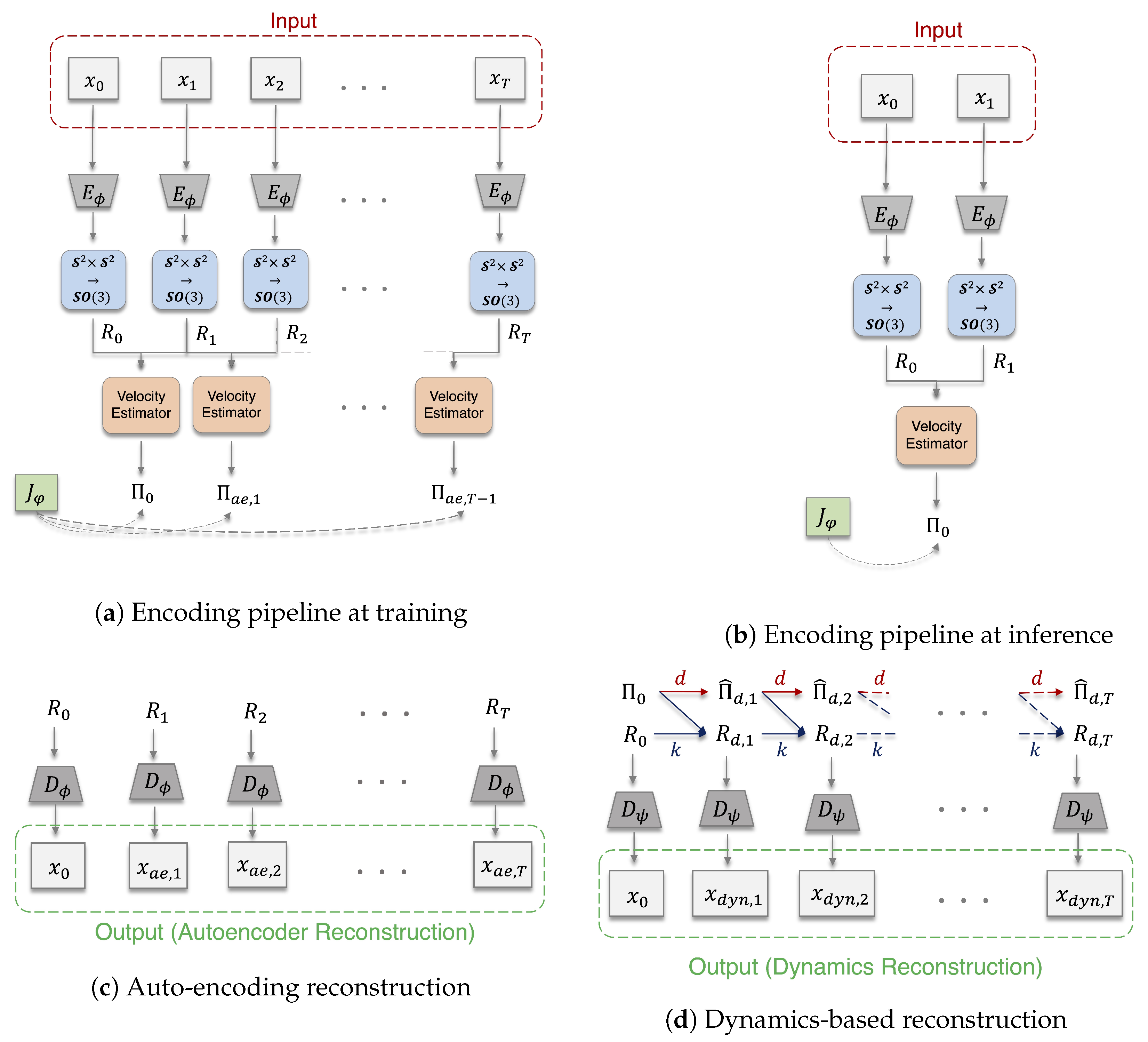
4.2. Embedding Images to an SO(3) Latent Space

In the first stage of our prediction pipeline, we embed image observations of a freely rotating rigid body to a low-dimensional latent representation to facilitate computation of the dynamics. The latent representation is constrained to have the same SO ( 3 ) structure as the configuration space of the rigid body, making learned representations interpretable and compatible with the equations of motion. Our embedding network Φ is given by the composition of functions Φ : = f π E ϕ : I SO ( 3 ) . The convolutional encoding neural network E ϕ : I R 6 parameterized by ϕ maps image observations from image space I to a vector z R 6 . The projection operator π : R 6 S 2 × S 2 decomposes the vector z into the vectors u , v R 3 and normalizes them, i.e.,  π ( z ) = ( u / u , v / v ) . Finally, the function f : S 2 × S 2 SO ( 3 ) maps the normalized vectors u and v to the configuration space using the surjective and differentiable S 2 × S 2 parameterization of SO ( 3 ) (see Section 3.1).

4.3. Computing Dynamics in the Latent Space

In the second stage of our prediction pipeline, we compute the dynamics of the freely rotating rigid body using a Hamiltonian with a learned moment-of-inertia tensor, J φ . The moment-of-inertia tensor, J φ , is parameterized by the vectors φ 1 , φ 2 R 3 , representing the diagonal and off-diagonal components of the matrix, and computed using the Cholesky decomposition [25].
To compute the dynamics, we first construct an initial condition ( R 0 k , Π 0 k ) T * SO ( 3 ) . Given the sequential pair ( R 0 k , R 1 k ) = ( Φ ( x 0 k ) , Φ ( x 1 k ) ) , we perform this in two steps. First, we compute the angular velocity Ω 0 k by Algorithm 1. Then, we compute the angular momentum by the matrix product of the learned moment-of-inertia and angular velocity, i.e.,  Π 0 k = J φ Ω 0 k . With the initial condition ( R 0 k , Π 0 k ) , subsequent angular momenta { Π ^ i k } i = 1 T are computed using the Lie–Poisson Equation (4) and the reduced Hamiltonian formed using the learned momentum-of-inertia J φ . We integrate the Lie–Poisson equations forward in time using a Runge–Kutta fourth-order (RK45) numerical solver [26].
Subsequent rotations { R ^ i k } i = 1 T are computed in two steps. First, we compute the sequence of quaternions { q ^ i k } i = 1 T by Equation (1), using the quaternion representation q 0 k of the initial rotation R 0 k and the initial angular velocity Ω 0 k . We integrate Equation (1) forward in time using an RK45 solver with a normalization step [18] that ensures elements of the resulting sequence are valid quaternions. Then, we transform the sequence of quaternions { q ^ i k } i = 1 T to a sequence of rotations rotations { R ^ i k } i = 1 T using a modified Shepperd’s algorithm [27].
Algorithm 1: An algorithm to calculate the body angular velocity given two sequential orientation matrices and the time step in between them.
Aerospace 10 00921 i001

4.4. Decoding SO(3) Latent States to Images

In the final stage of our prediction pipeline, we decode the sequence of SO ( 3 ) latent states produced by the dynamics pipeline to a sequence of images (see Figure 2d). Our decoding network Ψ is given as the composition of functions Ψ :   = D ψ π 1 f 1 : SO ( 3 ) I , where the convolutional decoding network D ψ : R 6 I parameterized by ψ maps a vector z = ( u , v ) , where ( u , v ) S 2 × S 2 , to the image space I .

4.5. Training Methodology

In this section, we describe the loss functions used to optimize our model: the auto-encoding reconstruction loss ( L ae ), the dynamics-based reconstruction loss ( L dyn ), the latent orientation loss ( L latent , R ), and latent momentum loss ( L latent , Π ). L ae ensures the embedding to SO ( 3 ) is sufficiently expressive to represent the entire image dataset, and L dyn ensures correspondence between the input image sequences and the images sequences produced by the learned dynamics. The latent loss functions, L latent , R and L latent , Π , ensure consistency between the latent states produced by the encoding pipeline and those produced by the dynamics pipeline.
For notational convenience, we denote the encoding pipeline E : I S 3 and the decoding pipeline D : S 3 I . Quantities computed in the encoding pipeline use subscript ae (e.g., R ae k i ), while those computed in the dynamics pipeline use subscript dyn (e.g., R dyn k i ).

4.5.1. Reconstruction Losses

The auto-encoding reconstruction loss is the mean squared error (MSE) between the ground-truth image sequence and the reconstructed image sequence without dynamics:
L ae = 1 N T k = 1 N i = 0 T 1 x i k ( D E ) x i k 2 2 .
The dynamics-based reconstruction loss is the MSE between the ground-truth image sequence and the image sequence produced by the dynamics pipeline:
L dyn = 1 N T k = 1 N i = 1 T x i k D q dyn k i 2 2 .

4.5.2. Latent Losses

We define L latent R as the SO ( 3 ) distance [19] between the 3 × 3 identity matrix and right-difference of orientations produced in the encoding pipeline and the orientations produced in the dynamics pipeline:
L latent R = 1 N T k = 1 N i = 1 T I 3 R ae k i T R dyn k i F 2 .
We define L latent Π as the MSE between the angular momenta estimated in the encoding pipeline and the angular momenta computed in the dynamics pipeline (see Figure 2):
L latent Π = 1 N T k = 1 N i = 1 T Π ae k i Π dyn k i 2 2 .
The hyperparameters we use to train our model are given in Table A2 in Appendix A.3. We train our model for 500 epochs, on a single NVIDIA A100 SXM4 GPU. Our training time is approximately 12 h, and our inference time is approximately 300 milliseconds.

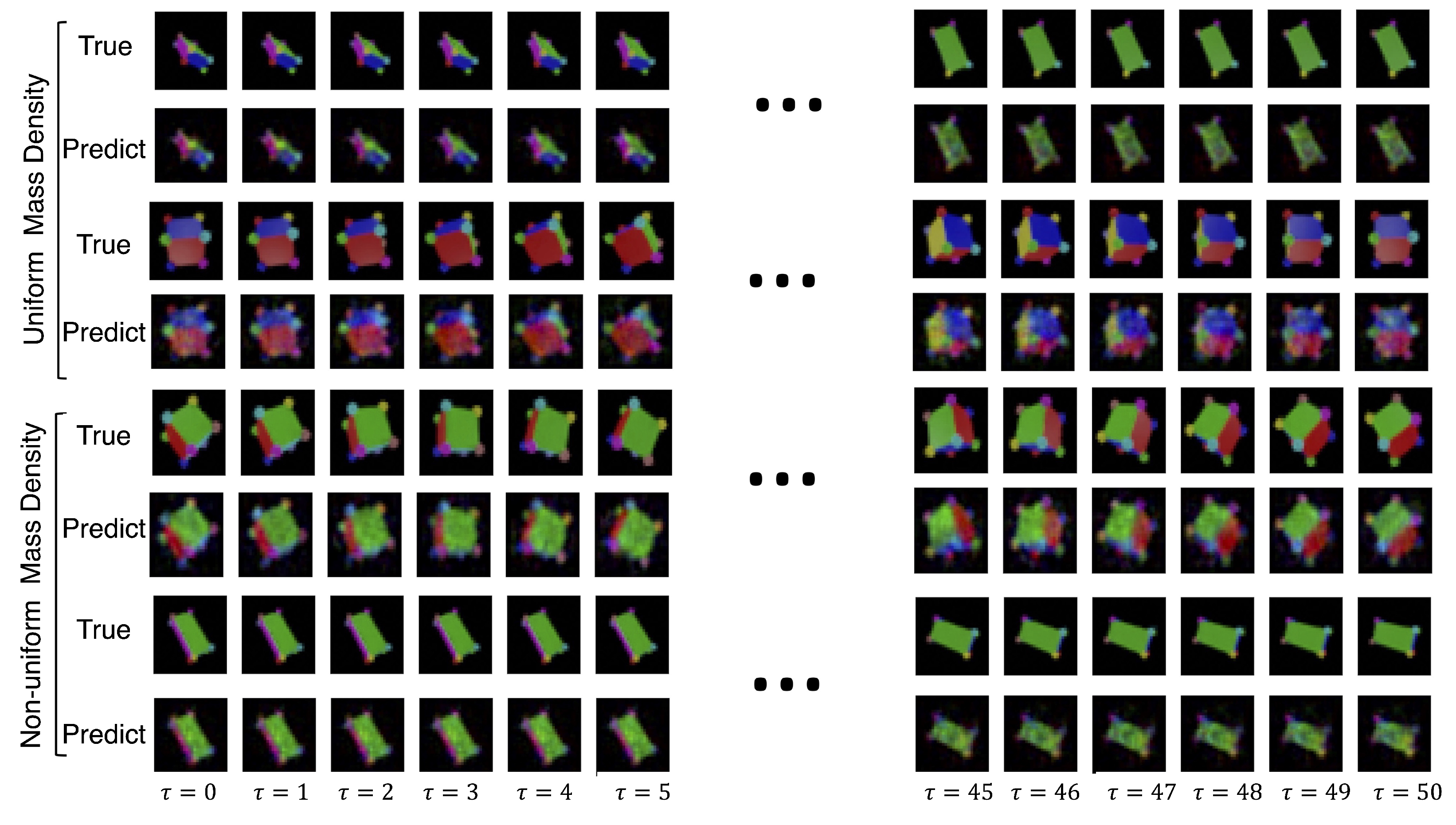
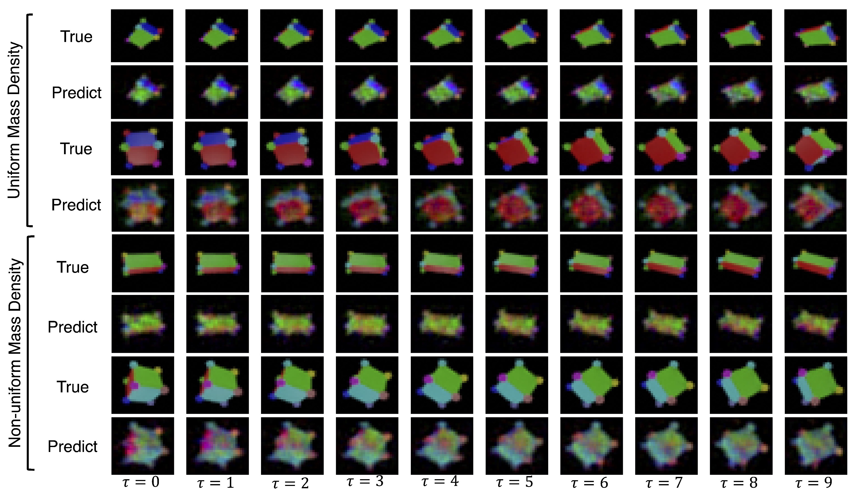
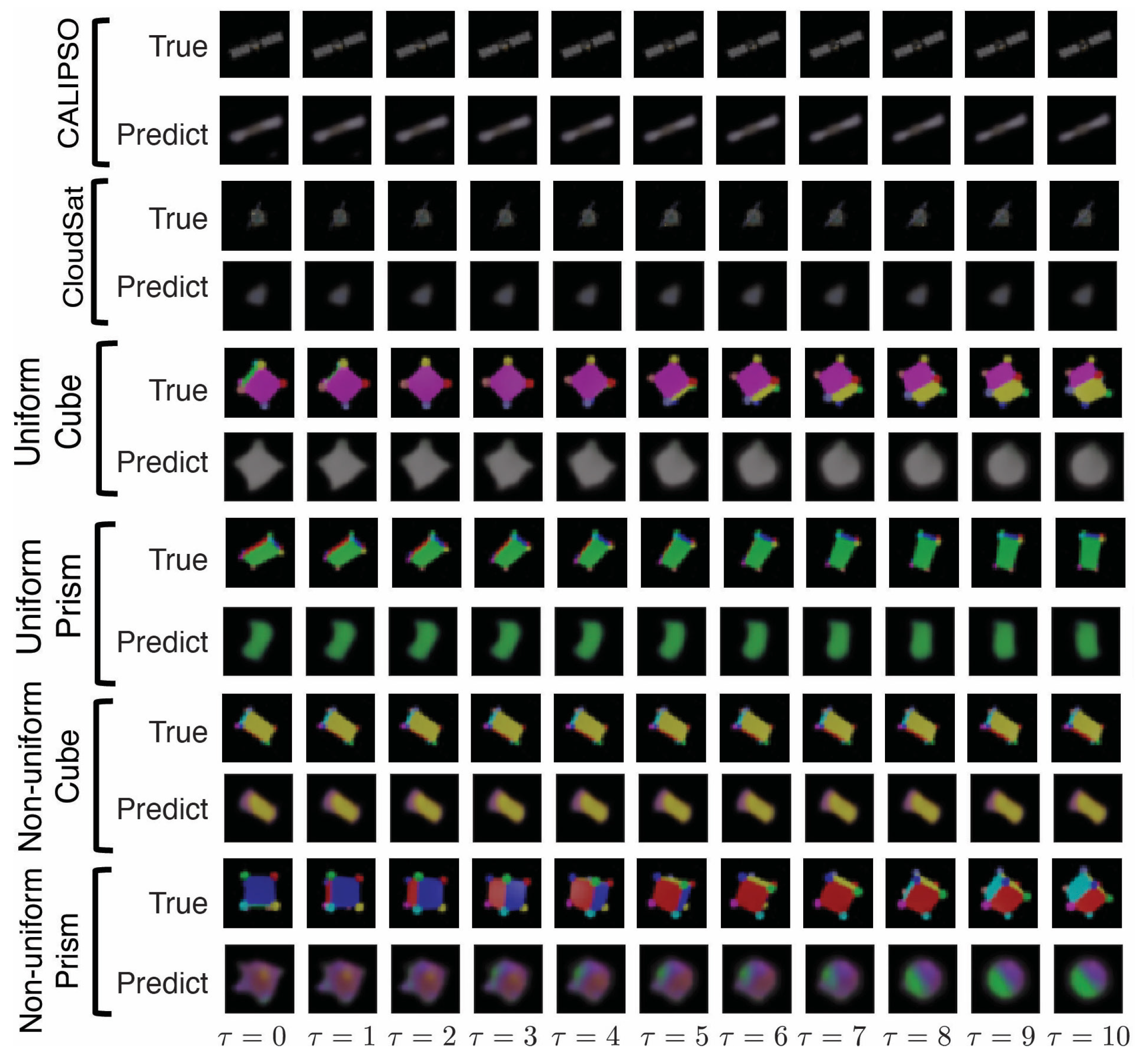
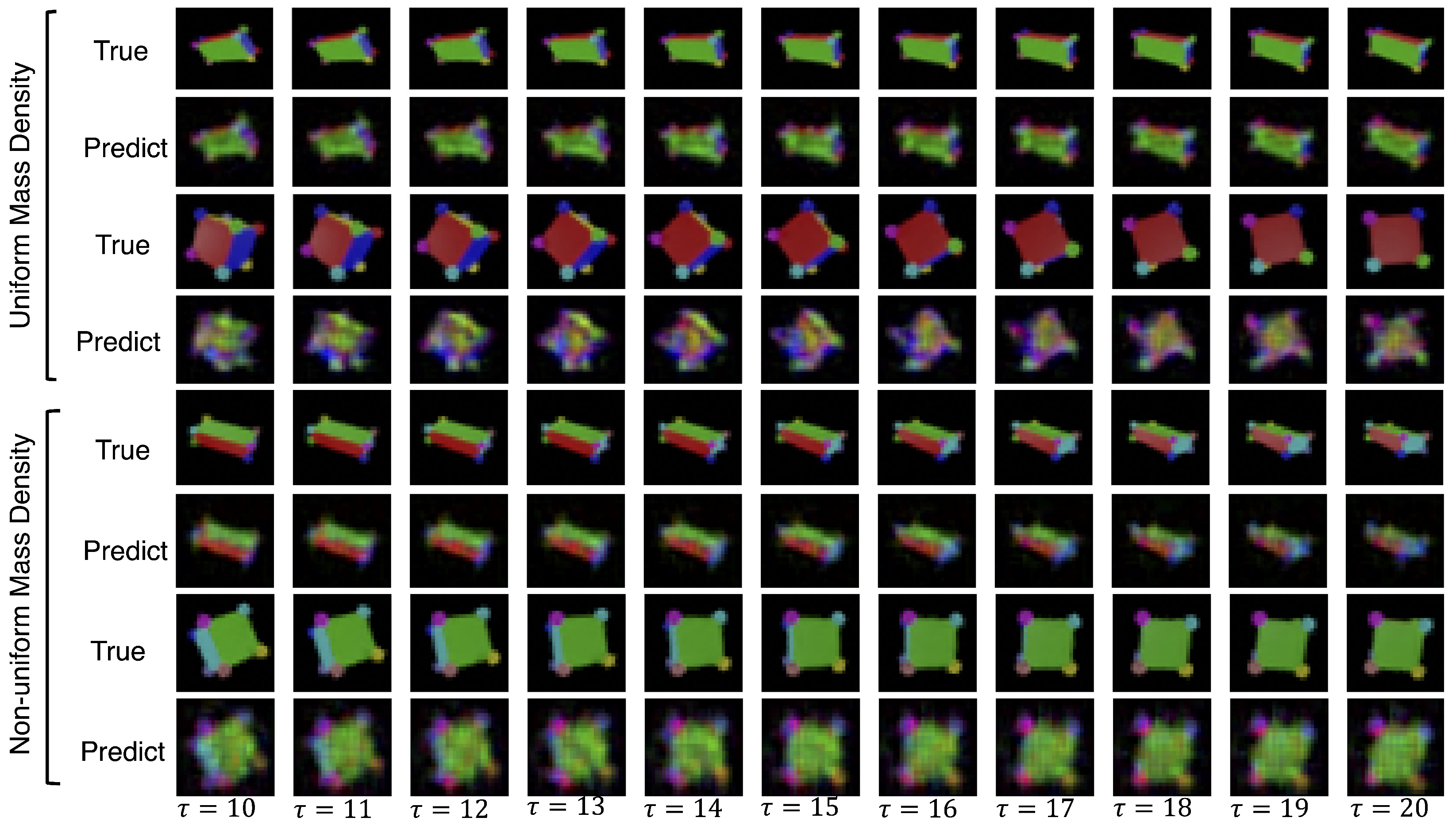
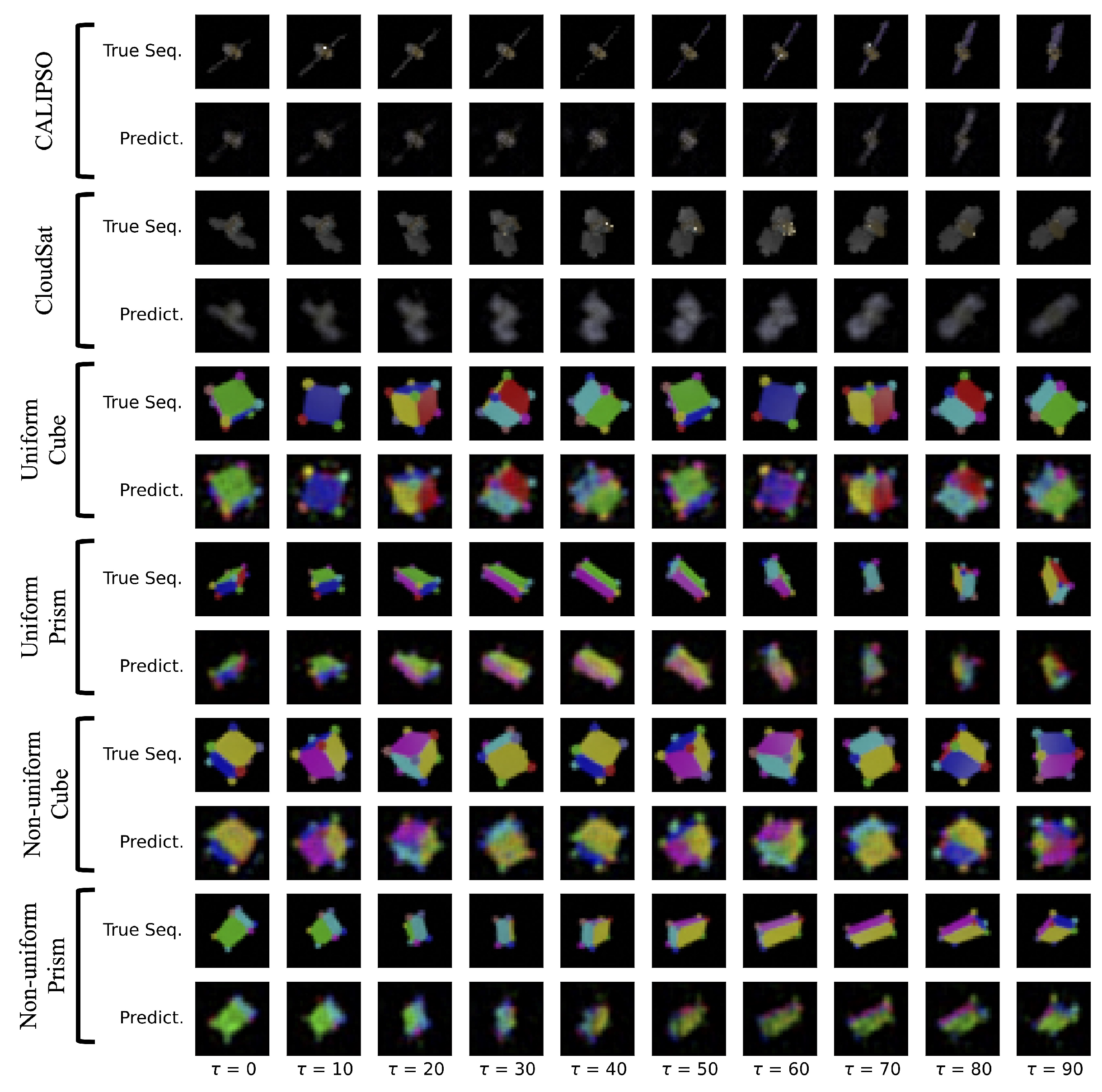
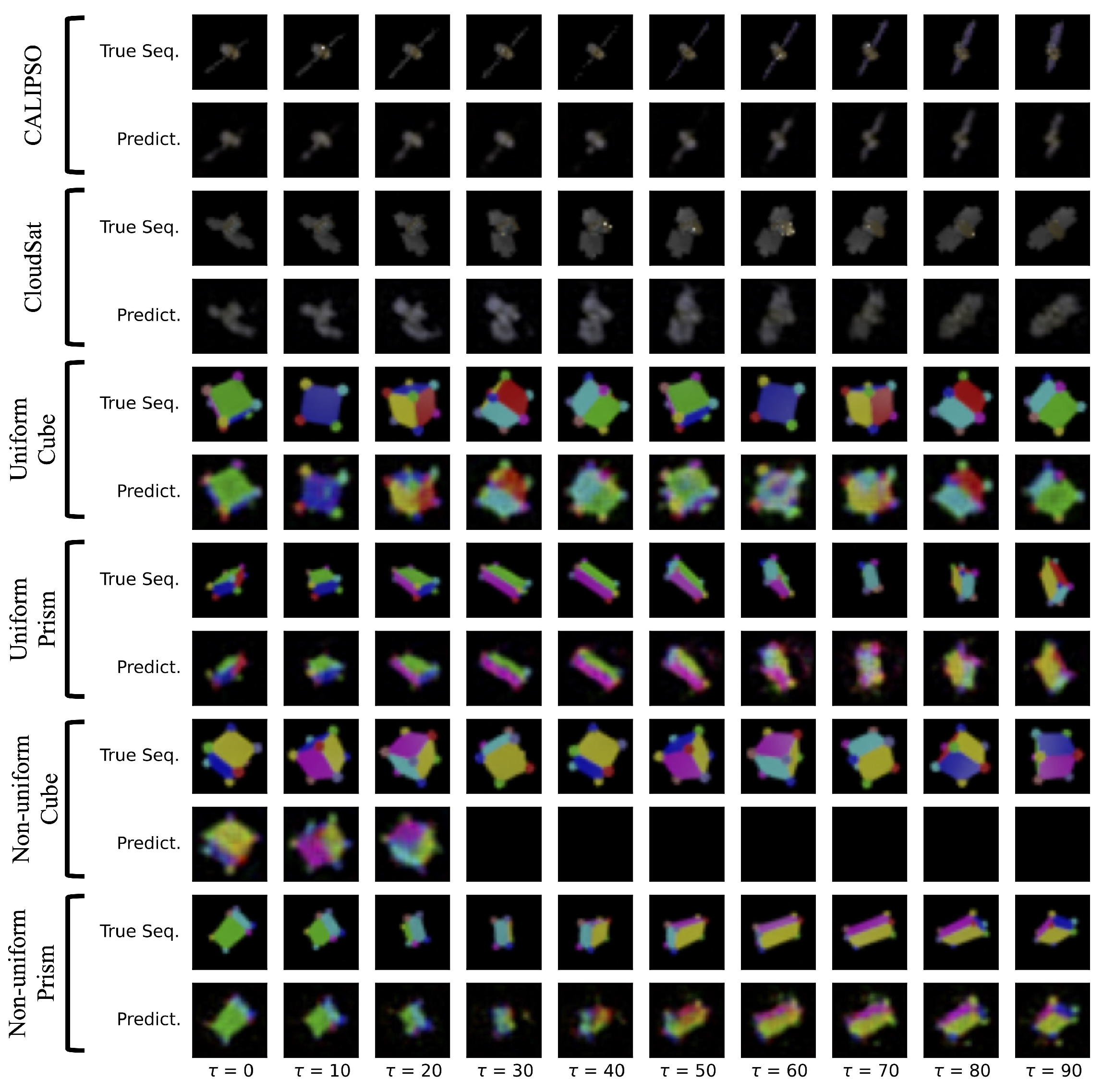
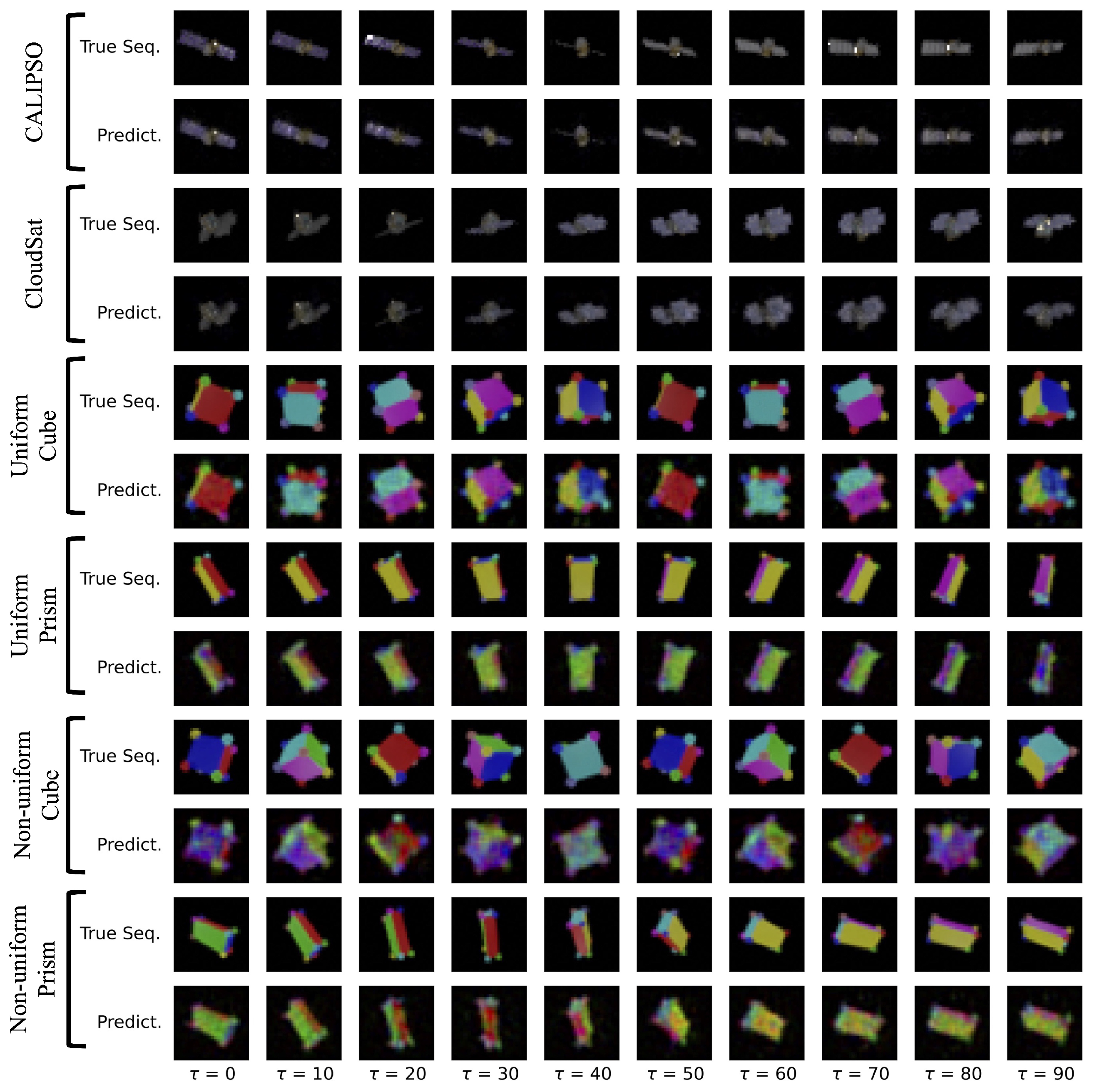
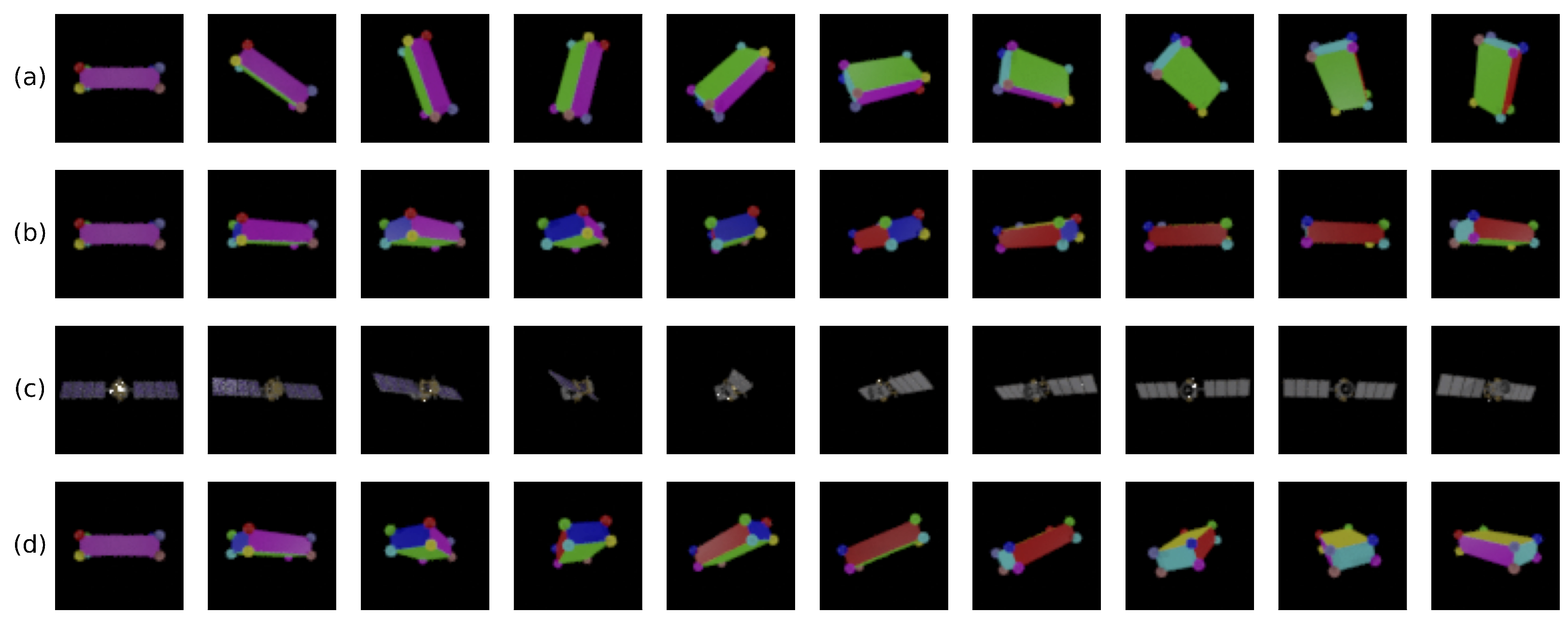
4.6. 3D Rotating Rigid-Body Datasets

To evaluate our model, we introduce six synthetic datasets of freely rotating objects. Previous efforts in learning dynamics from images [4,5,6,10] consider only 2D planar systems (e.g., the simple pendulum, Acrobot, and cart-pole); existing datasets of freely rotating rigid bodies in 3D such as SPEED [28,29], SPEED+ [30], and URSO [31], contain random image-pose pairs rather than sequential pairs needed for video prediction and dynamics extraction. Our datasets showcase the rich dynamical behaviors of 3D rotational dynamics through images, and can be used for 3D dynamics learning tasks. Specifically, we introduce the following five datasets (see Table A1 in Appendix A.2 for moment-of-inertia matrices):
  • Uniform mass density cube: a multi-colored cube of uniform mass density;
  • Uniform mass density prism: a multi-colored rectangular prism with uniform mass density;
  • Non-uniform mass density cube: a multi-colored cube with non-uniform mass density;
  • Non-uniform mass density prism: a multi-colored prism with non-uniform mass density;
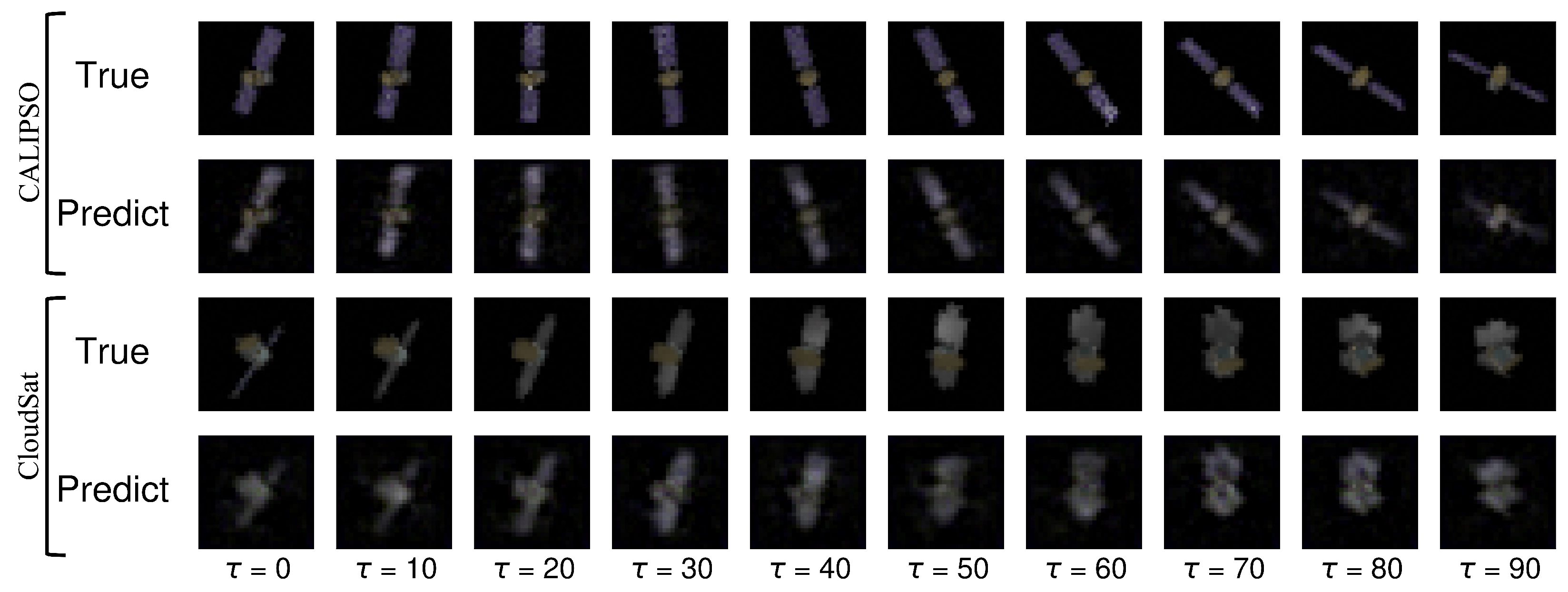
  • Uniform density synthetic-satellites: renderings of CALIPSO and CloudSat satellites with uniform mass density.
For each dataset, N = 1000 trajectories are created. Each trajectory consists of an initial condition x 0 = ( R 0 , Π 0 ) that is integrated forward in time using a Python-based Runge–Kutta solver for T = 100 time steps with spacing Δ t = 10 3 . Initial conditions are chosen such that ( R 0 , Π 0 ) Uniform SO ( 3 ) × S 2 with Π 0 scaled to have Π 0 2 = 50 . The orientations q ^ from the integrated trajectories are passed to Blender [32] to render images of 28 × 28 pixels (as shown in Figure 1).
The synthetic image datasets are generated using Blender [32] with ideal and fixed lighting conditions. Models trained on this dataset may exhibit sensitivity to variations in lighting conditions, and may not generalize to real data.

5. Results

Figure 3 and Figure 4 show the model’s performance on the datasets for both short- and long-term predictions. Figure 3 results show that the model is capable of predicting into the future at least five fold longer than the length of the time horizon used at training time. Figure 4 results show that the model is capable of predicting the future with images of more complex geometries and surface properties, i.e., those of the CALIPSO and CloudSat satellites, at least ten fold longer than the length of the time horizon used at training time. The model’s performance on the datasets is indicative of its capabilities to predict dynamics and map them to image space.
The uniform mass density cube and prism datasets are used to demonstrate baseline capabilities of our approach for image prediction. The non-uniform mass density datasets validate the model’s capability to predict a mass distribution that may not be visible from the exterior, e.g., for an asteroid or space debris or as part of failure diagnostics on a satellite where there may be broken or shifted internal components. The satellite datasets are used to validate the model’s capability to handle bodies with less regular and more realistic external geometries.
We compare the performance of our model to three baseline models: (1) the Long Short Term Memory (LSTM) network, (2) the Neural ODE [33] network, and (3) the Hamiltonian Generative Network (HGN) [5]. Recurrent neural networks like the LSTM-baseline provide a discrete dynamics model. Neural ODE can be combined with a multi-layer perceptron to predict continuous dynamics. HGN is a generative model with a Hamiltonian inductive bias. Architecture and training details for each baseline are given in Appendix A.4. The prediction performances of our model and the baselines are shown in Table 1. Our model has the lowest MSE on the majority of our datasets with good prediction performance on all of our datasets. Our model outperforms the state-of-the-art HGN model, reducing the expected MSE by nearly half on all datasets. Overall, our model outperforms the baseline models on the majority of the datasets with a more interpretable latent space, continuous dynamics, and fewer model parameters.
In Appendix A.5, we present the results of ablations studies and provide discussion. We find that the latent losses improve performance. However, the model may be over constrained with both the dynamics-based and auto-encoding based reconstruction losses.

6. Summary and Conclusions

6.1. Summary

In this work, we have presented the first physics-informed deep learning framework for predicting image sequences of 3D rotating rigid-bodies by embedding the images as measurements in the configuration space SO ( 3 ) and propagating the Hamiltonian dynamics forward in time. We have evaluated our approach on new datasets of free-rotating 3D bodies with different inertial properties, and have demonstrated the ability to perform long-term image predictions. We outperform the LSTM, Neural ODE and Hamiltonian Generative Network (HGN) baselines on our datasets, producing better qualitative predictions and reducing the error observed for the state-of-the-art HGN by a factor of 2.

6.2. Conclusions

By enforcing the representation of the latent space to be SO ( 3 ) , this work provides the advantage of interpretability over black-box physics-informed approaches. The extra interpretability of our approach is a step towards placing additional trust into sophisticated deep learning models. This work provides a natural path to investigating how to incorporate and evaluate the effect of classical model-based control directly to trajectories in the latent space.

7. Future Work

Although our approach so far has been limited to embedding RGB-images of rotating rigid-bodies with configuration spaces in SO ( 3 ) , there are natural extensions to a wider variety of problems. For instance, this framework can be extended to embed different high-dimensional sensor measurements, such as point clouds, by modifying the feature extraction layers of the autoencoder. The latent space can be chosen to reflect generic rigid bodies in SE ( 3 ) or systems in more complicated spaces, such as the n-jointed robotic arm on a restricted subspace of Π i = 1 n SO ( 3 ) . Another possible extension includes multibody systems, i.e., systems with rigid and flexible body dynamics, which would have applications to systems such as spacecraft with flexible solar panels and aircraft with flexible wings.

Author Contributions

J.J.M. and C.A.-B. are the lead authors of this manuscript. Both assisted in conceptualization, methodology, investigation, writing, and editing of the manuscript. J.J.M. also contributed analyses and led software development associated with the model and assisted in software development for data generation. C.A.-B. also contributed compute resources and assisted in software development, and served in a supervisory role. N.Z. contributed to methodology, investigation, and writing and editing of the manuscript, and led data curation and software development for data generation. E.D. provided resources, served in a supervisory role, and assisted in writing and editing of the manuscript. N.E.L. was the principal investigator, contributed to conceptualization, methodology, investigation, writing, and editing the manuscript, and served in a supervisory role and acquired funding. All authors have read and agreed to the published version of the manuscript.

Funding

This research was funded in part by the Office of Naval Research grant number #N00014-18-1-2873 and in part by funding provided by The Aerospace Corporation. The APC was funded by The Aerospace Corporation.

Data Availability Statement

The code used to create and train our model is available https://github.com/CAB-Lab-Princeton/Learning-RBD-from-Images (accessed on 11 September 2023). The dataset generation code is available https://github.com/jjmason687/rbnn_data_generation (accessed on 11 September 2023).

Acknowledgments

Justice Mason and Christine Allen-Blanchette would like to thank Yaofeng Desmond Zhong and Juncal Arbelaiz for their helpful discussions.

Conflicts of Interest

The authors declare no conflict of interest.

Appendix A

Appendix A.1. Rigid Body Rotational Dynamics and Stability

Let J R 3 × 3 denote the moment-of-inertia matrix for a 3D rigid body. The matrix J depends on how mass is distributed inside the body and can be understood to play a role in rotational dynamics that is analogous to, but more complicated than, the role played in translational dynamics of the scalar total body mass m.
Define an orthonormal reference frame B = { i , j , k } fixed to the body with origin at the body’s center of mass. Let r = ( x , y , z ) be a point on the body expressed with respect to B . The distribution of mass inside the rigid body is encoded by density ρ ( r ) , i.e., mass per unit volume of the body at the point r . Let V be the total volume of the body and denote by ⊗ the outer product. J is computed [19] with respect to body frame B as
J = V ρ ( r ) ( r 2 I 3 r r ) d x d y d z .
J is a symmetric positive definite matrix, which means that it can always be diagonalized. If the frame B is chosen so that J is diagonal, the axes of B are called the principal axes and the three diagonal elements of J are called the principal moments of inertia.
Consider, for example, the rectangular prism of Figure 1a,b, which has uniformly distributed mass, i.e., ρ ( r ) = ρ 0 for every point r in the body. Let B be chosen with its first, second, and third axes aligned with the long, intermediate, and short axes of the prism, respectively. Then, the axes of B are the principal axes, J = J 1 is diagonal, and the first, second, and third principal moments of inertia (the diagonal elements of J 1 ) are ordered from smallest to largest. For the very same rectangular prism but with the non-uniform distribution of mass used in Figure 1d, the moment-of-inertia matrix J 3 , with respect to the same frame B , is no longer diagonal and its principal moments of inertia are different from those in the uniform case. J 1 and J 3 as well other moment-of-inertia matrices used for experiments in this work are given in Appendix A.2.
Let Ω 0 = Ω ( 0 ) be the initial body angular velocity. Euler’s equations [19] describe the rotational dynamics of the body, i.e., the evolution over time t of Π given J and Ω 0 :
d Π ( t ) d t = Π ( t ) × J 1 Π ( t ) , Π ( 0 ) = J Ω 0 ,
where × is the vector cross product. The corresponding evolution of body angular velocity over time is Ω ( t ) = J 1 Π ( t ) , where Π ( t ) is the solution of (A2).
Given Ω ( t ) , t 0 , the evolution of orientation over time is computed from the rigid body kinematics equations:
d R ( t ) d t = R ( t ) Ω × ( t ) ,
where Ω × is the 3 × 3 skew-symmetric matrix defined by ( Ω × ) y = Ω × y for y R 3 .
For the rotational dynamics (A2), there are three equilibrium solutions, i.e., where d Π ( t ) / d t = 0 , corresponding to steady spin about the short principal axis, intermediate principal axis, and long principal axis, respectively. Steady spin about the short axis and long axis is stable, which means that an initial angular velocity near either of these solutions yields a spinning behavior, independent of exterior geometry (see Figure 1b,c). Steady spin about the intermediate axis is unstable, which means that an initial angular velocity near this solution yields a tumbling behavior (see Figure 1a).
Figure 1a,b shows that for the same prism with the same (uniform) mass distribution, and thus the same moment-of-inertia matrix J 1 , different values of initial body angular velocity result in very different behavior: an unstable tumble in Figure 1a and a stable spin in Figure 1b. Figure 1b,d shows that for the same prism with the same initial angular velocity, different mass distributions yield different behaviors, a steady spin in (b) when J = J 1 and a wobble in (d) when J = J 3 . Figure 1b,c shows that the rotational dynamics of a rigid body with the same moment-of-inertia matrix J 1 and same initial body angular velocity yield the same behavior, despite different exterior geometries, i.e., the prism in (b) and the CALIPSO satellite in (d).
These cases illustrate that without a way of inferring the underlying mass distribution and estimating initial conditions, there is no way to predict the dynamics from images.

Appendix A.2. Dataset Generation Parameters

Appendix A.2.1. Uniform Mass Density Cube

The moment-of-inertia tensor and its inverse for the uniform mass density cube are given by the matrices J 0 and J 0 1 in Table A1. The principal axes of rotation expressed in the body-fixed reference frame are also given in Table A1, showing the principal axes and body-fixed reference frame are aligned.
Table A1. Table containing the moment-of-inertia tensors, inverse moment-of-inertia tensors, and principal axes used to generate training data for each object.
ObjectMoment-of-Inertia TensorInverse Moment-of-Inertia TensorPrincipal Axes
Uniform Cube J 0 = 1 3 1 0 0 0 1 0 0 0 1 J 0 1 = 3 0 0 0 3 0 0 0 3 1 0 0 , 0 1 0 , 0 0 1
Uniform Prism J 1 = 0.42 0 0 . 0 1.41 0 0 0 1.67 J 1 1 = 2.40 0 0 0 0.71 0 0 0 0.60 1 0 0 , 0 1 0 , 0 0 1
Non-uniform Cube J 2 = 0.17 0 0.56 0 0.17 0.99 0.56 0.99 0.17 J 2 1 = 4.53 2.62 0.44 2.62 1.34 0.78 0.44 0.78 0.13 0.35 0.62 0.71 , 0.87 0.49 0 , 0.35 0.62 0.71
Non-uniform Prism J 3 = 0.47 0 0.28 0 1.61 0.49 0.28 0.49 1.83 J 3 1 = 2.37 0.12 0.39 0.12 0.68 0.20 0.39 0.20 0.66 0.35 0.62 0.71 , 0.87 0.49 0 , 0.35 0.62 0.71
CALIPSO J 4 = 0.33 0 0 0 0.50 0 0 0 1.0 J 4 1 = 3.0 0 0 0 2.0 0 0 0 1.0 1 0 0 , 0 1 0 , 0 0 1
CloudSat J 5 = 0.33 0 0 0 0.50 0 0 0 1.0 J 5 1 = 3.0 0 0 0 2.0 0 0 0 1.0 1 0 0 , 0 1 0 , 0 0 1

Appendix A.2.2. Uniform Mass Density Prism

The moment-of-inertia tensor and its inverse for the uniform mass density prism are given by the matrices J 1 and J 1 1 in Table A1. The principal axes of rotation expressed in the body-fixed reference frame are also given in Table A1, showing the principal axes and body-fixed reference frame are aligned.

Appendix A.2.3. Non-Uniform Mass Density Cube

The moment-of-inertia tensor and its inverse for the non-uniform mass density cube are given by the matrices J 2 and J 2 1 in Table A1. The principal axes of rotation expressed in the body-fixed reference frame are also given in Table A1, and are not aligned with body-fixed reference frame.

Appendix A.2.4. Non-Uniform Mass Density Prism

The moment-of-inertia tensor and its inverse for the non-uniform mass density prism are given by the matrices J 3 and J 3 1 in Table A1. The principal axes of rotation expressed in the body-fixed reference frame are also given in Table A1, and are not aligned with body-fixed reference frame.

Appendix A.2.5. CALIPSO

The moment-of-inertia tensor and its inverse for the CALIPSO satellite are given by the matrices J 4 and J 4 1 in Table A1. The principal axes of rotation expressed in the body-fixed reference frame are also given in Table A1, i.e., the principal axes and body-fixed reference frame are aligned.

Appendix A.2.6. CloudSat

The moment-of-inertia tensor and its inverse for the CloudSat satellite are given by the matrices J 5 and J 5 1 in Table A1. The principal axes of rotation expressed in the body-fixed reference frame are also given in Table A1, i.e., the principal axes and body-fixed reference frame are aligned.

Appendix A.3. Hyperparameters

The hyperparameters used to train our model are given in Table A2. Hyperparameters, distinct from model parameters, control the training process. We optimize over the model parameters using the Adam optimizer [35].
Table A2. Hyperparameters used to train model for the non-uniform mass density prism experiment. Only values differing from default values are given in the table.
Experiment Hyperparameters
Parameter Name Value
Random seed0
Test dataset split0.2
Validation dataset split0.1
Number of epochs1000
Batch size256
Autoencoder learning rate 1 × 10 3
Dynamics learning rate 1 × 10 3
Sequence length10
Time step 1 × 10 3

Appendix A.4. Performance of Baseline Models

We compare the performance of our model against three baseline architectures: (1) LSTM, (2) Neural ODE [33], and (3) Hamiltonian Generative Network (HGN) [5]. LSTM and Neural ODE baselines are trained using the same autoencoder architecture as our model, while HGN is trained with the autoencoder architecture described in Toth et al. [5]. The LSTM- and Neural ODE-baseline differ from our approach in how the dynamics are computed, emphasizing the beneficial role of Hamiltonian structure as well as our SO ( 3 ) latent space.

Appendix A.4.1. LSTM-Baseline

The LSTM-baseline uses an LSTM network to predict dynamics in the latent space. The LSTM-baseline is a three-layer LSTM network with an input dimension of 6 and a hidden dimension of 50. The hidden state and cell state are randomly initialized and the output of the network is mapped to a six-dimensional latent vector by a linear layer. The LSTM-baseline predicts a single step forward using the nine previous states as input. We train the LSTM by minimizing the sum of the auto-encoding and dynamics-based reconstruction losses, L ae and L dyn as defined in Section 4.5. At inference, we use a recursive strategy to predict farther into the future using previously predicted states to predict subsequent states. The qualitative performance of the LSTM-baseline is given in Figure A1, and the quantitative performance is given in Table 1. The total number of parameters in the network is 52,400. The LSTM-baseline has poorer performance than our proposed approach on all evaluated datasets.
Figure A1. Predicted sequences for uniform/non-uniform prism and cube datasets given by the LSTM-baseline. The figure shows time steps τ = 10 through τ = 20 . These are the first 11 predictions of the model.
Aerospace 10 00921 g0a1

Appendix A.4.2. Neural ODE [33]-Baseline

The Neural ODE-baseline uses the Neural ODE [33] framework to predict dynamics in the latent space. The Neural ODE-baseline is a three-layer multilayer perceptron (MLP) that uses the ELU [36] nonlinear activation function. The baseline has an input dimension of 6, a hidden dimension of 50, and an output dimension of 6. The Neural ODE-baseline predicts a sequence of latent states using a single initial latent state. We train the Neural ODE-baseline by minimizing the sum of the auto-encoding and dynamics-based reconstruction losses, L ae and L dyn , as defined in Section 4.5. We use the RK4-integrator to integrate the learned dynamics. The qualitative performance for the Neural ODE-baseline is given in Figure A2, and the quantitative performance is given in Table 1. The total number of parameters in the network is 11,406. The Neural ODE-baseline has poorer performance than our proposed approach on all evaluated datasets.
Figure A2. Predicted sequences for uniform/non-uniform prism and cube datasets given by the Neural ODE-baseline.
Aerospace 10 00921 g0a2

Appendix A.4.3. Hamiltonian Generative Network (HGN)

HGN [5] uses a combination of a variational auto-encoding (VAE) neural network and Hamiltonian dynamics to perform video prediction. When testing HGN as a baseline, we use the implementation provided by Balsells Rodas et al. [37]. We train HGN on our datasets using the hyperparameters, loss function, and integrator described in Toth et al. [5]. The qualitative performance for the HGN-baseline is given in Figure A3, and the quantitative performance is given in Table 1.

Appendix A.5. Ablation Studies

In our ablation studies, we explore the impact of the reconstruction losses and latent losses on the performance of our model (see Section 4.5.1 and Section 4.5.2 for the definition of our losses). The ablated models are trained similarly to the proposed model, but parts of the loss functions are removed. In the first ablation study, only the dynamics-based reconstruction loss ( L dyn ) is used, i.e., the auto-encoding reconstruction loss ( L ae ) and latent losses ( L latent R and L latent Π ) are removed from the total loss function. In the second ablation study, only the auto-encoding reconstruction and dynamics-based reconstruction losses ( L ae and L dyn ) are used, i.e., the latent losses ( L latent R and L latent Π ) are removed from the total loss function. In the final ablation study, only the dynamics-based reconstruction and latent losses are used ( L dyn , L latent R , and L latent Π ), i.e., the auto-encoding reconstruction loss ( L ae ) is removed from the total loss function. These ablation studies demonstrate the prediction performance of the model when trained with (1) the dynamics-based reconstruction loss only, (2) the auto-encoding reconstruction and dynamics-based reconstruction losses, and (3) the dynamics-based reconstruction loss and latent losses. In the first two cases of the ablation study, the prediction performance worsens on the majority of the datasets, but in the third case, the prediction performance improves over the proposed model on the majority of the datasets. It may be that model is over constrained with both the dynamics-based and auto-encoding based reconstruction losses. From Table A3 and Figure A4, it can be inferred that only using the dynamics-based reconstruction loss negatively affects the prediction performance of our proposed model (although it is still better than the baselines in Table 1).
Figure A3. Predicted sequences for all datasets given by the Hamiltonian Generative Network (HGN) baseline. The figure shows timesteps τ = 0 through τ = 10 .
Aerospace 10 00921 g0a3
Figure A4. Evaluation of the image prediction performance of an ablated version of our model trained with only the dynamics-based reconstruction loss ( L dyn ) from Section 4.5.1. The ablated model has poorer performance than the proposed approach over all datasets. The prediction performance worsens earlier than the proposed model’s performance, as shown in Figure 3.
Aerospace 10 00921 g0a4
Table A3 and Figure A5 and Figure A6 also demonstrate the positive impact of the latent losses on prediction performance for our model. We see worsened average pixel MSE and prediction with the latent losses removed. These results are further corroborated in the literature [6,38]. Furthermore, Figure A6 show a better prediction performance when the auto-encoding reconstruction loss is removed. This could indicate that the L ae loss is over-constraining the proposed model.
Table A3. Average pixel MSE over a 30-step unroll on the train and test data on four datasets for our ablation study.
Dataset L total L dyn L dyn + L ae L dyn + L latent
TRAIN TEST TRAIN TEST TRAIN TEST TRAIN TEST
Uniform Prism3.03 ± 1.263.05 ± 1.213.99 ± 1.213.74 ± 0.933.99 ± 1.503.85 ± 1.454.82 ± 1.325.09 ± 1.53
Uniform Cube4.13 ± 2.144.62 ± 2.025.73 ± 0.515.87 ± 0.567.11 ± 2.636.95 ± 2.412.80 ± 0.182.80 ± 0.20
Non-uniform Prism4.98 ± 1.267.07 ± 1.884.27 ± 1.283.89 ± 1.103.86 ± 1.383.66 ± 1.274.16 ± 1.275.09 ± 1.53
Non-uniform Cube7.27 ± 1.065.65 ± 1.506.23 ± 0.885.93 ± 0.85--8.78 ± 0.938.64 ± 1.14
CALIPSO1.18 ± 0.431.19 ± 0.632.00 ± 0.781.85 ± 0.581.73 ± 0.731.62 ± 0.500.49 ± 0.070.54 ± 0.18
CloudSat1.32 ± 0.741.56 ± 1.010.96 ± 0.171.39 ± 0.480.87 ± 0.291.40 ± 0.400.28 ± 0.060.28 ± 0.06
Figure A5. Evaluation of the image prediction performance of an ablated version of our model trained with only the auto-encoding reconstruction and dynamics-based reconstruction losses ( L ae and L dyn ) from Section 4.5.1. The ablated model has poorer performance than the proposed approach over all datasets—even failing to predict after ∼30 time steps for the non-uniform cube dataset.
Aerospace 10 00921 g0a5
Figure A6. Evaluation of the image prediction performance of an ablated version of our model trained with only dynamics-based reconstruction losses and latent losses ( L dyn , L latent R , and L latent Π ) from Section 4.5.1. The ablated model has better performance than the proposed approach on the majority of the datasets– implying that the proposed model may be over constrained.
Aerospace 10 00921 g0a6

References

  1. Williams, B.; Antreasian, P.; Carranza, E.; Jackman, C.; Leonard, J.; Nelson, D.; Page, B.; Stanbridge, D.; Wibben, D.; Williams, K.; et al. OSIRIS-REx Flight Dynamics and Navigation Design. Space Sci. Rev. 2018, 214, 69. [Google Scholar] [CrossRef]
  2. Flores-Abad, A.; Ma, O.; Pham, K.; Ulrich, S. A review of space robotics technologies for on-orbit servicing. Prog. Aerosp. Sci. 2014, 68, 1–26. [Google Scholar] [CrossRef]
  3. Mark, C.P.; Kamath, S. Review of active space debris removal methods. Space Policy 2019, 47, 194–206. [Google Scholar] [CrossRef]
  4. Zhong, Y.D.; Leonard, N.E. Unsupervised Learning of Lagrangian Dynamics from Images for Prediction and Control. In Proceedings of the Conference on Neural Information Processing Systems 2020, Virtual, 6–12 December 2020. [Google Scholar]
  5. Toth, P.; Rezende, D.J.; Jaegle, A.; Racanière, S.; Botev, A.; Higgins, I. Hamiltonian Generative Networks. In Proceedings of the International Conference on Learning Representations 2020, Addis Ababa, Ethiopia, 26–30 April 2020. [Google Scholar]
  6. Allen-Blanchette, C.; Veer, S.; Majumdar, A.; Leonard, N.E. LagNetViP: A Lagrangian Neural Network for Video Prediction. arXiv 2020, arXiv:2010.12932. [Google Scholar]
  7. Byravan, A.; Fox, D. SE3-nets: Learning Rigid Body Motion Using Deep Neural Networks. In Proceedings of the International Conference on Robotics and Automation 2017, Singapore, 29 May–3 June 2017. [Google Scholar]
  8. Peretroukhin, V.; Giamou, M.; Rosen, D.M.; Greene, W.N.; Roy, N.; Kelly, J. A Smooth Representation of Belief over SO(3) for Deep Rotation Learning with Uncertainty. arXiv 2020, arXiv:2006.01031. [Google Scholar]
  9. Duong, T.; Atanasov, N. Hamiltonian-based Neural ODE Networks on the SE(3) Manifold For Dynamics Learning and Control. In Proceedings of the Robotics: Science and Systems, Virtual, 12–16 July 2021. [Google Scholar]
  10. Greydanus, S.; Dzamba, M.; Yosinski, J. Hamiltonian Neural Networks. In Proceedings of the Conference on Neural Information Processing Systems, Vancouver, BC, Canada, 8–14 December 2019. [Google Scholar]
  11. Chen, Z.; Zhang, J.; Arjovsky, M.; Bottou, L. Symplectic Recurrent Neural Networks. In Proceedings of the International Conference on Learning Representations 2020, Addis Ababa, Ethiopia, 26–30 April 2020. [Google Scholar]
  12. Cranmer, M.; Greydanus, S.; Hoyer, S.; Battaglia, P.W.; Spergel, D.N.; Ho, S. Lagrangian Neural Networks. In Proceedings of the International Conference on Learning Representations 2020, Addis Ababa, Ethiopia, 26–30 April 2020. [Google Scholar]
  13. Kingma, D.P.; Welling, M. Auto-Encoding Variational Bayes. arXiv 2014, arXiv:1312.6114. [Google Scholar]
  14. Falorsi, L.; de Haan, P.; Davidson, T.R.; Cao, N.D.; Weiler, M.; Forré, P.; Cohen, T.S. Explorations in Homeomorphic Variational Auto-Encoding. In Proceedings of the International Conference of Machine Learning Workshop on Theoretical Foundations and Application of Deep Generative Models, Stockholm, Sweden, 14–15 July 2018. [Google Scholar]
  15. Levinson, J.; Esteves, C.; Chen, K.; Snavely, N.; Kanazawa, A.; Rostamizadeh, A.; Makadia, A. An analysis of svd for deep rotation estimation. Adv. Neural Inf. Process. Syst. 2020, 33, 22554–22565. [Google Scholar]
  16. Brégier, R. Deep regression on manifolds: A 3D rotation case study. In Proceedings of the 2021 International Conference on 3D Vision (3DV), London, UK, 1–3 December 2021; pp. 166–174. [Google Scholar]
  17. Zhou, Y.; Barnes, C.; Lu, J.; Yang, J.; Li, H. On the Continuity of Rotation Representations in Neural Networks. In Proceedings of the 2019 IEEE/CVF Conference on Computer Vision and Pattern Recognition (CVPR), Long Beach, CA, USA, 15–20 June 2019; pp. 5738–5746. [Google Scholar]
  18. Andrle, M.S.; Crassidis, J.L. Geometric Integration of Quaternions. AIAA J. Guid. Control 2013, 36, 1762–1772. [Google Scholar] [CrossRef]
  19. Goldstein, H.; Poole, C.P.; Safko, J.L. Classical Mechanics; Addison Wesley: Boston, MA, USA, 2002. [Google Scholar]
  20. Zhong, Y.D.; Dey, B.; Chakraborty, A. Symplectic ODE-Net: Learning Hamiltonian Dynamics with Control. In Proceedings of the International Conference on Learning Representations 2020, Addis Ababa, Ethiopia, 26–30 April 2020. [Google Scholar]
  21. Zhong, Y.D.; Dey, B.; Chakraborty, A. Dissipative SymODEN: Encoding Hamiltonian Dynamics with Dissipation and Control into Deep Learning. In Proceedings of the ICLR 2020 Workshop on Integration of Deep Neural Models and Differential Equations, Addis Ababa, Ethiopia, 26–30 April 2020. [Google Scholar]
  22. Finzi, M.; Wang, K.A.; Wilson, A.G. Simplifying Hamiltonian and Lagrangian Neural Networks via Explicit Constraints. Conf. Neural Inf. Process. Syst. 2020, 33, 13. [Google Scholar]
  23. Lee, T.; Leok, M.; McClamroch, N.H. Global Formulations of Lagrangian and Hamiltonian Dynamics on Manifolds; Springer: Cham, Switzerland, 2018. [Google Scholar]
  24. Marsden, J.E.; Ratiu, T.S. Introduction to Mechanics and Symmetry; Texts in Applied Mathematics; Springer: New York, NY, USA, 1999. [Google Scholar]
  25. Lin, Z. Riemannian Geometry of Symmetric Positive Definite Matrices via Cholesky Decomposition. SIAM J. Matrix Anal. Appl. 2019, 40, 1353–1370. [Google Scholar] [CrossRef]
  26. Atkinson, K.A. An Introduction to Numerical Analysis; John Wiley & Sons: Hoboken, NJ, USA, 1989. [Google Scholar]
  27. Markley, F.L. Unit quaternion from rotation matrix. AIAA J. Guid. Control 2008, 31, 440–442. [Google Scholar] [CrossRef]
  28. Kisantal, M.; Sharma, S.; Park, T.H.; Izzo, D.; Martens, M.; D’Amico, S. Satellite Pose Estimation Challenge: Dataset, Competition Design, and Results. IEEE Trans. Aerosp. Electron. Syst. 2020, 56, 4083–4098. [Google Scholar] [CrossRef]
  29. Sharma, S.; Beierle, C.; D’Amico, S. Pose estimation for non-cooperative spacecraft rendezvous using convolutional neural networks. In Proceedings of the 2018 IEEE Aerospace Conference, Big Sky, MT, USA, 3–10 March 2018; pp. 1–12. [Google Scholar] [CrossRef]
  30. Park, T.H.; Märtens, M.; Lecuyer, G.; Izzo, D.; D’Amico, S. SPEED+: Next-Generation Dataset for Spacecraft Pose Estimation across Domain Gap. In Proceedings of the 2022 IEEE Aerospace Conference (AERO), Big Sky, MT, USA, 5–12 March 2022; pp. 1–15. [Google Scholar] [CrossRef]
  31. Proença, P.F.; Gao, Y. Deep Learning for Spacecraft Pose Estimation from Photorealistic Rendering. In Proceedings of the 2020 IEEE International Conference on Robotics and Automation (ICRA), Paris, France, 31 May–31 August 2020; pp. 6007–6013. [Google Scholar] [CrossRef]
  32. Community, B.O. Blender—A 3D Modelling and Rendering Package; Blender Foundation, Stichting Blender Foundation: Amsterdam, The Netherlands, 2018. [Google Scholar]
  33. Chen, R.T.; Rubanova, Y.; Bettencourt, J.; Duvenaud, D.K. Neural ordinary differential equations. Adv. Neural Inf. Process. Syst. 2018, 31, 1–13. [Google Scholar]
  34. Hochreiter, S.; Schmidhuber, J. Long short-term memory. Neural Comput. 1997, 9, 1735–1780. [Google Scholar] [CrossRef] [PubMed]
  35. Kingma, D.P.; Ba, J. Adam: A method for stochastic optimization. arXiv 2014, arXiv:1412.6980. [Google Scholar]
  36. Clevert, D.A.; Unterthiner, T.; Hochreiter, S. Fast and accurate deep network learning by exponential linear units (elus). arXiv 2015, arXiv:1511.07289. [Google Scholar]
  37. Balsells Rodas, C.; Canal Anton, O.; Taschin, F. [Re] Hamiltonian Generative Networks. ReScience C 2021, 7. [Google Scholar] [CrossRef]
  38. Watter, M.; Springenberg, J.T.; Boedecker, J.; Riedmiller, M. Embed to control: A locally linear latent dynamics model for control from raw images. Adv. Neural Inf. Process. Syst. 2015, 27, 1–9. [Google Scholar]
Figure 1. Simulations illustrating how mass distribution and initial angular velocity determine behavior. (a) Tumbling prism: uniform mass distribution ( J = J 1 ) and initial angular velocity near an unstable solution. (b) Spinning prism: J = J 1 and initial angular velocity near a stable solution. (c) Spinning CALIPSO satellite: J = J 1 and same initial angular velocity as (b). (d) Wobbling prism: non-uniform mass distribution ( J = J 3 ) and same initial velocity as (b).
Aerospace 10 00921 g001
Figure 2. A schematic of the model’s forward pass at training time and inference.
Aerospace 10 00921 g002
Figure 3. Predicted sequences for uniform and non-uniform mass density cube and prism datasets given by our model. The figure shows predicted images at time steps τ = 0 to 5 and τ = 45 to 50.
Aerospace 10 00921 g003
Figure 4. Predicted sequences for the CALIPSO satellite (top) and CloudSat satellite (bottom) with uniform mass densities given by our model. The figure shows predicted images at every 10th time step from τ = 0 to 90.
Aerospace 10 00921 g004
Table 1. Average pixel mean square error over a 30-step prediction on the train and test data on six datasets. All values are multiplied by 1 × 10 3 . We evaluate our model and compare to three baseline models: (1) recurrent model (LSTM [34]), (2) Neural ODE ([33]), and (3) HGN ([5]).
DatasetOursLSTM-BaselineNeural ODE-BaselineHGN
TRAIN TEST TRAIN TEST TRAIN TEST TRAIN TEST
Uniform Prism2.66 ± 0.102.71 ± 0.083.46 ± 0.593.47 ± 0.613.96 ± 0.684.00 ± 0.684.18 ± 0.07.80 ± 0.30
Uniform Cube3.54 ± 0.173.97 ± 0.1621.55 ± 1.9821.64 ± 2.129.48 ± 1.199.43 ± 1.2017.43 ± 0.0018.69 ± 0.12
Non-uniform Prism4.27 ± 0.186.61 ± 0.884.50 ± 1.314.52 ± 1.344.67 ± 0.584.75 ± 0.596.16 ± 0.088.33 ± 0.26
Non-uniform Cube6.24 ± 0.294.85 ± 0.357.47 ± 0.517.51 ± 0.507.89 ± 1.507.94 ± 1.5914.11 ± 0.1318.14 ± 0.36
CALIPSO0.79 ± 0.530.87 ± 0.500.62 ± 0.210.65 ± 0.220.69 ± 0.260.71 ± 0.271.18 ± 0.021.34 ± 0.05
CloudSat0.64 ± 0.450.65 ± 0.290.89 ± 0.360.93 ± 0.430.65 ± 0.220.66 ± 0.251.48 ± 0.041.66 ± 0.11
Number of Parameters652,40011,400-
Disclaimer/Publisher’s Note: The statements, opinions and data contained in all publications are solely those of the individual author(s) and contributor(s) and not of MDPI and/or the editor(s). MDPI and/or the editor(s) disclaim responsibility for any injury to people or property resulting from any ideas, methods, instructions or products referred to in the content.

