1. Introduction
Over the past few years, the adoption of unmanned aerial vehicles (UAVs) or drones in commercial and civilian applications has increased significantly due to advances in manufacturing processes, resulting in their economic feasibility. This increase in usage has opened up an extensive range of potential applications, including photography, aerial inspection, disaster relief, traffic control, precision agriculture, delivery systems, and communications. Consequently, regulatory bodies and authorities have developed frameworks to ensure the safe and effective use of UAVs. For example, the Federal Aviation Administration (FAA) in the United States has issued operational regulations for small unmanned aircraft systems (UASs) weighing under 25 kg for civilian applications. Additionally, the FAA has launched the “Drone Integration Pilot Program” to facilitate the exploration of expanded UAV applications. This program includes rules for night flights, applications requiring UAVs to fly over people, and beyond visual line of sight (BVLoS) operations [
1].
The issue of communication with cellular-connected UAVs has gained significant attention in recent times [
2]. Existing cellular networks have not been specifically optimised to support UAVs and are primarily focused on providing high-quality service to terrestrial users. Given the stringent regulatory requirements, the need for extensive research and standardization efforts to ensure the reliable operation of UAVs in a range of deployment scenarios is evident. These factors highlight the importance of optimizing current cellular networks to facilitate seamless communication with UAVs.
Novel guidelines and programs like the FAA’s “Drone Integration Pilot Program” are expected to accelerate the growth of the UAV industry globally. Thus, UAVs are seen as an interesting opportunity for businesses in the next decade.
One of the prominent technologies to enable UAV communications is fifth-generation (5G) cellular technology. Indeed, 5G technology will ultimately replace fourth-generation (4G) networks as the new standard cellular networks. Currently, it provides connectivity to most cell phones, and 5G is beneficial because it is expected to provide higher download speeds and greater bandwidth. The future infrastructure of 5G networks can therefore link seamlessly and ubiquitously with everything. For instance, one attractive and growing technology is the Internet of Things (IoT), which has generated a tremendous increase in data traffic, thus leading to the requirement of advanced networks to cope with reliability and traffic requirements.
The realization of 5G and beyond 5G (B5G) wireless networks is crucial to meet the requirements of connected UAVs. These networks offer low latency, high speed, massive capacity, and edge computing, which can enable UAVs to operate virtually in real time. This translates to fewer incidents of loss of control and mid-air collisions, making 5G networks a critical component for the safe and efficient operation of UAVs. Therefore, there is an urgent need to accelerate the development and deployment of 5G networks to support the growth of the UAV industry [
3].
Although 5G networks can provide high data rates and low latency, they may not be fully optimised for UAVs and may face challenges such as signal blockage and limited coverage. Therefore, we may need to consider using sixth-generation (6G) networks, which are expected to provide advanced features such as intelligent networking, enhanced sensing and perception, and autonomous decision making to resolve current challenges in communication with UAVs. However, it should be noted that the scope of our project does not include the development of 6G networks [
4,
5].
The utilization of UAVs in communication confers various promising advantages, including the ability for ad-hoc deployment, adaptable network reconfiguration, and a higher probability of achieving line of sight (LOS) links. UAVs that function as 5G base stations, referred to as Next Generation Node Bs (gNBs), represent one of the most remarkable examples and are anticipated to perform a critical role in forthcoming generations of wireless networks, as stated by [
6]. The benefits provided by UAV-gNBs, like swift deployment, mobility, increased likelihood of unimpeded propagation, and flexibility, have gained extensive interest and are being widely investigated.
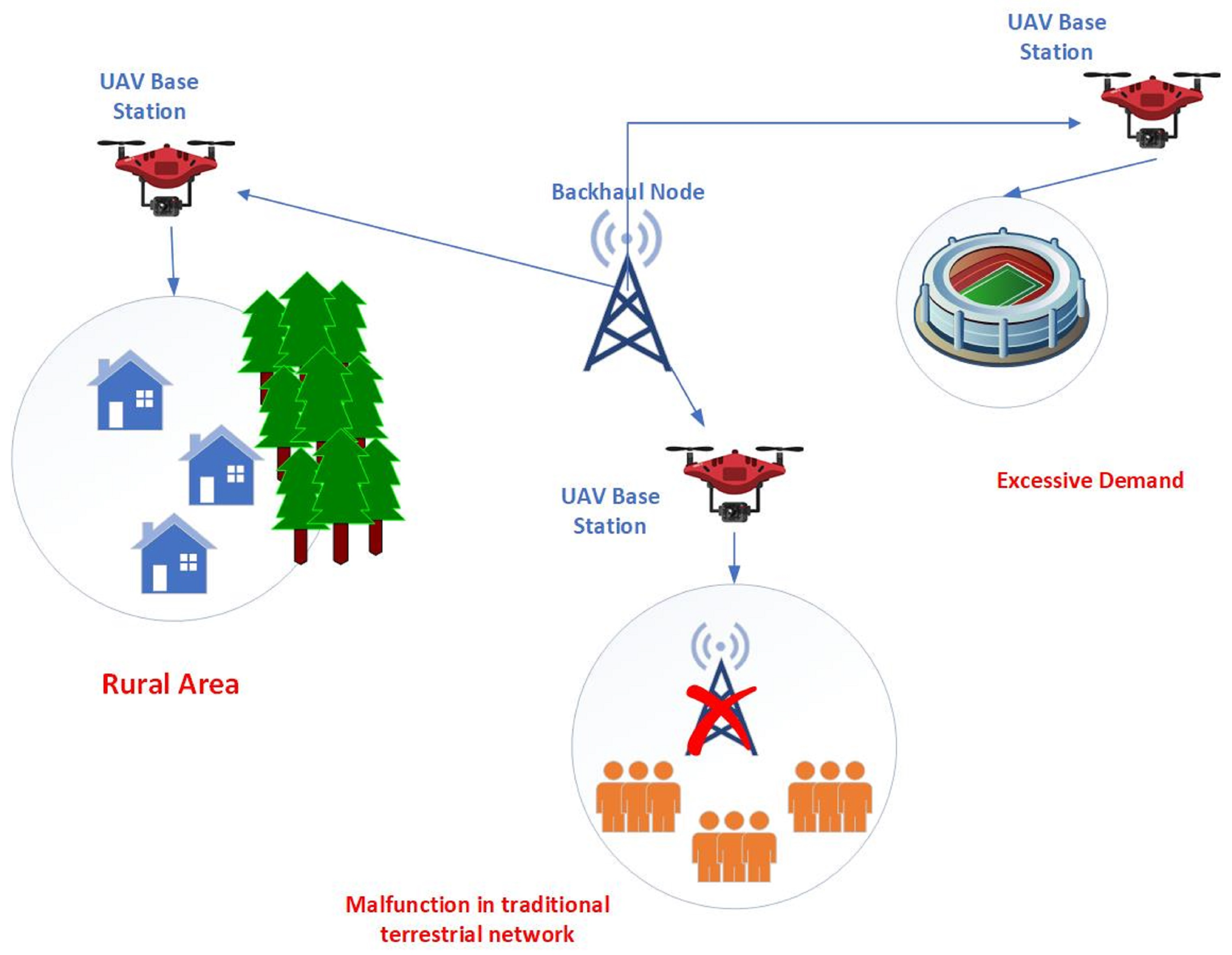
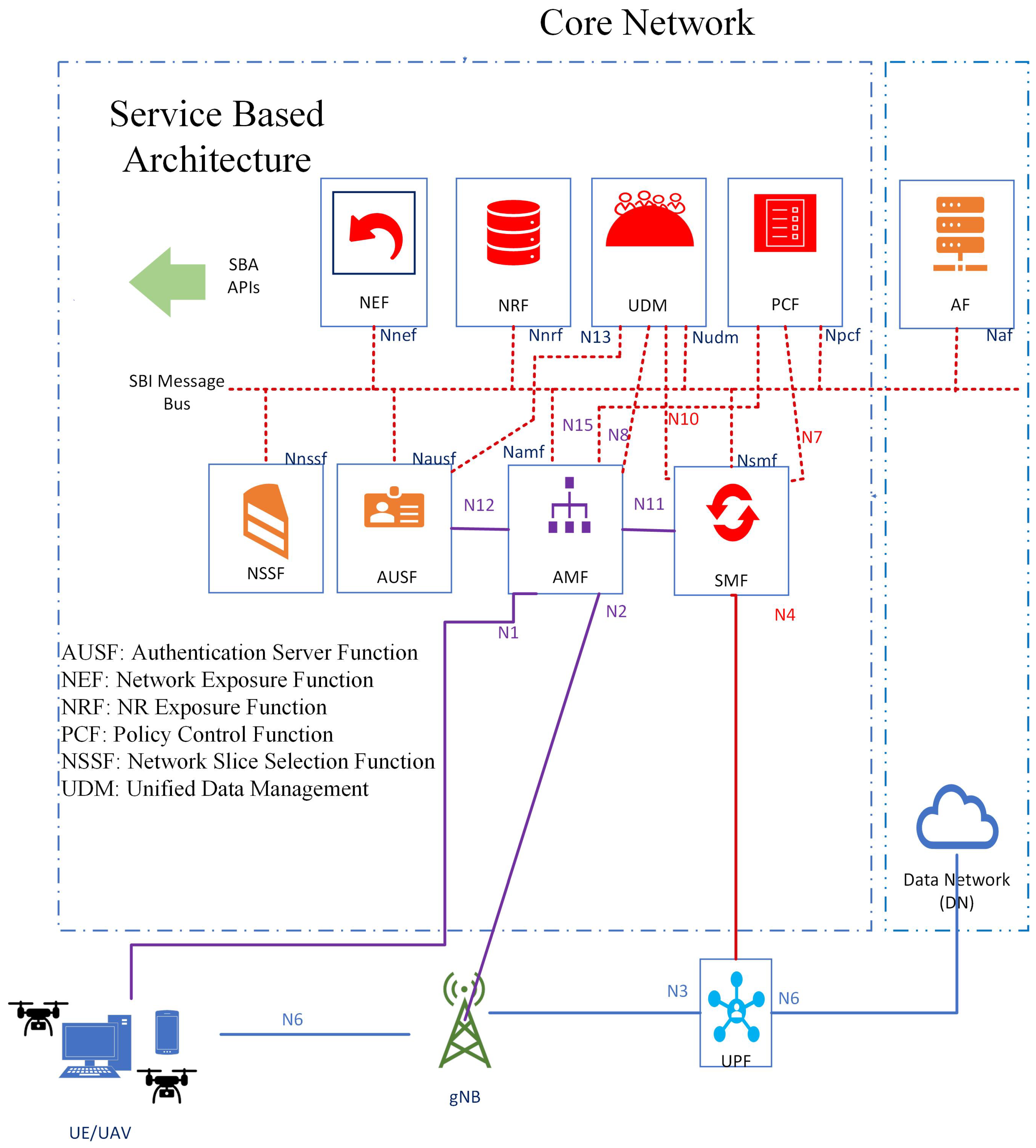
Figure 1 demonstrates several use cases for 5G, including (i) serving as a backup in areas where a gNB malfunction occurs; (ii) providing coverage in rural areas with limited or no gNB infrastructure; and (iii) enhancing quality of service (QoS) in areas with unexpected surges in demand, such as densely populated sports events, by establishing a network connected to the 5G core network via a backhaul node. Further details on the software-based architecture (SBA) of 5G will be presented in the following sections.
At present, communication between UAVs and the ground is restricted to visual line of sight (VLoS) range, which limits reliability, coverage, security, and performance. To overcome these limitations, it is crucial to connect drones to cellular networks to enable BVLoS capabilities. While integrating drones with 5G offers several advantages, it also poses certain challenges [
7,
8,
9,
10,
11].
Contributions
The purpose of this paper is to develop a technique for performing power control to mitigate interference in UAVs operating within 5G networks. To achieve this goal, a novel method of power control is proposed, deviating from conventional approaches. Specifically, this method regulates transmit power not only at the serving gNB but also controls transmit powers of interfering gNBs from a central location. This approach introduces a race condition where the serving gNB for one UAV can act as an interfering gNB for another user. To address this challenge, deep reinforcement learning is employed due to its proven effectiveness in resolving similar problems.
The deep Q-learning (DQL) algorithm is considered a promising solution to the interference problem as it eliminates the need for reporting channel state information (CSI), thereby reducing overhead and resulting in a low-complexity system design. Under the DQL approach, UAVs report only their received signal-to-interference-and-noise ratio (SINR) and coordinates, while the gNB, supported by a cloud-based architecture, performs power control to mitigate interference. This approach involves both associated and interfering gNBs issuing power control commands, diverging from industry standards where only the associated gNB is involved. Building upon our previous work [
12], this paper presents the following significant contributions:
Develops a power control optimization problem for the downlink direction to maximise the SINR experienced by the UAV.
Develops a framework based on deep reinforcement learning (DRL) that enables the concurrent execution of multiple actions and dynamically adjusts power levels to achieve optimal SINR by utilizing data from a given dataset.
Thus, the paper presents a comprehensive framework based on DRL to optimise the SINR experienced by UAVs through dynamic adjustment of power levels using data from a provided dataset. The paper follows a systematic approach, beginning with a literature review and identification of research gaps in
Section 2. This is followed by a discussion of the challenges posed by current interference mitigation techniques in
Section 3.
Section 4 provides a detailed analysis of 5G and UAV technology and their functionalities. In
Section 5, the paper introduces DRL, its components, neural network architecture, and policy selection methods.
Section 6 presents a comparison of existing interference mitigation techniques with the proposed solution and describes the proposed algorithm. The simulation environment, setup, and results obtained are discussed in
Section 7. The paper concludes with a discussion on the impact assessment of the results in
Section 8.
2. Background and Related Works
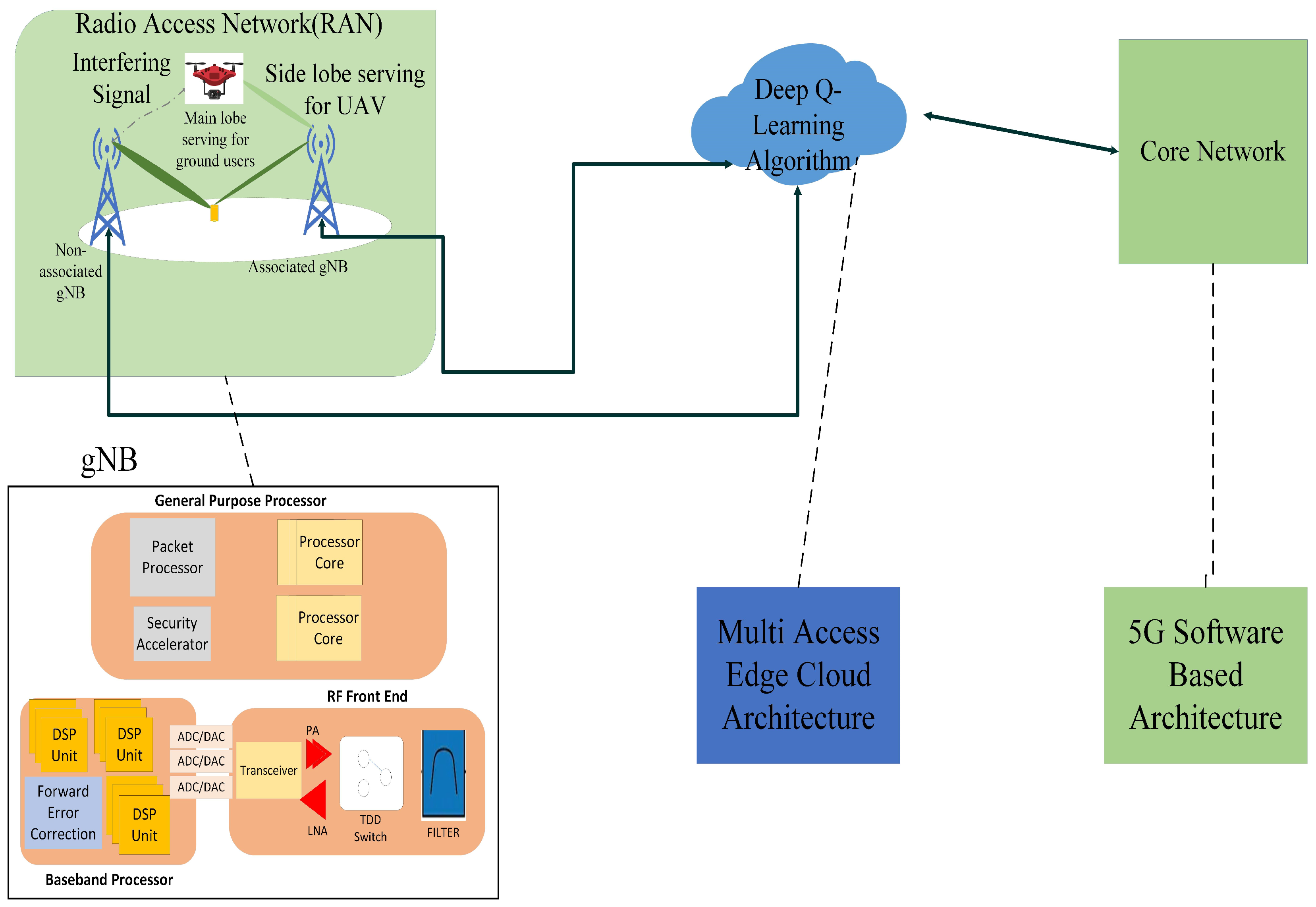
The utilization of UAVs for meeting the growing communication needs has been widely advocated. Despite this, operation of UAVs at high altitude would enable LoS links to be significantly pervasive within the viable communication channels; as a result, a UAV has a high likelihood of communicating with both associated gNBs and interfering gNBs simultaneously. In the case of ground users, who are served by the primary lobe of the gNB antenna, an escalation in pathloss typically correlates with a reduction in interfering signals. However, when UAVs are served by the side lobes of the gNB antenna, the relationship between increasing pathloss and interference becomes less straightforward. This complexity arises because side lobes have the potential to introduce unintended coverage areas and additional propagation paths, thereby giving rise to interference with other systems or gNBs. Consequently, even when the main lobe signal strength is weakened due to pathloss, these side lobes can still generate interference. This scenario increases the likelihood of interference as compared to ground-based users, posing a significant challenge for interference management in cellular networks that include UAVs. Several techniques have been proposed in extant literature to mitigate interference in terrestrial networks, including inter-cell interference coordination (ICIC) [
13,
14] and coordinated multi-point (CoMP) transmission [
15,
16]. However, these techniques prove inadequate in handling new interference challenges arising from UAVs and the emergence of LoS-dominated air–ground links at high altitudes.
ICIC is a radio resource management technique used to enhance spectral efficiency. This is achieved by imposing constraints on the management block to improve favourable channel conditions for a subset of users significantly affected by interference. The coordination of resources may be achieved through fixed, adaptive, or real-time approaches, supported by additional inter-cell signalling, with the frequency adjusted based on specific requirements. A cooperative interference cancellation technique is proposed in [
17] to minimise the sum rate to available gNBs and eliminate co-channel interference at each occupied gNB for multi-beam UAV uplink communication. Although similar techniques have been extensively studied in terrestrial cellular networks [
18], they are not effective in mitigating strong UAV interference, leading to limited frequency reuse in the network and lower spectral efficiency for both UAVs and ground users [
19]. In [
20], the interference in directional UAV networks is characterised using stochastic geometry, considering UAVs equipped with directional antennas and situated in a 3D environment. This work provides a comprehensive analysis of the interference in directional UAV networks, but no strategies are presented for mitigating it.
The approach of employing a path planning or trajectory design to avoid or minimise interference is a widely adopted strategy for interference management. In the paper [
21], the authors consider a relay-assisted UAV network overlaid with an existing network and propose a joint power and 3D trajectory design approach to reposition the UAVs in 3D space to circumvent interference. They propose a joint optimisation solution based on spectral graph theory and convex optimisation to address the problem of 3D trajectory design and power allocation. The simulation results demonstrate that the proposed algorithm improves the maximum flow and reduces undesirable interference to the coexisting network [
22].
The authors of [
23] explore the joint trajectory and power control (TPC) design problem for multi-user UAV-enabled interference channels (UAV-IC). As the TPC problem is NP-hard and involves a significant number of optimisation variables, the authors propose effective sub-optimal algorithms. Although a multi-UAV setup is considered in both [
22] and [
23], the trajectory optimisation approach may not be optimal in situations where the path or trajectory of the UAV is unknown beforehand or changes during the mission.
In [
24], an alternative solution to mitigate UAV–ground interference is proposed by utilizing intelligent reflective surfaces (IRSs) near gNBs for both downlink and uplink communications. The authors suggest an optimal passive beamforming design using IRSs for the downlink to minimise terrestrial interference with UAVs, and a hybrid linear and nonlinear interference coordination (IC) scheme in the uplink to handle the strong interference from UAVs. The authors further investigate the optimal performance of this scheme. However, it should be noted that IRSs are unsuitable for digital applications as they are designed based on the concept of analog beamforming. In [
25], an interference-aware energy-efficient scheme is proposed to allow cellular-connected aerial users to reduce the interference they impose on terrestrial users while maximizing their energy efficiency and spectral efficiency. The optimization problem is formulated considering the key performance indicator (KPI) requirements for both aerial and terrestrial users, including energy efficiency, spectral efficiency, and interference. The problem is solved through the use of a deep Q-learning approach. However, it is critical to note the energy efficiency problem cannot be universally solved as it is dependent on various factors, such as mission design, UAV capabilities, and UAV size.
In recent years, artificial intelligence (AI) has emerged as a critical technology for 5G-and-beyond wireless networks that include UAVs, as demonstrated in studies like [
26]. This is primarily due to AI’s capacity to handle complex problems and large amounts of data in system design and optimisation, making it a crucial tool for creating highly dynamic UAV communication networks. Conventional offline and model-driven trajectory design methods are limited in practical scenarios with variable traffic and open operating environments due to the requirement for accurate communication models and complete understanding of system parameters. However, with the use of deep reinforcement learning, UAVs can predict future network states in real time and adjust communication resource allocation and UAV trajectories accordingly. Additionally, AI-embedded UAVs can play a significant role in edge computing applications, where multiple UAVs can collaborate as aerial edge servers or edge devices for efficient data and computation offloading.
Several research studies have investigated the application of DRL in the field of communications in recent years, as evidenced by publications such as [
8,
27,
28,
29]. In particular, ref. [
29] employs DRL for power regulation in millimeter-wave (mm-wave) transmission as an alternative to beamforming for enhancing non-line-of-sight (NLoS) performance. The authors employ DRL to tackle the power allocation problem with the objective of maximizing the aggregate rate of the user equipment (UE) while meeting quality and transmission power constraints. The proposed approach involves estimating the Q-function of the DRL problem using a convolutional neural network. In another work, ref. [
30] introduces a policy framework that employs DQL to maximise the number of transmissions in a multi-channel access network. In [
31], the authors propose a joint optimization approach that employs a Q-learning algorithm to optimise power control, interference coordination, and communication performance for end-users in a 5G wireless network, enhancing the downlink SINR in a multi-access Orthogonal Frequency Division Multiplexing (OFDM) network from a gNB with multiple antennas to UEs with a single antenna. Finally, ref. [
32] uses DQL to develop a policy to maximise transmissions in a dynamic correlated multi-channel access scenario. It is important to note, however, that these studies only address interference in the context of mobile devices. Neural networks were used in [
28] to forecast mm-wave beams with low training overhead utilising received signals from nearby gNBs. Ref. [
31] analysed voice signals for a multiple-access network consisting of many gNBs. The mid-band 5G frequency was only discussed in the [
33] framework in a single gNB scenario. Deep neural networks, which need channel knowledge to make decisions, were used in [
33] to perform joint beamforming and interference cooperation at mm-wave. The effectiveness of deep neural networks for beamforming without using reinforcement learning was examined in [
34]. These works have deployed machine learning algorithms to implement beamforming to solve the interference problem. Although beamforming improves the SINR of the system and resists interference, it is very complicated and expensive in terms of the hardware to be deployed. Advanced techniques such as double deep Q-learning were discussed in [
35]. The main difference between DQL and double deep Q-learning (DDQL) is that DDQL uses two separate deep neural networks to estimate the Q-values, whereas DQL uses only one. The idea behind DDQL is to reduce the overestimation of Q-values that can occur in DQL. However, in some cases, such as when dealing with interference in 5G networks, overestimation may not be a problem and may even be desirable. In the case of interference in 5G networks, the goal is to minimise the interference between different channels and users. This can be achieved by optimizing the transmission power and frequency allocation of different users. In this scenario, DQL may be more suitable than DDQL because it allows for more exploration of the state–action space, which can lead to better performance in complex environments. Additionally, DQL has been shown to be more computationally efficient than DDQL, which can be a critical factor when dealing with large-scale 5G networks with many users and channels.
The literature review is summarised in
Table 1 and the outcomes are discussed in the following section.
Outcome
UAVs are frequently touted as a promising solution for a wide range of applications, and, as such, the future 5G networks are expected to be able to support UAVs flying at higher altitudes and speeds with minimal interference.
Within the existing literature, many works discuss interference mitigation techniques; however, they also have certain drawbacks and unsuitability to the problem at hand. Methods such as ICIC, as discussed in [
17,
18,
19,
20], are effective for reducing interference via coordination; however, in dynamic and unpredictable environments, such as UAVs in 5G networks, they would be ineffective. In addition, they also generate high overhead, thus increasing the complexity. Another method employed within the literature is path planning for UAVs, as discussed in [
21,
22]. This optimises the trajectory of the UAV so it can take the path with the least interference possible. One clear disadvantage of this would relate to not knowing the path of the UAV beforehand. In addition, dynamic routes could also render this method ineffective. Even though current AI/ML approaches such as [
8,
27,
28,
29,
30] have been effective at mitigating interference, these methods have been deployed for UAVs in general or for users in 5G networks but not both, which is the unique problem that the proposed method in this paper solves. In
Table 1, the literature is summarised and shows that the current solutions for mitigating interference are not sufficient. To address this issue, this paper proposes an interference mitigation approach building upon the work presented in [
12].
3. Interference Mitigation Challenges
When comparing UAVs to traditional ground UEs, it is important to note that UAVs typically operate at higher altitudes. This presents a unique challenge for gNBs as they must provide 3D communication coverage instead of the usual 2D coverage for ground UEs. While conventional gNBs are angled downward to serve ground users and minimise inter-cell interference, UAVs must be integrated into this 3D communication network. This introduces new challenges that must be addressed in order to achieve effective and seamless communications. One of the most critical challenges in UAV communication within a cellular network is interference management. Interference in aerial users is exacerbated by LoS-dominated UAV-gNB channels, which is largely due to the high altitude of UAVs. As a result, this phenomenon represents a significant obstacle to the proper functioning of UAVs in the network. In summary, the integration of UAVs into cellular networks requires careful consideration of 3D coverage, interference management, and other challenges unique to aerial communication.
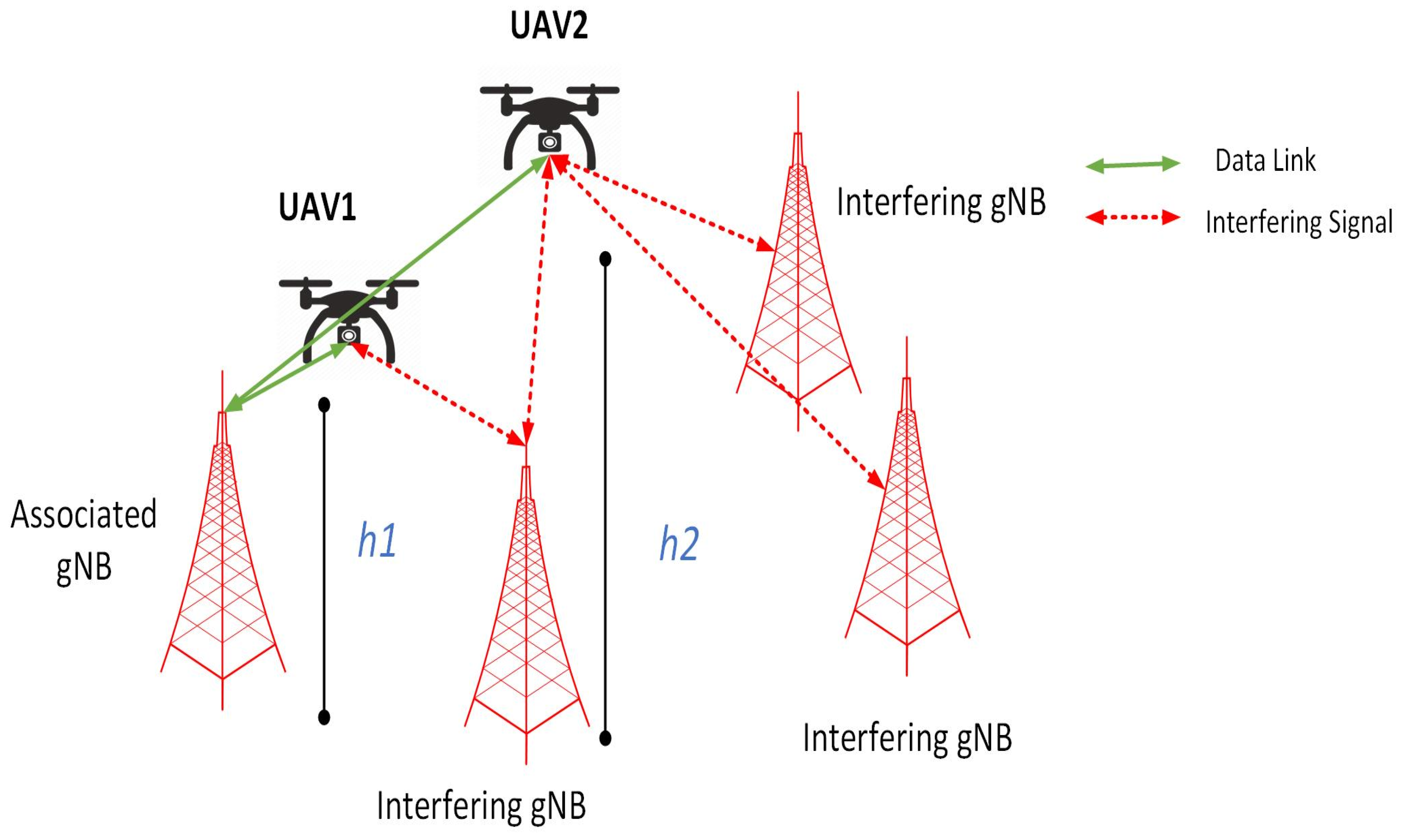
Figure 2 illustrates aerial interference in a 5G network. Specifically, it highlights the impact of height on interference for two UAVs, namely UAV1 and UAV2, which fly at altitudes
and
, respectively. UAV1 experiences severe interference from a neighbouring gNB, whereas UAV2, flying at a greater altitude (
), faces interference from three neighbouring gNBs due to the presence of favorable LoS links. This observation suggests that higher altitude leads to interference from all neighbouring gNBs due to the existence of favorable LoS links. During downlink communication, each UAV experiences interference from multiple neighbouring gNBs that are not associated with it due to strong LoS channels, resulting in poor downlink performance. In uplink communication, the UAV creates significant interference for several adjacent non-associated gNBs, thereby causing a new gNB interference problem. Although resource block (RB) allocation is a common approach for addressing this issue, it is ineffective for severe air–ground interference. This is because of the limited number of RBs available to UAVs and the high frequency reuse for terrestrial UEs in cellular networks. Thus, developing an interference mitigation technique that accounts for the unique channel and interference characteristics of cellular-connected UAVs is critical. Although current terrestrial mitigation strategies can partially mitigate air–ground interference, severe interference cannot be entirely eliminated. This paper presents an interference mitigation algorithm that is designed exclusively for downlink scenarios involving 5G-connected UAVs.
The objective of this research paper is to devise a new approach to power control that can mitigate interference in 5G networks, specifically addressing the challenges associated with the use of UAVs. To accomplish this, we put forward the utilisation of the DQL algorithm as a means of mitigating interference in power control.
5. Reinforcement Learning
Reinforcement learning (RL) is a specialised area within the realm of machine learning that concerns itself with determining appropriate actions to be taken by an intelligent agent in a given environment. The objective of this methodology is to maximise the cumulative reward obtained by the agent by selecting the most optimal action. It places emphasis on finding a balance between exploration and exploitation, thereby continually refining the agent’s decision making capabilities. The agent must actively gather information about possible states, actions, transitions, and rewards. Unlike supervised learning, where evaluation is separate, in RL, the agent is evaluated while learning. The agent interacts with the environment through perception and action. The agent receives input in the form of the current state of the environment and selects an action to alter the environment’s state. The agent then receives a scalar reinforcement signal or reward based on the value of the state transition. The agent’s goal is to maximise the long-run sum of the reinforcement signal’s values by selecting actions that tend to increase the reward.
Table 2 provides definitions for various elements involved in the training phase that determine interaction between the agent and states and provide expected discounted reward value.
Figure 7a illustrates inter-element interaction. The agent changes its state from
s to
by taking an action
a in an environment and receives reward
w for it.
In this work, the agent is the DQL algorithm, which exists in a given state
s, i.e., a specific power value. It takes a suitable action, i.e., increase or decrease the power value, to optimise the SINR value. This interaction takes place in a 5G cellular environment. Finally, these commands are sent to the UAV. This is depicted in
Figure 7b.
5.1. Q-Learning
Q-learning is a commonly used reinforcement learning algorithm for making optimal decisions in Markov decision processes (MDPs). In Q-learning, the agent learns a Q-function that maps a state–action pair to a value representing the expected cumulative reward obtained by taking that action from that state and following an optimal policy thereafter. Thus, the Q-table is the mapping of state–action pairs with a Q-value relating to the reward.
Table 3 illustrates a Q-table.
The Q-value is not calculated in a fixed manner; instead, it is implemented in the Q-table as an iterative approach. This is known as the training phase.
The Q-table is a fundamental component in the Q-learning algorithm, serving as a means of storing and updating information regarding the states, actions, and their associated expected rewards. It is implemented as a mapping between state–action pairs and their corresponding Q-values, which represent the estimated optimal future rewards of taking a particular action from a specific state.
The Q-learning algorithm works through the following steps:
Initialise Q-table: At the initiation of the Q-learning process, the Q-table is initialised to an array of zeros, indicating a lack of prior knowledge about the environment. As the agent interacts with the environment through trial and error, it updates its understanding of the state–action pairs and their corresponding Q-values, which it uses to optimise its future actions and maximise its expected reward.
Choose an action: To choose an action in Q-learning, the agent can use an exploration–exploitation strategy. During the exploration phase, the agent randomly chooses actions to gain information about the environment. During the exploitation phase, the agent chooses actions based on its current estimate of the optimal action-value function. One common exploration–exploitation strategy is the epsilon-greedy strategy. The agent chooses a random action with probability , and the optimal action (i.e., the action with the highest Q-value) with probability . As the agent gains more experience, it can gradually decrease the value of , which allows it to explore less and exploit more.
Update Q-table: The Bellman Equation is a mathematical expression that facilitates the determination of updates to the Q-table following each step taken by the agent. The equation effectively integrates the current perception of value with the anticipated optimal reward, which is premised on the selection of the optimal action as known at that moment. In a practical implementation, the agent assesses all feasible actions for a given state and chooses the state–action pair with the maximum Q-value. The Bellman Equation [
31] is formulated as in (
1).
Here,
.
is the next state.
is the next action. These steps are repeated until the optimal solution is converged. This is also represented in
Figure 8.
In this paper, Q-learning for interference mitigation is considered the baseline method against which the proposed algorithm is compared.
5.2. Deep Learning
Deep learning algorithms use gradient descent optimisation and back-propagation to iteratively adjust the weights of the network and improve its predictions, with the goal of minimising the prediction error on the training data. The hierarchical representation learning in deep learning enables the model to learn increasingly complex features and representations, leading to its widespread use in numerous applications, including natural language processing, computer vision, and speech recognition. The depth and number of layers in deep learning models can vary, ranging from simple feed forward networks to complex recurrent neural networks and convolutional neural networks [
42].
A neural network (NN) is an AI model composed of interconnected neurons or activations arranged in multiple layers. The NN transforms input data into output data based on a pre-established training dataset. This mapping is accomplished through the distribution of adjustable parameters known as weights across the various layers. The weights are refined through the use of the back-propagation algorithm, which minimises a loss function that gauges the deviation between the network’s predictions and actual values. To reduce the loss function (or to optimise the back-propagation algorithm), gradient descent is used. In the mathematical theory of neural networks, universal approximation theory establishes the density of an algorithmically generated class of functions. Therefore, if (f(x)) is an arbitrarily complex function, then the neural network can approximately approach the solution of the function irrespective of its type. This implies that neural networks are capable of representing a wide variety of functions when given appropriate weights [
43]. Activation functions help NNs differentiate between useful and irrelevant data points.
5.3. Neural-Network-Based Function Approximator
If the initial state–action value function is modified for every time instant ‘t’, then it will converge to as . However, this is not easy to achieve. The primary cause for this is due to its implementation in a non-stationary environment. Real-world environments, such as the 5G-UAV integrated network considered in this paper, are often dynamic and may change over time. In such environments, the optimal policy itself may change, making it difficult for the algorithm to converge. Frequent updates of the state–action values can exacerbate this issue as the learning process might not be able to keep up with the changes in the environment. To counteract this, we use a function approximator.
At a given time, a neural network with its weights is defined as . Also, if is defined, a function approximator ≈ is constructed.
This neural-network-based function approximator forms the DQN. An important component of neural networks is activation functions. The sigmoid function, as shown in (
2), is a popular choice [
31] for the activation function. The sigmoid function is a mathematical function that maps any real-valued number to a value between 0 and 1. It is defined as
The deep network is trained by modifying
for every
t to reduce the mean-squared error loss represented by
:
where
+
is the approximate value of the function at t, when the current state is
s and action
a. Interacting with the environment in this manner and making a prediction, comparing it against the correct response, and suffering a loss
is termed online training. The associated gNB relays the UAVs’ feedback data to a central location for DQN training in online learning [
31].
The dimension of the input layer is the no. of states |
|, while the output layer is set to the no. of actions
. A small depth is chosen for the hidden layer as it has a direct impact on the computational complexity. This is shown in
Figure 9.
5.4. Deep Reinforcement Training Phase
Stochastic Gradient Descent
During the training phase, the weights are subject to iterative modifications employing the Stochastic Gradient Descent (SGD) technique. SGD represents a variant of the gradient descent method, wherein a differentiable (or sub-differential) function is optimised through stochastic approximation. This is achieved by substituting the actual gradient, computed from the complete dataset, with an estimated gradient derived from a randomly selected minibatch of the dataset. By adopting this approach, particularly in optimization problems characterised by high dimensionality, the computational burden is mitigated, resulting in accelerated iterations.
During the training phase, the weights
are subject to modification following each iteration of time, achieved through the utilisation of the SGD method on a selected minibatch of data. It starts with an initial value of
, which is chosen at random, and iterates and updates this value using an
step size as follows:
The training is supported by replaying the experience from a replay buffer
.
stores the different experiences
from different episodes at each time step.
is defined in (
5)
Subsequently, random samples were drawn from the dataset and organised into minibatches. The training process is then conducted on these minibatches of data. This approach offers stability and mitigates the risk of convergence to local minima. As a result, the parameters used to generate the sample from differ from the current parameters of the deep neural network.
The state–action value function
estimated by the deep Q-network (DQN) is defined by Equation (
1).
5.5. Policy Selection
Q-learning is a type of off-policy reinforcement learning algorithm, which allows for the creation of a nearly optimal policy even if actions are selected based on a random exploratory policy. As a result, a nearly greedy action selection policy is adopted, consisting of two modes.
Exploration: In the beginning, when the agent is unaware of the most effective action, it tries different actions randomly to determine an effective action
Exploitation: Once the agent learns the various actions, it then chooses an action based on this knowledge to maximise the state–action value function .
According to this policy, where is a hyperparameter, regarding the trade-off between exploration and exploitation:
- (i)
the agent carries out exploration with a probability .
- (ii)
probability is used for exploitation.
The trade-off results in this policy being referred to as -greedy action selection policy. This policy has a linear regret in t.
In the system model adopted in this work, it is assumed that UAVs move at speed v and the agent selects from its and receives and finally moves to . An episode is the time period in which the agent and environment interact. If the target is achieved within the episode, then it is said to have converged.
In the proposed DQN implementation, the UAV coordinates are particularly kept track of. These coordinates are reported to the network and used for decision making to improve the network performance. Thus, UAV coordinates are part of the DRL framework.
5.6. Hyperparameter Tuning Using Random Search
Hyperparameter tuning is required for the proposed DQL algorithm to achieve better performance and stability during the training process. In this work, we use the random search technique to effectively tune the hyperparameters.
Random search is a simple and intuitive hyperparameter tuning technique widely used in machine learning and deep learning. Its primary goal is to find optimal hyperparameter configurations that maximise the performance of a model in a given task. Random search samples hyperparameter values randomly from predefined ranges. The process of random search involves defining a search space for each hyperparameter, typically specified by minimum and maximum values. During each iteration, the algorithm selects random values for each hyperparameter from their respective search spaces. These randomly sampled hyperparameter configurations are then used to train the model. The random search method is implemented similar to [
31] as the environments used in their work are similar to ours. Random search entails the following steps:
Define search space: This is a range of possible values to sample from for each hyperparameter, i.e., learning rate (), discount factor (), and exploration rate ().
Initialise optimal hyperparameters: Before the random search begins, we initialise the hyperparameters to an initial value. In the proposed algorithm, a maximization problem is considered; therefore, the initial values are set to a very low value. After, this random search is performed.
Train the DQL agent with sampled hyperparameters: Using the sampled values obtained after the random search, the DQL agent is trained within the environment until convergence.
Evaluate the performance: Evaluate the agent’s performance by running the agent in the environment for a fixed no. of episodes. Compute the average reward as given by expression in
Table 2 as a performance metric.
Update the optimal hyperparameters: If the values of hyperparameters after random search are better than initial optimal values, then the optimal values are updated to current values.
The optimal hyperparameter values obtained from this method are provided in
Table 4.
7. Network, System, and Channel Model
7.1. Network Model
In this scenario, a cellular network with gNBs is analysed. Each network consists of one associated gNB and at least one interfering gNB, and the UAVs’ association with their associated gNB is based on their distance. A UAV can only be served by one gNB at a time, so the cell radius can be expressed as .
7.2. System Model
Under the given network model and considering a multi-antenna setup, with each gNB equipped with M antennas and each UAV having a single antenna, the signal received at the UAV from the
-th gNB can be expressed as
Here,
,
are transmitted signals from the
th and
th gNBs, and it meets the power constraint
The vectors , and are channel vectors representing the connection between the UAV and the -th gNB, and the connection between the UAV and the -th gNB, respectively. Finally, is drawn from a complex normal distribution with zero mean and variance of , representing the noise received by the UAV.
The first term in Equation (9) represents the desired signal received by the UAV, while the second term represents the interference received from non-associated gNBs.
Each gNB transmits power from the set of all possible power values, denoted by . This set is defined such that the possible transmit power is a power offset.
7.3. Channel Model
In order to delineate the conditions of signal propagation, the concept of LoS probability is introduced to quantify the likelihood of the LoS component’s presence. The 3GPP channel model [
45] provides specific LOS probability models, with antenna heights of 3 m for indoor scenarios, 10 m for Urban Micro (UMi) environments, and 25 m for Urban Macro (UMa) settings. With respect to this work, the UMa scenario is chosen. This can be written as
where
Pathloss presents a strong correlation with the channel modelling and is influenced by distance. Since UAVs operate in a three-dimensional environment, the pathloss is given by
where
is the location of the UAVs 3D distances and
is the operating frequency.
This algorithm adopts a narrow-band geometric channel model, as described in [
12]. With this model, the downlink channel from gNB
to the UAV in gNB
can be expressed as
where
: path gain of the p-th path;
: angle of departure(AoD);
: array response vector associated with AoD;
: no. of channel paths.
This model accounts for both LOS and NLOS scenarios. For the LOS case, is assumed.
The received power at the UAV is measured over a set of PRBs at a given time
t and is given by
where
is received downlink power,
is power from gNB
.
Some additional losses are also suffered due to penetration and oxygen absorption.
8. Simulation Set-Up and Results
In the system model considered in this paper, a UAV is operating within the range of 2 gNBs in a 5G-RAN network. One gNB is associated with the UAV and the other one is the interfering gNB. The UAV sends its measured SINR to the gNB, which is then served as the input to the DQL algorithm. The SINR received by the UAV served in gNB
at time
t is computed as follows
This is the received SINR that will be optimised by the proposed DQL, which is located in the cloud, linked to the RAN. The output of the DQL is then fed back to the gNB. The gNB then sends these commands back to the UAV, which optimises the SINR and mitigates interference.
8.1. Simulation Setup
The network, system, and channel models have been detailed in prior descriptions. The UAVs are in motion at a velocity of ‘v’ and are subject to the impact of log-normal shadow fading and small-scale fading on their movement. The radius of the cell is denoted as ‘r’, and the inter-site distance is established as R = 1.5r. The channel conditions of the UAVs are influenced by a probability of LoS denoted as
. The remaining parameters are presented in
Table 4. The target effective SINRs for the objective are specified as
where
is the established SINR. If the
drops below a minimum of −3 dB, the episode is considered to have concluded and the session cannot proceed any further.
The hyperparameters used to tune the RL-based model are shown in
Table 4.
Table 6 summarises the radio parameters.
The simulated states
are set up as
where (x,y) are the Cartesian coordinates (i.e., longitude and latitude) of the given UAV.
By leveraging the cardinality of
, which scales in the order of 2, the set of actions
can be derived. Specifically, a register
a is utilised to facilitate a binary encoding of the available actions. With the aid of masks, bitwise-AND operations, and shifting, the power control commands can be obtained. The code segment as shown in
Table 7 is adopted:
When q = 0:
It can be inferred from above that = (±1, ±3) dB offset from the transmitter power. The following factors affected the choice of these offset values:
It conforms to the standards [
46] that select integers for power value increments.
It maintains the non-convexity in (8) because it keeps the constraints discrete. Actions that increase or reduce gNB transmit powers are implemented as in [
30].
A function
is defined that returns an element from
depending on the selected code. In this work, it is considered that p(00) = —3, p(01) = —1, p(10) = 1, p(11) = 3. The received SINR resulting from the above actions can, therefore, be written as
We thus write the reward as
where
q = 0.
The agent is rewarded the most when it triggers a power control command. The episode is aborted when the constraint imposed on (8) becomes inactive. In this scenario, the agent receives a reward along with one of the following:
In the simulations, the following steps are taken:
Minibatching is performed with a sample size of 32 training samples.
The width of the DQN can be found as per [
47]. Thus, (22) is written as
Substituting for |A| = 16 and , we obtain H = 24.
The following performance measures are used to benchmark our algorithms:
Convergence (ζ): Defined as the episode at which the is satisfied over the duration T for all UAVs. It is expected that, as the no. of UAVs h increases, will increase. For several random seeds, an aggregated percentile convergence episode is taken.
Runtime: Determining the runtime complexity of the proposed DQL algorithm is difficult due to the absence of guarantees for convergence and stability. Therefore, runtimes from simulation per UAV are considered.
Coverage: A complement cumulative distribution function (CCDF) of is built by changing the random seed and performing the simulation in iterations, effectively modifying the way the UAVs drop from the network.
The proposed DQL overcomes the shortcomings of FPA by implementing an adaptive power control scheme that can accommodate the changing interfering conditions. Tabular Q-learning relies on the initialised state–action value function, which is fixed. This results in the size of the Q-table becoming quite large and therefore taking longer times to find the optimal solutions, thus resulting in longer convergence time. However, in the proposed DQL, the neural network implementation eliminates the need for a Q-table, instead updating the optimal actions in real time.
8.2. Results
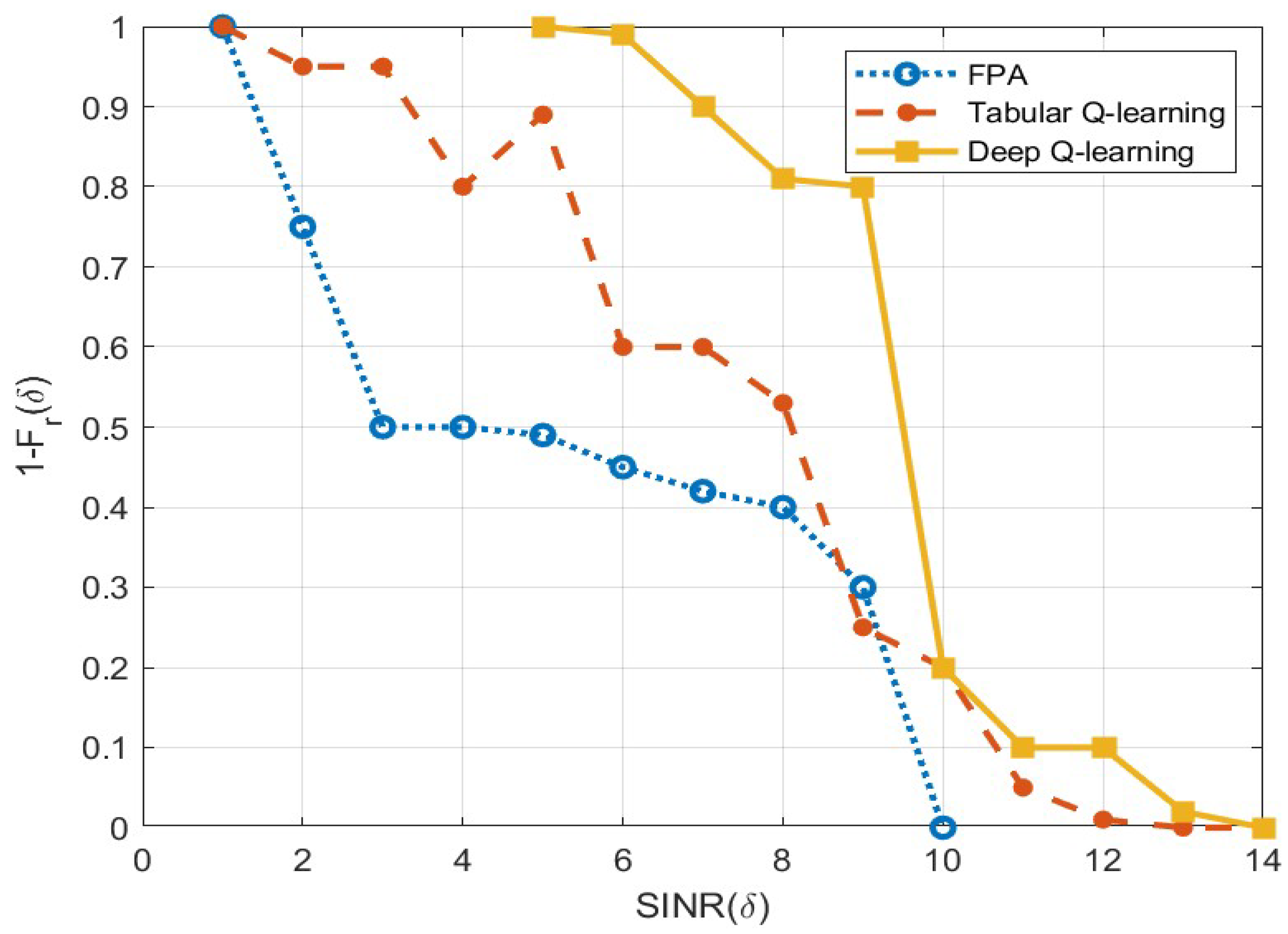
Considering the episode with the highest possible reward,
Figure 11 shows the plot of the Cumulative Complement Distribution Function (CCDF) of
, shown for the three algorithms FPA, tabular Q-learning, and the proposed DQL.
As anticipated, the FPA strategy produces the least optimal performance due to its lack of power control or interference coordination. Tabular Q-learning exhibits slightly improved results over FPA, yet it still falls short when compared to the addition of power control mechanisms to the gNBs, under-performing FPA at approximately dB. On the other hand, the proposed DQL algorithm outperforms the other two algorithms, achieving better convergence to a solution. Unlike the tabular implementation, the convergence of DQL is not affected by the initial state–action value function. As approaches 13 dB, UAVs are situated in closer proximity to the gNB, resulting in comparable performance among all power control algorithms.
We also analyse the link performance for each of the algorithms at different heights of the UAV. As explained in the previous sections, when the altitude increases, the interference also increases.
The simulation is run for a duration of 120 s, with the UAVs flying at three different altitudes: 50 m, 100 m, and 120 m. To analyse the link performance, SINR and latency are compared for the different heights and the three different interference mitigation schemes.
8.2.1. UAV @ 50 m
In this section, we discuss the results when the UAVs are flying at a height of 50 m. This is a relatively lower altitude; therefore, the number of interfering elements is relatively lower.
Figure 12 shows SINR values for UAV @ 50 m. When no link adaptation is employed, i.e., when the FPA method is used, the values vary from
to
. This is a relatively steady performance; however, the SINR values are the lowest compared to Q-learning and DQL. This is expected as it is a lower altitude and the interference conditions do not change drastically, except for a brief 27 s peak between the 26 s and 53 s marks. Q-learning starts with a higher value of 9.7 dB and even goes up to 11.6 dB with an average value of 10.45 dB. This is indicative of good performance for the link; however, after about 95 s, it suffers a drastic dip in performance in addition to presenting erratic patterns till the end of the simulation. This can be seen in
Figure 12 as the annotated text in the red circle. When the simulation progresses, the Q-table becomes large and achieving the optimal solution becomes difficult. This is also reflected in the link latency as shown in
Figure 13.
Finally, DQL performs the best with average, minimum, and maximum values of 12.06 dB, 11.74, and 12.19 db, respectively, which is indicative of steady performance with high SINR values. It also shows a really low latency value of 25.61 ms. Consequently, interference is best mitigated by DQL amongst the three methods.
8.2.2. UAV @ 100 m
In this section, we discuss the results when the UAV is flying at a height of 100 m. This is a higher altitude; therefore, the number of interfering elements is relatively higher.
Figure 14 shows SINR values for UAV @ 100 m. When no link adaptation is employed, i.e., when the FPA method is used, the values vary from
to
. This represents an unstable link as the SINR values vary drastically. For example, at about the 32 s mark, there is an increase to 6.95 dB from 6.5 dB, but, from thereon, it drops sharply to reach its minimum possible value. It increases again and does not stay constant. As mentioned above, this is primarily because the FPA algorithm cannot take into account the changing interference conditions, and, at a higher altitude of 100 m, the increase in interfering elements leads to a change in the interference conditions. This also coincides with the latency values, which see delays of up to 55 ms, as shown in
Figure 15.
Q-learning starts with a lower value of 7.74 dB as compared to its 50 m performance. It maintains a steady performance value of close to 8.8 dB till about 88 s. This is indicative of good performance for the link; however, after about 89 s, it suffers a drastic dip in performance and undergoes a series of peaks and troughs till the end of simulation. At one point, specifically at the 104 s mark, it falls even below the FPA values. This can be seen in
Figure 14 as the annotated text in the red circle. When the simulation progresses, the Q-table becomes large and achieving the optimal solution becomes difficult. This is also reflected in the link latency as shown in
Figure 15.
Finally, DQL performs the best with average, minimum, and maximum values of 10.51 dB, 9.74 dB, and 10.633 dB, respectively, which is indicative of steady performance with high SINR values. It also shows a really low latency value of 34.01 ms. Even though it shows a 12.58% decrease in SINR values and 32.6% increase in latency values as compared to 50 m, it is still the best-performing algorithm. It implements link adaptation absent from FPA and eliminates the need for Q-tables by the use of neural networks.
It is to be noted that the overall performance of the UAV at 100 m deteriorates as compared to 50 m. The main cause for this is the fact that, due to the higher altitude, the number of interfering elements, i.e., gNBs that UAV has LoS with, increases.
8.2.3. UAV @ 120 m
In this section, we discuss the results when the UAV is flying at a height of 120 m. This is the highest altitude under consideration; therefore, the number of interfering elements is the maximum amongst the considered scenarios.
Figure 16 shows SINR values for UAV @ 120 m. When no link adaptation is employed, i.e., when the FPA method is used, the values vary from very
to
. This represents an unstable link as the SINR values vary drastically. For example, at about the 31 s mark, there is a sharp drop to 1.45 dB from 5.05 dB for about 30 s. However, at the 73 s mark, it increases till 5.38 dB sharply in a 6 s duration before falling back to 41.38 ms by the end of 100 s, after which it increases again and does not stay constant. The periods of steady and stable values are lesser as compared to when the UAVs are at a lower height, for example, between 0 and 26 s, and between 67 s and 73 s. As mentioned above, this is primarily because the FPA algorithm cannot take into account the changing interference conditions and, at a higher altitude of 100 m, the increase in interfering elements leads to a change in the number of interfering elements. This also coincides with the latency values, which see delays of up to 67.447 ms, as shown in
Figure 17.
Q-learning starts with a lower value of 5.78 dB as compared to its 100 m performance. It maintains a steady performance value of close to 6.8 dB till about 88 s. This is indicative of good performance for the link; however, after about 89 s, it suffers a drastic dip in performance and undergoes a series of peaks and troughs till the end of simulation. When the simulation progresses, the Q-table becomes large and achieving the optimal solution becomes difficult. This is also reflected in the link latency, as shown in
Figure 17.
Finally DQL performs the best with an average, minimum and maximum values of 8.51 dB, 7.72 dB and 8.6354 dB respectively, which is indicative of steady performance with high SINR values. It also shows a really low latency value of 43.15 ms. Even though it shows a 15.58% decrease in SINR values and 26.87% increase in latency values as compared to 100 m, it is still the best best performing algorithm. It implements link adaptation absent from FPA and eliminates the need for Q-tables by the use of neural networks.
It is to be noted that the overall performance of the UAV at 120 m is the worst as compared to 50 m and 100 m. The main cause for this is the fact that, due to the higher altitude, the number of interfering elements, i.e., gNBs that UAV has LoS with, increases.
Figure 18 shows the SINR values for three different speeds of the UAV. It is seen that, with increasing speeds of the UAV, it does not see any drastic changes in SINR values. The average
value falls from about 9.5 dB at 10 m/s to 8.5 dB at 30 m/s. This is a clear indication that the DQL algorithm deals well with high speeds of the UAV.
Table 8 summarises the results with different speeds.
Figure 19 shows the observed normalised runtime. Compared to FPA and tabular Q-learning, the proposed DQL algorithm has a shorter runtime and performs better in terms of convergence and capacity. As the no. of UAVs h increases, the runtime complexity of FPA and tabular Q-learning increase rapidly, but the runtime of DQL remains relatively low. At h = 4, the DQL algorithm only took 4% of the runtime of the other two algorithms. This behaviour is observed because the increase in h means that the number of interfering elements increases. FPA and tabular Q-learning are not able to accommodate these changing interfering conditions effectively, but the proposed DQL performs better than them.
Another way to visualise and evaluate an agent’s performance during its training process is the reward plot.
Figure 20 shows the reward plot for the proposed DQL method. As expected, the rewards are low in the beginning as the agent is learning to find the best solution, but they increase as the episodes progress, as the agent learns the best solution and keeps leveraging that knowledge as the proposed model employs an epsilon greedy policy.
8.3. Outcomes
In this section, the outcomes of the performance measures are presented:
Convergence: We observe normalised convergence under (17), where = 5 dB. Each time step is equal to one radio sub-frame, with a duration of 1 ms. With an increase in the number of “h”, the number of episodes necessary to achieve convergence also increases, with little to no impact on the threshold. since .
Runtime: The normalised runtime is observed. As h increases, the complexity of runtime complexity also increases for the proposed algorithm. This is justified because of an increased number of interfering elements.
Coverage: Coverage is defined by , which evidently improves everywhere. Coverage improves where increases monotonically.
Additionally, the proposed solution is compared against some of the state-of-the-art methods implemented in the environment used in our work. The following
Table 9 summarises the results. It is observed that the proposed DQL is considerably better than the other methods. SINR sees a 41.66% increase while using DQL as compared to mean-field game theory, the next best algorithm.
In
Figure 21, we plot the average SINR values of different methods as well as the proposed method and observe that the proposed method performs better than the existing methods in effectively mitigating interference. This can be explained by the following reasons: convolutional neural networks (CNNs) often require large memory spaces to store the weights and activations of the convolutional layers; this results in large overhead and complex design as opposed to the proposed DQL. Mean-field Q-learning has scalability limitations, unable to cope with a large number of agents and the consequent large growth of the action space. Particle swarm optimization can also be used for power allocation to mitigate interference. However, this method is designed to exploit the best solutions in the search spaces to a global optimum, which may not be the best trade-off between exploration–exploitation. Mean-field game theory for interference mitigation is also one of the methods amongst the existing works. However, this method is computationally complex, expensive, and challenging.


