Abstract
This study was designed to identify trends in maximum, minimum, and average air temperatures in the Federal District of Brazil from 1980 to 2010, measured at five weather stations. Three statistical tests (Wald–Wolfowitz, Cox–Stuart, and Mann–Kendall) were tested for their applicability for this purpose, and the ones found to be most suitable for the data series were validated. For this data sample, it was observed that the application of the Wald–Wolfowitz test and its validation by the Cox–Stuart and Mann–Kendall tests was the best solution for analyzing the air temperature trends. The results showed an upward trend in average and maximum air temperature at three weather stations, a downward trend at one, and the absence of any trend at two. If the trend of increasing air temperature in the Federal District persists, it could have a negative impact on various sectors of society, mainly on the health of the population, especially during the dry season when more cases of respiratory diseases are registered. These results could serve as inputs for public administrators involved in the planning and formulation of public policies.
1. Introduction
Some climatic factors are perceived by society in a very peculiar way, as they imply a series of daily sensations such as heat or cold, lack of or excessive rainfall, and strong winds. These perceptions of atmospheric weather are invariably associated with and mistaken for climatic aspects, since by their very nature they influence individual perceptions of environmental comfort on a daily basis. Therefore, studying the climatic data elements and their variations is relevant to society.
Considerations such as the thermal comfort of buildings or the potential for weather to cause illness must be based on short-, medium-, and long-term observations, because while immediate analyses can help guide emergency actions, long-term data series are essential for understanding temporal and spatial dynamics in order to support socio-environmental planning.
A plethora of meteorological data is now produced around the world. However, in its diversity it can sometimes induce readers—no matter how well-informed they are—to misapprehend the difference between weather and climate due to differences in their presentation and especially different interpretations of variations in climatological parameters.
With this concern in mind, Jones and Moberg [1] revised the air temperature databases of ground stations of the Climate Research Unit (CRU) in seven continents and the Arctic in order to take account of technological advances in data collection and dissemination methods and the emergence of initiatives by countries and research institutions to increase the quantity and quality of data. The results showed that the hemispheric and global air temperature averages yielded by the new data set differ slightly from those developed in 1994, leading to the conclusion that periodically updating the time series database of climatic data is essential for effective research.
One factor that should be paid attention to when analyzing time series in the science of climatology is the source of data, given that meteorological stations can be located in homogeneous and/or heterogeneous environments. As a rule, the distinction between these spaces is centered on the distinction between urban and rural landscapes; however, Stewart and Oke [2] emphasize that it is important to be aware of the distinct characteristics within each such landscape (rural and urban), meaning greater care is needed when considering them as objects of scientific analysis.
This observation is relevant because of the great diversity of applications and uses of the terms “urban” and “rural,” not to mention the structural elements of landscapes, especially urban ones. This consideration is brought into focus in studies of urban heat islands [3,4,5,6,7,8,9,10,11,12].
In climatology, it is a consensus that urban and rural spaces differ in their values of measurement of meteorological parameters, in particular, where air temperature and relative humidity are concerned. This is one of the targets of study of urban climatology. Skarbit et al. [13] analyzed the average annual and seasonal air temperature conditions in the local climate zones (LCZs) of Szeged, Hungary. The basis of the analysis was a one-year dataset from 2014 to 2015 from a 20-station urban meteorological network. The network and its corresponding LCZs put air temperature studies in Szeged into a new spatial framework to assess local climate and urban heat island conditions.
The results showed that densely built-up LCZs have a higher annual and monthly average, and minimum air temperatures than structurally open and more vegetated classes, with nocturnal differences of >4 °C observed under a calm, clear sky. Among the air temperature indices measured in the urban LCZs, frosty days, cooling degree days, and tropical nights were found to differ markedly from the background rural LCZs. This difference suggests that local climatologies exist within Szeged, which have implications for thermal comfort, urban energy use, and urban agriculture.
In Brazil, this phenomenon has also been observed. In tropical environments, where there are situations of thermal stress, thermal discomfort is particularly aggravated by urban heat islands [14,15,16,17]. Amorim [18] also points out that intra-urban characteristics can intensify high air temperature events. Therefore, it is important to consider the local specificities and particularities of each urban agglomeration and its neighboring areas, as indicated by [19], when presenting a proposal for the classification of climate zones for urban areas.
Stewart and Oke [19] developed a classification focused on the landscape, which was evaluated as a whole then broken down according to surface changes. Amorim et al. [12] points out that Oke [20] understands the importance of defining climate zones not because of their absolute precision in describing a location, but because of their ability to classify the urban areas of a neighborhood into sectors with a similar propensity to modify the local climate.
The analysis of meteorological time series can also be enhanced by trend analysis. The detection, estimation, and prediction of trends are important aspects of climate research [21,22]. In any given time series, the trend is the rate at which a parameter changes over a period of time. By evaluating trends, it is possible to ascertain the prevailing direction of a given numerical variable. What is sought from a time series are the movements and directions of specific variables, which, in the case of the present investigation, is the air temperature in the Federal District of Brazil from 1980 to 2010.
Minuzzi et al. [23] used statistical methods to analyze the patterns of seasonal and annual rainfall and dry spells at 21 hydrological stations located in Paraná, southern Brazil. Silva [24] studied the variation of evapotranspiration in Acre, Brazil, in order to understand its spatial and temporal variability and identify possible trends. Gomes et al. [25] identified trends in the annual average maximum air temperature series for western Pará, Brazil, from 1980 to 2013, using the Mann–Kendall test. The results show that annual average maximum air temperature increased over time, mainly in the winter.
A significant number of researchers working in different regions of the globe on different spatial scales have investigated trends in climatic variables. What these studies all agree on is the need to monitor basic data so that these trends can be ascertained with precision and accuracy, making use of all available statistical resources, providing more effective inputs for public administrators and planners [26,27,28,29].
In Brazil, urban climate and climate trend research in the Federal District is still incipient. Ribeiro [30] analyzed the impacts of urban expansion on the variation of meteorological elements in the area in order to identify heat islands in specific sectors. Baptista [31] carried out a study on heat islands in the Federal District based on Landsat 5 TM images, detecting an average increase of 3 °C in air temperatures from 1984 to 2001.
Steinke et al. [32] studied the variation in air temperature in five weather stations in the Federal District. In this study, data from a 38-year period (1965–2013) were used to study the trends in maximum and minimum temperatures. The data were analyzed using a non-linear regression model. The estimated curves for each year were compared with the non-linear adjustment of climate normals (1961–1990) of average monthly air temperature. The results showed that although positive anomalies were observed in the average air temperature in the late 1990s, the existence of an upward trend could not be ascertained in the period.
The Federal District is situated in the central region of Brazil. The capital city, Brasília, which was built sixty years ago, is its main urban hub. As already mentioned, studies involving air temperature in this region are still scarce. Therefore, this territorial section of the Federal District of Brazil could be an excellent laboratory for studies of local/regional climate in tropical environments whose original landscapes have been altered by anthropic action in the last century.
These considerations are consistent with the broader purpose of this study, which is to determine the best statistical method for ascertaining the existence of trends in a time series of air temperature data from weather stations located in areas subject to different types of land use in the Federal District, Brazil, from January 1980 to December 2010.
2. Materials and Methods
The socio-environmental aspects of the Federal District are widely characterized in the literature [33,34,35,36], as are the region’s climatic characteristics [32,37,38,39]. The atmospheric circulation systems associated with the geographical position of the Federal District define two periods: a dry, cool period stretching from late April to September, and a warm, rainy period running from late October to late March.
This study analyzed the monthly time series of the minimum temperature (Tmin), average temperature (Tav), and maximum temperature (Tmax) of the air at five meteorological stations in the Federal District (Figure 1). The weather stations are located in urban and rural areas: two in urban areas (National Institute of Meteorology (INMET) and Integrated Center for Air Defense and Air Traffic Control (CINDACTA)), two in predominantly rural areas (Embrapa Hortaliças (CNPH) and Embrapa Cerrados (CPAC)), and one in a transition area between urban and rural areas (Fazenda Água Limpa (FAL-UnB)), situated in a farm whose borders have been the target of urban expansion. Figure 2 shows the detailed location of the weather stations.
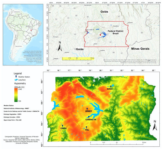
Figure 1.
Spatial distribution of weather stations in the Federal District, Brazil.
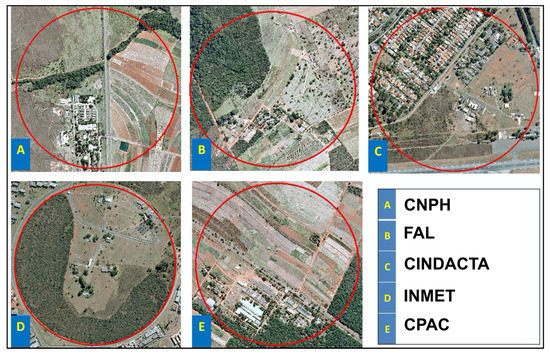
Figure 2.
Details of the location of the weather stations.
Data Set Analysis
The present study used time series of air temperature data to indicate whether or not there was an upward trend in this parameter. Continuous time series are obtained by recording observations continuously over a particular time interval.
The tests for trend analysis in time series are intended to build models. Two approaches can be used for this type of analysis: either using parametric tests, which have a finite number of parameters, or using frequency domain, which is non-parametric. This latter analysis is widely used in meteorology to assess the periodicity of phenomena [40].
According to [41], parametric tests are more accurate and their validation is based on more assumptions. In non-parametric tests, the original values are replaced by a ranked order of values to calculate their statistics and are independent of the probability distribution of the data studied.
Non-parametric tests are recommended for detecting trends in climatological data due to the original characteristic of these data, which do not have a normal frequency and present positive asymmetries [42]. In the present study, three non-parametric statistical tests that are widely used to assess trends in time series, especially of climatological data, were investigated: the Wald–Wolfowitz runs test, the Cox–Stuart test, and the Mann–Kendall test. Monthly data from 1980 to 2010 were used, producing time series of minimum, maximum, and average air temperatures from five weather stations. Statistical tests were performed using the statistical software package R.
Wald–Wolfowitz Test: The Wald–Wolfowitz runs test checks a hypothesis of randomness for a two-valued data sequence. More precisely, it can be used to test the hypothesis that the elements in the sequence are mutually independent. For this test to be used, the time series must be independent and very well distributed, as follows:
Let {Zt, t = 1, …, N} be a time series with N observations. Consider M to be the median of N observations of Zt. Each value of Zt is assigned the symbol “a” if it is greater than or equal to M, and “b” if it is less than M. Therefore, N = (“Na” points “a”) + (“Nb” points “b”). Accordingly, there are groups of observations marked with “a” and groups of observations marked with “b” throughout the time series. The total number of groups will be the test statistics, that is:
- T = total number of groups with identical symbols.
Consider the following hypotheses:
- H0 = there is no trend;
- H1 = there is a trend.
The null hypothesis, H0, is rejected if there is a small number of groups with identical symbols, that is, if T is relatively small. For Na and Nb values of over 20, it is possible to use the Central Limit Theorem and ascertain the approximate distribution of T by a normal distribution, that is,
T ~ N (μ, σ ^ 2), where:
The Wald–Wolfowitz runs test has been used for numerous applications [43,44,45], including trends in time series of climatic data. This test, described in detail by [46,47], is designed to identify the hypothesis of independence of data values.
Cox–Stuart test: Cox and Stuart [48] proposed a way to test upward or downward trends, which do not necessarily have to be linear, but can simply express an overall trend in the observations. The Cox–Stuart test has been defined as having limited power, but very robust for trend analysis [49]. It is applicable to a wide variety of situations to get an idea of the overall evolution of the values obtained. The method is based on binomial distribution.
In the Cox–Stuart test, considering a set of observations X1,x2,…,xN, the observations are grouped in pairs (X1,X1+c), (X2,X2+c),…, (XN-c,XN), where c = N/2 if N is even, and c = (N+1)/2 if N is odd. Each pair of observations is associated with the signal “+” if Xi < Xi+c and the sign “−” if Xi > Xi+c. If Xi = Xi+c, this observation is eliminated. Consider Nt the number of pairs where Xi ≠ Xi+c. Thus, it aims to test:
It is a bilateral test, where the test statistics are given by T = Number of signed pairs “+”.
The binomial distribution is used to evaluate the test using the parameters p = 0.5 and n = Nt. The Cox–Stuart test is capable of identifying differences between two conjugated values formed by two sub-samples of the same dimension obtained from the original sample. For a sample without any trend, the number of negative and positive signs would be statistically similar with a certain level of significance. In essence, the test searches for upward and downward trends within time series [50,51].
Mann–Kendall Test: This is a non-parametric method proposed by Mann [52] and later adapted by Kendall [53]. The test checks the value of the historical series with the remaining values, always following a sequential ordering process. It counts the number of times the remaining terms are greater than the analyzed value. It is therefore based on rejecting or accepting a null hypothesis (H0), giving it the capacity to deny or confirm the existence of a trend in the historical series analyzed with a particular level of significance (95%).
The Mann–Kendall test for trends can be applied only if the series is serially independent. Therefore, it tests whether the observations in the series are independent and identically distributed, that is, it tests the hypotheses:
Hypotheses 0 (H0).
The observations in the series are independent and identically distributed (there is no trend);
Hypotheses 1 (H1).
The observations in the series have a monotonic trend over time (there is a trend).
Thus, assuming X1, X2,…,Xn are observations in a time series. Under H0, the test statistics are given by
where:
It is possible to show that S is normally distributed, i.e., with
where:
n is the number of observations and, assuming the series has groups with equal observations, P is the number of groups with equal observations and tj is the number of equal observations in group j.
In the case where the number of observations is greater than 30, the test statistics are calculated by
Even for a number of observations below 30, Z statistics can be used to perform the test. In a bilateral test, the null hypothesis H0 is rejected for a certain level of significance α, if, given the value of the quantile of a standard normal distribution, we have
The Mann–Kendall test is widely used to detect significant trends in hydrological and meteorological series. It compares the relative importance of the sample data, which gives it the advantage of not requiring normalized distribution. Another advantage is its low sensitivity to abrupt breaks in series [54,55,56,57,58,59].
However, some problems may occur with the results of the Mann–Kendall test [60]. According to the authors, when a series presents auto-correlation (serial correlation), the variance of the statistics changes, which makes the test more likely to produce Type I errors, namely, to reject H0 in favor of H1, indicating that there is a trend in the series when there is actually none [60].
The authors consider that the existence of a trend in the series can influence the value of the serial correlation coefficient, causing the correct analysis to be impaired. The authors therefore propose a procedure for preparing the series before applying the Mann–Kendall test to assure impartiality. The procedure was validated for the case of series with a linear trend and represented by an autoregressive order model (lag) 1 (AR (1)). The procedure is described in Table 1:

Table 1.
Data adjustment steps for applying the Mann–Kendall test.
Figure 3 presents a schematic summary of the procedure described above.
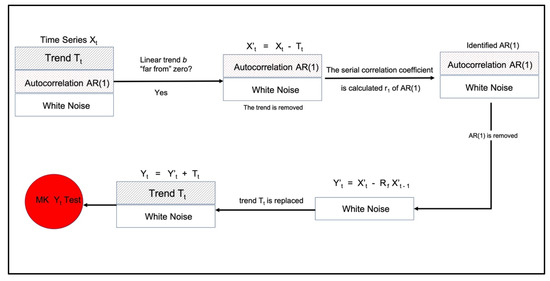
Figure 3.
Procedure proposed by [61] for the application of the Mann–Kendall test for trend detection in autoregressive (AR) time series (1).
In the present investigation, trend analysis was performed by applying the Mann–Kendall test after performing the procedures proposed by [61]. The tests were performed using the statistical software R.
3. Results
The first part of the procedures refers to the descriptive statistical analysis of the data. These procedures are relevant for a more consistent numerical analysis. Table 2 summarizes the values of the historical series for the maximum, average, and minimum air temperatures of each station.
Table 2.
Results of descriptive statistics of data from weather stations. (Temperature values in °C).
Two aspects of the data in Table 2 deserve particular attention. The coefficient of variation (CV) is a standardized measure of dispersion of a probability distribution or frequency distribution. It is often expressed as a percentage. The smaller the value, the more homogeneous the data will be, i.e., the less dispersion there will be around the mean.
According to [62], a CV is considered low, indicating a data set that is reasonably homogeneous when it is less than 30%. If this value is greater than 30%, the data set can be considered heterogeneous. A CV of 15% to 30% is considered medium, implying good precision. However, this standard varies according to the application.
In 87% of the sample data, the CV was less than 15%, indicating homogeneity. The CV values observed for minimum air temperatures stand out, which, in all the stations, remained greater than 10%. The values for FAL and CINDACTA remained in the medium range of data dispersion.
The second relevant indicator is skewness, which is a measure of the asymmetry of the distribution of a variable. If the skewness of S is zero, then the distribution represented by S is perfectly symmetric. If the skewness is negative, then the distribution is skewed to the left, while if the skew is positive, then the distribution is skewed to the right.
The values showed negative asymmetries for minimum and average air temperature and positive asymmetry for maximum air temperature at all stations. Although these values are asymmetrical, that is, with outlier trends, they are within the limits recommended by [63], which establishes, as outlier, a value greater than 1.5 dq. In general, all values lower than Li = Q1 − 1.5 dq or higher than Ls = Q3 + 1.5 dq are considered outliers.
Figure 4 shows monthly variations of minimum, average, and maximum air temperatures from 1980 to 2010 for each weather station, as well as the trend line of the data.
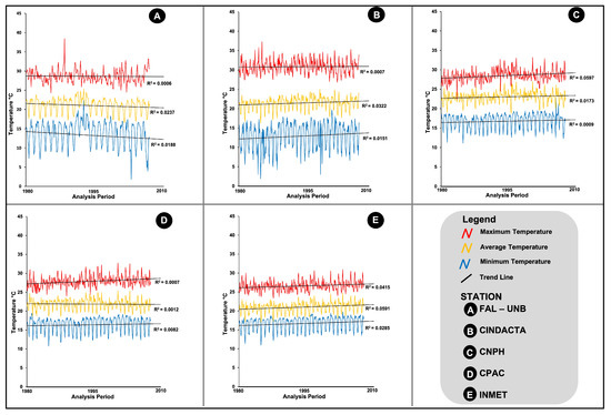
Figure 4.
Monthly variation of minimum, average, and maximum air temperatures, 1980–2010.
Figure 5 shows the boxplots for each weather station for the maximum, minimum, and average air temperatures. In descriptive statistics, a boxplot is a method for graphically depicting groups of numerical data through their quartiles. It is a standardized way of displaying the distribution of data based on a five-number summary (minimum value, first quartile (Q1), median, third quartile (Q3), and maximum value). It can tell you about the outliers and what their values are. It can also tell if the data are symmetrical, how tightly they are grouped, and if and how the data are skewed. The central position is given by the median, and dispersion is given by interquartile deviation dq = Q3 − Q2. The relative positions of Q1, Q2, and Q3 deal with the asymmetry of the distribution. The lengths of the tails of the distribution are given by the lines that go from the rectangle to the outliers.
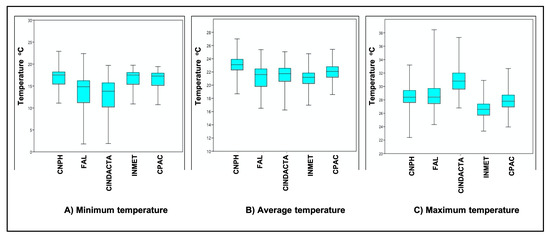
Figure 5.
Box plot graph for minimum, maximum, and average air temperatures at each weather station.
The graphs indicate that FAL and CINDACTA are the stations with the most discrepant records in comparison to the other weather stations, especially for minimum and maximum air temperatures. The steps taken so far have assessed the ability of the data to provide answers to support the application of statistical tests. The results show that the data are indeed suitable for the tests.
The results of the proposed statistical tests are presented below. Table 3 shows the p-values for each statistical test for each parameter analyzed per weather station. We chose to observe the variation of the p-value generated in each test, since the initial expectation was concentrated on identifying the existence or absence of a trend in the data series for Tmin, Tav, and Tmax. The criterion used to affirm whether the data shows a trend or not was the selection of measures that presented two or more p-value results within the significance level of p ≤ 0.05.
Table 3.
Test results (p-values) for the weather stations.
The Wald–Wolfwitz test found trends in all data series. According to the Cox–Stuart test, five measures showed no trend: three for Tmin, one for Tav, and one for Tmax. As for the Mann–Kendall test without adjustments, four measures did not show any trend: one for Tmin, one for Tav, and two for Tmax.
Following the previously defined criteria, among the 15 tests performed using these three methods, only two did not confirm a trend, namely, CPAC (Tav) and CINDACTA (Tmax); all the other measurements from the weather stations showed a tendency in air temperatures.
The results of the adjusted Mann–Kendall test (Table 3) show very different behavior from the previous results, with significant differences. By this test, trends were only identified in four of the data series: average air temperature at CNPH, and maximum air temperature at INMET, CPAC, and CNPH.
Based on the same criteria for determining trends in the data series, Table 4 indicates that there was a trend in air temperatures at all the stations studied. Notably, FAL is the only station where a decrease was identified.
Table 4.
Air temperature trends.
Considering the peculiarity of air temperature data collected in environments under the influence of urbanization and in humid/dry tropical climates, it is important for more than one statistical test to be used to study historical temperature trends. With its focus on assessing the complexity of this type of data and its temporal dynamics, this study showed that the Cox–Stuart and Mann–Kendall tests corroborated to validate the Wald–Wolfwitz test, contributing significantly to the general analysis of temperature trends in all seasons.
A 10 km radius from the location of the weather stations was set, which is within the range of suggested radiuses of influence used in similar studies (0.4 to 30 km) e.g., [64,65]. This radius demarcated a buffer zone covering 29 km2 for the analysis of changes in land use in the 1980–2010 period, with special attention to the growth of urban areas inside the buffer. Figure 6 shows the increase of urban areas around the weather stations between 1980 and 2010.
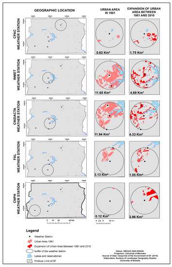
Figure 6.
Increase in urban area around the weather stations from 1980 to 2010.
Urbanization, the process of urban development, is characterized by the expansion of built-up areas. In the context of climate science, urbanization is usually regarded as a specific manifestation of land use change on a local scale. This process affects the local land surface, resulting in an altered surface climate in urban areas. The change in surface parameters induced by urbanization is a fundamental reason for the formation and evolution of urban climates and can interfere with data recording.
Between 1980 and 2010, there was a 105% increase in urban land use in the Federal District. It can be seen in Figure 6 that the urban area around all the weather stations grew in this period, albeit by different amounts. Table 5 shows the evolution of urban occupation around each weather station.
Table 5.
Evolution of urban occupation around each weather station.
4. Discussion
The combined analysis of the upward trends in air temperature and the increased urbanization in the areas of influence around the weather stations reveals a particularly notable situation at the CNPH and CPAC stations, where a higher rate of urbanization was associated with an upward trend in air temperature. Although an upward trend was also observed at the INMET and CINDACTA stations, the rate of increase was lower because they were already more urbanized in the first year of the time series and they are located in areas destined for urban expansion, resulting in effective occupation. At CNPH and CPAC, by contrast, the areas were originally intended for rural use, but over the years were occupied without due to urban planning and regulation.
The effects of urbanization on local climates and trends in climatic parameters have been studied by several researchers since it became noticeable that the intensity of urbanization renders significantly different climatic conditions in cities when compared to surrounding areas [65,66,67]. Cities change the climate, mainly on the local scale, through transformations in the land surface, generally resulting in increased temperatures and modified wind flows and relative humidity of the air [68].
Taking the results obtained here with those of [32], it can now be stated that there is an upward trend in air temperature in the Federal District. This statement is justified by the differences in methodologies and historical series used and the fact that the statistical robustness of this research is greater. The upward trends seen at most of the stations are most likely related to the influence of different land occupation patterns in the 1980–2010 period, an aspect that should be taken into account in urban planning.
To prove the existence of a relationship between urbanization and changes in air temperature in the Federal District, portable air temperature measuring instruments would have to be installed at different sites in the territory in order to analyze spatial variations in air temperature and identify the influence that the most built-up areas and the areas with higher density of vegetation have on air temperature variations during the year and under the predominance of different atmospheric systems.
5. Conclusions
This investigation was primarily concerned with assessing whether trend tests are capable of confirming or refuting the existence of trends in air temperature data in the Federal District of Brazil between 1980 and 2010. Five weather stations in the Federal District were selected and the maximum monthly temperature, average monthly temperature, and minimum monthly temperature data were analyzed.
The first three statistical tests (Table 3) revealed an upward trend for three stations and a downward trend for one station. For two stations, no trend was identified for average and maximum air temperature. Of the 15 data series analyzed, 67% pointed towards an increase in air temperature values, 13% were stable, and 20% pointed to a trend for reduced air temperatures.
The spatial distribution of the stations may be associated with issues that require further investigation, although some signs can be identified more easily. The INMET station, for example, is located in the center of the Federal District and has received the most anthropic pressure for urban use in recent years. The FAL station was the only one that showed downward trends from 1980 to 2010, which were validated in all the tests and for all measurements.
This research also confirmed that the Cox–Stuart and Mann–Kendall tests are reliable and useful in studies of temperature trends. The findings lead us to conclude that air temperature trends can be analyzed in two ways: the first using only the Wald–Wolfwitz test, which has shown compelling results, especially for studies that demand faster results; and the second option, combining it with the Cox–Stuart and Mann–Kendall tests for validation purposes, thereby yielding more robust and consistent results.
The analysis of the type of land use in the immediate surroundings of FAL revealed that it underwent the least anthropic transformation of the landscape of the five weather stations studied. If there is a persistent trend for increased air temperatures in the Federal District, this may negatively influence various sectors of society, particularly the health of the population, especially during the dry season when more cases of respiratory diseases are registered. These results could serve as an input for public administrators involved in public planning and policy-making.
Author Contributions
Conceptualization, V.A.S.; formal analysis, L.A.M.P.d.M., R.L.L., and E.T.S.; investigation, V.A.S., M.L.M., and E.T.S.; methodology, V.A.S. and R.R.d.F.; writing—original draft, E.T.S.; writing—proofreading and editing, R.L.L. All authors have read and agreed to the published version of the manuscript.
Funding
This research received no external funding.
Conflicts of Interest
The authors declare no conflict of interest.
References
- Jones, P.D.; Moberg, A. Hemispheric and large-scale surface air temperature variations: An extensive revision and an update to 2001. Boston J. Clim. 2003, 16, 206–223. [Google Scholar] [CrossRef]
- Stewart, I.D.; Oke, T.R. Methodological concerns surrounding the classification of urban and rural climate stations to define urban heat island magnitude. In Proceedings of the Sixth International Conference on Urban Climate, Goteborg, Sweeden, 12–16 July 2006; pp. 431–444. [Google Scholar]
- Shitara, H. Effects of buildings upon the winter temperature in Hiroshima city. Geogr. Rev. 1957, 30, 468–482. (In Japanese) [Google Scholar] [CrossRef][Green Version]
- Louw, W.J.; Meyer, J.A. Near-surface nocturnal winter temperatures in Pretoria. Notos 1965, 14, 49–65. [Google Scholar]
- Chandler, T.J. The Climate of London; Hutchinson: London, UK, 1965; p. 292. [Google Scholar]
- Ludwig, F.L. Urban Temperature Fields. Urban Climates; Technical Note n.108; WMO: Geneva, Switzerland, 1970; pp. 80–107. [Google Scholar]
- Sharon, D.; Koplowitz, R. Observations of the Heat Island of a Small Town; Meteorologische Rundschau: Stuttgart, Germany, 1972; Volume 25, pp. 143–146. [Google Scholar]
- Okoola, R.E. The Nairobi heat island.Kenya. J. Sci. Technol. 1980, 1A, 53–65. [Google Scholar]
- Oke, T.R. Boundary Layer Climates; Routledge: Abingdon on Thames, UK, 1987; p. 435. [Google Scholar]
- Robaa, S.M. Urban-suburban/rural differences over Greater Cairo, Egypt. Atmósfera 2003, 16, 157–171. [Google Scholar]
- Nunes da Silva, E.; Ribeiro, H. Temperature modifications in shantytown environments and thermal discomfort. Rev. Saúde Publica 2006, 40, 663–670. [Google Scholar]
- Amorim, M.C.C.T.; Dubreuil, V.; Cardoso, R.D.S. Modelagem espacial da ilha de calor urbana em presidente prudente (SP)—Brasil. Rev. Bras. Climatol. 2015, 11, 29–45. [Google Scholar] [CrossRef]
- Skarbit, N.; Stewart, I.D.; Unger, J.; Gál, T. Employing an urban meteorological network to monitor air temperature conditions in the ‘local climate zones’ of Szeged, Hungary. Int. J. Climatol. 2017, 37 (Suppl. S1), 582–596. [Google Scholar] [CrossRef]
- Amorim, M.C.C.T. Intensidade e forma da ilha de calor urbana em Presidente Prudente/SP. Geosul (UFSC) 2005, 20, 65–82. [Google Scholar]
- Amorim, M.C.C.T. Climatologia e gestão do espaço urbano. Mercator (Fortaleza. Online) 2010, 9, 71–90. [Google Scholar]
- Mendonça, F.; Dubreuil, V. L’étude du climat urbain au Brésil: Etat actuel et contribution de la télédétection. In Environnement et Télédétection au Brésil; Presses Universitaires de Rennes: Rennes, France, 2002; pp. 135–146. [Google Scholar]
- Amorim, M.C.C.T.; Dubreuil, V.; Quenol, H.; Sant’anna, J.L. Características das ilhas de calor em cidades de porte médio: Exemplos de Presidente Prudente (Brasil) e Rennes (França). Confins [Online] 2009, 7, 16. [Google Scholar] [CrossRef]
- Amorim, M.C.C.T. O Clima Urbano de Presidente Prudente/SP. São Paulo. Ph.D. Thesis, Faculty of Philosophy, Letters and Human Sciences, University of Sao Paulo, Sao Paulo, Brazil, 2000. [Google Scholar]
- Stewart, I.D.; Oke, T.R. Newly developed “thermal climate zones” for defining and measuring urban heat island magnitude in the canopy layer. In Proceedings of the Preprints, T.R. Oke Symposium & Eighth Symposium on Urban Environment, Phoenix, AZ, USA, 10 January 2009; pp. 11–15. [Google Scholar]
- Oke, T.R. Initial Guidance to Obtain Representative Meteorological Observations at Urban Sites; IOM Report 81, WMO/TD. No. 1250; World Meteorological Organization: Geneva, Switzerland, 2006; Available online: http://www.wmo.int/pages/prog/www/IMOP/publications/IOM-81/-UrbanMetObs.pdf (accessed on 15 July 2020).
- Hansen, J.; Lebedeff, S. Global trends of measured surface air temperature. J. Geophys. Res. 1987, 92, 13345–13372. [Google Scholar] [CrossRef]
- Back, A.J. Aplicação de análise estatística para identificação de tendências climáticas. Pesq. Agropec. Bras. 2001, 36, 717–726. [Google Scholar] [CrossRef]
- Munuzzi, R.B.; Caramori, P.H. Tendência climática sazonal e anual da quantidade de chuva no estado do Paraná. Rev. Bras. Meteorol. 2010, 25, 237–246. [Google Scholar]
- Silva, H.J.F. Análise de Tendência e Caracterização Sazonal e Interanual da Evapotranspiração de Referência Para o Sudoeste da Amazônia Brasileira: Acre, Brasil. Master’s Thesis, Federal University of Rio Grande do Norte, Natal, Brazil, 2010. [Google Scholar]
- Dos Santos Gomes, A.C.; da Silva Costa, M.; Coutinho, M.D.L.; do Vale, R.S.; dos Santos, M.S.; da Silva, J.T.; Fitzjarrald, D.R. Análise estatística das tendências de elevação nas séries de temperatura média máxima na amazônia central: Estudo de caso para a região do oeste do Pará. Rev. Bras. Climatol. 2015, 11, 17. [Google Scholar]
- Chattopadhyay, S.; Edwards, D.R. Long-term trend analysis of precipitation and air temperature for Kentucky, United States. Climate 2016, 4, 10. [Google Scholar] [CrossRef]
- Ray, L.K.; Goel, N.K.; Arora, M. Trend analysis and change point detection of temperature over parts of India. Theor. Appl. Climatol. 2019, 138, 153–167. [Google Scholar] [CrossRef]
- Livada, I.; Synnefa, A.; Haddad, S.; Paolini, R.; Garshasbi, S.; Ulpiani, G.; Fiorito, F.; Vassilakopoulou, K.; Osmond, P.; Santamouris, M. Time series analysis of ambient air-temperature during the period 1970–2016 over Sydney, Australia. Sci. Total Environ. 2019, 648, 1627–1638. [Google Scholar] [CrossRef]
- Higashino, M.; Stefan, H.G. Trends and correlations in recent air temperature and precipitation observations across Japan (1906–2005). Theor. Appl. Climatol. 2020, 140, 517–531. [Google Scholar] [CrossRef]
- Ribeiro, M.d.S.B. Variação Climática no Distrito Federal: Componentes e Perspectivas Para o Planejamento Urbano. Master’s Thesis, Faculty of Arquitecture and Urbanism, University of Brasilia, Brasilia, Brasil, 2000. [Google Scholar]
- De Mello Baptista, G.M. Estudo multitemporal do fenômeno ilhas de calor no Distrito Federal. Medio Ambient. 2002, 2, 3–17. [Google Scholar]
- Steinke, E.T.; de Andrade Souza, G.; Saito, C.H. Análise da variabiliade da temperatura do ar e da precipitação no Distrito Federal no período de 1965/2003 e sua relação com uma possível alteração climática. Rev. Bras. Climatol. 2005, 1, 131–145. [Google Scholar]
- Codeplan. Atlas do Distrito Federal; Codeplan: Brasilia, Brazil, 1984; Volume II. [Google Scholar]
- Semarh. Mapa Ambiental do Distrito Federal; Semarh: Brasília, Brazil, 2000; Scale: 1:100.000. CD-ROM.
- Steinke, V.A. Uso Integrado de Dados Digitais Morfométricos (Altimetria e Sistema de Drenagem) na Definição de Unidades Geomorfológicas no Distrito Federal, Brasília. Master’s Thesis, University of Brasilia, Brasilia, Brazil, 2003. 101 f. [Google Scholar]
- Steinke, V.A.; Sano, E.E. Semi-automatic identification, gis-based morphometry of geomorphic features of federal district of brazil. Rev. Bras. Geomorfol. 2011, 12, 3–9. [Google Scholar] [CrossRef]
- Barros, J.R. A chuva no Distrito Federal: O Regime e as Excepcionalidades do Ritmo. Master’s Thesis, State Paulista University, Rio Claro, Brazil, 2003. 221 f. [Google Scholar]
- Barros, J.R.; Zavattini, J.A.; Pitton, S. Doenças respiratórias e tipos de tempo no Distrito Federal. In Saberes e Fazeres Geográficos; Gerardi, L.H.O., Ferreira, E.R., Eds.; UNESP/IGCE e AGETEO: Rio Claro, Brazil, 2008; Volume 1, pp. 9–23. [Google Scholar]
- Steinke, E.T. Considerações Sobre Variabilidade e Mudança Climática no Distrito Federal, suas Repercussões nos Recursos Hídricos e Informação ao Grande Público. Ph.D. Thesis, University of Brasilia, Brasilia, Brazil, 2004. 201 f. [Google Scholar]
- Morettin, P.A.; Toloi, C.M.C. Análise de Séries Temporais, 2nd ed.; E. Blucher: Sao Paulo, Brazil, 2006. [Google Scholar]
- Neves, A.I.L.R.N.C.N. Detecção de Tendências no Padrão Temporal de Variáveis Hidrológicas. Aplicação à Precipitação a Diferentes Escalas Temporais. Covilhã. Master’s Thesis, University of Beira Interior, Covilha, Portugal, 2012. 192 f. [Google Scholar]
- Sonali, P.; Nagesh, K.D. Review of trend detection methods and their application to detect temperature changes in India. J. Hydrol. 2013, 476, 212–227. [Google Scholar] [CrossRef]
- Horos, M.T.; Dalfes, N.; Karaca, M.; Yenigün, O. A comparative assessment of different methods for detecting inhomogeneities in Turkish temperature data set. Int. J. Climatol. 1998, 18, 561–578. [Google Scholar] [CrossRef]
- Tröger, F.H.; Pante, A.R. Análise de estacionariedade em séries de vazões naturais médias anuais de estações da bacia do rio Tapajós. In Proceedings of the Simpósio Brasileiro De Recursos Hídricos, Campo Grande, Brazil, 22–26 November 2009; Anais Campo Grande: ABRH, 2009. Available online: https://www.abrhidro.org.br/SGCv3/publicacao.php?PUB=3&ID=110&SUMARIO=1792 (accessed on 15 July 2020).
- Coelho, M.; Fernandes, C.; Scapulatempo, V.; Detzel, D.H.M.; Mannich, M. Statistical validity of water quality time series in urban watersheds. RBRH 2017, 22, e51. [Google Scholar] [CrossRef]
- Rao, A.R.; Humed, K.H. Frequency analysis of Upper Cauvery flood data by L-moments. Water Resour. Manag. 1994, 8, 83–201. [Google Scholar] [CrossRef]
- Rao, A.R.; Humed, K.H. Flood Frequency Analysis; CRC Press: Boca Raton, FL, USA, 2000. [Google Scholar]
- Cox, D.R.; Stuart, A. Some Quick Tests for Trend in Location and Dispersion; Biometrika: London, UK, 1965; Volume 42, pp. 80–95. [Google Scholar]
- Morettin, P.A.; Toloi, C.M.C. Modelos de Função de Transferência; ABE: Sao Paulo, Brazil, 1989.
- McCuen, R.H. Modeling Hydrologic Change: Statistical Methods; Lewis Publishers: Boca Raton, FL, USA; London, UK; New York, NY, USA; Washington, DC, USA, 2003. [Google Scholar]
- Niedzielski, T.; Kosek, W. A required data span to detect sea level rise. In Advances in Marine Navigation and Safety of Sea Transportation; Weintrit, A., Ed.; Gdynia Maritime University: Gdynia, Poland, 2007; pp. 367–371. [Google Scholar]
- Mann, H.B. Non-parametric test against trend. Econometrica 1945, 13, 245–259. [Google Scholar] [CrossRef]
- Kendall, M.G. Rank Correlation Methods, 4th ed.; Charles Griffin: London, UK, 1975. [Google Scholar]
- Gilbert, R.O. Statistical Methods for Environmental Pollution Monitoring; Van Nostrand Reinhold: New York, NY, USA, 1987. [Google Scholar]
- Partal, T.; Kahya, E. Trend analysis in Turkish precipitation data. Hydrol. Process 2006, 20, 2011–2026. [Google Scholar] [CrossRef]
- Jaagus, J. Climatic changes in Estonia during the second half of the 20th century in relationship with changes in large-scale atmospheric circulation. Theor. Appl. Climatol. 2006, 83, 77–88. [Google Scholar] [CrossRef]
- Modarres, R.; da Silva, V.P.R. Rainfall trends in arid and semi-arid regions of Iran. J. Arid. Environ. 2007, 70, 344–355. [Google Scholar] [CrossRef]
- Tabari, H.; Marofi, S.; Ahmadi, M. Long-term variations of water quality parameters in the Maroon River, Iran. Environ. Monitor. Assess. 2010, 177, 273–287. [Google Scholar] [CrossRef] [PubMed]
- Tabari, H.; Marofi, S.; Hosseinzadeh Talaee, P.; Mohammadi, K. Trend analysis of reference evapotranspiration in the western half of Iran. Agric. For. Meteorol. 2011, 151, 128–136. [Google Scholar] [CrossRef]
- Yue, S.; Pilon, P.; Phinney, B.; Cavadias, G. The influence of autocorrelation on the ability to detect trend in hydrological series. Hydrol. Process. 2002, 16, 1807–1829. [Google Scholar] [CrossRef]
- Gomes, F.P. Curso de Estatística Experimental, 15th ed.; Esalq. SP: Piracicaba, Brazil, 2009. [Google Scholar]
- Triola, M. Minitab Student Laboratory Manual and Workbook, 10th ed.; Addison-Wesley: Boston, MA, USA, 2006. [Google Scholar]
- World Meteorological Organization (WMO). Guide to Meteorological Instruments and Methods of Observation WMO-No. 8; WMO: Geneva, Switzerland, 2018; Available online: https://library.wmo.int/index.php?lvl=notice_display&id=12407#.XvesWGT0n6Y (accessed on 15 July 2020).
- Peña Quiñones, A.J.; Chaves Cordoba, B.; Salazar Gutierrez, M.R.; Keller, M.; Hoogenboom, G. Radius of influence of air temperature from automated weather stations installed in complex terrain. Theor. Appl. Climatol. 2019, 137, 1957–1973. [Google Scholar] [CrossRef]
- Landsberg, H.E. The Urban Climate; Academic: Orlando, FL, USA, 1981; p. 275. [Google Scholar]
- Gartland, L. Ilhas de Calor: Como Mitigar Zonas de Calor em Áreas Urbanas; Translated by Silvia Helena Gonçalves; Oficina de Textos: Sao Paulo, Brazil, 2010. [Google Scholar]
- Ruth, M.; Baklanov, A. Urban climate science, planning, policy and investment challenges. Urban Clim. 2012, 1, 1–3. [Google Scholar] [CrossRef]
- De Figueiredo Monteiro, C.A. Teoria e Clima Urbano; IGEO/USP: Sao Paulo, Brazil, 1976. [Google Scholar]


© 2020 by the authors. Licensee MDPI, Basel, Switzerland. This article is an open access article distributed under the terms and conditions of the Creative Commons Attribution (CC BY) license (http://creativecommons.org/licenses/by/4.0/).