Future Scenarios of Soil Erosion in the Alps under Climate Change and Land Cover Transformations Simulated with Automatic Machine Learning

 ,
,  ,
,  and
and
Abstract
1. Introduction
2. Materials
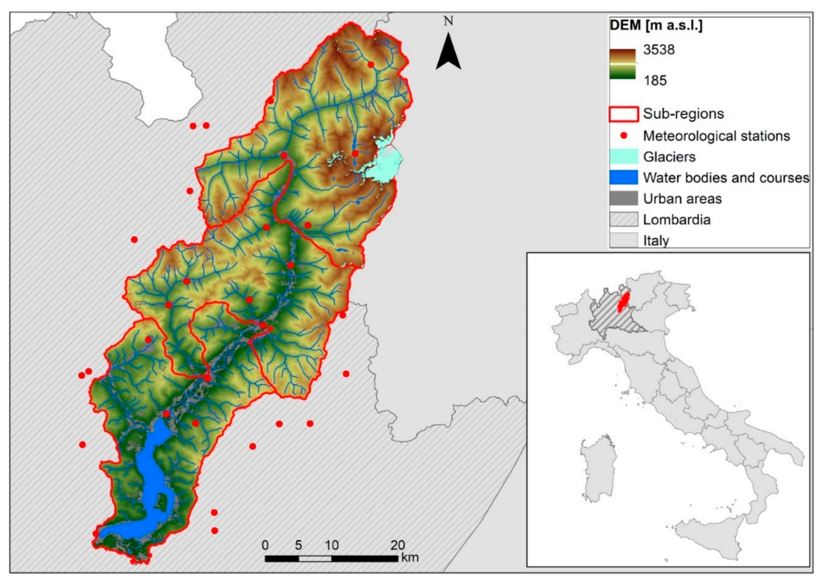
2.1. Study Area
2.2. Data
- Raster Digital Elevation Model (DEM) of Regione Lombardia with 30-meters spatial resolution (Figure 1). We used the DEM for estimating the topographic factor (i.e., LS-factor), for the interpolation of the meteorological data and for climate simulations;
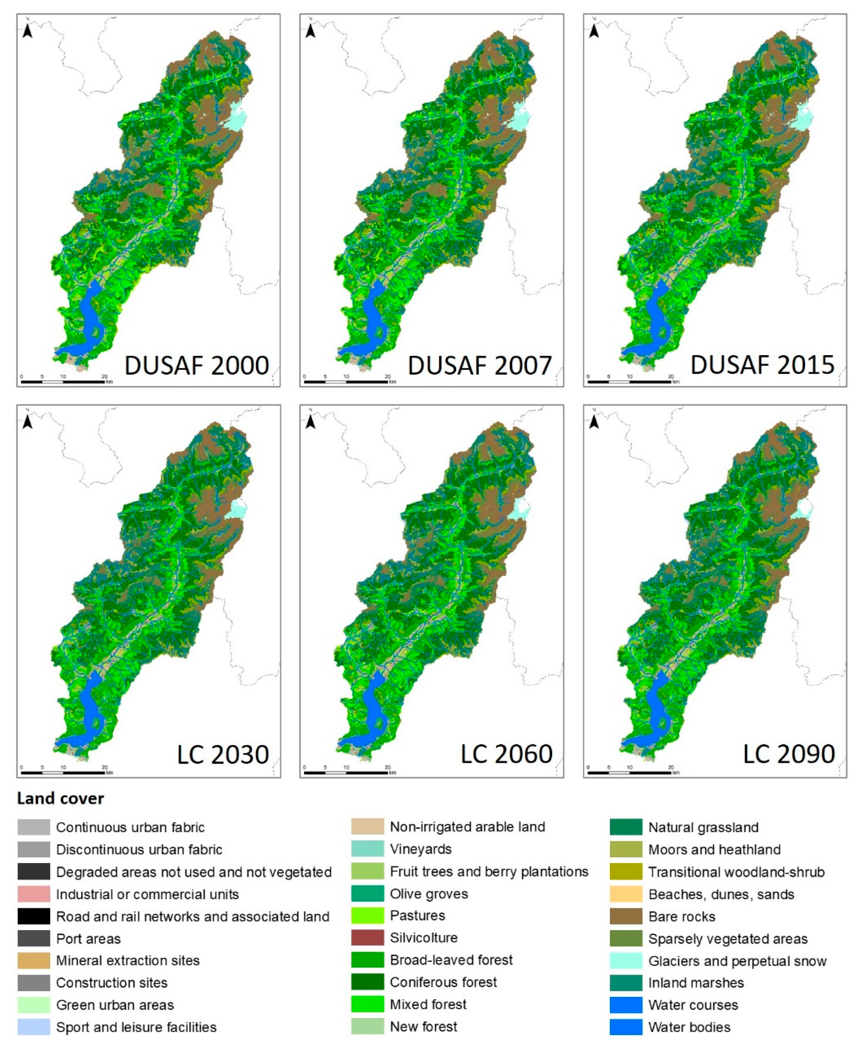
- Vector Destinazione d’Uso dei Suoli Agricoli e Forestali (DUSAF) of Regione Lombardia. DUSAF are land cover maps organized in five hierarchical levels, where the first three levels are compliant with the European Corine Land Cover. We used the DUSAF maps of 2000, 2007, and 2015 for the estimation of the vegetation sheltering factor (i.e., C-factor) and for the simulation of future land cover;
- Vector soil map of Regione Lombardia. We used this map for the evaluation of the soil erodibility (i.e., K-factor) [35];
- Vector maps of terracing provided by Adamello Park authorities. We used this information for simulating the impact of agricultural protection practices on soil erosion (i.e., P-factor);
- Hourly time series of precipitation and air temperature (period 2003–2017) recorded by 30 rain gauges and 28 thermometers of the Environmental Protection Agency of Regione Lombardia (Figure 1). We used these data to provide the estimates of observed rainfall erosivity (i.e., R-factor) and to calibrate the parameters of the statistical spatio-temporal downscaling used for climate simulations.
3. Methods
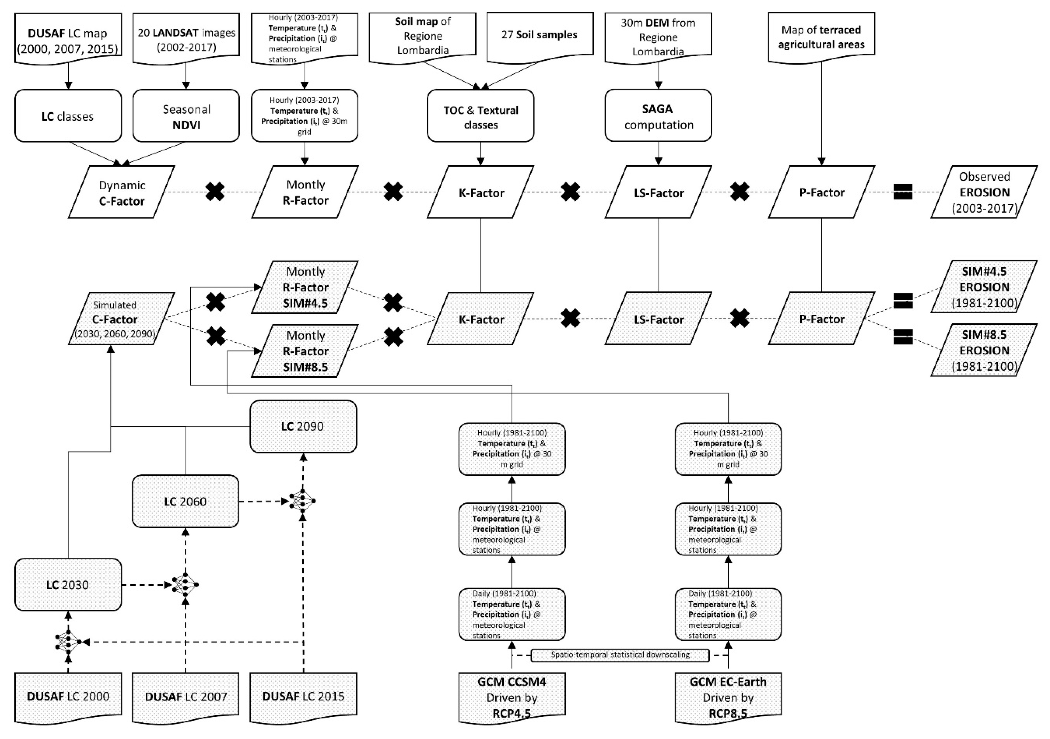
3.1. The D-RUSLE Erosion Model
- R (called R-factor) is the rainfall erosivity factor [MJ mm ha−1 h−1 yr−1]. This parameter describes the meteorological forcing to erosion and is function of precipitation rate, air temperature, and snow cover dynamics;
- C (called C-factor) is the cover management factor [-]. This parameter describes the sheltering effect of land cover (mainly vegetation) toward soil erosion. Lower C-factor values correspond to higher protection, thus lower erosion;
- K (called K-factor) is the soil erodibility factor [t ha h ha−1 MJ−1 mm−1]. This parameter describes the soil structure and organic matter content, which can influence its natural inclination to erosion;
- LS (called LS-factor) is the topographic characteristics of the area [-]. This parameter describes the impact of slope length and slope steepness on soil erosion;
- P (called P-factor) is the support practice factor [-]. This parameter describes the effectiveness of anti-erosive practices adopted for land management, if any.
3.2. Climate Scenarios
- RCP2.6: peak in radiative forcing at 3 [W m−2] (490 ppm CO2 equivalent at 2040), and subsequent decline to 2.6 [W m−2]);
- RCP4.5: stabilization to 4.5 [W m−2] (650 ppm CO2 equivalent at 2070);
- RCP8.5: radiative forcing up to 8.5 [W m−2] (1370 ppm CO2 equivalent by 2100).
3.3. Projections of Precipitation, Temperature, and Rainfall Erosivity
- [mm h−1] is the effective hourly intensity of precipitation;
- is the monthly number of hours.
- [mm h−1] is the precipitation intensity (rain + snow);
- [mm] is the snow water equivalent;
- [°C] is the air temperature;
- [°C] is the threshold temperature below which all the precipitation is snow ( −3 °C);
- [°C] is the threshold temperature above which the precipitation is rain ( 0 °C);
- [°C] is the threshold temperature above which snow melting begins (°C);
- [mm h−1 °C−1] is the snow melting rate ( 0.18 [mm h−1 °C−1]).
3.4. Land Cover Scenarios
3.5. Projections of Future Cover Management Factor
- 1981–2010 (reference period): DUSAF 2000 map;
- 2011–2040: simulated LC 2030 map;
- 2041–2070: simulated LC 2060 map;
- 2071–2100: simulated LC 2090 map.
4. Results
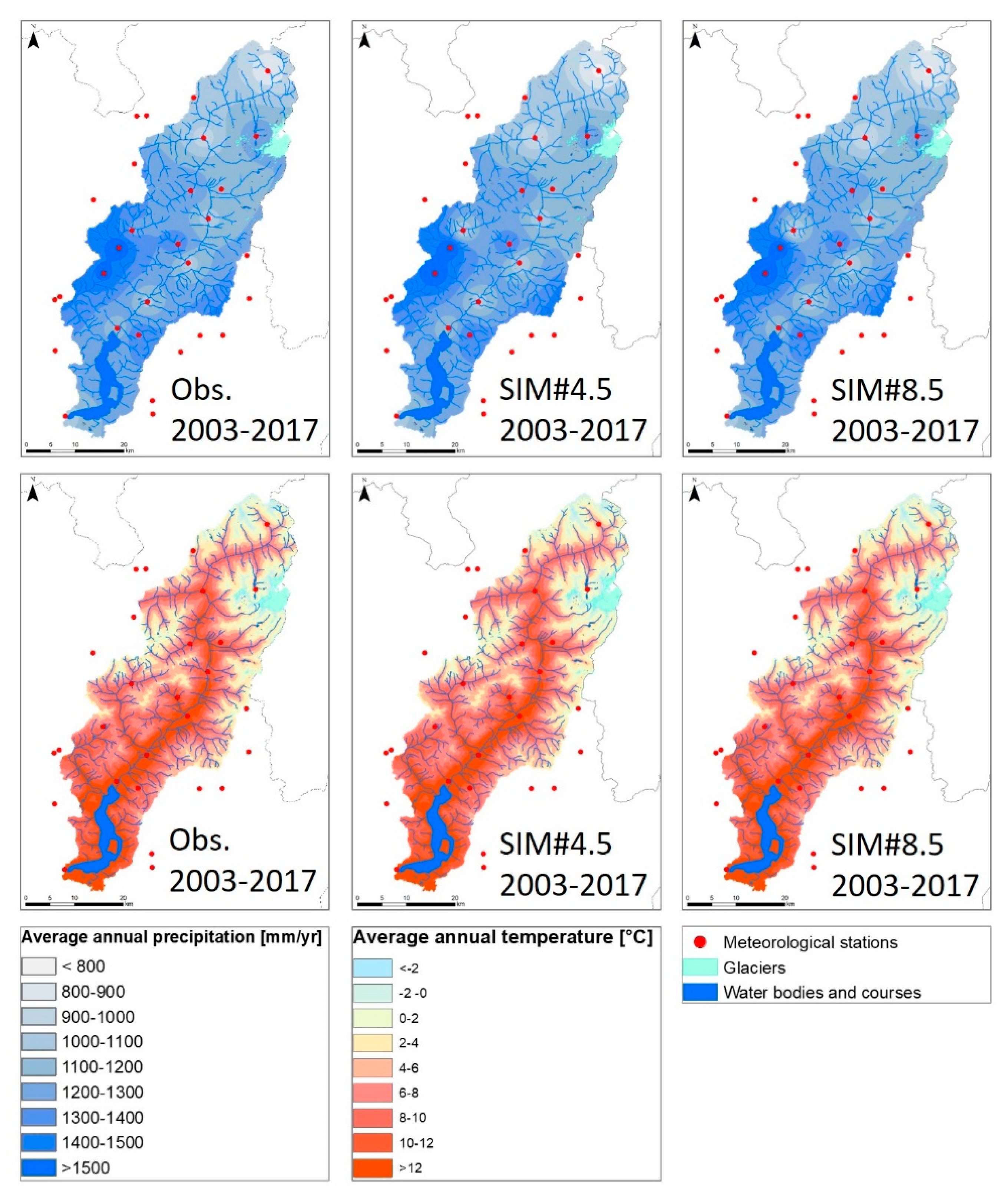
4.1. Projections of Precipitation, Temperature, and Rainfall Erosivity
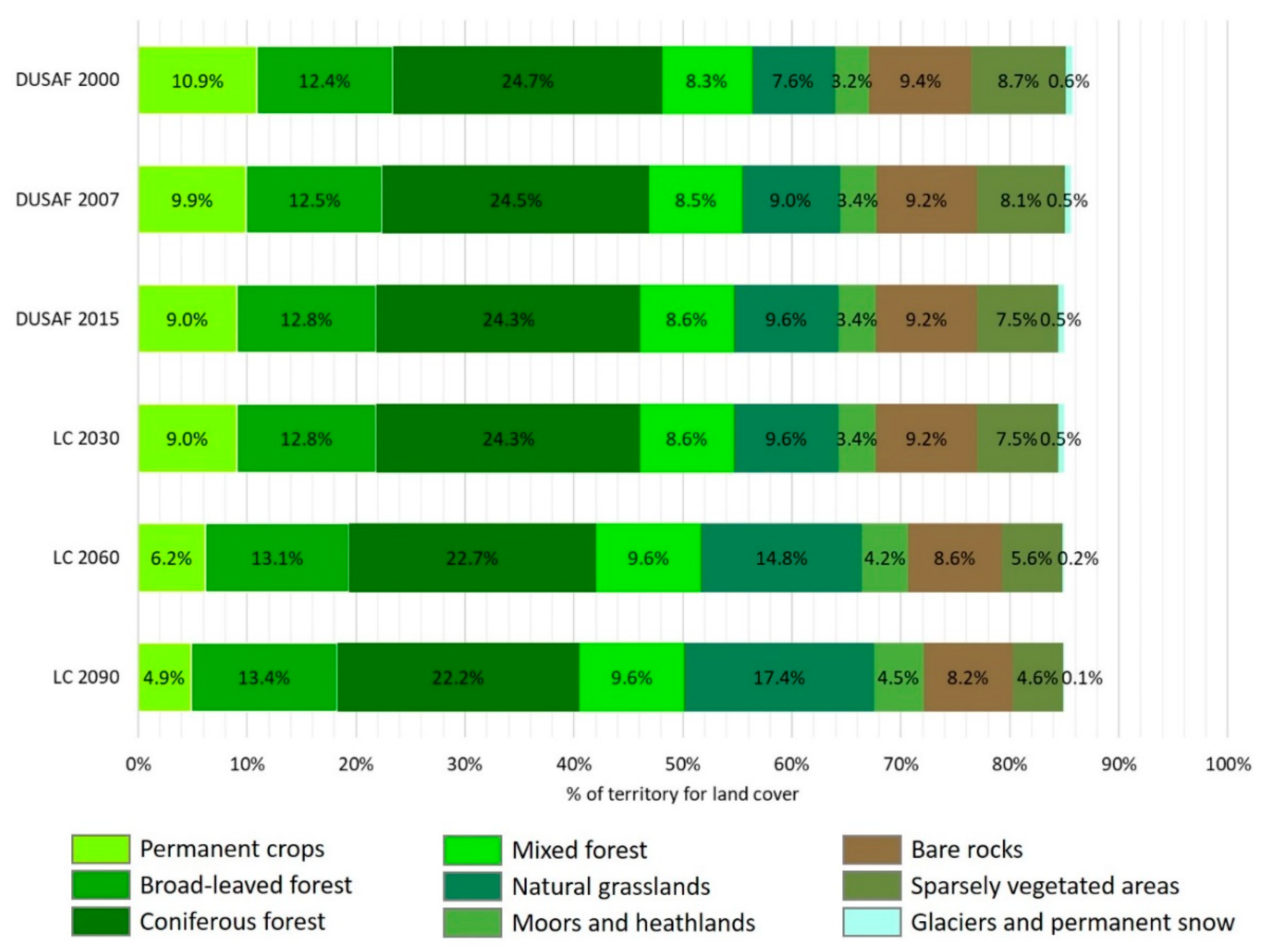
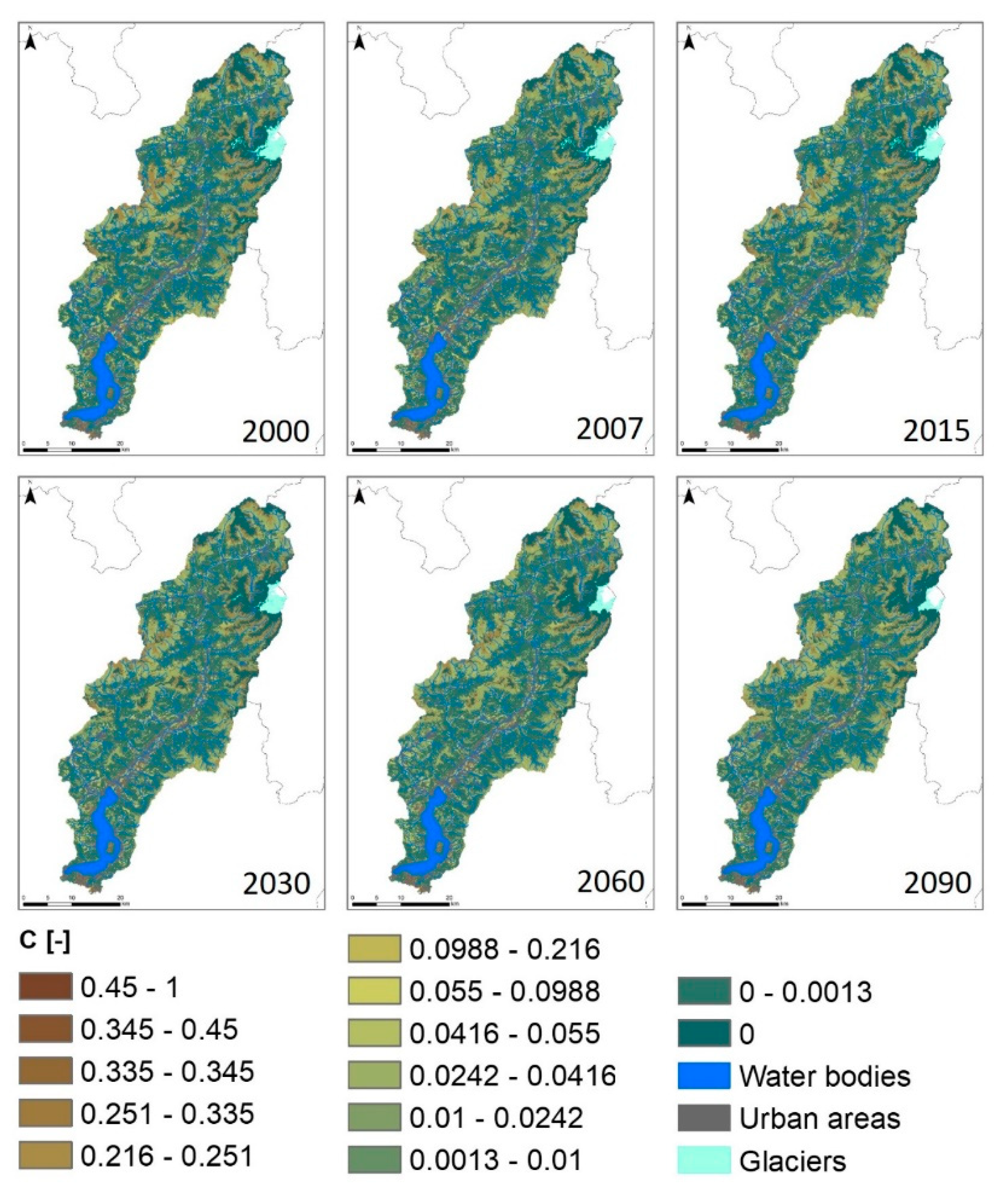
4.2. Projections of Future Land Cover and Cover Management Factor
- Sparsely vegetated areas and pastures continue to reduce almost constantly until 2090;
- Natural grasslands continue to increase almost constantly until 2090;
- Moors and heathlands show a rapid increase until 2060 and then a slower increase until 2090;
- Transitional woodland-shrubs and bare rocks show respectively a minimal increase and a minimal decrease in the simulation periods;
- Glacier and perpetual snow considerably reduce (from −37% in the first 30-years period to
- −52% in the third 30-years period), in accordance with the expected retreat of the Adamello glacier and the disappearance of the Ortles glacier.
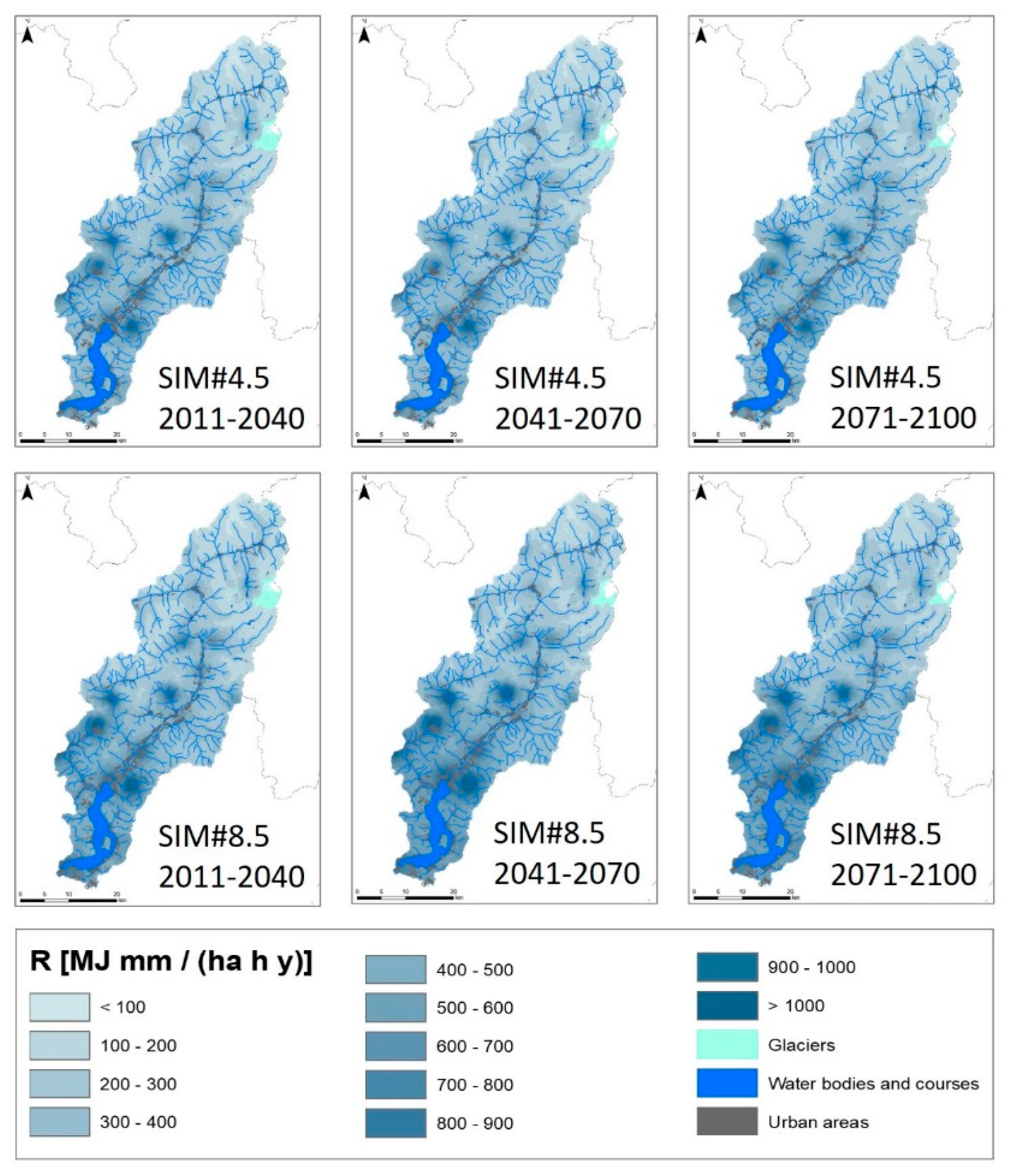
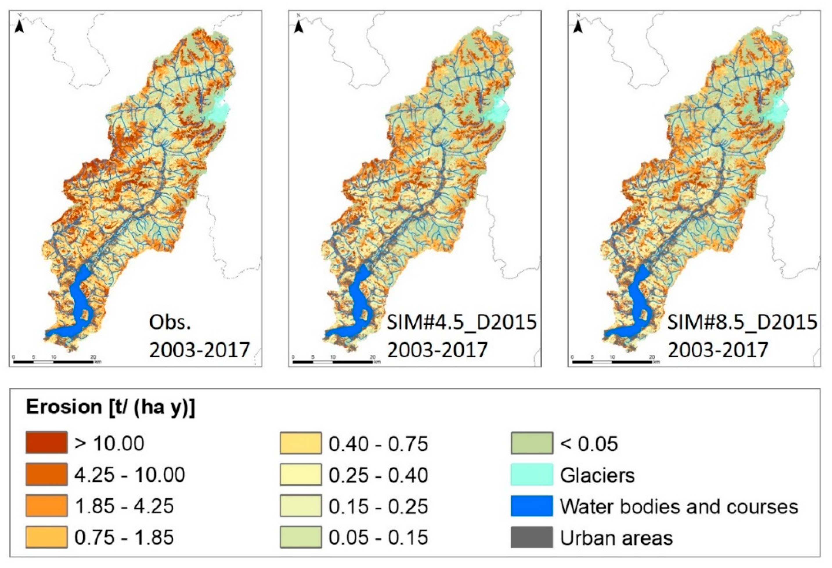
4.3. Effect of Climate Projections on the Estimates of Soil Erosion
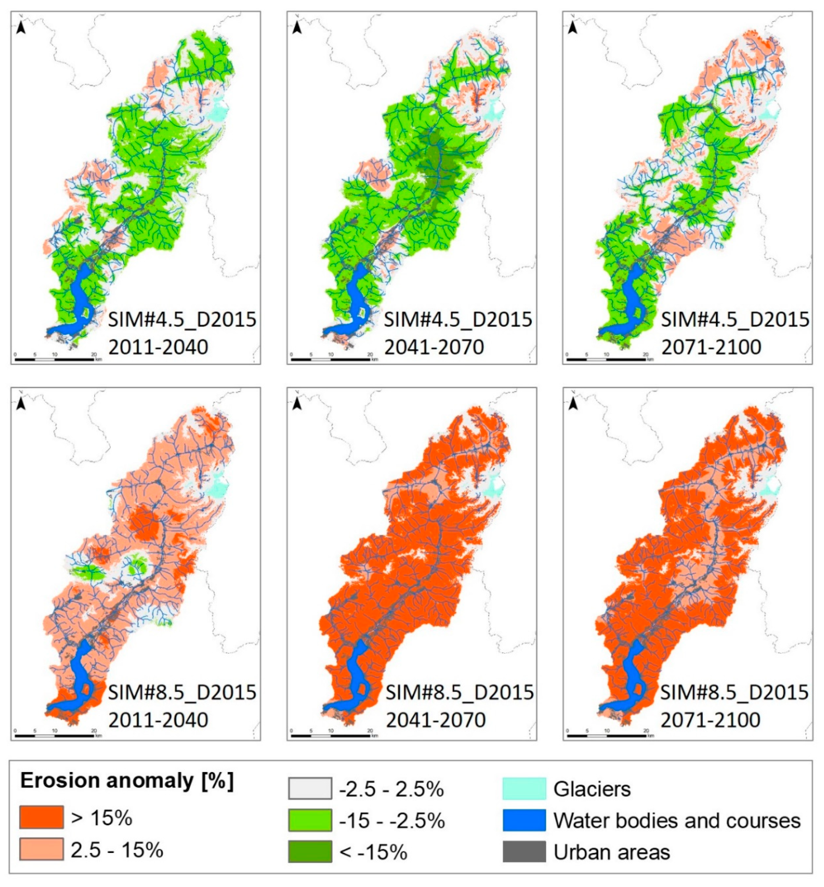
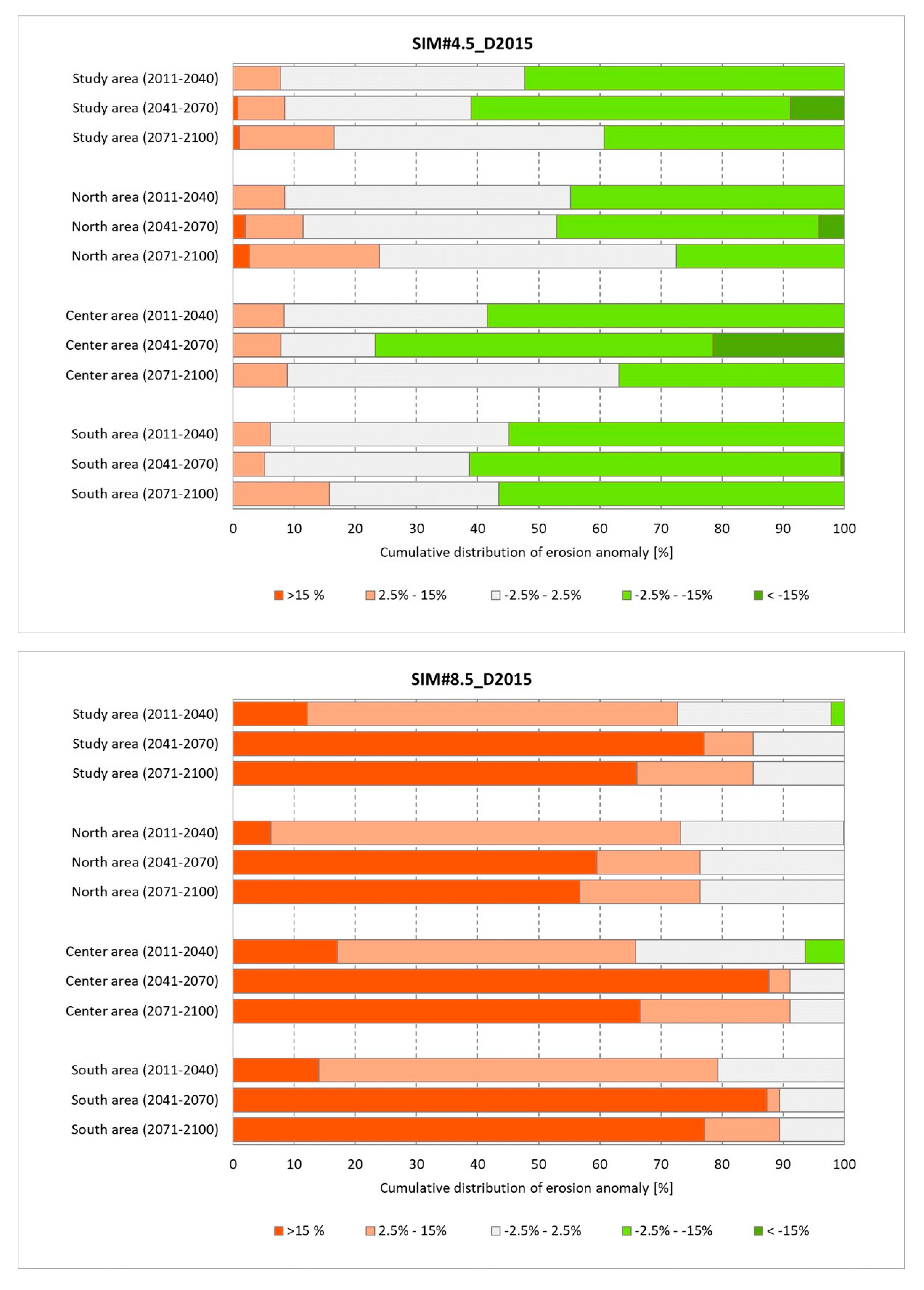
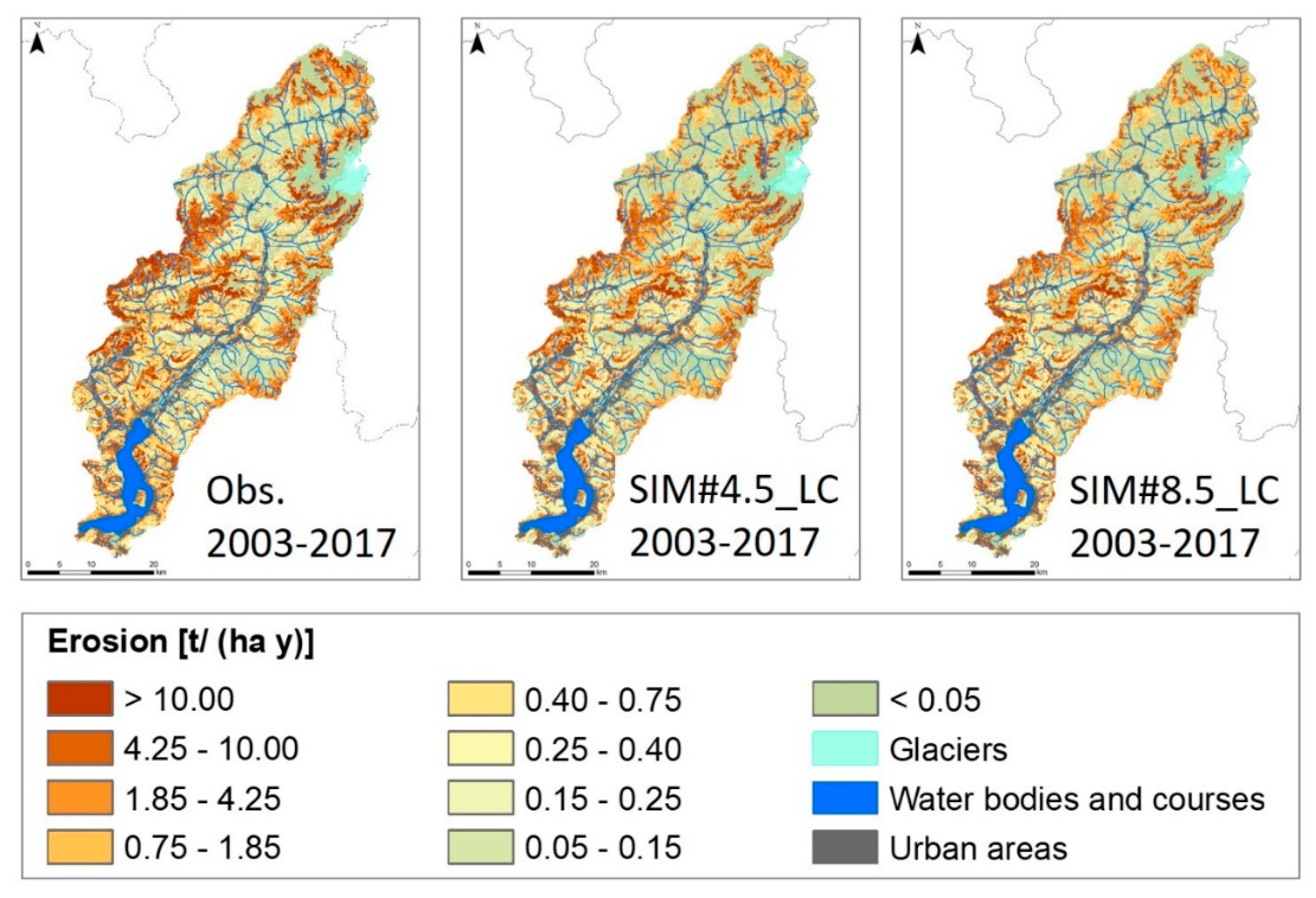
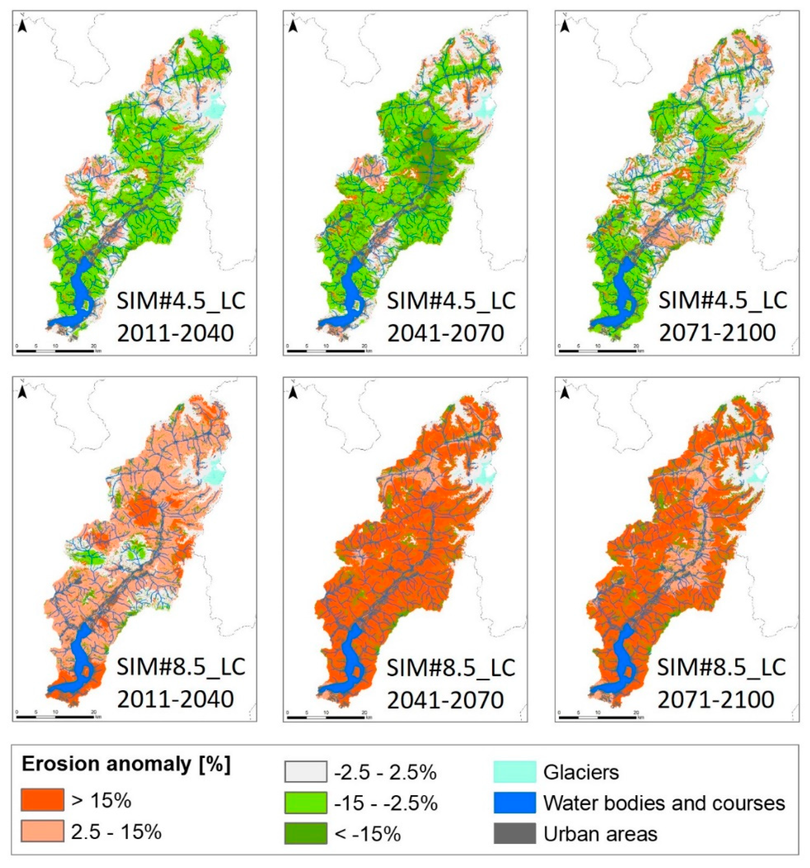
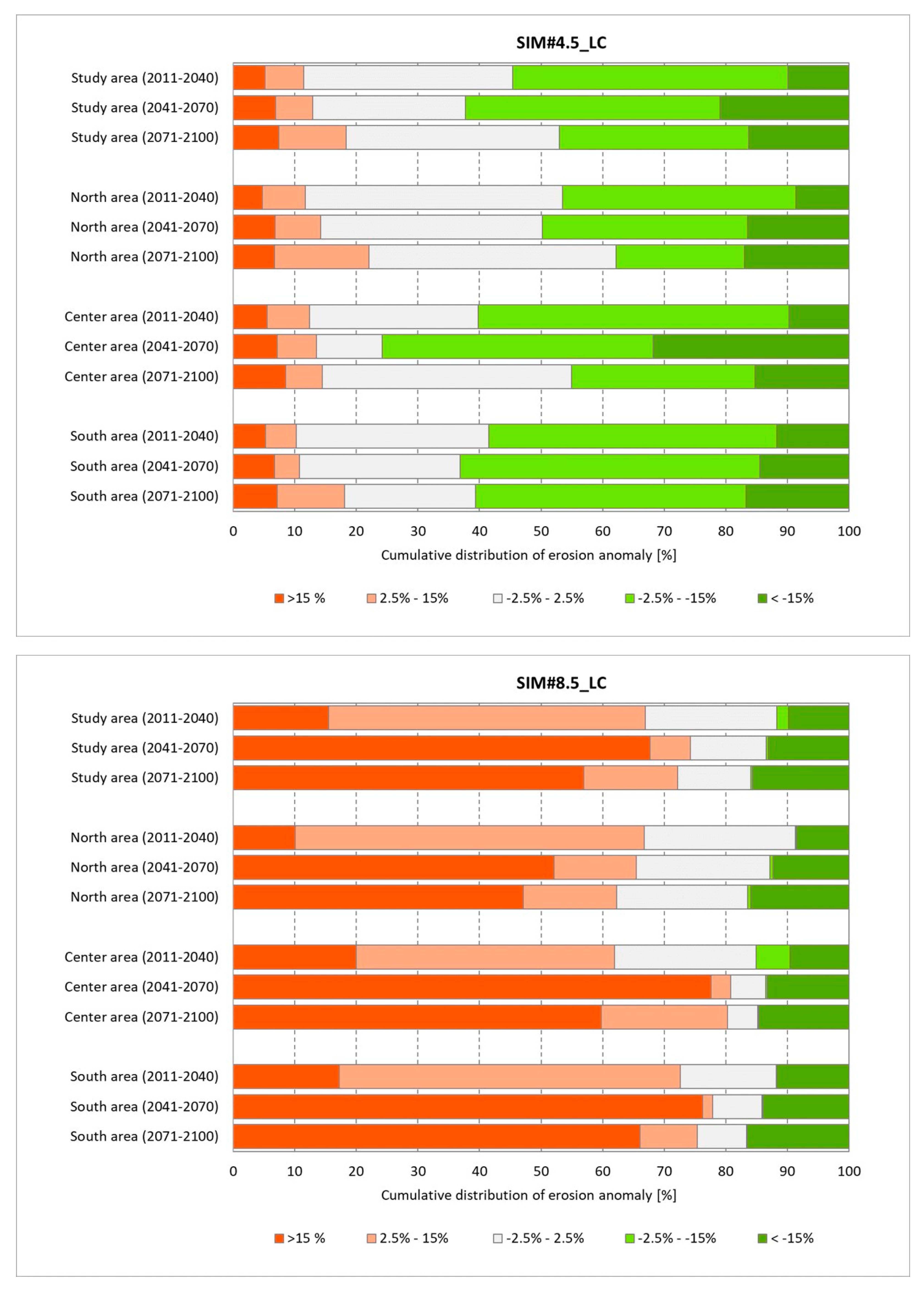
4.4. Combined Effects of Climate and Land Cover Projections on the Estimates of Soil Erosion
5. Discussion
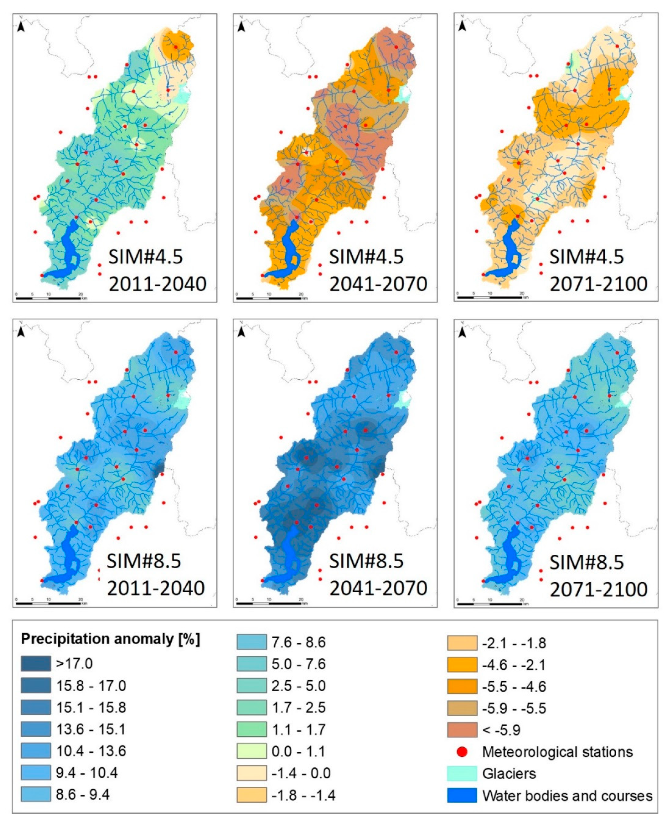
5.1. Projections of Precipitation
- North: 5.5% of this territory will have a slight increase, 9.0% will have a slight decrease and the rest will have almost constant precipitation;
- Center: 19% of this territory will have a slight increase and the rest will have almost constant precipitation;
- South: 25% of this territory will have a slight increase and the rest will have almost constant precipitation.
5.2. Projections of Temperature
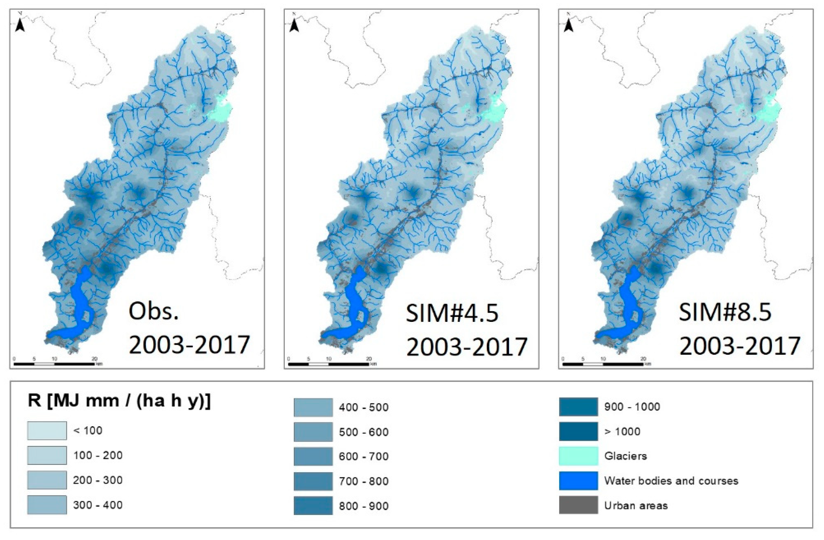
5.3. Simulation of Rainfall Erosivity
- North: the bias is +5% for SIM#4.5 and −33% for SIM#8.5;
- Center: the bias is −29% for both SIM#4.5 and SIM#8.5;
- South: the bias is −23% for SIM#4.5 and −17% for SIM#8.5.
5.4. Projections of Future Land Cover and Cover Management Factor
- “Sparsely vegetated areas” cover 8.7% of the study area in 2000 (it is the third more frequent land cover) but are projected to reduce to 4.6% in 2090;
- “Pastures” cover 10.9% of the study area in 2000 (it is the fifth more frequent land cover) but are projected to reduce to 4.9% in 2090;
- “Non-irrigated arable land” covers 1.1% of the study area in 2000 but is projected to reduce to 0.7% in 2090.
- is the skill score for the sub-model i;
- is the measured accuracy of the transition/persistence for class j for the sub-model i;
- is the expected accuracy of the transition/persistence for class j for the sub-model i;
- is the percentage of land cover class j for the sub-model i;
- is the number of transitions in the sub-model i;
- is the number of persistence classes in the sub-model i.
5.5. Estimates of Future Soil Erosion
5.6. Comparison to Similar Studies
- Working scale. The majority of papers performs global, national, or regional analysis, and not local-scale analysis;
- Topographic and land cover characteristics of the study areas;
- Model used to estimate soil erosion;
- Model used to project climate and land cover changes.
5.7. Current Limitations
6. Conclusions
Author Contributions
Funding
Acknowledgments
Conflicts of Interest
References
- Panagos, P.; Borrelli, P.; Poesen, J.; Ballabio, C.; Lugato, E.; Meusburger, K.; Montanarella, L.; Alewell, C. The new assessment of soil loss by water erosion in Europe. Environ. Sci. Policy 2015, 54, 438–447. [Google Scholar] [CrossRef]
- European Commission (EC). Communication from the Commission to the Council, the European Parliament, the European Economic and Social Committee and Committee of the Regions “Thematic Strategy for Soil Protection” (COM((2006)231). Available online: http://eur-lex.europa.eu/legal-content/EN/TXT/?uri=CELEX:52006DC0231 (accessed on 6 February 2020).
- Derpsch, R. Understanding the Process of Soil Erosion and Water Infiltration. FAO Publication. 1991. Available online: http://www.fao.org/tempref/agl/emailconf/soilmoisture/t1_Derpsch_1.doc (accessed on 6 February 2020).
- Boardman, J.; Poesen, J. Soil Erosion in Europe; John Wiley and Sons: Chichester, UK, 2007. [Google Scholar]
- Chapman, D.V. Water Quality Assessments: A Guide to the Use of Biota, Sediments and Water in Environmental Monitoring, 2nd ed.; Taylor & Francis: Milton Park, UK; Abingdon-on-Thames, UK; Oxfordshire, UK, 2006. [Google Scholar]
- Bay, S.M.; Zeng, E.Y.; Lorenson, T.D.; Tran, K.; Alexander, C. Temporal and spatial distributions of contaminants in sediments of Santa Monica Bay, California. Mar. Environ. Res. 2003, 56, 255–276. [Google Scholar] [CrossRef]
- Ekholm, P.; Lehtoranta, J. Does control of soil erosion inhibit aquatic eutrophication? J. Environ. Manag. 2012, 93, 140–146. [Google Scholar] [CrossRef] [PubMed]
- Buchanan, P.A.; Downing-Kunz, M.A.; Schoellhamer, D.H.; Shellenbarger, G.G.; Weidich, K.W. Continuous Water-Quality and Suspended-Sediment Transport Monitoring in the San Francisco Bay; U.S. Geological Survey Fact Sheet: Reston, VA, USA, 2014; Volume 4, pp. 2014–3090. [Google Scholar]
- Brunsden, D.; Prior, D.B. (Eds.) Slope instability: Wiley, Singapore, 1984. In Pradhan, B.; Chaudhari, A.; Adinarayana, J.; Buchroithner, M.F. Soil erosion assessment and its correlation with landslide events using remote sensing data and GIS: A case study at Penang Island, Malaysia. Environ. Monit. Assess. 2012, 184, 715–727. [Google Scholar]
- Oldeman, L.R.; Greenland, D.J.; Szabolcs, I. The global extent of soil degradation. In Soil Resilience and Sustainble Land Use; CAB international: Wallingford, UK, 1992; pp. 99–118. [Google Scholar]
- Nearing, M.A.; Pruski, F.F.; O’Neal, M.R. Expected climate change impacts on soil erosion rates: A review. J. Soil Water Conserv. 2004, 59, 43–50. [Google Scholar]
- Nearing, M.A.; Jetten, V.; Baffaut, C.; Cerdan, O.; Couturier, A.; Hernandez, M.; Le Bissonnais, Y.; Nichols, M.H.; Nunes, J.P.; Renscheler, C.S.; et al. Modeling response of soil erosion and runoff to changes in precipitation and cover. Catena 2005, 61, 131–154. [Google Scholar] [CrossRef]
- Serpa, D.; Nunes, J.P.; Santos, J.; Sampaio, E.; Jacinto, R.; Veiga, S.; Lima, J.C.; Moreira, M.; Corte-Real, J.; Keizer, J.J.; et al. Impacts of climate and land use changes on the hydrological and erosion processes of two contrasting Mediterranean catchments. Sci. Total Environ. 2015, 538, 64–77. [Google Scholar] [CrossRef]
- Zhang, Y.; Hernandez, M.; Anson, E.; Nearing, M.A.; Wei, H.; Stone, J.J.; Heilman, P. Modeling climate change effects on runoff and soil erosion in southeastern Arizona rangelands and implications for mitigation with conservation practices. J. Soil Water Conserv. 2012, 67, 390–405. [Google Scholar] [CrossRef]
- Zabaleta, A.; Meaurio, M.; Ruiz, E.; Antigüedad, I. Simulation climate change impact on runoff and sediment yield in a small watershed in the Basque Country, Northern Spain. J. Environ. Qual. 2014, 43, 235–245. [Google Scholar] [CrossRef]
- Nunes, J.P.; Seixas, J.; Pacheco, N.R. Vulnerability of water resources, vegetation productivity and soil erosion to climate change in Mediterranean watersheds. Hydrol. Process. 2008, 22, 3115–3134. [Google Scholar] [CrossRef]
- Nunes, J.P.; Seixas, J.; Keizer, J.J. Modeling the response of within-storm runoff and erosion dynamics to climate change in two Mediterranean watersheds: A multi-model, multi-scale approach to scenario design and analysis. Catena 2013, 102, 27–39. [Google Scholar] [CrossRef]
- Bangash, R.F.; Passuello, A.; Sanchez-Canales, M.; Terrado, M.; López, A.; Elorza, F.J.; Ziv, G.; Acuña, V.; Schuhmacher, M. Ecosystem services in Mediterranean river basin: Climate change impact on water provisioning and erosion control. Sci. Total Environ. 2013, 458–460, 246–255. [Google Scholar] [CrossRef] [PubMed]
- Asselman, N.E.; Middelkoop, H.; Van Dijk, P.M. The impact of changes in climate and land use on soil erosion, transport and deposition of suspended sediment in the River Rhine. Hydrol. Process. 2003, 17, 3225–3244. [Google Scholar] [CrossRef]
- Molina-Navarro, E.; Trolle, D.; Martínez-Pérez, S.; Sastre-Merlín, A.; Jeppesen, E. Hydrological and water quality impact assessment of a Mediterranean limno-reservoir under climate change and land use management scenarios. J. Hydrol. 2014, 509, 354–366. [Google Scholar] [CrossRef]
- Routschek, A.; Schmidt, J.; Kreienkamp, F. Impact of climate change on soil erosion—A high-resolution projection on catchment scale until 2100 in Saxony/Germany. Catena 2014, 121, 99–109. [Google Scholar] [CrossRef]
- Zubler, E.M.; Fischer, A.M.; Fröb, F.; Liniger, M.A. Climate change signals of CMIP5 general circulation models over the Alps—Impact of model selection. Int. J. Climatol. 2016, 36, 3088–3104. [Google Scholar] [CrossRef]
- Gobiet, A.; Kotlarski, S.; Beniston, M.; Heinrich, G.; Rajczak, J.; Stoffel, M. 21st century climate change in the European Alps—A review. Sci. Total Environ. 2014, 493, 1138–1151. [Google Scholar] [CrossRef]
- Smiatek, G.; Kunstmann, H.; Senatore, A. EURO-CORDEX regional climate model analysis for the Greater Alpine Region: Performance and expected future change. J. Geophys. Res. Atmos. 2016, 121, 7710–7728. [Google Scholar] [CrossRef]
- IPCC. Summary for Policymakers. In Climate Change 2013: The Physical Science Basis. Contribution of Working Group I to the Fifth Assessment Report of the Intergovernmental Panel on Climate Change; Stocker, T.F., Qin, D., Plattner, G.K., Tignor, M., Allen, S.K., Boschung, J., Nauels, A., Xia, Y., Bex, V., Midgley, P.M., Eds.; Cambridge University Press: Cambridge, UK; New York, NY, USA, 2013. [Google Scholar]
- Moss, R.H.; Edmonds, J.A.; Hibbard, K.A.; Manning, M.R.; Rose, S.K.; van Vuuren, D.P.; Carter, T.R.; Emori, S.; Kainuma, M.; Kram, T.; et al. The next generation of scenarios for climate change research and assessment. Nature 2010, 463, 747–756. [Google Scholar] [CrossRef]
- Koppes, M.; Hallet, B. Influence of rapid glacial retreat on the rate of erosion by tidewater glaciers. Geology 2002, 30, 47–50. [Google Scholar] [CrossRef]
- Vezzoli, G. Erosion in the Western Alps (Dora Baltea Basin): 2. Quantifying sediment yield. Sediment. Geol. 2004, 171, 247–259. [Google Scholar] [CrossRef]
- Bultot, F.; Gellens, F.; Spreafico, M.; Schadler, B. Ripercussions of a CO2 doubling on the water balance: A case study in Switzerland. J. Hydrol. 1992, 137, 199–208. [Google Scholar] [CrossRef]
- Beniston, M. Climatic Change and its Impacts: An Overview Focusing on Switzerland; Kuwler Academic Publishers: Dordrecht, The Netherlands, 2004. [Google Scholar]
- Hagg, W.; Braun, L. The influence of glacier retreat on water yield from high mountain areas: Comparison of Alps and central Asia. In Climate and Hydrology of Mountain Areas; De Jong, C., Collins, D., Ranzi, R., Eds.; Wiley and Sons: Hoboken, NJ, USA, 2005; Volume 18, pp. 263–275. [Google Scholar]
- Hagg, W.; Braun, L.N.; Kuhn, M.; Nesgaard, T.I. Modelling of hydrological response to climate change in glacierized Central Asian catchments, J. Hydrol. 2007, 332, 40–53. [Google Scholar] [CrossRef]
- Burlando, P.; Rosso, R. Effects of transient climate change on basin hydrology, 2. Impacts on runoff variability of the Arno River Basin, central Italy. Hydrol. Process. 2002, 16, 1177–1199. [Google Scholar]
- Boroneant, C.; Plaut, G.; Giorgi, F.; Bi, X. Extreme precipitation over the Maritime Alps and associated weather regimes simulated by a regional climate model: Present-day and future climate scenarios. Theor. Appl. Climatol. 2006, 86, 81–99. [Google Scholar] [CrossRef]
- Aiello, M.; Gianinetto, M.; Vezzoli, R.; Rota Nodari, F.; Polinelli, F.; Frassy, F.; Rulli, M.C.; Ravazzani, G.; Corbari, C.; Soncini, A.; et al. Modelling soil erosion in the Alps with dynamic RUSLE-like model and satellite observations. In Earth Observation Advancements in a Changing World, Proceedings of the Italian Society of Remote Sensing Conference, Florence, Italy, 4–6 July 2018; AIT: Florence, Italy, 2018; Volume 23, pp. 94–97. [Google Scholar]
- Gianinetto, M.; Aiello, M.; Polinelli, F.; Frassy, F.; Rulli, M.C.; Ravazzani, G.; Bocchiola, D.; Chiarelli, D.D.; Soncini, A.; Vezzoli, R. D-RUSLE: A dynamic model to estimate potential soil erosion with satellite time series in the Italian Alps. Eur. J. Remote Sens. 2019, 52, 34–53. [Google Scholar] [CrossRef]
- Renard, K.G.; Foster, G.R.; Weesies, G.A.; McCool, D.K.; Yoder, D.C. Predicting Soil Erosion by Water: A Guide to Conservation Planning with the Revised Universal Soil Loss Equation (RUSLE); United States Department of Agriculture: Washington, DC, USA, 1997; Volume 703. [Google Scholar]
- Stevens, B.; Giorgetta, M.; Esch, M.; Mauritsen, T.; Crueger, T.; Rast, S.; Salzmann, M.; Schmidt, H.; Bader, J.; Block, K.; et al. Atmospheric component of the MPI-M earth system model: ECHAM6. J. Adv. Model. Earth Syst. 2013, 5, 1–27. [Google Scholar] [CrossRef]
- Gent, P.R.; Danabasoglu, G.; Donner, L.J.; Holland, M.M.; Hunke, E.C.; Jayne, S.R.; Lawrence, D.M.; Neale, R.B.; Rasch, P.J.; Vertenstein, M.; et al. The community climate system model version 4. J. Clim. 2011, 24, 4973–4991. [Google Scholar] [CrossRef]
- Hazeleger, W.; Wang, X.; Severijns, C.; Ştefănescu, S.; Bintanja, R.; Sterl, A.; Wyser, K.; Semmler, T.; Yang, S.; Van den Hurk, B.; et al. ECEarth V2.2: Description and validation of a new seamless earth system prediction model. Clim. Dyn. 2011, 39, 2611–2629. [Google Scholar] [CrossRef]
- Groppelli, B.; Bocchiola, D.; Rosso, R. Spatial downscaling of precipitation from GCMs for climate change projections using random cascades: A case study in Italy. Water Resour. Res. 2011, 47, W03519. [Google Scholar] [CrossRef]
- Groppelli, B.; Soncini, A.; Bocchiola, D.; Rosso, R. Evaluation of future hydrological cycle under climate change scenarios in a mesoscale Alpine watershed of Italy. Nat. Hazard. Earth Sys. 2011, 11, 1769–1785. [Google Scholar] [CrossRef]
- Sun, H.; Cornish, P.S.; Daniell, T.M. Contour-based digital elevation modeling of watershed erosion and sedimentation: Erosion and sedimentation estimation tool (EROSET). Water Resour. Res. 2002, 38. [Google Scholar] [CrossRef]
- Eastman, J.R.; Solorzano, L.A.; Van Fossen, M. Transition potential modeling for land-cover change. In GIS, Spatial Analysis and Modelling; Maguire, D.J., Batty, M., Goodchild, M.F., Eds.; ESRI Press: Redlands, CA, USA, 2005; pp. 357–385. [Google Scholar]
- Pijanowski, B.C.; Brown, D.G.; Shellito, B.A.; Manik, G.A. Using neural networks and GIS to forecast land use changes: A land transformation model. Comput. Environ. Urban Syst. 2002, 26, 553–575. [Google Scholar] [CrossRef]
- Fuller, D.O.; Hardiono, M.; Meijaard, E. Deforestation projections for carbon-rich peat swamp forests of Central Kalimantan, Indonesia. Environ. Manag. 2011, 48, 436–447. [Google Scholar] [CrossRef]
- Gianinetto, M.; Aiello, M.; Vezzoli, R.; Rota Nodari, F.; Polinelli, F.; Frassy, F.; Rulli, M.C.; Ravazzani, G.; Bocchiola, D.; Soncini, A.; et al. Satellite-based cover management factor assessment for soil water erosion in the Alps. In Proceedings of the Remote Sensing for Agriculture, Ecosystems, and Hydrology, Berlin, Germany, 10–13 September 2018; International Society for Optics and Photonics: Bellingham, WA, USA, 2018; Volume 10783, p. 107830T. [Google Scholar] [CrossRef]
- Panagos, P.; Borrelli, P.; Meusburger, K.; Alewell, C.; Lugato, E.; Montanarella, L. Estimating the soil erosion cover-management factor at the European scale. Land Use Policy 2015, 48, 38–50. [Google Scholar] [CrossRef]
- Bosco, C.; Rusco, E.; Montanarella, L.; Panagos, P. Soil erosion in the Alpine area: Risk assessment and climate change. Studi Trentini di Scienze Naturali 2009, 85, 117–123. [Google Scholar]
- Panagos, P.; Ballabio, C.; Meusburger, K.; Spinoni, J.; Alewell, C.; Borrelli, P. Towards estimates of future rainfall erosivity in Europe based on REDES and WorldClim datasets. J. Hydrol. 2017, 548, 251–262. [Google Scholar] [CrossRef]
- Laflen, J.M.; Lane, L.J.; Foster, G.R. WEPP: A new generation of erosion prediction technology. J. Soil Water Conserv. 1991, 46, 34–38. [Google Scholar]
- Nearing, M.A.; Wei, H.; Stone, J.J.; Pierson, F.B.; Spaeth, K.E.; Weltz, M.A.; Flanagan, D.C.; Hernandez, M. A rangeland hydrology and erosion model. Trans. Am. Soc. Agric. Biol. Eng. 2011, 54, 901–908. [Google Scholar] [CrossRef]
- Hulme, M.; Conway, D.; Brown, O.; Barrow, E. A 1961–90 Baseline Climatology and Future Climate Change Scenarios for Great Britain and Europe, Part III: Climate Change Scenarios for Great Britain and Europe; Climatic Research Unit: Norwich, UK, 1994. [Google Scholar]
- Van Dijk, P.M.; Kwaad, F.J.P.M. The Supply of Sediment to the River Rhine Drainage Network. The Impact of Climate Change and Land Use Change on Soil Erosion and Sediment Transport to Stream Channels; Report of the NRP project 952210; University of Amsterdam: Amsterdam, The Netherlands, 1999. [Google Scholar]
- Wischmeier, W.H.; Smith, D.D. Predicting Rainfall Erosion Losses—A Guide to Conservation Planning; Agricultural Handbook No. 537; Science and Education Administration USDA: Washington, DC, USA, 1978; Volume 58. [Google Scholar]
- Neitsch, S.L.; Arnold, J.G.; Kiniry, J.R.; Williams, J.R. Soil and Water Assessment Tool Theoretical Documentation Version 2009; Report No. 406; Texas Water Resources Institute Technical: College Station, TX, USA; Texas A&M University System: College Station, TX, USA, 2011. [Google Scholar]
- Roeckner, E.; Bäuml, G.; Bonaventura, L.; Brokopf, R.; Esch, M.; Giorgetta, M.; Hagemann, S.; Kirchner, I.; Kornblueh, L.; Manzini, E.; et al. The Atmosphere General Circulation Model ECHAM5, Part I: Model Description; Report No. 349; Max–Planck Institute for Meteorology: Hamburg, Germay, 2003. [Google Scholar]
- Stanchi, S.; Freppaz, M.; Ceaglio, E.; Maggioni, M.; Meusburger, K.; Alewell, C.; Zanini, E. Soil erosion in an avalanche release site (Valle d’Aosta: Italy): Towards a winter factor for RUSLE in the Alps. Nat. Hazards Earth Syst. Sci. 2014, 14, 1761–1771. [Google Scholar] [CrossRef]
- Lopez Moreno, J.L.; Fassnacht, S.R.; Heath, J.T.; Musselman, K.N.; Revuelto, J.; Latron, J.; Morán-Tejeda, E.; Jonas, T. Small scale spatial variability of snow density and depth over complex alpine terrain: Implications for estimating snow water equivalent. Adv. Water Resour. 2013, 55, 40–52. [Google Scholar] [CrossRef]
- IPCC. Summary for Policymakers. In Global Warming of 1.5°C. An IPCC Special Report on the Impacts of Global Warming of 1.5°C above Pre-Industrial Levels and Related Global Greenhouse Gas Emission Pathways, in the Context of Strengthening the Global Response to the Threat of Climate Change, Sustainable Development, and Efforts to Eradicate Poverty; Masson-Delmotte, V.P., Zhai, H.-O., Pörtner, D., Roberts, J., Skea, P.R., Shukla, A., Pirani, W., Moufouma-Okia, C., Péan, R., Pidcock, S., et al., Eds.; World Meteorological Organization: Geneva, Switzerland, 2018; p. 32. [Google Scholar]
- Borrelli, P.; Robinson, D.A.; Fleischer, L.R.; Lugato, E.; Ballabio, C.; Alewell, C.; Meusburger, K.; Modugno, S.; Schütt, B.; Ferro, V.; et al. An assessment of the global impact of 21st century land use change on soil erosion. Nat. Commun. 2017, 8, 2013. [Google Scholar] [CrossRef] [PubMed]


| Sub-Model | Land Cover Transitions | Land Cover Persistences |
|---|---|---|
| Sub-model #1 (arable lands) | Non-irrigated arable land → Pastures; Pastures → Discontinuous urban fabric; Pastures → Non-irrigated arable land. | Non-irrigated arable land; Pastures. |
| Sub-model #2 (forests) | Pastures → Broad-leaved forest; Coniferous forest → Mixed forest; Coniferous forest → Moors and heathland; Coniferous forest → Transitional woodland-shrub; Transitional woodland-shrub → Broad-leaved forest; Transitional woodland-shrub → Mixed forest. | Pastures; Coniferous forest; Transitional woodland-shrub. |
| Sub-model #3 (grasslands) | Pastures → Natural grassland; Pastures→ Transitional woodland-shrub; Moors and heathland → Natural grassland; Bare rocks → Sparsely vegetated areas; Sparsely vegetated areas → Natural grasslands; Sparsely vegetated areas → Transitional woodland-shrub; Sparsely vegetated areas → Bare rocks. | Pastures; Moors and heathland; Bare rocks; Sparsely vegetated areas. |
| Land Cover Class Name | C-Factor | Land Cover Class Name | C-Factor |
|---|---|---|---|
| Continuous urban fabric | 0.00000 | Inland marshes | 0.00100(c) |
| Discontinuous urban fabric | 0.00000 | * Silvicolture | 0.00130(a) |
| Industrial or commercial units | 0.00000 | Broad-leaved forest | 0.00130(a) |
| Road and rail networks and associated land | 0.00000 | Coniferous forest | 0.00130(a) |
| Port areas | 0.00000 | Mixed forest | 0.00130(a) |
| Airports | 0.00000 | * New forest | 0.00130(a) |
| Mineral extraction sites | 0.00000 | Sport and leisure facilities | 0.01000(c) |
| Dump sites | 0.00000 | Transitional woodland-shrub | 0.02420(a) |
| Construction sites | 0.00000 | Natural grasslands | 0.04160(a) |
| * Degraded Areas not used and not vegetated | 0.00000 | Moors and heathland | 0.05500(b) |
| Beaches, dunes, sands | 0.00000(b) | Pastures | 0.09880(a) |
| Bare rocks | 0.00000(b) | Fruit trees and berry plantations | 0.20000(b) |
| Glaciers & perpetual snow | 0.00000(b) | Olive groves | 0.21630(a) |
| Water course | 0.00000 | Sparsely vegetated areas | 0.25090(a) |
| Water bodies | 0.00000 | Non-irrigated arable land | 0.33500(b) |
| Green urban areas | 0.00100(c) |
| Study Area | North Region | Center Region | South Region | |
|---|---|---|---|---|
| Observed (2003-2017) | 1212 | 1108 | 1274 | 1274 |
| SIM#4.5 (2003-2017) | 1199 | 1086 | 1254 | 1277 |
| SIM#8.5 (2003-2017) | 1200 | 1091 | 1253 | 1270 |
| Study Area | North Region | Center Region | South Region | |
|---|---|---|---|---|
| Observed (2003–2017) | 7.0 | 4.3 | 7.1 | 10.4 |
| SIM#4.5 (2003–2017) | 7.0 | 4.3 | 7.0 | 10.3 |
| SIM#8.5 (2003–2017) | 7.0 | 4.3 | 7.1 | 10.3 |
| Study Area | North Region | Center Region | South Region | |
|---|---|---|---|---|
| Observed (2003-2017) | 436 | 296 | 463 | 581 |
| SIM#4.5 (2003-2017) | 321 | 310 | 331 | 447 |
| SIM#8.5 (2003-2017) | 325 | 197 | 328 | 482 |
| Study Area | North Region | Center Region | Lake Area | |
|---|---|---|---|---|
| Observed (2003-2017) | 3.78 | 3.22 | 4.64 | 3.64 |
| SIM#4.5_D2015 (2003-2017) | 2.67 | 2.08 | 3.08 | 2.94 |
| SIM#8.5_D2015 (2003-2017) | 2.63 | 1.89 | 2.94 | 3.02 |
| Simulation Periods | Study Area | North Region | Center Region | South Region | |
|---|---|---|---|---|---|
| SIM#4.5_D2015 | 1981–2010 | 2.69 | 2.03 | 3.20 | 2.96 |
| 2011–2040 | 2.63 | 1.99 | 3.13 | 2.87 | |
| 2041–2070 | 2.57 | 2.06 | 2.96 | 2.77 | |
| 2071–2100 | 2.68 | 2.11 | 3.19 | 2.84 | |
| SIM#8.5_D2015 | 1981–2010 | 2.61 | 1.78 | 2.96 | 3.26 |
| 2011–2040 | 2.84 | 1.97 | 3.15 | 3.58 | |
| 2041–2070 | 3.30 | 2.31 | 3.76 | 4.04 | |
| 2071–2100 | 3.30 | 2.36 | 3.76 | 3.96 |
| Study Area | North Region | Center Region | South Region | |
|---|---|---|---|---|
| Observed (2003–2017) | 3.78 | 3.22 | 4.64 | 3.64 |
| SIM#4.5_LC (2003–2017) | 2.82 | 2.15 | 3.35 | 3.07 |
| SIM#8.5_LC (2003–2017) | 2.80 | 1.95 | 3.23 | 3.39 |
| Simulation Periods | Study Area | North Region | Center Region | South Region | |
|---|---|---|---|---|---|
| SIM#4.5_LC | 1981–2010 | 3.12 | 2.17 | 3.79 | 3.57 |
| 2011–2040 | 2.48 | 1.96 | 3.06 | 2.48 | |
| 2041–2070 | 2.19 | 1.82 | 2.50 | 2.32 | |
| 2071–2100 | 2.20 | 1.68 | 2.74 | 2.26 | |
| SIM#8.5_LC | 1981–2010 | 3.04 | 1.90 | 3.51 | 3.93 |
| 2011–2040 | 2.66 | 1.95 | 3.08 | 3.10 | |
| 2041–2070 | 2.80 | 2.02 | 3.18 | 3.37 | |
| 2071–2100 | 2.71 | 1.89 | 3.22 | 3.16 |
© 2020 by the authors. Licensee MDPI, Basel, Switzerland. This article is an open access article distributed under the terms and conditions of the Creative Commons Attribution (CC BY) license (http://creativecommons.org/licenses/by/4.0/).
Share and Cite
Gianinetto, M.; Aiello, M.; Vezzoli, R.; Polinelli, F.N.; Rulli, M.C.; Chiarelli, D.D.; Bocchiola, D.; Ravazzani, G.; Soncini, A. Future Scenarios of Soil Erosion in the Alps under Climate Change and Land Cover Transformations Simulated with Automatic Machine Learning. Climate 2020, 8, 28. https://doi.org/10.3390/cli8020028
Gianinetto M, Aiello M, Vezzoli R, Polinelli FN, Rulli MC, Chiarelli DD, Bocchiola D, Ravazzani G, Soncini A. Future Scenarios of Soil Erosion in the Alps under Climate Change and Land Cover Transformations Simulated with Automatic Machine Learning. Climate. 2020; 8(2):28. https://doi.org/10.3390/cli8020028
Chicago/Turabian StyleGianinetto, Marco, Martina Aiello, Renata Vezzoli, Francesco Niccolò Polinelli, Maria Cristina Rulli, Davide Danilo Chiarelli, Daniele Bocchiola, Giovanni Ravazzani, and Andrea Soncini. 2020. "Future Scenarios of Soil Erosion in the Alps under Climate Change and Land Cover Transformations Simulated with Automatic Machine Learning" Climate 8, no. 2: 28. https://doi.org/10.3390/cli8020028
APA StyleGianinetto, M., Aiello, M., Vezzoli, R., Polinelli, F. N., Rulli, M. C., Chiarelli, D. D., Bocchiola, D., Ravazzani, G., & Soncini, A. (2020). Future Scenarios of Soil Erosion in the Alps under Climate Change and Land Cover Transformations Simulated with Automatic Machine Learning. Climate, 8(2), 28. https://doi.org/10.3390/cli8020028