Article

Effects of Climate Change on Precipitation and the Maximum Daily Temperature (Tmax) at Two US Military Bases with Different Present-Day Climates

by
Jovan M. Tadić
* and
Sébastien C. Biraud
Climate and Ecosystem Sciences Division, Lawrence Berkeley National Laboratory, Berkeley, CA 94720, USA
*
Author to whom correspondence should be addressed.
Climate 2020, 8(2), 18; https://doi.org/10.3390/cli8020018
Submission received: 3 January 2020 / Revised: 16 January 2020 / Accepted: 20 January 2020 / Published: 22 January 2020
(This article belongs to the Special Issue Precipitation: Forecasting and Climate Projections)

Abstract

:
In this study, the effects of climate change on precipitation and the maximum daily temperature (Tmax) at two USA locations that have different climates—the Travis Airforce Base (AFB) in California [38.27° N, 121.93° W] and Fort Bragg (FBR) in North Carolina [35.14 N, 79.00 W]—are analyzed. The effects of climate change on central tendency, tail distributions, and both auto- and cross-covariance structures in precipitation and Tmax fields for three time periods in the 21st century centered on the years 2020, 2050, and 2100 were analyzed. It was found that, on average, Tmax under the Representative Concentration Pathway (RCP) 4.5 emission scenario is projected to increase for the years 2020, 2050, and 2100 by 1.1, 2.0, and 2.2 °C, respectively, for AFB, and 0.9, 1.2, and 1.6 °C, respectively, for FBR, while under the RCP8.5 emission scenario Tmax will increase by 1.1, 1.9, and 2.7 °C, respectively, for AFB, and 0.1, 1.5, and 2.2 °C, respectively, for FBR. The climate change signal in precipitation is weak. The results show that, under different emission scenarios, events considered to be within 1% of the most extreme events in the past will become ~13–30 times more frequent for Tmax, ~and 0.05–3 times more frequent for precipitation in both locations. Several analytical methods were deployed in a sequence, creating an easily scalable framework for similar analyses in the future.

1. Introduction

Accurate future climate modeling is beneficial for a range of reasons, from gaining a fundamental understanding of the Earth system to gaining a regional or domain-specific understanding of climate change consequences, both of which enable the expansion of planning capabilities. Climate change directly affects agriculture and food production [1], human health [2], water management [3], infrastructural planning [4,5,6], overall economy [7], and society [8]. While there is confidence within the scientific community about long-term trends at a broad scale, uncertainty about the future statistical properties of the climate at the time and the spatial scales required for local planning and design purposes [9] needs more investigation.
There are three major challenges faced by future climate change studies when it comes to local and regional scales: (1) a large number of possible climate model/emission scenario combinations, (2) downscaling, and (3) bias-correction.
1. Different climate models contain different realizations of the processes relevant to long-term climate projections. Previous studies found that the simulation ensemble performed better than the individual models when a broad range of historical climate metrics were considered [10]. However, the range in emissions scenarios and climate model responses [11,12,13] provide far too many simulations (e.g., for the purposes of water planning exercises). Preliminary guidelines propose using a limited set of tailored scenarios to optimally represent the range of climate scenarios [14]. Thus, in this study, we follow the ensemble approach by deploying multi-linear regression within a specific setup (see Section 3.2) and focus on only two emission scenarios (RCP4.5 and RCP8.5).
2. The second main challenge for developing climate projections is that global models provide outputs at resolutions at about 100 km scale, which is far too coarse to understand local climate change effects [15,16]. The models exhibit a range of performances relative to the historical record at global [17] and regional levels [18]. In this study, we utilize downscaled model outputs using Localized Constructed Analogs (LOCA) [19] (see Section 2.4 for details).
3. Apart from an apparent need to use climate model fields to develop local and regional precipitation and temperature projections in the future, the use of raw model output can be quite problematic. Models generally fail to reproduce low- and high-order moments of the observed historical distribution of precipitation and temperature on regional scales [20,21,22]. It is well established that simulated precipitation outputs from global climate models (GCMs) and regional climate models (RCMs) can exhibit large systematic biases relative to observational datasets [21,22,23]. Bias-correction can be based on the comparison between historical observations and historical climate-model projections, and, while the bias-correction approach is controversial [24,25,26], it has been shown to be tenable [27,28,29]. The traditional bias-correction approach, quantile mapping (QM), performed by scaling historical precipitation cumulative distribution function by the ratio of the mean future modeled distribution to the mean historical modeled distribution, can lead to artificial corruption where the mapped precipitation quantities do not reflect the parent model’s relative change in precipitation across quantiles [23,26,30,31,32]. In this study, we use Quantile Delta Mapping, recently developed by Cannon et al. (2015) [23], which has been shown to be less prone to inflate relative trends in the precipitation extremes indices projected by GCMs, frequently entailed to QM, is used in this study (see Section 2.5.2 for details).
This study focuses on the effect of climate change in the 21st century on local military infrastructure, specifically the Travis Airforce Base (AFB), in California (38.27° N, 121.93° W], and Fort Bragg (FBR), in North Carolina [35.14° N, 79.00° W]). The choice of these two locations resulted partially from the constraints imposed by the funding institution and specific goals of the call under which the study was conducted. These two locations belong to different climate classes according to the Köppen-Geiger classification system (AFB to Csa, and FBR to Cfa), and thus are good test grounds for this method’s development. The main goal of this study is to evaluate the frequency and severity of climate extremes, as well as to understand changes in central tendency of maximum daily temperature (Tmax) and precipitation and their possible correlations. The second goal is to pave a road for future similar analytical efforts, which are likely to include more locations due to the scalability of the utilized framework, as well as to point to common challenges in performing this type of analysis to assure easy reproducibility. The roadmap of the entire research is shown in Figure 1. The inputs are observational Tmax and precipitation data, both of which were prepared by Livneh et al. (2013) [33], cover the period 1915–2011 and the downscaled general circulation model outputs (32 models) of the same variables given at the same high-resolution grid (approximately 6 km) for the period 1950–2100.

2. Methodology and Materials

2.1. General Approach

A pseudo-stationarity of Tmax and precipitation fields within 30-year-wide windows, for four periods, is assumed: 1985–2015 (the baseline period), 2005–2035, 2035–2065, and 2085–2115. In case of precipitation, this assumption is relatively easy to justify, as even at the larger timescales (on the order of 100 years) the climate change signal is weak and unclear, as is shown in this study. For Tmax, the assumption of pseudostationarity is harder to defend, as it has been well established that the Earth system is getting warmer. Yet, apart from statistical tests, there are few arguments for skipping the detrending step within each of the time windows used. First, discretized empirical cumulative distribution functions (CDFs), not parametric ones, are used to derive the relationships between historical-modeled and observational datasets and project observations in the future. Thus, no assumption about the distribution type of the residuals or trend type had to be made, i.e., the effects of potential trends are preserved within empirical CDFs. Second, all data within each 30-year wide window are treated as integral populations, regardless of the chronology of the appearance of extreme values within selected windows. In other words, data are treated as sets rather than sequences within each window. The potential presence of trends within time-windows is irrelevant for the purpose of our analysis. Furthermore, in an ideal scenario, models should capture trends as well, which would be subsequently encoded in the discretized empirical CDFs of modeled data, used for bias-correction. Consequently, CDFs that all include supposedly the same trend are, actually, used. Finally, the fact that there is one dimension (in this case temporal) inside the populations for which it was suspected that the data exhibit trending behavior is, per se, not a sufficient argument for detrending as it depends on the specific purpose and the type of analysis. The topic of interest is the overall population statistics within predefined temporal windows, not chronology, inside the windows or the tendency of the extreme values to group in any subspace of the windows. Thereafter, discretized empirical CDFs provide a sufficient and complete description of the population statistics required for applying the quantile mapping family of methods. Eventually, to preserve a rigorous scientific approach, an original two tailed Mann–Kendall test of the trend null hypothesis is performed. The result clearly shows that, at the level of significance of 0.05, there is no trend in the historical observations of Tmax within a 30-year window at AFB (p = 0.58) and FBR (p = 0.97), and thus the null hypothesis is not rejected. The scatter plots and linear fits are shown in Figure S1.
The size of the windows (30-year) follows the same approach as in Cannon et al. (2015) [23], a seminal paper where the Quantile Delta Mapping (QDM) technique (also used in our study) was first presented. The approach stems from a relatively simple idea, initially proposed by Haas (1990) [34], that even in generally non-stationary environments there is always a window small enough so that the assumption of stationarity holds. It has been utilized in numerous recent studies where local covariances were modeled within a sliding window, assuming pseudo-stationarity (e.g., [35]). Furthermore, in future climate studies supporting policy and decision making (e.g., [36]), it is if often standard to use 30-year sliding windows.
Before any analysis is conducted, the consistency between model ensemble members and observations using Bhattacharyya distances is checked (Section 3.1). The first step is to convert all data into empirical probability distribution functions (PDFs) and corresponding cumulative distribution functions (CDFs). The second step is bias correction, which can be achieved by deploying Multi-Linear Regression (MLR) machinery to reproduce past observational CDFs using modeled past CDFs, and, assuming stationarity in MLR beta coefficients, to reproduce future CDFs using future modeled CDFs and the same betas (Section 3.3). At this point, the climate change signal per quantile can be extracted from past (reconstructed) and future (constructed) CDFs. For Tmax, absolute (difference), and for precipitation relative (ratio), climate change signals per quantile are extracted. Then, extracted climate change signals are used to project the observational dataset into the future. Next, tail-distributions using the Generalized Extreme Value theory (GEV) are analyzed. Annual maximums for Tmax and precipitation are extracted and their distributions separately modeled (Section 3.4). Finally, the copula theory is deployed to model the autocorrelation and cross-correlation fields at both AFB and FBR locations. Copulas are sampled using the Monte-Carlo approach to assess the risk of having collocated or coincident extreme events in both precipitation and Tmax fields (Section 2.5). The theoretical backgrounds of the applied techniques are given in Section 2.3.

2.2. Observational Datasets

High-resolution observational precipitation and Tmax datasets prepared by Livneh et al. (2013) are used [33], downloaded from ftp://ftp.cdc.noaa.gov/Projects/Datasets/livneh/metvars. It is a publicly available, long-term (1915–2011), hydrologically-consistent dataset for the conterminous United States, intended to aid in the study of water and energy exchanges at the land’s surface. The data are provided for a 1/16th degree grid (approximately 6 km, or approximately 3.75 miles), which matches the grid in which the modeled data are given (see Section 2.3). The reported data are derived from daily temperature and precipitation observations from approximately 20,000 NOAA Cooperative Observer (COOP) stations. Data from the grid cells that are closest to the target locations (2.6 miles from AFB, and 1.8 miles from FBR) are used as representatives of the data at target locations, because the target locations are very close to the grid cells and the intention is to avoid additional smoothing effects that are usually caused by interpolation attempts (e.g., kriging).

2.3. Global Circulation Models

Global circulation models (GCMs), sometimes referred to as climate models, can be a tool to assess changes in the distribution of temperature and precipitation as a function of the future human activities, which are conventionally divided into discrete emissions scenarios [11]. However, these models can also be blunt tools: the numerical integration of the intricate computer program that represents a GCM must balance a number of competing factors that include, but are not limited to, top-of-atmosphere energy balance, large-scale circulation, cloud formation and dissipation, ocean dynamics, and earth system response [37], so it is not known a priori that a given model will be most appropriate for predicting temperature and precipitation distribution changes. Representing these components of the earth system is a challenge due to multiple factors, including unresolved process scales, physics parameterizations, initial/boundary conditions, etc. Furthermore, model development often focuses on achieving unbiased assessments of the mean temperature and precipitation at larger spatial-scales and long timescales, so their utility, for questions of stationarity, must be tested.
This is highlighted in Figure S2, which is derived from GCM results that are downscaled to Monterey County, California [19]. The rise in temperature, associated with two different emission scenarios, RCP4.5 and RCP8.5 [11] across the county for several different Coupled Model Intercomparison Project – Phase 5 (CMIP5) models [12] shows a general increase in average daily maximum temperature, but shows disagreement (5x range) between models for the occurrence of extreme temperature events (Emissions in RCP 4.5 peak around 2040 and then decline, and in RCP8.5 emissions continue to rise throughout the 21st century). A similar analysis of all counties in California and Nevada, again, finds substantial agreement between models for average changes, but not for extremes, and reflects the global findings of Kharin et al., (2013) [38]. In this study, already downscaled model outputs are used, using a localized constructed analogs (LOCA) technique (see Section 2.4). The detailed information about all downscaled models used in this study can be found at the following link, and a brief summary of the model parameters and associated centers can be found in Table S1: https://portal.enes.org/data/enes-model-data/cmip5.

2.4. Localized Constructed Analogs (LOCA)

LOCA is a relatively new technique for statistically downscaling climate model simulations of daily temperature and precipitation that was developed and demonstrated over the western United States by Pierce et al. (2014) [19]. It produces downscaled estimates suitable for hydrological simulations using a multiscale spatial matching scheme to pick appropriate analog days from past observations. In essence, it first creates a pool of candidate-days from the past that regionally matches patterns of observations (or modeled data) at a coarse scale. Out of this pool, it then chooses the day that best matches data in the local area around the grid cell being downscaled. LOCA, unlike prior similar techniques [39], produces better estimates of extreme days due to the way it handles the averaging problem in the modeling approach (for details, please see [19]), constructs a more realistic depiction of the spatial coherence of the downscaled field, and reduces the problem of producing too many light-precipitation days. As it will later be shown, this last problem has not been completely eliminated (Section 3.4.2).
Statistical downscaling techniques can be augmented to include bias-correction, as has been shown in multiple studies [40,41,42]. In this study, we start from multiple model outputs—their LOCA downscaled derivates (32 different models in total), so we use native LOCA data products for each model and do the bias-correction in a separate step (see Section 2.5.2). High-resolution LOCA precipitation and Tmax data (given at 1/16th degree (approximately 6 km, or approximately 3.75 miles)) were downloaded for the entire US (ftp://gdo-dcp.ucllnl.org/pub/dcp/archive/cmip5/loca/LOCA_2016-04-02/), and regional subsets were selected around two points of interest (+/− 2° in latitude and longitude), preserving only on-land data. The data from the most proximate grid cell are used as representatives of the target locations, following the same procedure that was used with the observational data (see Section 2.1).

2.5. Theory

2.5.1. Bhattacharyya Coefficient

The Bhattacharyya distance [43] is a common measure of the similarity between two probability distributions. It is closely related to the Bhattacharyya coefficient:
D B ( p , q )   =   ln ( B C ( p , q ) )
B C ( p , q )   = i = 1 n p i q i
where, considering the samples p and q, n is the number of partitions, pi and and qi are the numbers of members of samples p and q in the i-th partition, DB is the Bhattacharyya distance, and BC is the Bhattacharyya coefficient (possible range of values for BC is 0–1, and for DB 0–∝).
Although the Bhattacharyya coefficient is usually used to calculate the similarities between two statistical samples, it is very useful for representing similarities between two discretized PDFs. Thus, the number of partitions is set to be 1000, and all empirical PDFs are interpolated to an equi-spaced interpolation grid prior to inter-comparison, calculated by first finding the minimum and maximum values in all PDFs and then discretizing such a domain into the chosen number of partitions.
The Bhattacharyya coefficient is then used to quantify the similarities between all PDFs, observational and modeled, for Tmax and precipitation, in the past and future for both emission scenarios. Ideally, the PDFs that stand out in terms of the similarity to others (as it is expected that PDFs contain redundant information content) should also have either higher or lower associated beta coefficients in the MLR reconstruction of the observational CDFs using modeled CDFs, as they either bring in additional, unique information not captured by other models or they less correctly represent observed reality. Thus, the set of Bhattacharyya coefficients that represents the similarities between PDFs of all model ensemble members can be seen as a measure of consistency between different model outputs.

2.5.2. Quantile Delta Mapping (QDM)

The Quantile Delta Mapping method belongs to the wider family of Quantile Mapping methods commonly used to correct systematic distributional biases in precipitation outputs from climate models [21,22]. In general, Quantile Mapping methods that rely on non-parametric mapping between quantiles outperform ones that fit a parametric functional relationship (distribution) to the data [27]. Recently, it has been shown that simulated time series often artificially deteriorate following Quantile Mapping [26,30,31,32]. In response to this and other challenges of genuine Quantile Mapping and its direct descendants, a new method was proposed—Quantile Delta Mapping (QDM) (see Cannon et al. (2015) [23] for details). The QDM preserves model-projected relative changes in quantiles, while at the same time correcting systematic biases in quantiles of a modeled series with respect to observed values.
In this study, the QDM is used with one alteration. It is usually deployed in its native embodiment [23] in combination with detrending. However, in our study, the pseudo-stationarity of both Tmax and precipitation fields within 30-year wide windows is assumed for both reference and future periods, and intra-window variability is treated as stochastic, so no long-term trends are eliminated from the data. In addition, all data that fall within the windows are modeled at once, without splitting the data into smaller chunks (e.g., months). Consequently, PDFs (and CDFs) are treated as 30-year-wide window-specific, so no detrending is involved. Discretized observational CDFs are reproduced using MLR and future “observational” CDFs are produced with future modeled CDFs while assuming stationarity of MLR beta coefficients. Thus, CDFs that result from two MLR approaches are used, one for the past and one for the future, to extract climate change signals using the same approach as Cannon et al. (2015) [23]. To preserve absolute (for Tmax) rather than relative (for precipitation) changes in quantiles, the climate change signal is applied additively rather than multiplicatively to create future observational equivalents.

2.5.3. Generalized Extreme Value (GEV) Theory

The Generalized Extreme Value (GEV) theory (see [44], for detailed information) is often used to model the smallest or largest value among a large set of independent, identically distributed, random values representing measurements or observations. The generalized extreme value distribution combines three simpler distributions (Gumbel, Fréchet and Weibull) into a single form, allowing a continuous range of possible shapes that includes all three of the simpler distributions. The Extreme Value Theorem [45] states that GEV distribution is the only possible limit distribution of properly normalized maxima of a sequence of independent and identically distributed random variables. Here, Tmax represents a truly random variable, while precipitation represents a random variable if it is non-zero. In practice, modeling the GEV distribution of extreme events assumes taking block maxima (or minima) and fitting the GEV distribution to data.
In this study, a natural choice of the block size is one year, so annual extremes (“block maxima”) of Tmax and precipitation over 30-year-wide windows are used for the reference baseline period (1985–2015) and for future periods centered around the years 2020, 2050, and 2100 to recode for both emission scenarios. Then, fit GEV distributions are fitted to the resulting subset of data. Then, probabilities for resulting extreme values that exceed chosen thresholds are estimated (see Section 3.4).

2.5.4. Copula Theory

Copulas are functions that capture the dependence structure of joint distribution functions and provide a way to model dependencies among variables [46,47]. The basic requirement for modeling copulas is having uniform marginal probability distributions of the variables whose dependency is modeled. This requires prior transformation of the original data into new entities that will be referred to as pseudo-observations throughout this paper. Modeling copulas is partially based on Sklar’s theorem [48], which states that if the marginal distributions for all variables whose modeled dependence structures are continuous random variables, then their dependence structures (copulas) are unique. Notice that Tmax and (non-zero) precipitation represent continuous random variables and thus fulfill the requirements for modeling using copulas.
Copulas, like common PDFs and CDFs, can be modeled using parametric or non-parametric approaches. The empirical copula can be thought of as an estimate of the underlying dependency structure of the data, unconstrained by any apriori models of how the data interact with each other.
In this study, a non-parametric approach is chosen, and dependency structures are modeled using empirical copulas, due to potentially complex dependency structures, which turns out to be a correct assumption (see Section 3.4 for details and copula examples).
First, pseudo-observations are created using the rank-based approach. Then, copula density is estimated directly from data using kernel methods; specifically, beta kernels were used [49,50]. Both the beta kernel and the copula have a bounded support on the interval [0,1], which eliminates the boundary bias. In addition, the beta kernel changes shape with respect to the input, even if the kernel density estimation bandwidth remains the same, and thus can be viewed as an adaptive kernel density estimation approach. Finally, Charpentier et al. (2007) [46] and Chen (1999) [49] showed that the variance of the estimator decreases as the sample size increases.
Empirical copula densities are estimated using a 0.03 kernel bandwidth at 100 equi-spaced points on the [0,1] interval for both modeled variables. After the copula density is estimated, the copula is sampled using the Monte-Carlo approach, generating numerous pseudo-observational pairs, and then they were subjected to further statistical analysis.

3. Results and Discussion

3.1. Bhattacharyya Coefficients and Model Ensemble Member Consistency

As stated earlier, Bhattacharyya coefficients were used as a measure of similarity of the two PDFs (modeled and observed) to evaluate the similarity in performance between the ensemble members used as input for MLR. This, again, highlights either substantially different information content that an outlier brings in, or an inability to properly reflect physical reality. The process assumes creating PDFs of the outputs from each ensemble member, discretizing it, and then comparing to the PDF of observations. Figure 2 shows the Bhattacharyya coefficients calculated between all modeled PDFs vs. observational PDF (a–d for precipitation, and f, h for Tmax). It is observed that, for example, model CESM1-CAM5 shows that its past modeled precipitation PDF is similar to the observations (Figure 2a), but for all three future periods under the RCP8.5 emission scenario (Figure 2b–d) the modeled precipitation PDF differs greatly from the PDF of observations in the baseline period. In other words, this model implies that climate change under RCP8.5 emission scenario would bring pronounced changes in the distribution of precipitation in all three future periods.
Model CanESM2 for Tmax similarly shows large differences between baseline and future, showing the most pronounced changes in Tmax distribution in 2015–2035 and 2035–2065, while the 2085–2115 period shows the most dissimilar PDFs to Tmax observational PDFs in the baseline period.
Figure 3a shows the inter-comparison between model ensemble members for the precipitation PDF, for the 2035–2065 period, under the RCP4.5 emission scenario. The following two models stand out: CNRM-CM5 and CMCC-CM5. Under the RCP8.5 emission scenario for the same time period, one model CESM 1-CAM5 stands out, which is also consistent with Figure 2b–d. Models are more consistent in terms of Tmax (Figure 3c,d), where only inmcm4 seems to be somewhat different under the RCP4.5 emission scenario, and CanESM2 under the RCP8.5 scenario for the 2035–2065 period.

3.2. MLR and QDM

As stated in the Method section, past discretized (1001 equi-distant points) observational CDFs for both precipitation and Tmax are reconstructed using 32 model CDFs and MLR machinery. Figure 4 shows two bar plots (Figure 4a,b) for precipitation and Tmax, with MLR beta coefficients (and intercepts) for all 32 models, together with plots (Figure 4c,d) showing how good the fits are (turquoise lines are not visible due to prefect overlap).
The calculated coefficient values are reasonably consistent without significant outliers, and thus are used to construct synthetic future CDFs from individual modeled future CDFs, assuming stationarity of the coefficients. Note that the CESM1-CAM5 model (identified in the preceding analysis based on Bhattacharyya distances to be a slight outlier in terms of the distributions of the modeled precipitation values) ends up having the highest absolute beta value, which confirms that the CESM1-CAM5 model brings in substantially different and useful information about the physical reality it aims to reproduce.
After the MLR step, all observational data for precipitation and Tmax (1985–2011) are projected into the future using the Quantile Delta Mapping approach to extract the information regarding the climate change signal. This is done by comparing values on past (reconstructed) and future (constructed) CDFs, quantile-by-quantile, using MLR. The technique leads to a set of “observations” in the future, different within every time period (2020, 2050, and 2100, +/−15 years).
Figure 5 shows exemplary PDFs for precipitation and Tmax for AFB, with clearly visible changes in central tendency and the distributions induced by climate change in Tmax, while precipitation PDFs have less apparent changes. Table 1 shows the changes, in the form of empirical PDFs, in the central tendencies of both precipitation and Tmax at both AFB and FBR locations, for both emission scenarios, and for all three future periods of interest. Based on the data presented in Table 1, future weather brings higher maximum daily temperatures, between +2.2 and +2.7 °C for AFB and +1.6 and +2.2 °C for FBR, under the RCP4.5 and RCP8.5 emission scenarios, respectively. Under two emission scenarios, both locations exhibit similar differences in Tmax shifts in year 2100: ~0.5 °C. The change in precipitation, however, does not show a clear pattern. For the FBR location and both emission scenarios, the future weather brings less precipitation. For the AFB location, the scenarios suggest precipitation will stay more or less the same, with slightly higher precipitation in the RCP8.5 scenario.

3.3. Modeling Tail Distributions Using Generalized Extreme Value (GEV) Theory
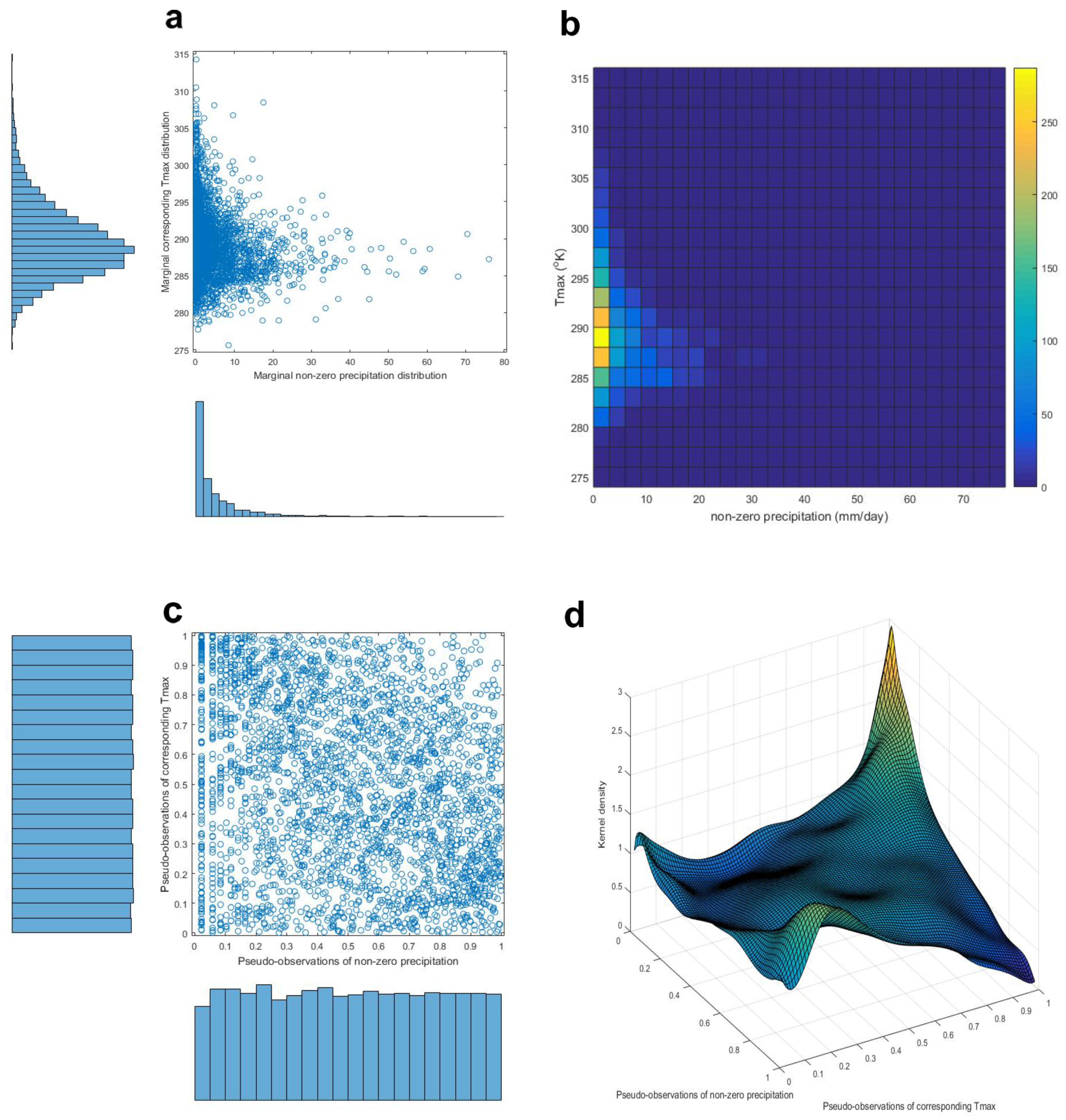
Apart from modeling central tendencies, one of the goals of the present study is to compare future risks of having extreme precipitation and heat wave events to the current risk level. Figure 6 shows the child GEV distributions for precipitation and Tmax at both locations under the RCP4.5 emission scenario.
Table 2 shows three arbitrarily chosen exceedance probability thresholds (0.05, 0.02, and 0.01), the associated values for annual precipitation, and Tmax maxima for both AFB and FBR locations extracted from observations for the 1985–2011 period [33]. The uncertainty is given as the GEV parameter fitting uncertainty and does not include the uncertainty stemming from inaccuracies in the model itself (residual bias, MLR beta non-stationarity, etc.). The values from Table 2 are used as a baseline for comparison with future values.
Table 3 displays the same exceedance probability thresholds and associated values for annual precipitation and Tmax maxima, same as for the past observational datasets, for both locations and both emission scenarios. The probabilities of heat waves are systematically increasing with temporal distance into the future for both emission scenarios. Thus, the 1-in-100-years event for the year 2100, in terms of annual maximum Tmax, shifted from above 318.3K (AFB) in the baseline period to above 320.6 K in the RCP4.5 and above 321.0 K in the RCP8.5 scenario, which is consistent with the change in the mean Tmax values of +2.2 and +2.7 K in the same period for the same emission scenarios (Table 1). Very similar consistency is found for the FBR location between the shift in mean value and the values corresponding to the chosen thresholds in GEV distribution, which reconfirms the robustness of the GEV approach, given that consistent results were obtained using different analytical procedures. On the other hand, the distribution of annual precipitation maxima shifts differently compared to the mean values. For example, the AFB location will have lower magnitude extreme precipitation events (p < 0.01) under the RCP4.5 emission scenario (+0.7%, −10% and −13% for the years 2020, 2050, and 2100, respectively) compared to the baseline, and higher magnitude under the RCP8.5 emission scenario (+15%, +7% and +18% for the years 2020, 2050, and 2100, respectively) compared to the baseline.
On the contrary, a systematic decrease in the precipitation extreme event severities for the FBR location, under both emission scenarios, is found. One-in-one-hundred-years events under the RCP4.5 emission scenario correspond to the values −7%, −8%, and −8%, which are smaller than the values from the baseline period, for the years 2020, 2050, and 2100, respectively, and under RCP8.5 emission scenario −7%, −8% and −8% for the same three future periods. This is also consistent with the direction of change in the mean precipitation daily value in the future for the FBR location, which decreases in both scenarios.
Table 4 shows the increase in future events that corresponded to p < 0.01 (once in 100 days) in the past. Essentially, it shows how much more often these two locations will be witnessing events that were considered to be in the 1% most extreme events in precipitation and Tmax in the past. The results show that both AFB and FBR locations will witness events that, in the past, were considered to be in the 1% most extreme Tmax events ~13–30 times more often. For precipitation, the range found is ~0.05–3 times more often (see Table 4 for details).

3.4. Copulas

One of the goals of this study is to examine the risk of having simultaneous and/or collocated extreme events in terms of precipitation and Tmax. Two locations examined in this study are ~4000 km apart, and the intuitive expectation of having correlated extreme events is low, especially given that precipitation seasonality at these locations is very different. In addition, especially in CA (AFB), precipitation extremes happen in winter months, so the cooccurrence of the two extremes is unlikely. However, as stated earlier, one of the goals of this study was to provide a rigorous, quantitative, and scalable framework for similar analyses in the future, which would likely include more than two locations and perhaps more variables, where analogous arguments based on local meteorology do not necessarily hold. Three tasks were defined: (1) Using empirical copulas, model autocorrelation structures in Tmax and precipitation fields for AFB and FBR locations and for past and future periods. (2) Using empirical copulas, model cross-correlation structures between Tmax and precipitation fields for both locations in past and future time periods. (3) Check the trend in autocorrelation structures to detect eventual sensitivity to climate change.
One problem with the current approaches is that, to model correlation structures using copulas, input data have to be transformed in such a way that the resulting transformed data have a flat distribution. In the case of Tmax, it is easy, e.g., to use CDFs and, instead of using original data, to use their quantiles. However, in the case of precipitation, due to multiple zero values, even if CDFs are used, the resulting distribution of data is not flat, and copula theory cannot be applied directly. Instead, only non-zero precipitation values are used to create copulas, and later the probabilities that precipitation will be non-zero when assessing the probabilities of joint events are separately taken into account.

3.4.1. Tmax Autocorrelation at AFB and FBR

The analysis starts by examining Tmax autocorrelation by analyzing simultaneous distributions of Tmax values in the observational dataset at AFB and FBR. Prior to creating copula structures, Tmax observations are converted into uniformly distributed pseudo-observations using a rank-based approach. Figure 7a shows the marginal and joint distributions of Tmax observations at AFB and FBR, 7b shows a 2D histogram in tile format, 7c shows the marginal and joint distribution of pseudo-observations, and 7d shows the empirical copulas fitted into a joint distribution of pseudo-observations calculated using a 0.03 kernel bandwidth and copula densities evaluated at 100 equi-spaced points in [0,1] range along both axes. A copula is a hyperdimensional structure, and the same approach could be used for more than two locations, if necessary.
A fitted empirical copula is sampled using the Monte-Carlo approach, and 10 million pairs of pseudo-observations of the simultaneous Tmax pairs at both locations, which obey the modeled copula structure generated, and these pseudo-observations are subjected to statistical analysis.
It is found that the probability for Tmax occurring only once in 20 days at both locations is 0.5872% (which means that on ~two days for every year, Tmax recorded at AFB and FBR will be among the 5% warmest days recorded at both sites). It is found that the probability for Tmax occurring only once in 50 days at both locations is 0.0796% (which means that on one day for every ~five years, Tmax recorded at AFB and FBR will be among the 2% warmest days recorded at both sites). It is found that the probability for Tmax occurring only once in 100 days at both locations is 0.0135% (which means that on one day for every ~20 years, Tmax recorded at AFB and FBR will be among the 1% warmest days recorded at both sites). The probability that Tmax occurring only once in 365 days (annual maximum) at both locations is 0.0037% (which means that on one day every ~74 years, Tmax recorded at AFB and FBR will be the actual annual Tmax maximum recorded at both sites). The probability that both sites could experience a 1-in-20-years event simultaneously is essentially zero for these two sites.
One problem in this analysis is that, to estimate frequency of extreme events, it is not only needed to model the tails of the observed distributions at two locations separately but to extrapolate the correlation structure between these tails, which might differ from the correlation structure that describes the observed set of Tmax values. In this analysis, it is assumed that the copula based on actually observed values is stationary and will not change even if never-observed (no-analog-day) events happened. It is concluded that the risk of correlated heat waves at a 1-in-20 intensity at these two sites was negligible in 1985–2015.
The same procedure for all future periods and two emission scenarios was repeated, and it was found that the risk remained similar. Thus, it was concluded that predicted climate change did not affect the risk of correlated extreme Tmax events for those two locations.

3.4.2. Precipitation Autocorrelation at AFB and FBR

Similarly, precipitation auto-correlation structures at AFB and FBR are analyzed, with one difference. As mentioned earlier, the multiple zero precipitation values present a problem for the techniques that convert observations into pseudo-observations. Thus, the modeling copulas were done using a subset of precipitation data, specifically non-zero precipitation values (which also reduced overall number of observations, as the probability that both locations will have non-zero precipitation value was ~1/3). Figure 8a shows the marginal and joint distributions of non-zero precipitation events at AFB and FBR locations in the period 1985–2011, as well as a 2D histogram, the marginal and joint distributions of pseudo-observations, and the modeled copula.
Pseudo-observations (10 M) are, again, simulated using a modeled copula structure and the Monte-Carlo approach. It is found that the probability for precipitation intensity that happens only once in 20 days is 0.0388% (which means that one day every ~7 years precipitation recorded at AFB and FBR will be among 5% highest precipitations recorded at both sites). It is found that the probability for precipitation intensity that happens only once in 50 days is 0.0065% (which means that one day every ~40 years precipitation recorded at AFB and FBR will be among 2% highest precipitations recorded at both sites). It is found that the probability for precipitation intensity that happens only once in 100 days is 1110−4% (which means that one day every ~250 years precipitation recorded at AFB and FBR will be among 1% highest precipitations recorded at both sites).
The probability for precipitation intensity that happens only once in 365 days (annual maximum) is 3.17210−4% (which means that one day every ~850 years precipitations recorded at AFB and FBR will be the annual precipitation maximum recorded at both sites). The probability that 1-in-20-years precipitation events will occur on the same day at these two sites is essentially zero.
Very similar frequencies of occurrences of extreme events in the future were found and demonstrated that climate change does not bring significantly altered probabilities of having extreme simultaneous precipitation events in the future at AFB and FBR.

3.4.3. Tmax/Precipitation Cross-Correlation at AFB

The probabilities that extreme precipitation and Tmax events would occur at AFB and FBR sites were examined separately. Even at a first glance, it looks very unlikely that those two extremes will co-occur, as the rainy season at AFB is happening in the winter, and, in addition to this, rain exhibits a cooling effect, but the analytical steps described above are repeated. Figure 9 shows the marginal and joint distributions of non-zero precipitation events and the corresponding Tmax at AFB location during 1985–2011, as well as a 2D histogram, the marginal and joint distributions of their pseudo-observations, and the modeled copula. It was found that the probability that precipitation and the corresponding Tmax that happen only once in 20 days is 0.0112% (which means that one day every ~25 years precipitation and Tmax recorded at AFB will be among 5% highest precipitations and Tmaxs’ recorded). It was found that the probability that precipitation and corresponding Tmax that happen only once in 50 days is 0.001% (which means that one day every ~266 years precipitation and Tmax recorded at AFB will be among 2% highest precipitations and Tmax recorded). Finally, it was found that the probability that precipitation and the corresponding Tmax that happen only once in 100 days is 1.321510−4% (which means that one day every ~2100 years precipitation and corresponding Tmax recorded at AFB will be among 1% highest precipitations recorded at that site). The probability that precipitation that happens only once in 365 days (annual maximum) is 3.160210−5%, which means that one day every ~8700 years precipitations recorded at AFB will be the maxima for annual precipitation and the corresponding Tmax. Given that the rainy season in CA happens in winter, this finding is not surprising. The probability that 1-in-20-years events will occur on the same day is zero.

3.4.4. Tmax/Precipitation Cross-Correlation at FBR

The same procedure for the FBR site is repeated, and those results are shown in Figure 10. It was found that the probability for precipitation and the corresponding Tmax that happen only once in 20 days is 0.1073% (which means that one day every ~2.5 years precipitation and Tmax recorded at FBR will be among 5% highest precipitations and Tmax recorded). It was found that the probability that precipitation and the corresponding Tmax that happen only once in 50 days is 0.0124% (which means that one day every ~22 years precipitation and Tmax recorded at FBR will be among 2% highest precipitations and Tmax recorded). It was found that the probability for precipitation and the corresponding Tmax that happen only once in 100 days is 0.0018% (which means that one day every ~150 years precipitation and Tmax recorded at FBR will be among 1% highest precipitations recorded at both sites).
The probability that precipitation that happens only once in 365 days (annual maximum) is 4.49 × 10⁻⁴% (which means that one day every ~610 years precipitation recorded at FBR will be the maxima for annual precipitation and Tmax. Interestingly, the probability, despite being low, is much higher than the probability of a co-occurrence of these events at AFB. This is consistent with the fact that precipitation is not as strictly associated with the winter season at FBR, as in the case of AFB. The probability that 1-in-20-years events will occur on the same day is essentially zero.

4. Conclusions

In this study, the effects of climate change on central tendency, tail distributions, correlation structure, and the spatial variability of Tmax and precipitation fields at two locations, AFB and FBR, which represent locations of first-grade military facilities were evaluated. The immediate goal was to inform infrastructural planning, and the second goal was to come up with a robust, reproducible set of methodological steps that could be deployed to analyze effects of climate change on additional or different locations.
A range of analytical techniques, including Bhattacharyya distances, MLR, QDM, GEV, and the Copula theory coupled with Monte-Carlo simulations was applied to create estimates of the future weather at two locations with different climates, as well as to assess probabilities of extreme events and their correlated risks. It was found that Tmax is projected to increase on average by 2.2–2.7 °C at AFB and 1.6–2.2 °C at FBR in the years 2085–2115, based on the combined results from two emission scenarios. Given that the value is lower than the change in average surface temperature on Earth (e.g., [51]), it implies that Tmax and Taverage distributions are projected to change in slightly different ways, which is beyond the scope of this study. It was found that climate change will not induce significant changes in auto- and cross-correlation structures in precipitation and Tmax fields at two studied locations.
It was also analyzed how much more frequently events that correspond to the 1% most extreme events in the baseline period will occur in the future, and it was found that, at both locations, the range of factors for Tmax is ~13–30 and 0.05–3 for precipitation.
Finally, although the analytical framework was developed for the specific purpose of analyzing the risks associated with climate change at two military bases, we believe that it can be extrapolated in a straightforward way to other climate variables and an arbitrary number of other locations, utilizing the hypothetically unlimited hyper-dimensional nature of copulas.

Supplementary Materials

The following are available online at https://www.mdpi.com/2225-1154/8/2/18/s1, Figure S1: Scatter-plot of the Tmax from historical observations for AFB(a) and FBR(b) (Livneh et al. (2013)) along with the best linear fit, Figure S2: Monterey County, CA historical and future temperature trajectories from Cal-Adapt.org, Table S1: List of downscaled CMIP5 GCMs used in the study.

Author Contributions

J.M.T. performed numerical simulations and analysis, and wrote the manuscript. S.C.B. and J.M.T. conceptually designed the study and selected/invented the applied methodology. S.C.B. supervised the work, reviewed and edited the manuscript. All authors have read and agreed to the published version of the manuscript.

Funding

This work was supported by the Strategic Environmental Research and Development Program–SERDP (SERDP Project Number: RC18-1577).

Acknowledgments

We thank Daniel Feldman (LBNL) for help in determining optimal test locations (AFB and FBR), for providing the external hard disk drive used in the study, and helpful discussions. All data used in this study are available upon request. We acknowledge the World Climate Research Programme’s Working Group on Coupled Modelling, which is responsible for CMIP, and we thank the climate modeling groups (listed in Table S1 of this paper) for producing and making available their model output. For CMIP the U.S. Department of Energy’s Program for Climate Model Diagnosis and Intercomparison provides coordinating support and led development of software infrastructure in partnership with the Global Organization for Earth System Science Portals.

Conflicts of Interest

The authors declare no conflict of interest.

References

  1. Parry, M.L.; Rosenzweig, C.; Iglesias, A.; Livermore, M.; Fischer, G. Effects of climate change on global food production under SRES emissions and socio-economic scenarios. Glob. Environ. Chang. A 2004, 14, 53–67. [Google Scholar] [CrossRef]
  2. Patz, J.A.; Campbell-Lendrum, D.; Holloway, T.; Foley, J.A. Impact of regional climate change on human health. Nature 2005, 438, 310–317. [Google Scholar] [CrossRef] [PubMed]
  3. Milly, P.C.D.; Betancourt, J.; Falkenmark, M.; Hirsch, R.M.; Kundzewicz, Z.W.; Lettenmaier, D.P.; Stouffer, R.J. Climate change. Stationarity is dead: Whither water management? Science 2008, 319, 573–574. [Google Scholar] [CrossRef] [PubMed]
  4. Schweikert, A.; Chinowsky, P.; Espinet, X.; Tarbert, M. Climate Change and Infrastructure Impacts: Comparing the Impact on Roads in ten Countries through 2100. Procedia Eng. 2014, 78, 306–316. [Google Scholar] [CrossRef] [Green Version]
  5. Bulkeley, H. Cities and governing of climate change. Annu. Rev. Environ. Res. 2010, 35, 229–253. [Google Scholar] [CrossRef] [Green Version]
  6. Bellard, C.; Bertelsmeier, C.; Leadley, P.; Thuiller, W.; Courchamp, F. Impacts of climate change on the future of biodiversity. Ecol. Lett. 2012, 15, 365–377. [Google Scholar] [CrossRef] [Green Version]
  7. Harris, J.M.; Roach, B.; Environmental, J.M.H. The Economics of Global Climate Change; Global Development and Environment Institute, Tufts University: Massachusetts, MA, USA, 2015. [Google Scholar]
  8. Urry, J. Climate Change and Society; UK Polity Press: Cambridge, UK, 2011. [Google Scholar]
  9. Moss, R.H.; Kravitz, B.; Delgado, A.; Asrar, G.; Brandenbeger, J.; Wigmosta, M.; Preston, K.; Buzan, T.; Gremillion, M.; Shaw, P.; et al. Nonstationarity RC Workshop Report: Nonstationary Weather Patterns and Extreme Events Informing Design and Planning for Long-Lived Infrastructure; Technical Report; Pacific Northwest National Lab: Richland, WA, USA, 2017. [Google Scholar]
  10. Brekke, L.D.; Dettinger, M.D.; Maurer, E.P.; Anderson, M. Significance of model credibility in estimating climate projection distributions for regional hydroclimatological risk assessments. Clim. Chang. 2008, 89, 371–394. [Google Scholar] [CrossRef]
  11. Van Vuuren, D.P.; Edmonds, J.; Kainuma, M.; Riahi, K.; Thomson, A.; Hibbard, K.; Hurtt, G.C.; Kram, T.; Krey, V.; Lamarque, J. The representative concentration pathways: An overview. Clim. Chang. 2011, 109, 5. [Google Scholar] [CrossRef]
  12. Taylor, K.E.; Stouffer, R.J.; Meehl, G.A. An overview of CMIP5 and the experiment design. Bull. Am. Meteorol. Soc. 2012, 93, 485–498. [Google Scholar] [CrossRef] [Green Version]
  13. Andrews, T.; Gregory, J.M.; Webb, M.J.; Taylor, K.E. Forcing, feedbacks and climate sensitivity in CMIP5 coupled atmosphere-ocean climate models. Geophys. Res. Lett. 2012, 39, L09712. [Google Scholar] [CrossRef] [Green Version]
  14. Ntegeka, V.; Baguis, P.; Roulin, E.; Willems, P. Developing tailored climate change scenarios for hydrological impact assessments. J. Hydrol. 2014, 508, 307–321. [Google Scholar] [CrossRef]
  15. Barros, A.P.; Lettenmaier, D.P. Dynamic modeling of orographically induced precipitation. Rev. Geophys. 1994, 32, 265–284. [Google Scholar] [CrossRef]
  16. Leung, L.R.; Ghan, S.J. A subgrid parameterization of orographic precipitation. Theor. Appl. Climatol. 1995, 52, 95–118. [Google Scholar] [CrossRef]
  17. Gleckler, P.J.; Taylor, K.E.; Doutriaux, C. Performance metrics for climate models. J. Geophys. Res. 2008, 113, D06104. [Google Scholar] [CrossRef]
  18. Rupp, D.E.; Abatzoglou, J.T.; Hegewisch, K.C.; Mote, P.W. Evaluation of CMIP5 20th century climate simulations for the Pacific Northwest USA. J. Geophys. Res. Atmos. 2013, 118, 10884–10906. [Google Scholar] [CrossRef]
  19. Pierce, D.W.; Cayan, D.R.; Thrasher, B.L. Statistical downscaling using localized constructed analogs (LOCA). J. Hydrometerol. 2014, 15, 2558–2586. [Google Scholar] [CrossRef]
  20. Christensen, J.H.; Boberg, F.; Christensen, O.B.; Lucas-Picher, P. On the need for bias correction of regional climate change projections of temperature and precipitation. Geophys. Res. Lett. 2008, 35, L20709. [Google Scholar] [CrossRef]
  21. Mearns, L.O.; Arritt, R.; Biner, S.; Bukovsky, M.S.; McGinnis, S.; Caya, S.S.D.; Correia, J., Jr.; Flory, D.; Gutowski, W.; Takle, E.S.; et al. The North American Regional Climate Change Assessment Program: Overview of phase I results. Bull. Am. Meteor. Soc. 2012, 93, 1337–1362. [Google Scholar] [CrossRef]
  22. Sillmann, J.; Kharin, V.V.; Zhang, X.; Zwiers, F.W.; Bronaugh, D. Climate extremes indices in the CMIP5 multimodel ensemble: Part 1. Model evaluation in the present climate. J. Geophys. Res. Atmos. 2013, 118, 1716–1733. [Google Scholar] [CrossRef]
  23. Cannon, A.J.; Sobie, S.R.; Murdock, T.Q. Bias Correction of GCM Precipitation by Quantile Mapping: How Well Do Methods Preserve Changes in Quantiles and Extremes? J. Clim. 2015, 28, 6938–6959. [Google Scholar] [CrossRef]
  24. Ehret, U.; Zehe, E.; Wulfmeyer, V.; Warrach-Sagi, K.; Liebert, J. HESS opinions: “Should we apply bias correction to global and regional climate model data?”. Hydrol. Earth Syst. Sci. 2012, 16, 3391–3404. [Google Scholar] [CrossRef] [Green Version]
  25. Maraun, D. Nonstationarities of regional climate model biases in European seasonal mean temperature and pre- cipitation sums. Geophys. Res. Lett. 2012, 39, L06706. [Google Scholar] [CrossRef] [Green Version]
  26. Maraun, D. Bias correction, quantile mapping, and downscaling: Revisiting the inflation issue. J. Clim. 2013, 26, 2137–2143. [Google Scholar] [CrossRef] [Green Version]
  27. Gudmundsson, L.; Bremnes, J.B.; Haugen, J.E.; Engen-Skaugen, T. Technical note: Downscaling RCM precipitation to the station scale using statistical transformations—A comparison of methods. Hydrol. Earth Syst. Sci. 2012, 16, 3383–3390. [Google Scholar] [CrossRef] [Green Version]
  28. Teutschbein, C.; Seibert, J. Bias correction of regional climate model simulations for hydrological climate-change impact studies: Review and evaluation of different methods. J. Hydrol. 2012, 456–457, 12–29. [Google Scholar] [CrossRef]
  29. Teutschbein, C.; Seibert, J. Is bias correction of regional climate model (RCM) simulations possible for non-stationary conditions? Hydrol. Earth Syst. Sci. 2013, 17, 5061–5077. [Google Scholar] [CrossRef] [Green Version]
  30. Hagemann, S.; Chen, C.; Haerter, J. Impact of a statistical bias correction on the projected hydrological changes obtained from three GCMs and two hydrology models. J. Hydrometeorol. 2011, 12, 556–578. [Google Scholar] [CrossRef]
  31. Themeßl, M.J.; Gobiet, A.; Heinrich, G. Empirical- statistical downscaling and error correction of re- gional climate models and its impact on the climate change signal. Clim. Chang. 2012, 112, 449–468. [Google Scholar] [CrossRef]
  32. Maurer, E.P.; Pierce, D.W. Bias correction can modify climate model simulated precipitation changes without adverse effect on the ensemble mean. Hydrol. Earth Syst. Sci. 2014, 18, 915–925. [Google Scholar] [CrossRef] [Green Version]
  33. Livneh, B.; Rosenberg, E.A.; Lin, C.; Nijssen, B.; Mishra, V.; Andreadis, K.M.; Maurer, E.P.; Lettenmaier, D.P. A long-term hydrologically based dataset of land surface fluxes and states for the conterminous United States: Update and extensions. J. Clim. 2013, 26, 9384–9392. [Google Scholar] [CrossRef]
  34. Haas, T.C. Lognormal and moving window methods of estimating acid deposition. J. Am. Stat. Assoc. 1990, 85, 950–963. [Google Scholar] [CrossRef]
  35. Tadić, J.M.; Qiu, X.; Miller, S.; Michalak, A.M. Spatio-temporal approach to moving window block kriging of satellite data v1.0. Geosci. Model Dev. 2017, 10, 709–720. [Google Scholar] [CrossRef] [Green Version]
  36. California Water Commission Techical Reference. 2016. Available online: https://water.ca.gov/LegacyFiles/economics/downloads/EAS_Docs/WSIP_Draft_TechRefDoc_Compiled.pdf (accessed on 21 January 2020).
  37. Mauritsen, T.; Stevens, B.; Roeckner, E.; Crueger, T.; Esch, M.; Giorgetta, M.; Haak, H.; Jungclaus, J.; Klocke, D.; Matei, D.; et al. Tuning the climate of a global model. J. Adv. Modeling Earth Syst. 2012, 4. [Google Scholar] [CrossRef]
  38. Kharin, V.V.; Zwiers, F.W.; Zhang, X.; Wehner, M. Changes in temperature and precipitation extremes in the CMIP5 ensemble. Clim. Chang. 2013, 119, 345–357. [Google Scholar] [CrossRef]
  39. Van den Dool, H.M. Searching for analogues, how long must we wait? Tellus 1994, 46A, 314–324. [Google Scholar] [CrossRef]
  40. Wood, A.W.; Leung, L.R.; Sridhar, V.; Lettenmaier, D.P. Hydrologic implications of dynamical and statistical approaches to downscaling climate model outputs. Clim. Chang. 2004, 62, 189–216. [Google Scholar] [CrossRef]
  41. Maurer, E.P. The utility of daily large-scale climate data in the assessment of climate change impacts on daily streamflow in California. Hydrol. Earth Syst. Sci. 2010, 14, 1125–1138. [Google Scholar] [CrossRef] [Green Version]
  42. Abatzoglou, J.T.; Brown, T.J. A comparison of statis- tical downscaling methods suited for wildfire applications. Int. J. Climatol. 2012, 32, 772–780. [Google Scholar] [CrossRef]
  43. Bhattacharyya, A. On a measure of divergence between two statistical populations defined by their probability distributions. Bull. Calcutta Math. Soc. 1943, 35, 99–109. [Google Scholar]
  44. Coles, S. An Introduction to Statistical Modeling of Extreme Values; Springer: London, UK, 2001; ISBN 1-85233-459-2. [Google Scholar]
  45. Rudin, W. Principles of Mathematical Analysis; McGraw Hill: New York, NY, USA, 1976; pp. 89–90. [Google Scholar]
  46. Charpentier, A.; Fermanian, J.-D.; Scaillet, O. The Estimation of Copulas: Theory and Practice. In Copulas: From Theory to Applications in Finance; Rank, J., Ed.; Risk Books: London, UK, 2007; pp. 35–62. [Google Scholar]
  47. Schmidt, T. Coping with Copulas, in: Copulas—From Theory to Application in Finance; Risk Books: London, UK, 2007; pp. 3–34. [Google Scholar]
  48. Sklar, A. Fonctions de Repartition a n Dimensions et Leurs Marges; Public instruction Statistics University: Paris, France, 1959; Volume 8, pp. 229–231. [Google Scholar]
  49. Chen, S.X. A beta kernel estimation for density functions. Comput. Stat. Data Anal. 1999, 31, 131–135. [Google Scholar] [CrossRef]
  50. Brown, B.M.; Chen, S.X. Beta-Bernstein smoothing for regression curves with compact supports. Scand. J. Stat. 1999, 26, 47–59. [Google Scholar] [CrossRef]
  51. Brown, P.T.; Caldeira, K. Greater future global warming inferred from Earth’s recent energy budget. Nature 2017, 552, 45. [Google Scholar] [CrossRef] [PubMed]
Figure 1. The flow diagram of the analysis. (1) Input data (observational and model data) are first converted into empirical PDFs and CDFs. (2) PDFs and CDFs are subjected to MLR to reconstruct observational CDFs using model CDFs. Next, (3) QDM is applied to observational data using past and future CDFs. (4) Once bias-corrected future data are available, we apply GEV theory and examine change in likelihood of extreme events. Finally, (5) copula theory is applied to assess whether climate change increases risk of simultaneous or collocated extreme events.
Climate 08 00018 g001
Figure 2. Bhattacharyya coefficients for precipitation (ad) and Tmax (eh) modeled PDFs compared to the baseline period (1985–2015). (b,f) correspond to period centered around year 2020, (c,g) centered around 2050, and (d,h) centered around 2100. Two column plots (bd for precipitation and fh for Tmax) correspond to two emission scenarios, RCP4.5 (first column) and RCP8.5 (second column).
Climate 08 00018 g002
Figure 3. Selected Bhattacharyya coefficient plots for precipitation (a,b) and Tmax (c,d) PDFs inter compared between model ensemble members. (a) Precipitation PDF inter-comparison for 2035–2065, RCP4.5. (b) Precipitation PDF inter-comparison for 2035–2065, RCP8.5. (c) Tmax PDF inter-comparison for 2035–2065, RCP4.5. (d) Tmax PDF inter-comparison for 2035–2065, RCP8.5.
Climate 08 00018 g003
Figure 4. MLR beta coefficients (and intercepts) (a,b) obtained by reconstructing observational precipitation and Tmax CDF using 32 model outputs downscaled by LOCA, for the 1985–2011 period. Figure 4c,d shows observational and reconstructed CDFs for precipitation (c) and Tmax (d).
Climate 08 00018 g004
Figure 5. Exemplary CDFs for precipitation (a,b) and PDFs for Tmax (c,d) for the AFB location, comparing the 2035–2065 period to the baseline period.
Climate 08 00018 g005
Figure 6. (a) GEV PDF for annual precipitation maximum values for 2035–2065, AFB, under RCP4.5 emission scenario, (b) GEV PDF for annual Tmax maximum values for 2035–2065, AFB, under RCP4.5 emission scenario, (c) GEV PDF for annual precipitation maximum values for 2035–2065, FBR, under RCP4.5 emission scenario, and (d) GEV PDF for annual Tmax maximum values for 2035–2065, FBR, under RCP4.5 emission scenario.
Climate 08 00018 g006
Figure 7. (a) Marginal and joint distribution of observations of Tmax at AFB and FBR during 1985–2011 period. (b) 2D histogram shown in tile format. (c) Marginal and joint distributions of Tmax pseudo observations, prepared as input to copula-modeling. (d) Fitted empirical copula.
Climate 08 00018 g007
Figure 8. (a) Marginal and joint distribution of precipitation observations at AFB and FBR during 1985–2011 period. (b) 2D histogram shown in tile format. (c) Marginal and joint distributions of precipitation pseudo-observations, prepared as input to copula-modeling. (d) Fitted empirical copula.
Climate 08 00018 g008
Figure 9. (a) Marginal and joint distribution of observations of non-zero precipitation and corresponding Tmax at AFB, during 1985–2011 period. (b) 2D histogram shown in tile format. (c) Marginal and joint distributions of non-zero precipitation and Tmax pseudo-observations, prepared as input to copula modeling. (d) Fitted empirical copula.
Climate 08 00018 g009
Figure 10. (a) Marginal and joint distribution of observations of non-zero precipitation and corresponding Tmax at FBR, during 1985–2011 period. (b) 2D histogram shown in tile format. (c) Marginal and joint distributions of non-zero precipitation and Tmax pseudo-observations, prepared as input to copula-modeling. (d) Fitted empirical copula.
Climate 08 00018 g010
Table 1. Changes in the average daily precipitation and the maximum daily temperature (Tmax) values (future-past) for three future periods centered around the years 2020, 2050, and 2100, derived from bias-corrected future projections using Multi-Linear Regression (MLR) and past observations, for two emission scenarios (RCP4.5 and RCP8.5).
AFBFBR
RCP4.5RCP8.5RCP4.5RCP8.5
Year (Centered Around)Precipitation (mm/day) (Delta)Tmax (°C) (Delta)Precipitation (mm/Day) (Delta)Tmax (°C) (Delta)Precipitation (mm/Day) (Delta)Tmax (°C) (Delta)Precipitation (mm/Day) (Delta)Tmax (°C) (Delta)
2020+0.1+1.1+0.2+1.1−0.5+0.9−0.3+0.1
2050−0.0+2.0+0.0+1.9−0.4+1.2−0.3+1.5
2100−0.1+2.2+0.0+2.7−0.5+1.6−0.4+2.2
Table 2. Exceedance probability thresholds and associated values taken from observations (1985–2011) of the Travis Airforce Base (AFB) and Fort Bragg (FBR) locations, based on the Generalized Extreme Value (GEV) distribution for precipitation and Tmax. The uncertainty is reported as 95% Confidence Intervals (CI).
Observations, 1985–2011
AFBFBR
Exceedance Probability (1985–2015)Precipitation (mm/Day) (95% CI)Tmax (K) (95% CI)Precipitation (mm/Day) (95% CI)Tmax (K) (95% CI)
P (0.05)70.4 (43.9–131.3)317.2 (315.1–320.3)94.9 (66.3–152.4)313.7 (311.5–317.6)
P (0.02)80.8 (46.0–183.1)317.9 (315.4–322.1)109.0 (70.1–204.7)314.1 (311.6–319.3
P (0.01)88.4 (47.1–233.4)318.3 (315.6–323.5)119.8 (72.5–254.9)314.3 (311.6–320.4)
Table 3. Exceedance probability thresholds and associated values taken from bias-corrected modeled precipitation and Tmax values for three future periods (centered around the years 2020, 2050, and 2100), for both AFB and FBR locations under two emission scenarios, based on GEV distribution. The uncertainty is reported as 95% Confidence Intervals (CI).
RCP4.5RCP8.5
Year (Centered Around)Exceedance ProbabilityPrecipitation (mm/Day) (95% CI)Tmax (K) (95% CI)Precipitation (mm/Day) (95% CI)Tmax (K) (95% CI)
AFB2005–2035P (0.05)73.8 (45.7–137.8)318.2 (316.1–321.8)80.2 (47.7–159.5)318.2 (316.2–321.6)
P (0.02)83.0 (47.5–185.5)318.9 (316.3–324.1)92.7 (50.0–227.8)319.0 (316.4–323.6)
P (0.01)89.1 (48.4–229.2)319.4 (316.4–325.9)101.7 (51.2–295.5)319.5 (316.6–325.2)
2035–2065P (0.05)67.3 (44.3–109.1)319.1 (317.0–322.6)76.5 (46.2–138.0)319.1 (317.0–322.5)
P (0.02)74.7 (46.5–135.1)319.8 (317.3–324.9)87.6 (49.9–183.3)319.9 (317.3–324.5)
P (0.01)79.5 (47.6–155.9)320.3 (317.4–326.6)95.2 (50.4–223.6)320.3 (317.4–325.9)
2085–2115P (0.05)66.0 (43.4–103.2)319.3 (317.2–322.7)80.45 (46.4–155.8)319.9 (317.8–323.2)
P (0.02)72.8 (45.7–123.5)320.1 (317.5–324.9)94.3 (49.5–219.4)320.6 (318.1–325.0)
P (0.01)77.0 (46.9–138.5)320.6 (317.7–326.6)104.3 (51.1–280.1)321.0 (318.2–326.4)
Year (centered around)Exceedance ProbabilityPrecipitation (mm/day) (95% CI)Tmax (K) (95% CI)Precipitation (mm/day) (95% CI)Tmax (K) (95% CI)
FBR2005–2035P (0.05)95.8 (65.9–140.6)314.5 (312.4–318.5)91.3 (64.1–136.3)313.9 (311.7–317.8)
P (0.02)105.6 (69.9–164.4)314.9 (312.4–320.0)103.2 (68.4–168.8)314.3 (311.8–319.5)
P (0.01)111.6 (72.1–181.4)315.0 (312.5–321.1)111.4 (71.0–195.6)314.5 (311.8–320.6)
2035–2065P (0.05)93.5 (63.4–134.7)314.9 (312.7–318.7)92.5 (65.1–134.8)315.3 (313.1–319.1)
P (0.02)103.4 (69.6–157.5)315.3 (312.8–320.2)103.1 (69.4–161.4)315.8 (313.3–320.8)
P (0.01)109.6 (72.0–173.8)315.5 (312.9–321.3)110.1 (71.8–181.8)316.1 (313.3–322.0)
2085–2115P (0.05)94.6 (66.4–135.5)315.3 (313.1–319.4)93.0 (65.3–134.2)315.9 (313.7–319.8)
P (0.02)104.1 (70.5–157.1)315.7 (313.2–321.1)103.2 (69.6–158.0)316.4 (313.9–321.4)
P (0.01)109.9 (72.8–172.2)315.9 (313.2–322.2)109.6 (72.0–175.4)316.6 (313.9–322.5)
Table 4. The ratio of probability of the extreme event in the future that corresponded to p < 0.01 in the past and its probability for three future periods (centered around the years 2020, 2050, and 2100), for both AFB and FBR locations under two emission scenarios, based on GEV distribution. The uncertainty is reported as 95% Confidence Intervals (CI).
AFBFBR
Precipitation (mm/Day) (95% CI)Tmax (K) (95% CI)Precipitation (mm/Day) (95% CI)Tmax (K) (95% CI)
RCP4.5RCP8.5RCP4.5RCP8.5RCP4.5RCP8.5RCP4.5RCP8.5
2005–20351.09 (0–16.5)2.77 (0–20)4.35 (0–21.4)4.63 (0–21.5)0.30 (0–10)0.47 (0–8)7.58 (0–35.5)1.86 (0–26)
2035–20650.20 (0–11)1.87 (0–17)11.35 (0–31.1)11.63 (0–31.5)0.23 (0–9)0.33 (0–8)11.83 (0–38)17.65 (0–41.5)
2085–21150.06 (0–10)2.97 (0–19)13.60 (0–33.4)22.45 (0.7–42.5)0.21 (0–9)0.25 (0–9)19.98 (0–45)31.04 (0–52.5)

