Algorithm to Predict the Rainfall Starting Point as a Function of Atmospheric Pressure, Humidity, and Dewpoint


Abstract
1. Introduction
2. Materials and Methods
2.1. The Clausius–Clapeyron Relation
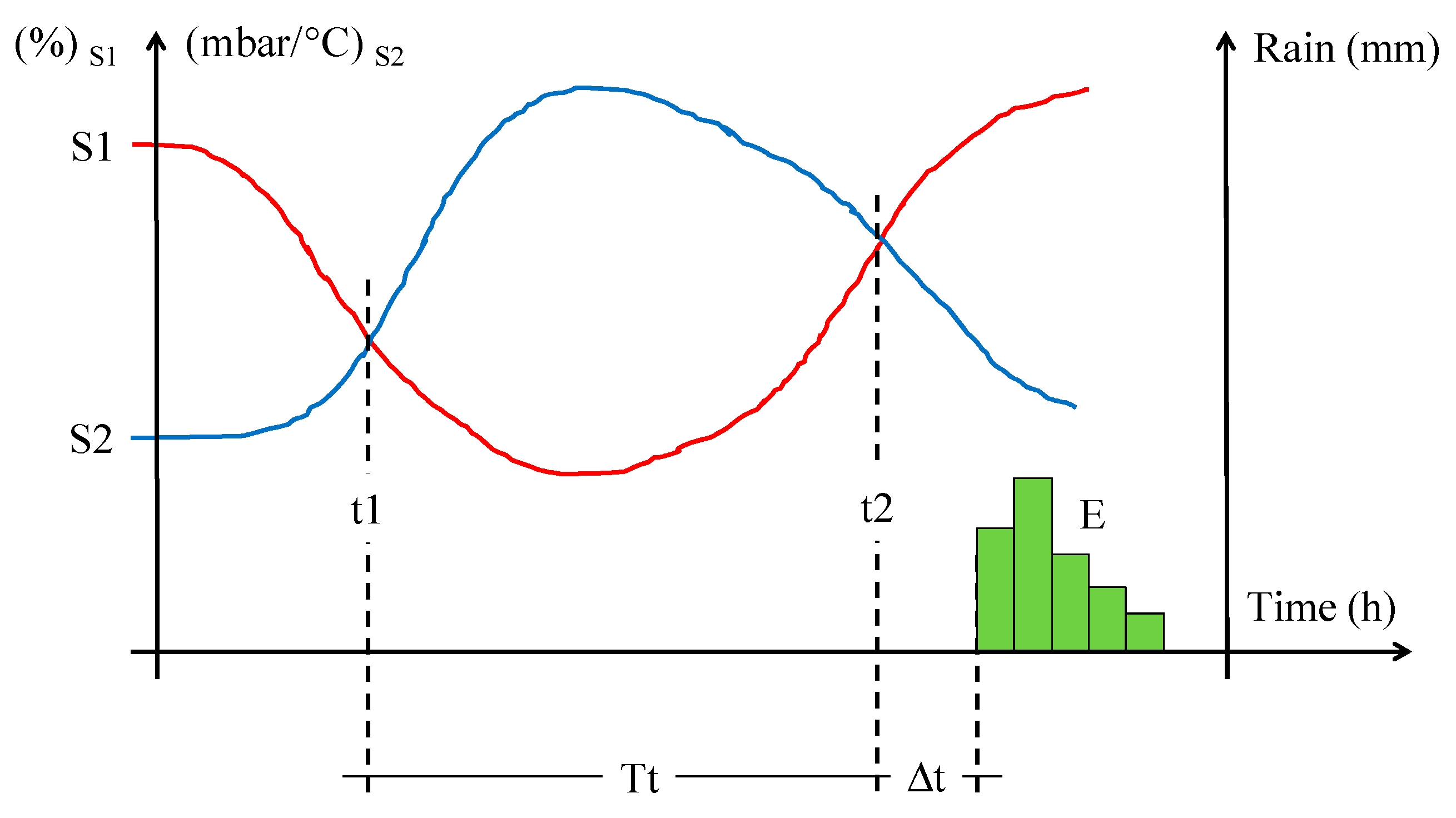
2.2. The Proposed Model
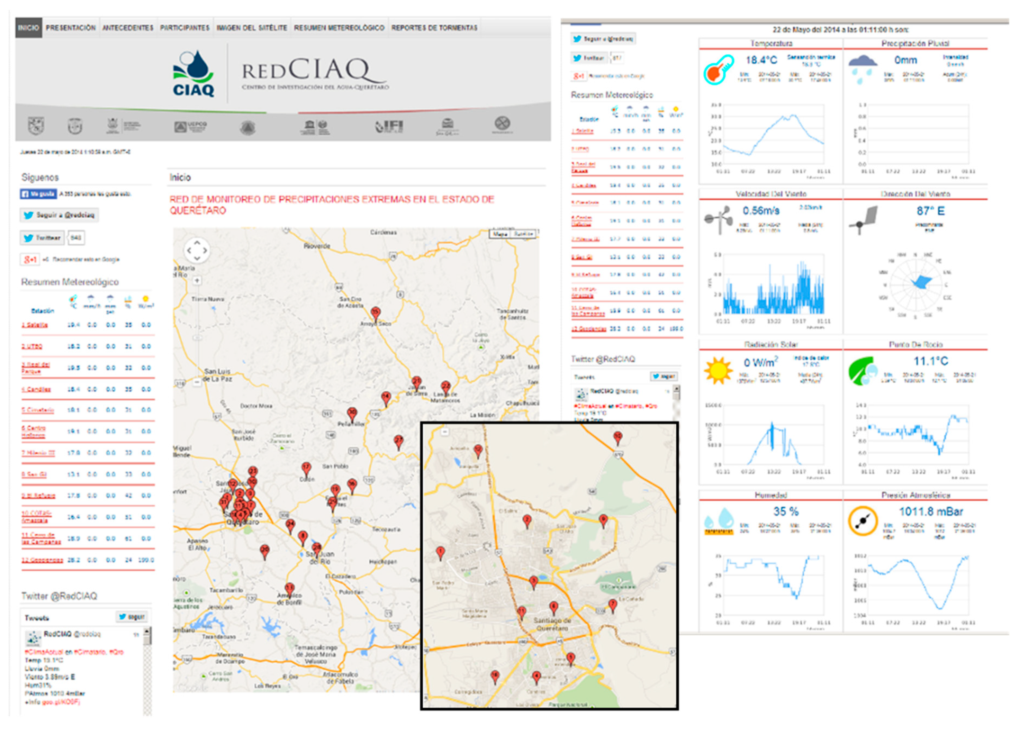
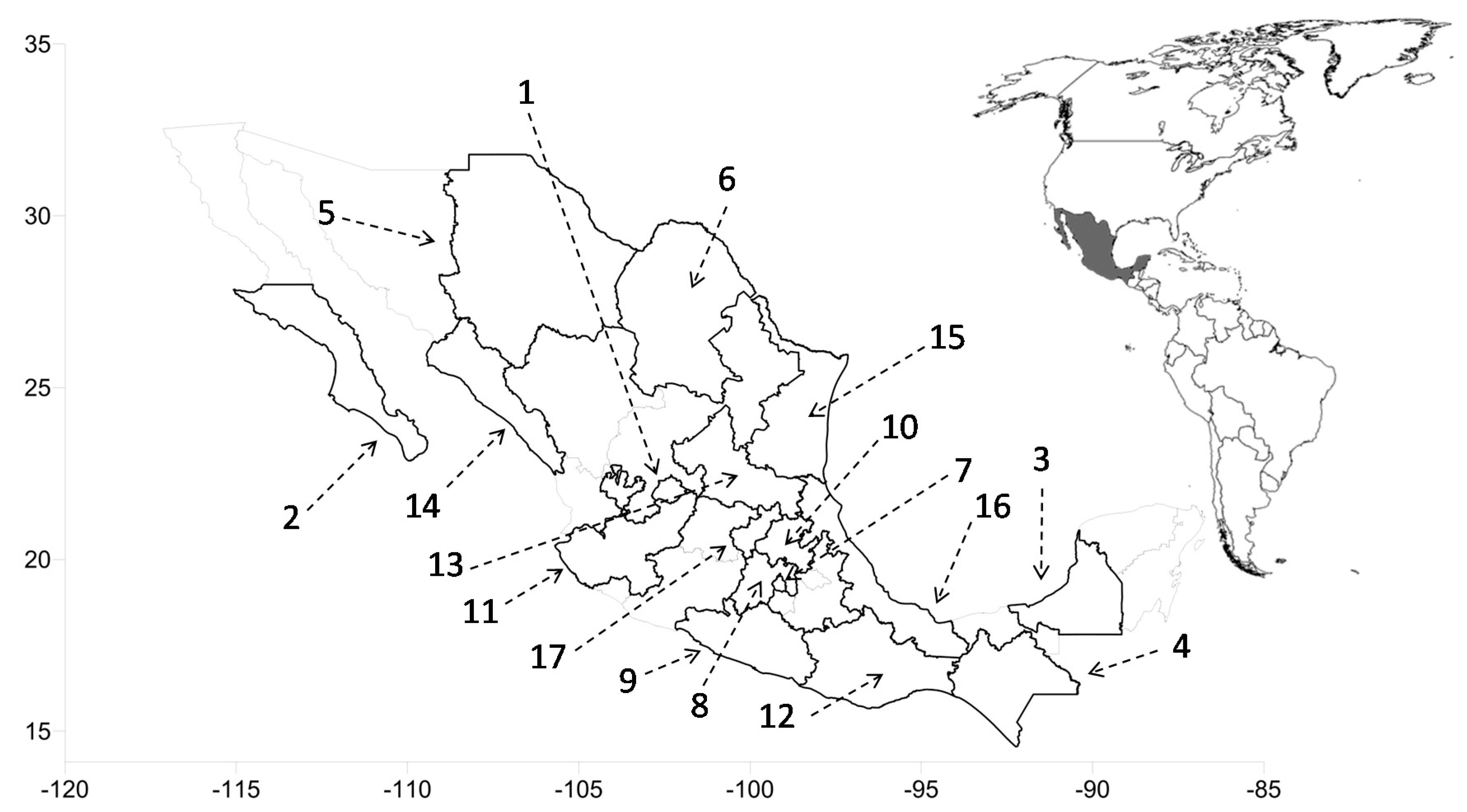
2.3. The Precipitation Network RedCIAQ
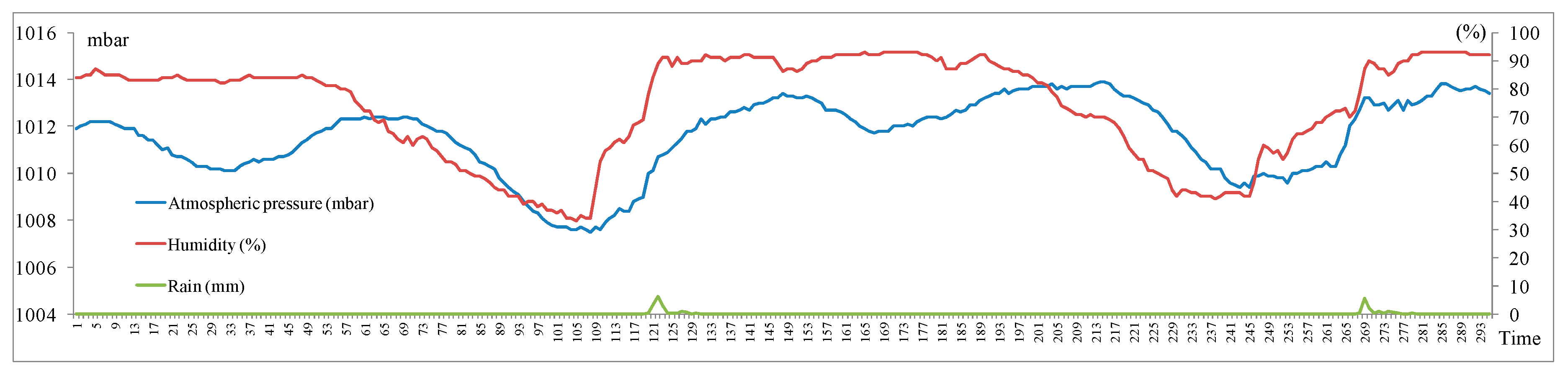
3. Results
4. Discussion
5. Conclusions
Author Contributions
Funding
Acknowledgments
Conflicts of Interest
Appendix A

| Id | Name | Long | Lat | Id | Name | Long | Lat |
|---|---|---|---|---|---|---|---|
| 1 | Chulavista | −100.47 | 20.63 | 18 | Ezequiel Montes | −99.90 | 20.67 |
| 2 | Belén | −100.41 | 20.65 | 19 | Huimilpan | −100.27 | 20.37 |
| 3 | Real del Parque | −100.40 | 20.61 | 20 | Landa de Matamoros | −99.32 | 21.18 |
| 4 | Candiles | −100.40 | 20.55 | 21 | Pedro Escobedo | −100.14 | 20.50 |
| 5 | Cimatario | −100.38 | 20.56 | 22 | San Joaquín | −100.01 | 20.38 |
| 6 | Centro histórico | −100.39 | 20.59 | 23 | San Juan del Rio | −99.97 | 20.39 |
| 7 | Milenio III | −100.35 | 20.59 | 24 | Tequisquiapan | −99.91 | 20.61 |
| 8 | San gil | −100.44 | 20.70 | 25 | Toliman | −99.93 | 20.90 |
| 9 | El refugio | −100.35 | 20.65 | 26 | Viñedos | −100.49 | 20.61 |
| 10 | COTAS Amazcala | −100.34 | 20.71 | 27 | El esparrago | −100.01 | 20.38 |
| 11 | Cerro de las Campanas | −100.41 | 20.59 | 28 | Santa Rosa Jáuregui | −100.45 | 20.74 |
| 12 | Amealco de Bonfil | −100.14 | 20.19 | 29 | Unión de Ejidos | −100.23 | 20.65 |
| 13 | Pinal de Amoles | −99.63 | 21.14 | 30 | Joaquín Herrera | −99.57 | 20.92 |
| 14 | Arroyo seco | −99.69 | 21.55 | 31 | Juriquilla | −100.45 | 20.72 |
| 15 | Cadereyta de Montes | −99.81 | 20.70 | 32 | UAQ Aeropuerto | −100.37 | 20.62 |
| 16 | Colon | −100.05 | 20.78 | 33 | Pasteur y 57 | −100.38 | 20.58 |
| 17 | Corregidora | −100.43 | 20.55 | 34 | CICATA QRO IPN | −100.37 | 20.57 |
References
- CENAPRED. Disasters in Mexico: Social and Economic Impacts (1980–2014); Centro Nacional de Prevencion de Desastres: Secretaría de Gobernacion, Mexico, 2016. [Google Scholar]
- Gutierrez-Lopez, A.; Fortanell Trejo, M.; Albuquerque Gonzalez, N.; Bravo Prado, F. Análisis de la variabilidad espacial en la precipitación en la zona metropolitana de Querétaro empleando ecuaciones de anisotropía. In Investigaciones Geográficas; Instituto de Geografia, Universidad Autonoma de Mexico: Ciudad de México, Mexico, 2019. [Google Scholar] [CrossRef]
- Lepore, C.; Allen, J.; Tippett, M. Relationships between Hourly Rainfall Intensity and Atmospheric Variables over the Contiguous United States. J. Clim. 2016, 29, 3181–3197. [Google Scholar] [CrossRef]
- Saltzman, B. On the Maintenance of the Large-Scale Quasi-Permanent Disturbances in the Atmosphere. Tellus 1959, 11, 425–431. [Google Scholar] [CrossRef]
- Saltzman, B. Dynamical Paleoclimatology, 1st ed.; Academic Press: New York, NY, USA, 2002. [Google Scholar]
- Lorenz, E. Deterministic Nonperiodic Flow. J. Atmos. Sci. 1963, 20, 130–141. [Google Scholar] [CrossRef]
- Berg, P.; Haerter, J. Unexpected increase in precipitation intensity with temperature—A result of mixing of precipitation types? Atmos. Res. 2013, 119, 56–61. [Google Scholar] [CrossRef]
- Holley, D.; Dorling, S.; Steele, C.; Earl, N. A climatology of convective available potential energy in Great Britain. Int. J. Climatol. 2014, 34, 3811–3824. [Google Scholar] [CrossRef]
- Lekouch, I.; Lekouch, K.; Muselli, M.; Mongruel, A.; Kabbachi, B.; Beysens, D. Rooftop dew, fog and rain collection in southwest Morocco and predictive dew modeling using neural networks. J. Hydrol. (Amst.) 2012, 448, 60–72. [Google Scholar] [CrossRef]
- Park, I.; Min, S. Role of Convective Precipitation in the Relationship between Subdaily Extreme Precipitation and Temperature. J. Clim. 2017, 30, 9527–9537. [Google Scholar] [CrossRef]
- Dyson, L.; van Heerden, J.; Sumner, P. A baseline climatology of sounding-derived parameters associated with heavy rainfall over Gauteng, South Africa. Int. J. Climatol. 2014, 35, 114–127. [Google Scholar] [CrossRef]
- Omotosho, J. Equivalent potential temperature and dust haze forecasting at Kano, Nigeria. Atmos. Res. 1989, 23, 163–178. [Google Scholar] [CrossRef]
- Puvaneswaran, M. Climatic classification for queensland using multivariate statistical techniques. Int. J. Climatol. 1990, 10, 591–608. [Google Scholar] [CrossRef]
- Damrath, U.; Doms, G.; Frühwald, D.; Heise, E.; Richter, B.; Steppeler, J. Operational quantitative precipitation forecasting at the German Weather Service. J. Hydrol. (Amst.) 2000, 239, 260–285. [Google Scholar] [CrossRef]
- Rasouli, K.; Hsieh, W.; Cannon, A. Daily streamflow forecasting by machine learning methods with weather and climate inputs. J. Hydrol. (Amst.) 2012, 414, 284–293. [Google Scholar] [CrossRef]
- Moon, S.; Kim, Y.; Lee, Y.; Moon, B. Application of machine learning to an early warning system for very short-term heavy rainfall. J. Hydrol. (Amst.) 2019, 568, 1042–1054. [Google Scholar] [CrossRef]
- Zahraei, A.; Hsu, K.; Sorooshian, S.; Gourley, J.; Hong, Y.; Behrangi, A. Short-term quantitative precipitation forecasting using an object-based approach. J. Hydrol. (Amst.) 2013, 483, 1–15. [Google Scholar] [CrossRef]
- Li, P.; Lai, E. Short-range quantitative precipitation forecasting in Hong Kong. J. Hydrol. (Amst.) 2004, 288, 189–209. [Google Scholar] [CrossRef]
- Carrera-Hernández, J.; Gaskin, S. Spatio temporal analysis of daily precipitation and temperature in the Basin of Mexico. J. Hydrol. (Amst.) 2007, 336, 231–249. [Google Scholar] [CrossRef]
- Carter, M.; Elsner, J.; Bennett, S. A quantitative precipitation forecast experiment for Puerto Rico. J. Hydrol. (Amst.) 2000, 239, 162–178. [Google Scholar] [CrossRef]
- Valverde Ramírez, M.; de Campos Velho, H.; Ferreira, N. Artificial neural network technique for rainfall forecasting applied to the São Paulo region. J. Hydrol. (Amst.) 2005, 301, 146–162. [Google Scholar] [CrossRef]
- Hou, T.; Kong, F.; Chen, X.; Lei, H. Impact of 3DVAR Data Assimilation on the Prediction of Heavy Rainfall over Southern China. Adv. Meteorol. 2013, 2013, 129642. [Google Scholar] [CrossRef]
- Wang, J.; Gaffen, D. Late-Twentieth-Century Climatology and Trends of Surface Humidity and Temperature in China. J. Clim. 2001, 14, 2833–2845. [Google Scholar] [CrossRef]
- Suparta, W.; Alhasa, K.; Singh, M. Estimation water vapor content using the mixing ratio method and validated with the ANFIS PWV model. J. Phys. Conf. Ser. 2017, 852, 012041. [Google Scholar] [CrossRef]
- Camuffo, D. Theoretical Grounds for Humidity. In Microclimate for Cultural Heritage; Elsevier: Amsterdam, The Netherlands, 2014; Chapter 2A; pp. 49–76. ISBN 9780444632982. [Google Scholar] [CrossRef]
- Pumo, D.; Carlino, G.; Blenkinsop, S.; Arnone, E.; Fowler, H.; Noto, L. Sensitivity of extreme rainfall to temperature in semi-arid Mediterranean regions. Atmos. Res. 2019, 225, 30–44. [Google Scholar] [CrossRef]
- Capparelli, A. Fisicoquímica Básica, 1st ed.; Universidad Nacional La Plata Argentina: La Plata, Argentina, 2013. [Google Scholar]
- Van der Dussen, J.; de Roode, S.; Siebesma, A. Factors Controlling Rapid Stratocumulus Cloud Thinning. J. Atmos. Sci. 2014, 71, 655–664. [Google Scholar] [CrossRef]
- Romps, D. Clausius–Clapeyron Scaling of CAPE from Analytical Solutions to RCE. J. Atmos. Sci. 2016, 73, 3719–3737. [Google Scholar] [CrossRef]
- Agard, V.; Emanuel, K. Clausius–Clapeyron Scaling of Peak CAPE in Continental Convective Storm Environments. J. Atmos. Sci. 2017, 74, 3043–3054. [Google Scholar] [CrossRef]
- Lorenz, D.; DeWeaver, E. The Response of the Extratropical Hydrological Cycle to Global Warming. J. Clim. 2007, 20, 3470–3484. [Google Scholar] [CrossRef]
- Romps, D. An Analytical Model for Tropical Relative Humidity. J. Clim. 2014, 27, 7432–7449. [Google Scholar] [CrossRef]
- Chang, W.; Stein, M.; Wang, J.; Kotamarthi, V.; Moyer, E. Changes in Spatiotemporal Precipitation Patterns in Changing Climate Conditions. J. Clim. 2016, 29, 8355–8376. [Google Scholar] [CrossRef]
- Lenderink, G.; Barbero, R.; Loriaux, J.; Fowler, H. Super-Clausius–Clapeyron Scaling of Extreme Hourly Convective Precipitation and Its Relation to Large-Scale Atmospheric Conditions. J. Clim. 2017, 30, 6037–6052. [Google Scholar] [CrossRef]
- Bürger, G.; Heistermann, M.; Bronstert, A. Towards Subdaily Rainfall Disaggregation via Clausius–Clapeyron. J. Hydrometeorol. 2014, 15, 1303–1311. [Google Scholar] [CrossRef]
- Peleg, N.; Marra, F.; Fatichi, S.; Molnar, P.; Morin, E.; Sharma, A.; Burlando, P. Intensification of Convective Rain Cells at Warmer Temperatures Observed from High-Resolution Weather Radar Data. J. Hydrometeorol. 2018, 19, 715–726. [Google Scholar] [CrossRef]
- Velasco, S.; Fernández-Pineda, C. Sobre la obtención de la ecuación de Clapeyron-Clausius. Rev. Española Física 2008, 22, 7–14. [Google Scholar]
- Seidel, T.; Grant, A.; Pszenny, A.; Allman, D. Dewpoint and Humidity Measurements and Trends at the Summit of Mount Washington, New Hampshire, 1935–2004. J. Clim. 2007, 20, 5629–5641. [Google Scholar] [CrossRef]
- Millán, H.; Ghanbarian-Alavijeh, B.; García-Fornaris, I. Nonlinear dynamics of mean daily temperature and dewpoint time series at Babolsar, Iran, 1961–2005. Atmos. Res. 2010, 98, 89–101. [Google Scholar] [CrossRef]
- Harder, P.; Pomeroy, J. Estimating precipitation phase using a psychrometric energy balance method. Hydrol. Process. 2013, 27, 1901–1914. [Google Scholar] [CrossRef]
- Dahm, R.; Bhardwaj, A.; Sperna Weiland, F.; Corzo, G.; Bouwer, L. A Temperature-Scaling Approach for Projecting Changes in Short Duration Rainfall Extremes from GCM Data. Water (Basel) 2019, 11, 313. [Google Scholar] [CrossRef]
- Mohr, S.; Kunz, M. Recent trends and variabilities of convective parameters relevant for hail events in Germany and Europe. Atmos. Res. 2013, 123, 211–228. [Google Scholar] [CrossRef]
- Myoung, B.; Nielsen-Gammon, J. Sensitivity of Monthly Convective Precipitation to Environmental Conditions. J. Clim. 2010, 23, 166–188. [Google Scholar] [CrossRef]
- Gao, X.; Li, J.; Sorooshian, S. Modeling Intraseasonal Features of 2004 North American Monsoon Precipitation. J. Clim. 2007, 20, 1882–1896. [Google Scholar] [CrossRef]
- Wang, Y.; Tang, L.; Zhang, J.; Gao, T.; Wang, Q.; Song, Y.; Hua, D. Investigation of Precipitable Water Vapor Obtained by Raman Lidar and Comprehensive Analyses with Meteorological Parameters in Xi’an. Remote Sens. (Basel) 2018, 10, 967. [Google Scholar] [CrossRef]
- Sim, I.; Lee, O.; Kim, S. Sensitivity Analysis of Extreme Daily Rainfall Depth in Summer Season on Surface Air Temperature and Dew-Point Temperature. Water (Basel) 2019, 11, 771. [Google Scholar] [CrossRef]
- Liu, Z.; Chen, B.; Chan, S.; Cao, Y.; Gao, Y.; Zhang, K.; Nichol, J. Analysis and modelling of water vapour and temperature changes in Hong Kong using a 40-year radiosonde record: 1973–2012. Int. J. Climatol. 2014, 35, 462–474. [Google Scholar] [CrossRef]
- Shaw, S.; Royem, A.; Riha, S. The Relationship between Extreme Hourly Precipitation and Surface Temperature in Different Hydroclimatic Regions of the United States. J. Hydrometeorol. 2011, 12, 319–325. [Google Scholar] [CrossRef]
- Aguilar, E.; Pastor, D.; Vázquez, A.Y.; Ibarra, D. Recolección de datos meteorológicos en tiempo real mediante el uso de funciones asíncronas non-blocking. Rev. NTHE 2018, 24, 113–117. [Google Scholar]
- Gil, S.; Ramírez, G.; Muñoz, M.Y.; González, S. Implementación de un modelo de datos para el almacenamiento de información climatológica en el estado de Querétaro. Rev. NTHE 2018, 24, 16–19. [Google Scholar]
- Vincent, L.; van Wijngaarden, W.; Hopkinson, R. Surface Temperature and Humidity Trends in Canada for 1953–2005. J. Clim. 2007, 20, 5100–5113. [Google Scholar] [CrossRef]
- Rogers, J.; Wang, S.; Coleman, J. Evaluation of a Long-Term (1882–2005) Equivalent Temperature Time Series. J. Clim. 2007, 20, 4476–4485. [Google Scholar] [CrossRef][Green Version]
- Egerer, M.; Lin, B.; Kendal, D. Temperature Variability Differs in Urban Agroecosystems across Two Metropolitan Regions. Climate 2019, 7, 50. [Google Scholar] [CrossRef]
- Emmanuel, L.; Hounguè, N.; Biaou, C.; Badou, D. Statistical Analysis of Recent and Future Rainfall and Temperature Variability in the Mono River Watershed (Benin, Togo). Climate 2019, 7, 8. [Google Scholar] [CrossRef]
- Verkade, J.; Brown, J.; Reggiani, P.; Weerts, A. Post-processing ECMWF precipitation and temperature ensemble reforecasts for operational hydrologic forecasting at various spatial scales. J. Hydrol. (Amst.) 2013, 501, 73–91. [Google Scholar] [CrossRef]
- Yucel, I.; Onen, A.; Yilmaz, K.; Gochis, D. Calibration and evaluation of a flood forecasting system: Utility of numerical weather prediction model, data assimilation and satellite-based rainfall. J. Hydrol. (Amst.) 2015, 523, 49–66. [Google Scholar] [CrossRef]
- Segond, M.; Onof, C.; Wheater, H. Spatial–temporal disaggregation of daily rainfall from a generalized linear model. J. Hydrol. (Amst.) 2006, 331, 674–689. [Google Scholar] [CrossRef]
- Siddique, R.; Mejia, A.; Brown, J.; Reed, S.; Ahnert, P. Verification of precipitation forecasts from two numerical weather prediction models in the Middle Atlantic Region of the USA: A precursory analysis to hydrologic forecasting. J. Hydrol. (Amst.) 2015, 529, 1390–1406. [Google Scholar] [CrossRef]
- Wu, M.; Lin, G. The very short-term rainfall forecasting for a mountainous watershed by means of an ensemble numerical weather prediction system in Taiwan. J. Hydrol. (Amst.) 2017, 546, 60–70. [Google Scholar] [CrossRef]
- Bentley, M.; Stallins, J. Synoptic evolution of Midwestern US extreme dew point events. Int. J. Climatol. 2008, 28, 1213–1225. [Google Scholar] [CrossRef]
- Danladi, A.; Stephen, M.; Aliyu, B.; Gaya, G.; Silikwa, N.; Machael, Y. Assessing the influence of weather parameters on rainfall to forecast river discharge based on short-term. Alex. Eng. J. 2018, 57, 1157–1162. [Google Scholar] [CrossRef]
- Hofmann, J.; Schüttrumpf, H. Risk-Based Early Warning System for Pluvial Flash Floods: Approaches and Foundations. Geosciences (Basel) 2019, 9, 127. [Google Scholar] [CrossRef]
- Borsch, S.; Khristoforov, A.; Krovotyntsev, V.; Leontieva, E.; Simonov, Y.; Zatyagalova, V. A Basin Approach to a Hydrological Service Delivery System in the Amur River Basin. Geosciences (Basel) 2018, 8, 93. [Google Scholar] [CrossRef]
- Chang, C.; Chung, M.; Yang, S.; Hsu, C.; Wu, S. A Case Study for the Application of an Operational Two-Dimensional Real-Time Flooding Forecasting System and Smart Water Level Gauges on Roads in Tainan City, Taiwan. Water (Basel) 2018, 10, 574. [Google Scholar] [CrossRef]
- Leon, E.; Alberoni, C.; Wister, M.; Hernández-Nolasco, J. Flood Early Warning System by Twitter Using LoRa. Proceedings 2018, 2, 1213. [Google Scholar] [CrossRef]
- Hoedjes, J.; Kooiman, A.; Maathuis, B.; Said, M.; Becht, R.; Limo, A.; Mumo, M.; Nduhiu-Mathenge, J.; Shaka, A.; Su, B. A Conceptual Flash Flood Early Warning System for Africa, Based on Terrestrial Microwave Links and Flash Flood Guidance. ISPRS Int. J. Geo Inf. 2014, 3, 584–598. [Google Scholar] [CrossRef]
- Cloke, H.; Pappenberger, F. Ensemble flood forecasting: A review. J. Hydrol. (Amst.) 2009, 375, 613–626. [Google Scholar] [CrossRef]


| Date | Time | Humidity (%) | Atm Pressure/Dewpoint |
|---|---|---|---|
| 24/06/2013 | 09:50 | 74 | 69.240 |
| 24/06/2013 | 10:00 | 72 | 69.447 |
| 24/06/2013 | 10:10 | 72 | 68.095 |
| 24/06/2013 | 10:20 | 69 | 68.961 |
| 24/06/2013 | 10:30 | 68 | 69.134 |
| 24/06/2013 | 10:40 | 69 | 68.076 |
| 24/06/2013 | 10:50 | 65 | 69.758 |
| 24/06/2013 | 11:00 | 64 | 69.105 |
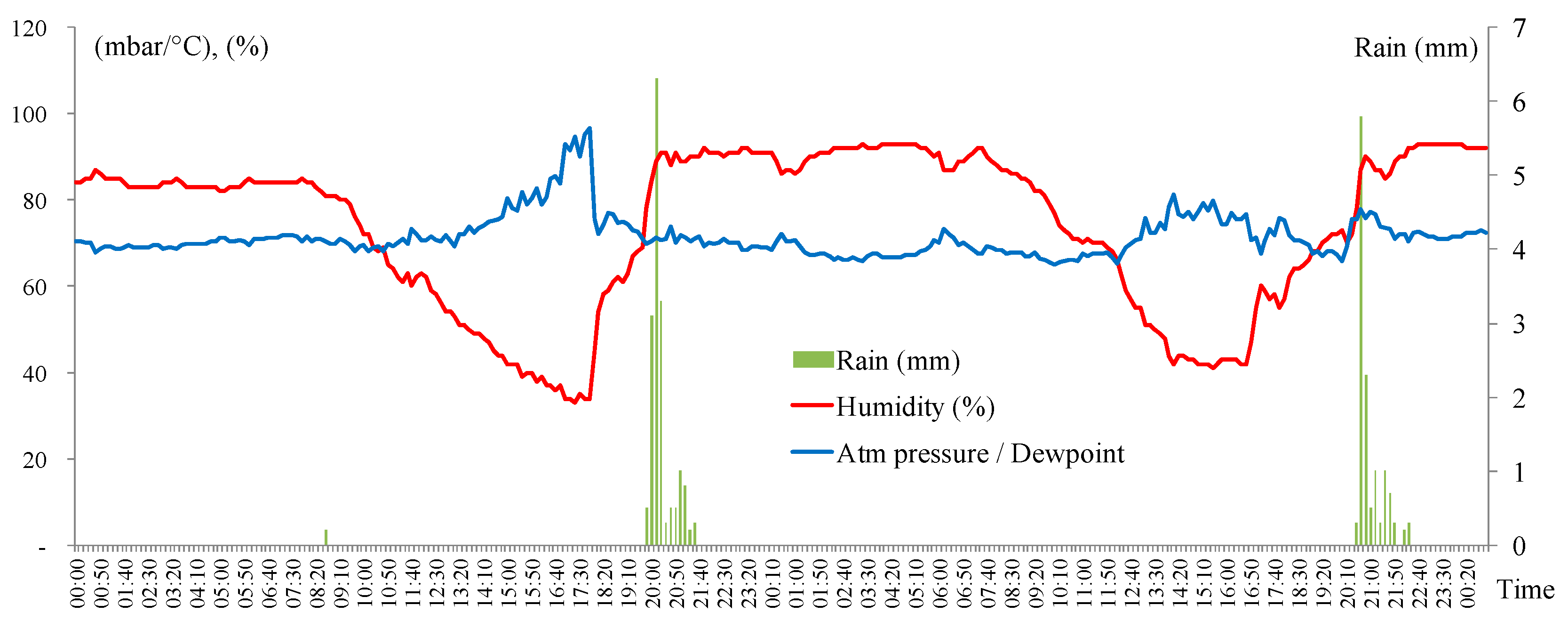
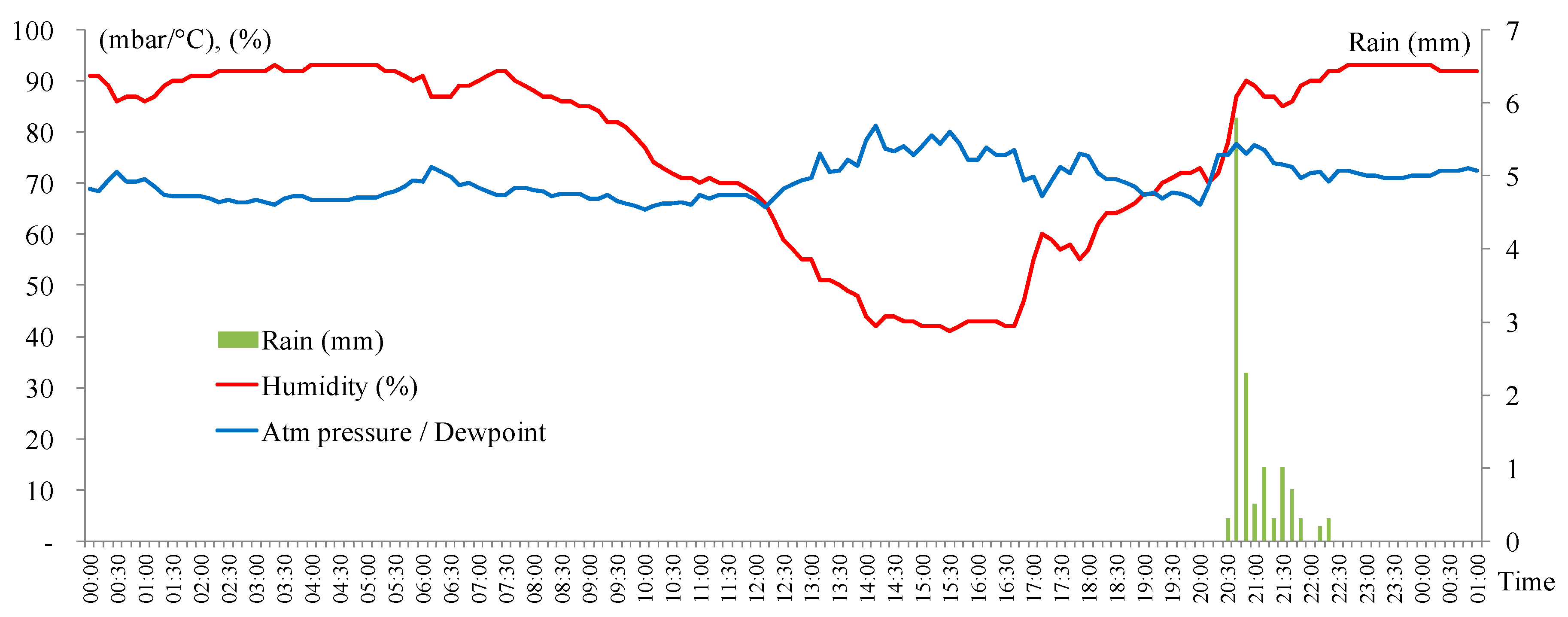
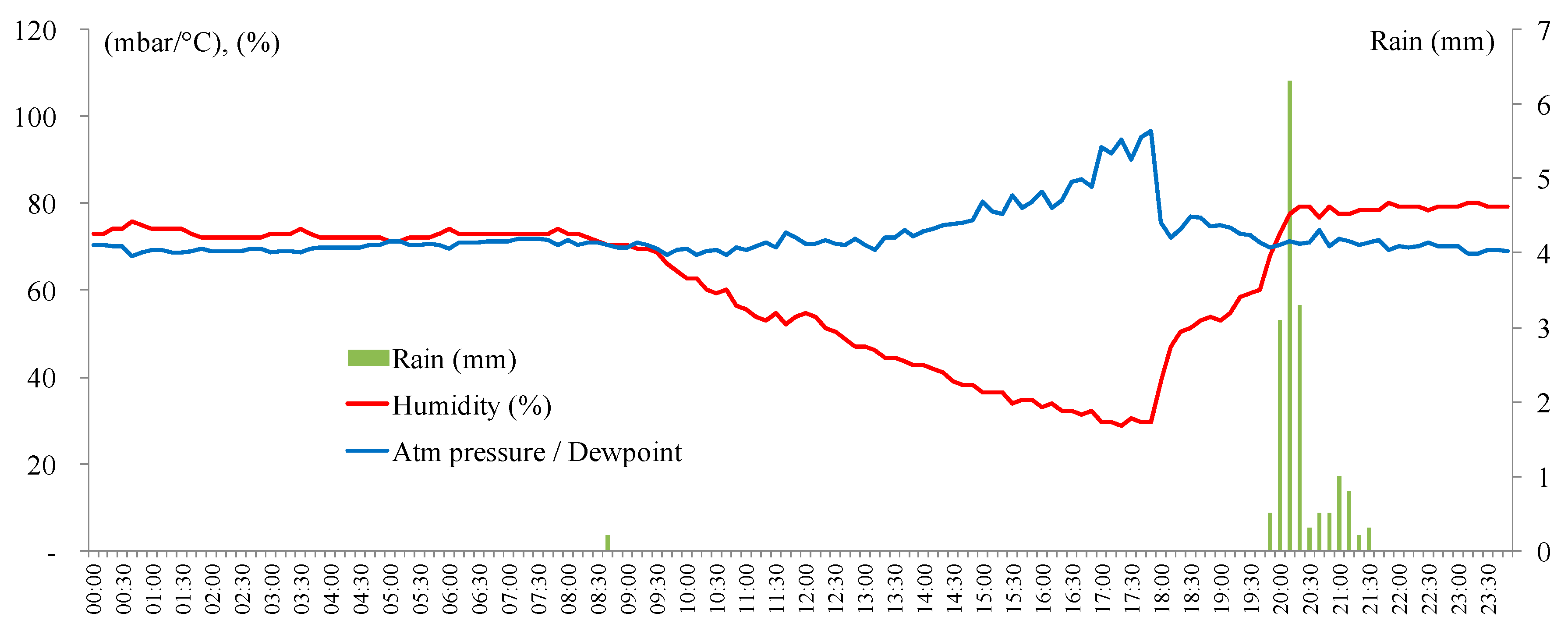
| Date | Time | Humidity (%) | Atm Pressure/Dewpoint | Rain (mm) |
|---|---|---|---|---|
| 24/06/2013 | 19:00 | 61 | 75.069 | 0 |
| 24/06/2013 | 19:10 | 63 | 74.398 | 0 |
| 24/06/2013 | 19:20 | 67 | 72.876 | 0 |
| 24/06/2013 | 19:30 | 68 | 72.679 | 0 |
| 24/06/2013 | 19:40 | 69 | 71.039 | 0 |
| 24/06/2013 | 19:50 | 78 | 69.783 | 0.5 |
| 24/06/2013 | 20:00 | 84 | 70.342 | 3.1 |
| 24/06/2013 | 20:10 | 89 | 71.287 | 6.3 |
| 24/06/2013 | 20:20 | 91 | 70.559 | 3.3 |
| 24/06/2013 | 20:30 | 91 | 71.056 | 0.3 |
| 24/06/2013 | 20:40 | 88 | 73.763 | 0.5 |
| 24/06/2013 | 20:50 | 91 | 70.110 | 0.5 |
| 24/06/2013 | 21:00 | 89 | 71.843 | 1 |
| 24/06/2013 | 21:10 | 89 | 71.365 | 0.8 |
| 24/06/2013 | 21:20 | 90 | 70.502 | 0.2 |
| 24/06/2013 | 21:30 | 90 | 70.997 | 0.3 |
| 24/06/2013 | 21:40 | 90 | 71.520 | 0 |
| State ID | Storms | EMA’s Name | |
|---|---|---|---|
| 1 | Aguascalientes | 47 | Calvillo |
| 2 | Baja California Sur | 6 | Cabo San Lucas |
| 3 | Campeche | 12 | Dzilbachen |
| 4 | Chiapas | 85 | El Triunfo |
| 5 | Chihuahua | 48 | Basaseachic |
| 6 | Coahuila | 19 | Cuatro Cienegas |
| 7 | DF | 76 | Ecoguardas |
| 8 | Edo. de Mexico | 160 | Atlacomulco, Cerro Catedral |
| 9 | Guerrero | 1 | Ciudad Altamirano |
| 10 | Hidalgo | 51 | El Chico |
| 11 | Jalisco | 18 | Chamela-Cuixmala |
| 12 | Oaxaca | 41 | Benito Juarez |
| 13 | San Luis Potosi | 35 | Ciudad Fernandez, Ciudad Valle |
| 14 | Sinaloa | 24 | El Fuerte |
| 15 | Tamaulipas | 32 | B. Del Tordo |
| 16 | Veracruz | 59 | Ciudad Aleman, Coscomatepec |
| Subtotal | 714 | ||
| 17 | Queretaro | 523 | See Appendix A, for details (34 EMA) |
| Total | 1237 |
| True | True | True | True | True |
| True | False | False | True | False |
| False | True | True | False | False |
| False | False | True | True | True |
© 2019 by the authors. Licensee MDPI, Basel, Switzerland. This article is an open access article distributed under the terms and conditions of the Creative Commons Attribution (CC BY) license (http://creativecommons.org/licenses/by/4.0/).
Share and Cite
Gutierrez-Lopez, A.; Cruz-Paz, I.; Muñoz Mandujano, M. Algorithm to Predict the Rainfall Starting Point as a Function of Atmospheric Pressure, Humidity, and Dewpoint. Climate 2019, 7, 131. https://doi.org/10.3390/cli7110131
Gutierrez-Lopez A, Cruz-Paz I, Muñoz Mandujano M. Algorithm to Predict the Rainfall Starting Point as a Function of Atmospheric Pressure, Humidity, and Dewpoint. Climate. 2019; 7(11):131. https://doi.org/10.3390/cli7110131
Chicago/Turabian StyleGutierrez-Lopez, Alfonso, Ivonne Cruz-Paz, and Martin Muñoz Mandujano. 2019. "Algorithm to Predict the Rainfall Starting Point as a Function of Atmospheric Pressure, Humidity, and Dewpoint" Climate 7, no. 11: 131. https://doi.org/10.3390/cli7110131
APA StyleGutierrez-Lopez, A., Cruz-Paz, I., & Muñoz Mandujano, M. (2019). Algorithm to Predict the Rainfall Starting Point as a Function of Atmospheric Pressure, Humidity, and Dewpoint. Climate, 7(11), 131. https://doi.org/10.3390/cli7110131