Article

Using AnnAGNPS to Simulate Runoff, Nutrient, and Sediment Loads in an Agricultural Catchment with an On-Farm Water Storage System

by
Juan D. Pérez-Gutiérrez
1,
Joel O. Paz
2,*,
Mary Love M. Tagert
2,
Lindsey M. W. Yasarer
3 and
Ronald L. Bingner
3
1
Northern Colorado Water Conservancy District, Berthoud, CO 80513, USA
2
Department of Agricultural and Biological Engineering, Mississippi State University, J. Charles Lee Building, Starkville, MS 39762, USA
3
USDA-ARS National Sedimentation Laboratory, Oxford, MS 38655, USA
*
Author to whom correspondence should be addressed.
Climate 2020, 8(11), 133; https://doi.org/10.3390/cli8110133
Submission received: 5 October 2020 / Revised: 5 November 2020 / Accepted: 10 November 2020 / Published: 12 November 2020

Abstract

:
On-farm water storage (OFWS) systems are best management practices that consist of a tailwater recovery (TWR) ditch used with a storage pond to provide irrigation water and improve downstream water quality. These systems have been increasingly implemented in the southeastern US, but the individual and cumulative effects of these systems on a watershed scale are unknown. In this study, the runoff, nutrient, and sediment loads entering a TWR ditch in an agricultural catchment were quantified, and contributing sources were identified using the annualized agricultural non-point source (AnnAGNPS) model. Fields with larger areas and soils with a high runoff potential produced more runoff. The volume of runoff exceeded the TWR ditch storage volume approximately 110 times, mostly during the winter and spring seasons. During years when corn and winter wheat were planted, NO3–N loads increased because these crops need nitrogen fertilization to grow. Planting winter wheat in priority subwatersheds reduced the total phosphorous (TP) and sediment loads by about 19% and 13%, respectively, at the TWR ditch inlet. Planting winter wheat can reduce runoff, TP, and sediment loads but also result in higher NO3–N loads. AnnAGNPS simulations quantified the benefits of an OFWS system to advance the understanding of their impact on water availability and quality at a watershed scale.

1. Introduction

The global population has been projected to increase between 9.6 billion and 12.3 billion by 2100 [1]. As a result, agriculture will have to double its productivity to feed people [2,3]. Meeting this increasing food demand has led to the intensification of agriculture, which translates into the greater use of chemical inputs and pressure on soil and water resources. Agricultural activities often transfer excess fertilizers through non-point source (NPS) pollution into aquatic ecosystems causing devastating ecological and economical effects [4,5,6,7,8]. Therefore, a balance between increasing yields and mitigating adverse environmental impacts is crucial for the future of agriculture.
The implementation of best management practices (BMPs) has been recognized to significantly reduce NPS pollution from croplands to downstream waterbodies [9,10,11]. However, much effort is still devoted to quantifying the effectiveness and benefits of such practices, especially newer BMPs. Measuring BMP performance can be a challenge because their benefits vary spatially and temporally due to the heterogeneity of the landscape and seasonality of hydrological factors [12]. The challenge is even greater when attempting to evaluate the effects of several BMPs combined [13,14,15], address the shift in BMP performance over time [16], and understand lag times in water quality response [17]. The use of watershed models can be a feasible alternative to quantify the effectiveness of BMPs while accounting for these challenges [16,18,19,20,21,22,23,24]. However, due to the diversity of BMPs that can be implemented over agricultural fields, information describing the performance of each BMP and the combined use of different BMPs is limited.
Structural BMPs such as tail-water recovery (TWR) ditches and agricultural ponds (i.e., on-farm water storage systems—OFWS) can improve downstream water quality by significantly reducing nutrient loads from agricultural watersheds [25,26,27]. The dual benefit of reducing nutrient pollution and supplying water for irrigation is important in areas such as the Lower Mississippi River Valley, where agricultural production strongly depends on irrigation. Farmers and landowners in this region are tasked with (1) reducing off-site movement of nutrients, which contributes to the hypoxic zone in the northern Gulf of Mexico, and (2) conserving water resources to slow the declining groundwater levels in the Mississippi River Valley Alluvial Aquifer (MRVAA), the primary source of water for irrigation. Consequently, OFWS systems have been implemented across the MRVAA, especially in areas with more severe groundwater declines. Although research has highlighted in-ditch and in-pond nutrient reductions, less attention has been placed on estimating the water and nutrient loads entering and exiting OFWS systems [28,29]. Evaluating the OFWS drainage area will quantify the impacts of these systems on a watershed scale, which will advance our understanding of the cumulative effects of these systems on water quality and groundwater decline as more OFWS systems are implemented throughout a watershed.
The annualized agricultural non-point source (AnnAGNPS) model [30,31] is a watershed model that has been designed to measure the impact of agricultural management practices on hydrological and water quality responses in watersheds. Most studies using the AnnAGNPS model demonstrate its performance after model calibration with field-observed data [22,32,33,34,35,36,37,38,39]. However, AnnAGNPS has also been used for similar purposes without conducting calibration with measured data. A study used the model with no calibrated parameters to estimate the runoff and sediment in an agricultural watershed within the Mississippi Delta Region [21]. They concluded that the model had an adequate ability to simulate monthly and annual runoff and sediment yield with no calibration process. This finding is of significant interest because it is difficult and costly to secure sufficient observed data to conduct calibration processes in watershed-scale modeling studies. To date, efforts to assess the benefits of tail-water recovery ditches using watershed scale models has been limited. This is, at least in part, because these ditches have multiple inlets. Therefore, the collection of measured runoff and water quality data (and especially continuous measured runoff and water quality data) is usually impractical and expensive, making it a challenge to collect a sufficient quantity of measured data on even one OFWS system. However, estimating the effects of OFWS systems at various scales is critical to stakeholders and agencies to better identify where these systems can be implemented to improve water quality and relieve pumping pressure on groundwater.
In this study, the AnnAGNPS model was used without calibration with field data to simulate runoff, sediment, and nutrient loads and identify the main contributing areas draining to a TWR ditch established as part of an OFWS system within Porter Bayou Watershed, Mississippi. The quantification of the water, nutrient, and sediment loading is an essential step in understanding the water quality and quantity benefits of OFWS systems when implemented in agricultural watersheds, as well as how the management of these systems might be altered to improve performance. Predictions on the volume of water captured by OFWS systems can also help determine their potential for alleviating local flooding. Finally, this study advances the incorporation of an OFWS system and the associated watershed impacts into the AnnAGNPS model, with the goal of improving the ability of AnnAGNPS to model these systems on a larger scale.

2. Materials and Methods
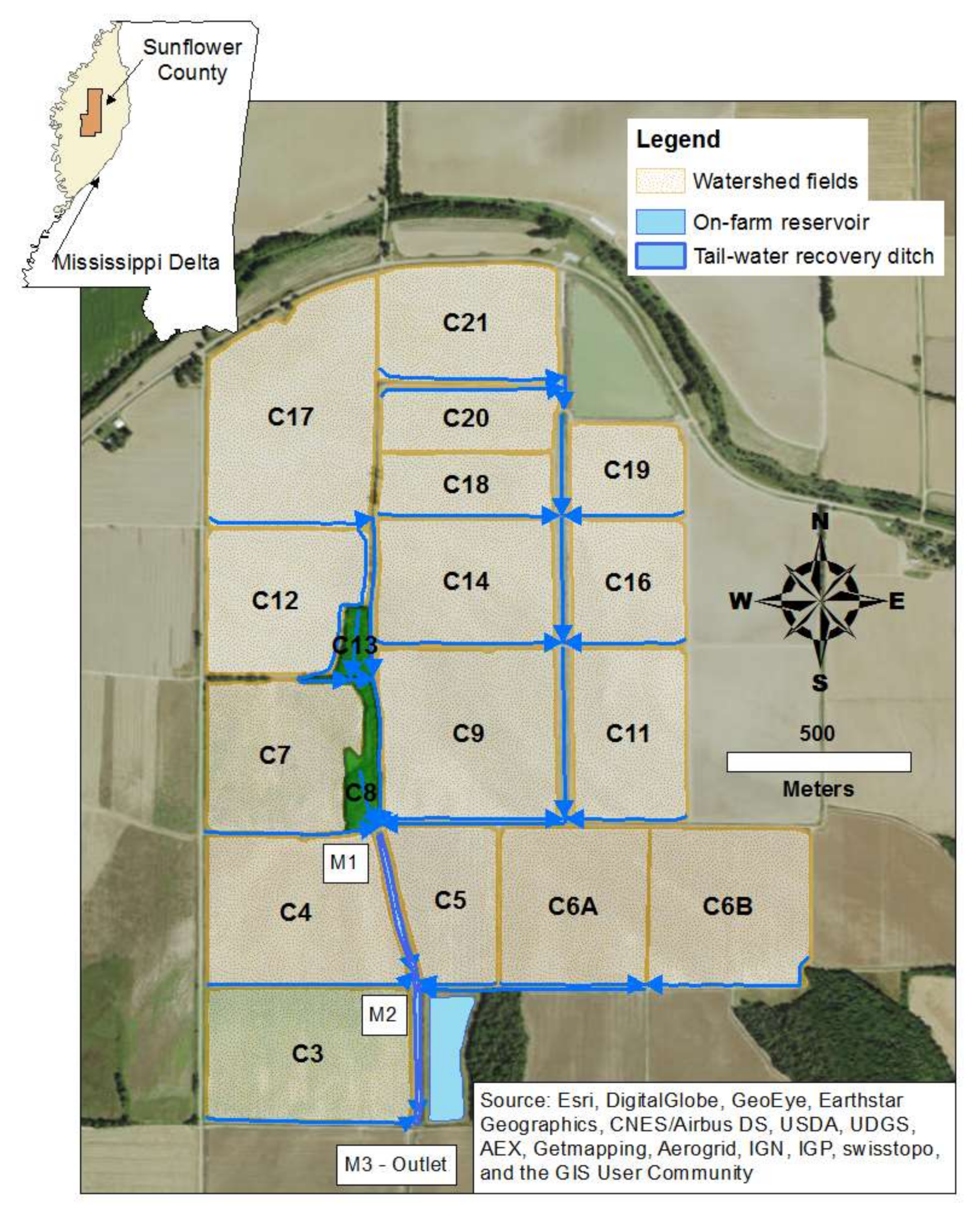
2.1. Study Site

This investigation was conducted in the Porter Bayou Watershed (PBW; 33°26′39″–33°51′38″ N, 90°48′54″–90°31′34″ W) in the Mississippi Delta Region (MDR), an intensively farmed area located in northwest Mississippi, USA (Figure 1). For the AnnAGNPS simulation, a small 214 ha watershed within the PBW located north of Indianola, MS, in Sunflower county, was selected, and it included Metcalf farm and the surrounding area that drains into the OFWS system outlet at M3 (Figure 1). The major crops grown from 2012 to 2016 were soybeans, corn, and rice (Table 1). Winter wheat was planted during 2013 and 2014 in four and two fields, respectively. The watershed is dominated by the following soil types: Forestdale, Tensas, Dundee, Pearson, and Dowling, which are primarily poorly drained soils and prone to produce high runoff. In addition, the watershed is relatively flat with surface elevations ranging from 130 to 135 m. The average temperature ranged from −8.3 °C in winter 2014 to 32.2 °C in summer 2012 (Figure 2a). The lowest total seasonal precipitation was 99 mm observed in summer 2015, while the highest was 579 mm in spring 2014 (Figure 2b). Average annual precipitation was 1308 mm, and in 2013 and 2014 this average was exceeded by 242 mm and 114 mm, respectively. Meanwhile, 2012 and 2015 were drier years with a total annual rainfall of 1100 and 1133 mm, respectively.
The OFWS system consists of a trapezoidal-shape TWR ditch and an elongated agricultural pond which have a combined storage volume of 128,020 m3 (TWR ditch: 13,320 m3; pond: 114,700 m3). Water flows from north to south through the ditch, which is 818.8 m long and 1.8 m deep on average; the pond is 2.4 m deep with a surface area of 4.45 ha. Runoff is routed to the single outlet pipe (33°39′35.6″ N, 90°39′11.9″ W) set at 1.2 m above the canal bed (Figure 1). The system was designed according to National Resources Conservation Service (NRCS) [40] guidelines, and more information about its characteristics can be found at Pérez-Gutiérrez, Paz and Tagert [25].

2.2. Model Description

AnnAGNPS is a physical process model developed to simulate the runoff, sediment, nutrient, and pesticide yields at a daily time step in small watersheds. The model divides the watershed into subwatersheds based on homogeneous physical characteristics such as soil type, land use, and land management. AnnAGNPS is a continuous simulation model and has been primarily developed to evaluate the impacts of different agricultural management practices on watersheds. As with other physical process watershed-scale models, the major input data are climate, land characterization, field operations, chemical characteristics, and feedlot operations. A detailed description of the model can be found in Geter and Theurer [30], Bingner, et al. [41], Bosch, et al. [42], Theurer and Cronshey [43], Cronshey and Theurer [44].

2.3. Model Input

A detailed field survey was conducted to identify the field boundaries and collect elevation data required by the model. Eighteen fields were identified as subwatersheds (or cells), and associated reaches were defined for routing runoff to the outlet (M3) in the AnnAGNPS model (Figure 1). Because all fields were precision leveled, they were defined as homogeneous drainage areas or subwatersheds. The delineation of the watershed was done manually with the aid of GoogleTM Earth and geographic information system (GIS) technologies. Parameters describing the subwatersheds such as area, average elevation, and average land slope were determined from the field survey (Table 1). Parameters representing the time of concentration and travel time were computed from data provided by the field reconnaissance following USDA-SCS [45] methods, modified by Theurer and Cronshey [43]. Soil data and physical properties were obtained from the Soil Survey Geographic (SSURGO) database [46]. Although 15 soil types were identified throughout the watershed, the dominant soil type was determined for each subwatershed as required by the model, using GIS operations (Table 1). Crop planting dates were obtained from the Sunflower county USDA–NRCS office. A crop management schedule was assigned to each field according to the typical management practices conducted in the MDR (Table 2). Irrigation was included in the crop management schedule, starting in late May or June and ending in August. The SCS curve number is an important model parameter used to estimate runoff. Table 3 shows the curve numbers used in the model, based on different land use categories and hydrologic soil types in the watershed. Weather data were recorded automatically at 15-min intervals from March 2012 to December 2016 by a WatchDog 2700 Weather Station (Spectrum® Technologies, Inc., Aurora, IL) located 9.2 km southeast of the outlet (M3). The weather data were subsequently processed to create daily time scale files as required by the AnnAGNPS model. Data from the Parameter-elevation Regressions on Independent Slopes Model (PRISM) Climate Group (http://www.prism.oregonstate.edu/explorer/) were used to fill any gaps in rainfall records. Other missing weather data such as daily maximum and minimum temperature, dew point, wind velocity, and solar radiation were patched using data from the Moorhead, MS climate station, which is located 22 km south of the study site and managed by the National Oceanic and Atmospheric Administration.
AnnAGNPS was used to simulate the runoff, sediment, and nutrient loads entering the TWR ditch. The model was set to run for two initialization years (2010–2011) to establish antecedent conditions before beginning the simulation period over the next five years (2012–2016). As described by Bosch, Theurer, Bingner, Felton and Chaubey [42], AnnAGNPS outputs are predefined by the user for the watershed source of interest (subwatersheds, reaches, among others). The model produces event-based output as well as monthly and annual summaries of hydrologic and water quality parameters. The model partitions nitrogen and phosphorus load into sediment-bound and dissolved fractions. This study used dissolved nitrate nitrogen (NO3–N) and total phosphorus (TP) to represent NO3–N and TP, respectively, and employed AnnAGNPS to estimate the runoff, sediment, NO3–N, and TP loads entering a TWR ditch.

3. Results and Discussion

Table 4 presents the average annual runoff, nutrient and sediment loads entering the TWR ditch per unit area, as well as the contributing fields and total area draining to each point—M1, M2, or main outlet M3—in the TWR ditch. The load values represent the aggregate contributions divided by the area of the fields draining into the TWR ditch at each outlet. These values provide a unique picture of the impact of each source area regardless of size. Annual runoff volume per unit area entering the ditch at mid-point M2 was slightly higher than the runoff entering at the M1 or M3 by about 600 m3 ha−1 yr−1, even though M2 had the smallest drainage area. This difference is attributed to the runoff potential of the fields draining to M2. Subwatershed C4 is the field covering the third largest area of all subwatersheds, and soil in this field has the highest runoff potential (hydrologic soil group D). In addition, reaches transporting runoff flow directly into the ditch from subwatersheds C4 and C5. This direct flow path minimizes the amount of water allowed to infiltrate or evaporate and results in a greater volume of water draining into the ditch.
The NO3–N load per unit area was higher at M1 as most of the fields that were planted with corn and winter wheat during the simulation period are located upstream of M1. The TP load entering the ditch at M3 tended to be higher. Subwatershed C3, one of the three fields that drained to M3, was the only field that was simulated as a turn area. Typically, turn areas have compacted soils and do not have vegetation. This means that the soil in this field is highly susceptible to erosion and the off-site movement of nutrients by rainfall–runoff, which might explain the higher TP load simulated by AnnAGNPS at M3. Sediment loading did not show much variation through the TWR ditch segments, indicating that the sediment load might be equally distributed over the total area contributing to the TWR ditch outlets.

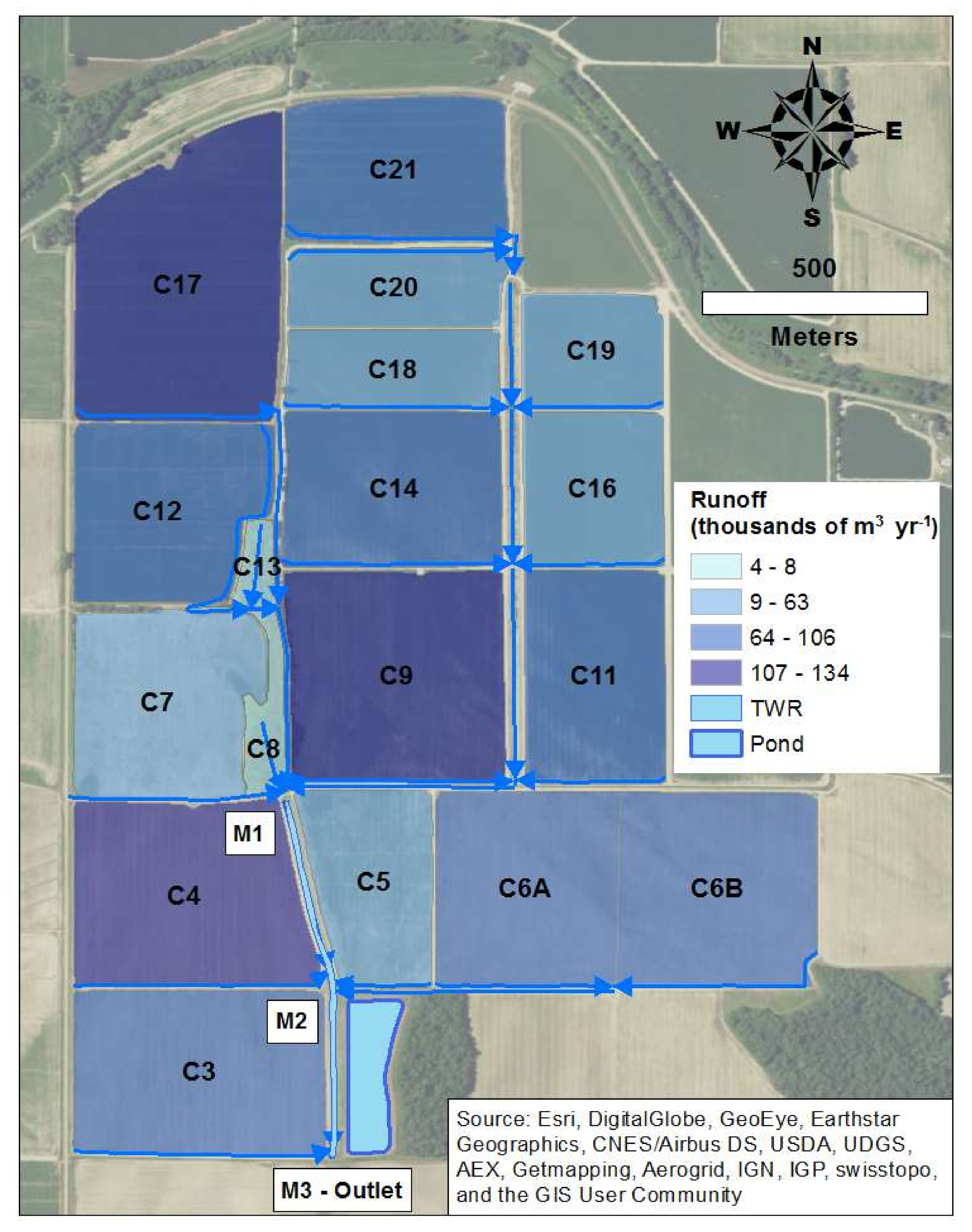
3.1. Spatial Variation

The average annual runoff estimated by the AnnAGNPS model is shown in Figure 3. During the 5-year simulation period (2012–2016), the model estimated an average annual runoff of 1,370,053 m3 that drained into the main outlet at M3, of which 11% was contributed by irrigation runoff. The five highest runoff-producing subwatersheds were C17 (9.73%), C9 (9.31%), C4 (8.78%), C6B (7.74%), and C3 (7.47%). These five fields cover a large drainage area (a combined 90.83 ha out of the total area of 214.04 ha) when compared to other fields in the watershed, which may explain the high runoff production. NO3–N load transported throughout the watershed to M3 resulted in 623.2 kg yr−1 (Figure 4). Five subwatersheds contributed 56.2% of the average annual NO3–N load, and the order was: C17 (18.41%) > C21 (16.15%) > C11 (8.29%) > C16 (7.03%) > C6A (6.36%). The average annual TP load from 2012 to 2016 in each subwatershed is shown in Figure 5, and the average annual TP load for the whole watershed resulted in 256 kg yr−1. Five subwatersheds contributed 66.2% of the average annual TP load in the following order: C9 (21.7%) > C3 (18.66%) > C17 (16.16%) > C6A (5.09%) > C21 (4.06%). The average annual sediment load resulted in 312.8 tons yr−1, and five subwatersheds contributed 62% of the average annual sediment load (Figure 6) in the following order: C17 (36.18%) > C6B (7.47%) > C5 (6.45%) > C11 (6.03%) > C21 (5.84%). A list of seven subwatersheds that had the greatest impact on water quantity and quality in the simulated watershed is shown in Table 5. Five subwatersheds (C17, C6B, C21, C9, and C3) were designated as priority subwatersheds because they ranked at least first or second with respect to runoff production, NO3–N load, TP load, or sediment load. Subwatershed C17, which has the largest area (22.54 ha) and the second highest average slope (0.0019), generated the highest sediment and NO3–N loads. Soils in this field, classified as a hydrologic soil group C, are shallow and have below-average infiltration, and thus have moderately high runoff potential. Furthermore, crops in this field were more diverse and varied between rice, corn, soybean, and winter wheat with assigned curve numbers ranging from 83 to 90. Higher curve numbers translate into higher runoff, and this effect is magnified over larger fields when rainfall occurs. Runoff transported higher loads of nitrogen when corn and winter wheat were planted because these crops required 150 kg ha−1 and 120 kg ha−1 of soluble nitrogen fertilizer, respectively. However, winter wheat might have reduced TP load during winter. Therefore, the combined effect of landscape characteristics and fertilizer application played a more influential role in the nutrient load from the C17 subwatershed. Subwatershed C9 has an area of 18.70 ha (ranked second in size) and soils classified as hydrologic soil group D. The C9 subwatershed produced the largest TP load of all subwatersheds and ranked second in terms of runoff volume. This subwatershed was planted in a soybean–rice rotation for four years and then planted with corn, which was fertilized with 150 kg ha−1 of soluble nitrogen and 13 kg ha−1 of phosphorus in 2016. Thus, the area of the subwatershed seemed to be an important factor for the TP load contribution in the watershed.
Subwatershed C6B was ranked fifth and third with respect to the magnitude of the area and average land slope, respectively, and was classified as having soils in hydrologic soil group D. The C6B subwatershed generated the second highest sediment load of all subwatersheds and was planted primarily with soybeans except during 2013, when corn was planted. In addition, the C3 subwatershed ranked fourth in magnitude of area and ninth with respect to the average land slope and generated the second highest TP load of all subwatersheds. The C3 subwatershed had soils classified as hydrologic soil group D and was simulated as a turn area, which explained the high TP load attached to sediments and transported by runoff. Finally, the subwatershed C21 also had soils in hydrologic soil group D and was ranked tenth in areal extent and seventh for average land slope. The C21 subwatershed produced the second highest NO3–N load of all subwatersheds. Similar to C17, subwatershed C21 was also planted with corn and winter wheat during two consecutive years in 2013 and 2014.

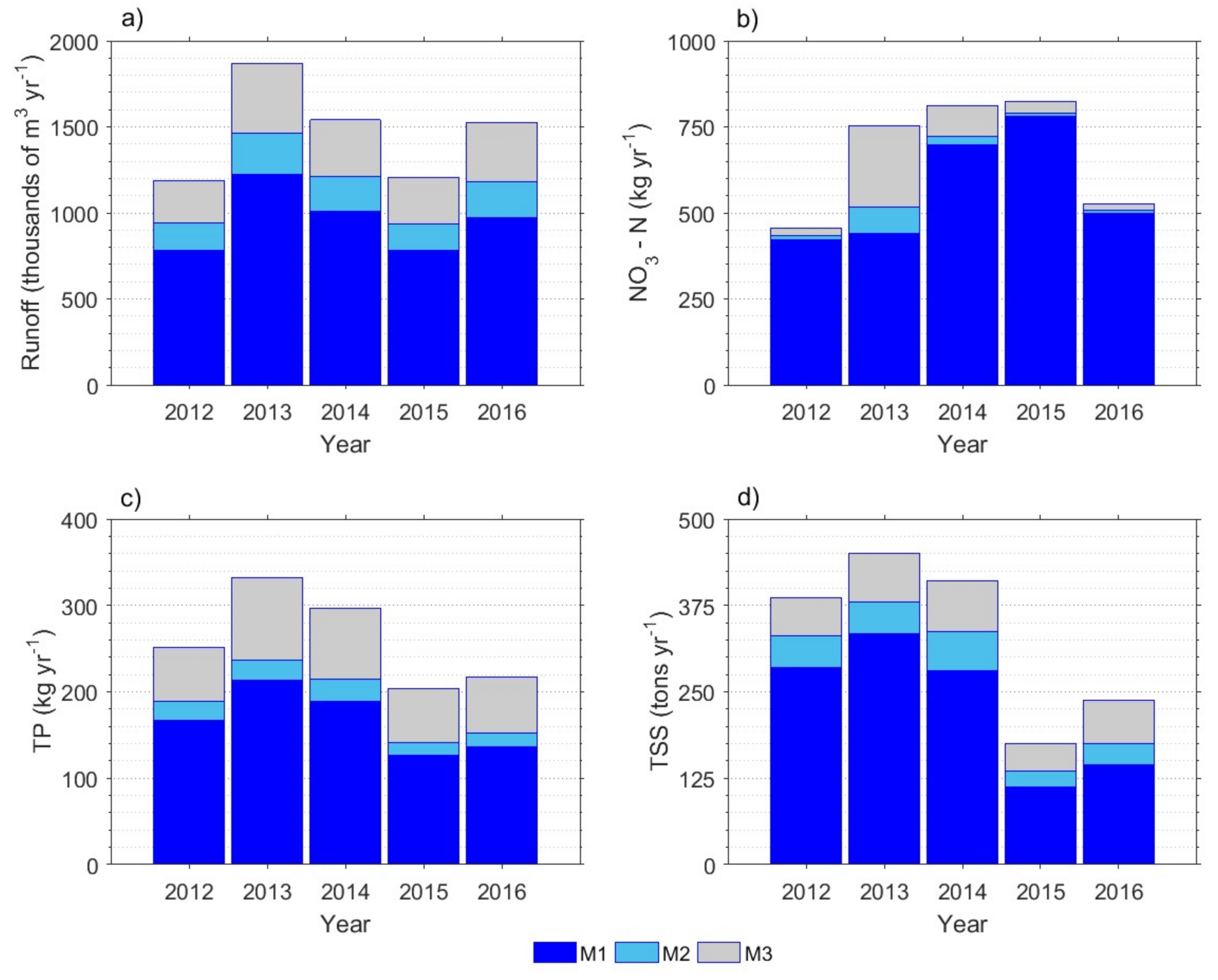
3.2. Temporal Variation

The total annual runoff production and nutrient and sediment load from the simulated watershed, as estimated by the AnnAGNPS model, are shown in Figure 7. During the 5-year simulation period (2012–2016), an average annual total runoff of 1,465,678 m3 drained to the main outlet at M3. This volume exceeds the TWR ditch storage volume by roughly 110 times, which highlights the magnitude of surface water available in the simulated watershed. In terms of runoff produced by year, the order was 2013 > 2014 > 2016 > 2015 > 2012 (Figure 7a), which followed the same pattern for total precipitation by year. Overall, fields draining upstream from the TWR ditch to the inlet at M1 generated the highest volume of runoff at a rate of 952,578 m3 yr−1, which resulted in roughly 65% of the total runoff volume produced annually. Fields draining into the TWR ditch between M1 and M2 contributed 13.3% of the annual runoff production, and fields draining into the ditch between M2 and M3 contributed 21.7% of the average annual runoff.
The changes in total annual NO3–N load for each TWR ditch segment are shown in Figure 7b. Nitrate nitrogen was highest in 2015, followed in order of magnitude by 2014, 2013, 2016, and 2012. Overall, the area that drained into M1 was responsible for the greatest percentage of the NO3–N load in the TWR ditch in all years. During the 2013 growing season, 41.4% of the watershed was planted with corn, mainly in five (C17, C6B, C21, C6A, C5) of the highest runoff contributing fields in the simulated watershed (Table 5). Winter wheat covered 12.2% of the watershed after the summer growing season in 2013. Both corn and winter wheat were fertilized with soluble nitrogen, which is reflected by the high NO3–N load that was simulated by the model in 2013. In 2014, rainfall was highest during spring, roughly equally distributed between summer and fall, and minimal in winter. In fall 2014, the subwatersheds with the highest contributing nitrate loads, C17 and C21, were planted with winter wheat, which was fertilized with soluble nitrogen. Available nitrogen in soil after the fertilizer application was likely transported by runoff from the 2014 winter and 2015 spring rainfall, which might explain the higher NO3–N load during these years. In addition, soybeans were planted on 84% of the simulated watershed during 2014. After soybeans were harvested, 33% of the nitrogen that was used by the plant was left over in the soil [48], available for potential transformation mediated by microorganisms and susceptible to movement off fields by runoff.
Total annual sediment and TP loads were highest in 2013, followed in order of magnitude by 2014, 2012, 2016, and 2015 (Figure 7c,d). The changes in TP and sediment loads were similar and can be attributed to the fact that phosphorus is usually transported as sediment-bound phosphorus. Similar to the pattern observed for NO3–N, the bulk of TP and sediment were from the area that drains into M1. In addition, TP and sediment loads entering the ditch between M2 and M3 were generally higher than the loads entering the system between M1 and M2. In 2013, significant amounts of precipitation were recorded in winter, fall, and spring. These conditions favored the production of runoff from fields with exposed soil, and it is highly likely that erosion due to high runoff resulted in greater loads of TP and sediment in 2013. In contrast, the NO3–N load during 2014 was higher than during 2013. One possible explanation is that most of the fertilizer applied during spring and fall of 2014 was transported off the field as most of the rain fell during these two seasons. In addition, during 2013 and 2014, 41.5% of the simulated watershed was planted with corn and 16.6% with winter wheat. Planting winter wheat after corn seemed to result in larger NO3–N loads transported with runoff. Rainfall was higher during the winter and summer of 2016 and minimal during spring and fall. In 2016, the fields were planted with corn (34.7%), soybean (26.5%), and rice (22.7%). Runoff produced in 2012 and 2015 was the lowest among the 5-year simulation period, which may be attributed to less rainfall observed in 2012 and 2015 as compared to other years. The water savings potential of the TWR ditch was estimated by combining the simulated runoff and discharge water measured at the ditch outlet available for 2016 (Figure 8). Of the 1,526,105 m3 of runoff produced, 56.5% (862,581 m3) was saved by the ditch in 2016.

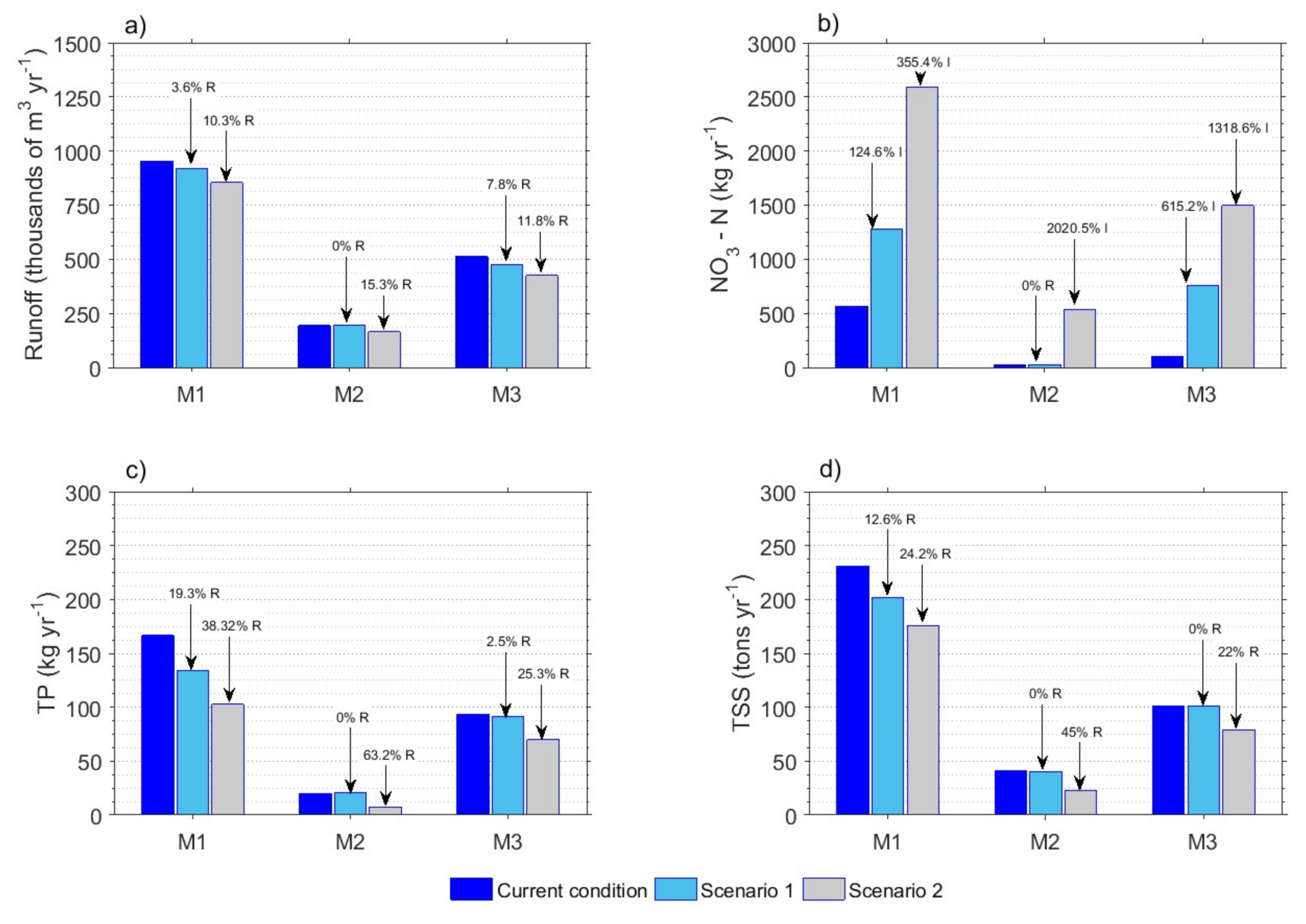
3.3. Impact of Additional Agricultural Management Operations

To examine the impacts of management practices on water quality and quantity, two scenarios were implemented in AnnAGNPS. Scenario 1 planted winter wheat in priority subwatersheds (C17, C6B, C21, C9, and C3), and Scenario 2 planted winter wheat in all subwatersheds. With more rainfall occurring outside the summer growing season, winter wheat could be an option for producers unable to irrigate or those trying to use less water for irrigation. The current management practices were set as the baseline scenario. The impacts of Scenarios 1 and 2 on the estimated average annual runoff, sediment, and nutrient loads at different locations within the TWR ditch (M1, M2, and M3) are shown in Figure 9. The targeted implementation of management practices (Scenario 1) reduced the TP and sediment loads at M1 by 19.3% and 12.6%, respectively. However, under Scenario 1, NO3–N loading increased substantially at all locations primarily because winter wheat was fertilized with soluble nitrogen at a rate of 120 kg ha−1. This suggests that some of the nitrogen applied to fields may have been transported off-site by runoff.
Scenario 2 resulted in greater average annual reductions of TP and sediment loads than Scenario 1. If winter wheat is planted in all subwatersheds, TP loads from the areas upstream of M1 are predicted to decrease by approximately 38% from the current conditions. Reductions in TP loads at M2 and M3 were about 63% and 25%, respectively. Reductions in sediment loads followed a similar pattern as those for TP, with a higher percentage reduction at the upstream outlet locations—M1 (24.2%) and M2 (45%)—than at the downstream outlet—M3 (22%). The all winter wheat scenario also showed a reduction in runoff. In total, 188,100 m3 (97,900 m3 at M1; 29,700 m3 at M2; and 60,500 m3 at M3) of runoff were reduced from the fields draining to the TWR ditch. Despite the positive effects that could result from planting winter wheat in the target watershed, AnnAGNPS simulations showed very high increases in the NO3–N load entering the ditch at M1 due to the nitrogen fertilization necessary to grow winter wheat. Conservationists and policy makers should be mindful that implementing management practices to improve water quality might have positive effects on one variable but associated undesirable tradeoffs on another variable (Smith et al., 2019). Although cover crops may reduce NO3–N leaching to groundwater, the NO3–N load may increase with runoff due to biomass leaching during rainfall events [49]. This effect might be exacerbated if soluble nitrogen is applied over poorly drained soils with a high runoff potential.

4. Summary and Conclusions

The AnnANGPS model was used to estimate the water, sediment, and nutrient loads entering a TWR ditch implemented as part of an OFWS system in an agricultural watershed within the PBW, Mississippi. Simulations showed that the fields with larger areas that have soils with a high runoff potential (hydrologic soil group C or D) resulted in higher runoff, and this condition mirrored annual rainfall patterns. The volume of runoff exceeded the TWR ditch storage volume by roughly 110 times, mostly during the winter and spring seasons. Therefore, these seasons offer the highest potential for capturing excess water in the OFWS system. Results showed that the fields with larger areas also produced the highest total nutrient and sediment loads. AnnAGNPS simulations showed that NO3–N loads were sensitive to fertilizer application. Therefore, during years when corn and winter wheat were planted and fertilized, NO3–N loading increased. The TP and sediment loading patterns were similar and were influenced by the hydrological temporal conditions.
Assessment of different management scenarios indicated that planting winter wheat can benefit water quality by reducing sediment loads and the export of TP. However, winter wheat requires nitrogen fertilizer, which can result in higher NO3–N loads washed off by runoff. In particular, if winter wheat is planted in the priority subwatersheds (Scenario 1), TP and sediment loads are reduced by about 19% and 13%, respectively, at M1. Although planting winter wheat in all fields (Scenario 2) may not be feasible, this scenario would substantially reduce TP and sediment loads from the contributing areas draining to M1 (TP: 3%; sediment: 24%) and M2 (TP: 63%; sediment: 45%) in the TWR ditch. Scenario 2 also showed that 188,100 m3 of runoff can be reduced from fields draining to the TWR ditch.
Results of this study provide both stakeholders and agencies with critical information needed to better identify where these systems can be implemented to improve water quality and relieve pumping pressure on groundwater in the Lower Mississippi River Alluvial Valley. In addition, this study suggests that agricultural watersheds in the MDR might produce substantial amounts of runoff, which could be an important source of water for irrigation if properly managed. While managing the water availability during winter and spring, nutrient reduction benefits of OFWS systems can be maximized.

Author Contributions

Conceptualization, J.D.P.-G., J.O.P., M.L.M.T., L.M.W.Y., R.L.B.; methodology, J.D.P.-G., J.O.P., M.L.M.T., L.M.W.Y., R.L.B.; software, J.D.P.-G., L.M.W.Y., R.L.B.; formal analysis, J.D.P.-G., J.O.P., M.L.M.T., L.M.W.Y., R.L.B.; investigation, J.D.P.-G., J.O.P., M.L.M.T., L.M.W.Y., R.L.B.; resources, J.D.P.-G., J.O.P., M.L.M.T., R.L.B.; data curation, J.D.P.-G., L.M.W.Y., R.L.B.; writing—original draft preparation, J.D.P.-G.; writing—review and editing, J.D.P.-G., J.O.P., M.L.M.T., L.M.W.Y., R.L.B.; visualization, J.D.P.-G.; supervision, J.O.P., M.L.M.T.; project administration, J.O.P., M.L.M.T.; funding acquisition, J.O.P., M.L.M.T. All authors have read and agreed to the published version of the manuscript.

Funding

USDA NIFA funded this project under the National Integrated Water Quality Program (Grant # 2011-51130-31168).

Acknowledgments

We would like to express our gratitude to Trinity Long from USDA–NRCS for providing information about agricultural practices applied in the Mississippi Delta Region. We also thank Boyer Britt for allowing us to work in his field.

Conflicts of Interest

The authors declare no conflict of interest. This work does not reflect official Northern Colorado Water Conservancy District’s policy.

References

  1. Gerland, P.; Raftery, A.E.; Ševčíková, H.; Li, N.; Gu, D.; Spoorenberg, T.; Alkema, L.; Fosdick, B.K.; Chunn, J.; Lalic, N. World population stabilization unlikely this century. Science 2014, 346, 234–237. [Google Scholar] [CrossRef] [Green Version]
  2. Tilman, D.; Cassman, K.G.; Matson, P.A.; Naylor, R.; Polasky, S. Agricultural sustainability and intensive production practices. Nature 2002, 418, 671–677. [Google Scholar] [CrossRef] [PubMed]
  3. Tilman, D.; Balzer, C.; Hill, J.; Befort, B.L. Global food demand and the sustainable intensification of agriculture. Proc. Natl. Acad. Sci. USA 2011, 108, 20260–20264. [Google Scholar] [CrossRef] [Green Version]
  4. Ladapo, H.; Aminu, F. Agriculture and eutrophication of freshwaters: A review of control measures. J. Res. For. Wildl. Environ. 2017, 9, 67–74. [Google Scholar]
  5. Withers, P.; Neal, C.; Jarvie, H.; Doody, D. Agriculture and eutrophication: Where do we go from here? Sustainability 2014, 6, 5853. [Google Scholar] [CrossRef] [Green Version]
  6. Rabotyagov, S.; Kling, C.; Gassman, P.; Rabalais, N.; Turner, R. The economics of dead zones: Causes, impacts, policy challenges, and a model of the Gulf of Mexico hypoxic zone. Rev. Environ. Econ. Policy 2014, 8, ret024. [Google Scholar] [CrossRef] [Green Version]
  7. Rabalais, N.N.; Turner, R.E.; Scavia, D. Beyond science into policy: Gulf of Mexico hypoxia and the Mississippi River nutrient policy development for the Mississippi River watershed reflects the accumulated scientific evidence that the increase in nitrogen loading is the primary factor in the worsening of hypoxia in the northern gulf of mexico. BioScience 2002, 52, 129–142. [Google Scholar]
  8. Carpenter, S.R.; Stanley, E.H.; Vander Zanden, M.J. State of the world’s freshwater ecosystems: Physical, chemical, and biological changes. Annu. Rev. Environ. Resour. 2011, 36, 75–99. [Google Scholar] [CrossRef] [Green Version]
  9. Osmond, D.L. USDA water quality projects and the National Institute of Food and Agriculture Conservation Effects Assessment Project watershed studies. J. Soil Water Conserv. 2010, 65, 142A–146A. [Google Scholar] [CrossRef] [Green Version]
  10. Tomer, M.; Sadler, E.; Lizotte, R.; Bryant, R.; Potter, T.; Moore, M.; Veith, T.; Baffaut, C.; Locke, M.; Walbridge, M. A decade of conservation effects assessment research by the USDA Agricultural Research Service: Progress overview and future outlook. J. Soil Water Conserv. 2014, 69, 365–373. [Google Scholar] [CrossRef] [Green Version]
  11. Tomer, M.; Locke, M. The challenge of documenting water quality benefits of conservation practices: A review of USDA-ARS’s Conservation Effects Assessment Project watershed studies. Water Sci. Technol. 2011, 64, 300–310. [Google Scholar] [CrossRef] [PubMed]
  12. Her, Y.; Chaubey, I.; Frankenberger, J.; Jeong, J. Implications of spatial and temporal variations in effects of conservation practices on water management strategies. Agric. Water Manag. 2017, 180, 252–266. [Google Scholar] [CrossRef]
  13. Meals, D.W. Detecting changes in water quality in the Laplatte River watershed following implementation of BMPs. Lake Reserv. Manag. 1987, 3, 185–194. [Google Scholar] [CrossRef]
  14. Arabi, M.; Frankenberger, J.R.; Engel, B.A.; Arnold, J.G. Representation of agricultural conservation practices with SWAT. Hydrol. Process. 2008, 22, 3042–3055. [Google Scholar] [CrossRef]
  15. Lizotte, R.E.; Yasarer, L.M.W.; Locke, M.A.; Bingner, R.L.; Knight, S.S. Lake nutrient responses to integrated conservation practices in an agricultural watershed. J. Environ. Qual. 2017, 46, 330–338. [Google Scholar] [CrossRef]
  16. Bracmort, K.S.; Arabi, M.; Frankenberger, J.; Engel, B.A.; Arnold, J.G. Modeling long-term water quality impact of structural BMPs. Trans. ASAE 2006, 49, 367–374. [Google Scholar] [CrossRef] [Green Version]
  17. Meals, D.W.; Dressing, S.A.; Davenport, T.E. Lag time in water quality response to best management practices: A review. J. Environ. Qual. 2010, 39, 85–96. [Google Scholar] [CrossRef]
  18. Lam, Q.; Schmalz, B.; Fohrer, N. The impact of agricultural best management practices on water quality in a North German lowland catchment. Environ. Monit. Assess. 2011, 183, 351–379. [Google Scholar] [CrossRef]
  19. Santhi, C.; Kannan, N.; White, M.; Di Luzio, M.; Arnold, J.; Wang, X.; Williams, J. An integrated modeling approach for estimating the water quality benefits of conservation practices at the river basin scale. J. Environ. Qual. 2014, 43, 177–198. [Google Scholar] [CrossRef] [Green Version]
  20. Zhang, X.; Zhang, M. Modeling effectiveness of agricultural BMPs to reduce sediment load and organophosphate pesticides in surface runoff. Sci. Total Environ. 2011, 409, 1949–1958. [Google Scholar] [CrossRef]
  21. Yuan, Y.; Bingner, R.; Rebich, R. Evaluation of AnnAGNPS on Mississippi Delta MSEA watersheds. Trans. ASAE 2001, 44, 1183–1190. [Google Scholar] [CrossRef]
  22. Parajuli, P.B.; Nelson, N.O.; Frees, L.D.; Mankin, K.R. Comparison of AnnAGNPS and SWAT model simulation results in USDA-CEAP agricultural watersheds in South-Central Kansas. Hydrol. Process. 2009, 23, 748–763. [Google Scholar] [CrossRef]
  23. Abdelwahab, O.M.M.; Bingner, R.L.; Milillo, F.; Gentile, F. Evaluation of alternative management practices with the AnnAGNPS model in the Carapelle watershed. Soil Sci. 2016, 181, 293–305. [Google Scholar] [CrossRef]
  24. Lizotte, R.; Locke, M.; Bingner, R.; Steinriede, R.W.; Smith, S. Effectiveness of integrated best management practices on mitigation of atrazine and metolachlor in an agricultural lake watershed. Bull. Environ. Contam. Toxicol. 2017, 98, 447–453. [Google Scholar] [CrossRef] [PubMed]
  25. Pérez-Gutiérrez, J.D.; Paz, J.O.; Tagert, M.L.M. Seasonal water quality changes in on-farm water storage systems in a south-central U.S. agricultural watershed. Agric. Water Manag. 2017, 187, 131–139. [Google Scholar] [CrossRef] [Green Version]
  26. Pérez-Gutiérrez, J.D.; Paz, J.O.; Tagert, M.L.; Karki, R. Seasonal variation of water quality in on-farm water storage systems: Case study of a mississippi delta agricultural watershed. In Proceedings of the 2015 ASABE Annual International Meeting, New Orleans, LA, USA, 26–29 July 2015; American Society of Agricultural and Biological Engineers: St. Joseph Charter Township, MI, USA, 2015; p. 7. [Google Scholar]
  27. Moore, M.T.; Pierce, J.R.; Farris, J.L. Water-quality analysis of an intensively used on-farm storage reservoir in the northeast Arkansas Delta. Arch. Environ. Contam. Toxicol. 2015, 69, 89–94. [Google Scholar] [CrossRef]
  28. Pérez-Gutiérrez, J.D.; Paz, J.O.; Tagert, M.L.M.; Sepehrifar, M. Impact of rainfall characteristics on the NO3—N concentration in a tailwater recovery ditch. Agric. Water Manag. 2020, 233, 106079. [Google Scholar] [CrossRef]
  29. Karki, R.; Tagert, M.L.M.; Paz, J.O. Evaluating the nutrient reduction and water supply benefits of an on-farm water storage (OFWS) system in east Mississippi. Agric. Ecosyst. Environ. 2018, 265, 476–487. [Google Scholar] [CrossRef]
  30. Geter, W.F.; Theurer, F.D. AnnAGNPS-RUSLE sheet and rill erosion. In Proceedings of the First Federal Interagency Hydrologic Modeling Conference, Las Vegas, NV, USA, 19–23 April 1998; pp. 10–16. [Google Scholar]
  31. Bingner, R.; Theurer, F. AnnAGNPS: Estimating sediment yield by particle size for sheet and rill erosion. In Proceedings of the 7th Interagency Sedimentation Conference, Reno, NV, USA, 25–29 March 2001. [Google Scholar]
  32. Baginska, B.; Milne-Home, W.; Cornish, P.S. Modelling nutrient transport in Currency creek, NSW with AnnAGNPS and PEST. Environ. Model. Softw. 2003, 18, 801–808. [Google Scholar] [CrossRef]
  33. Polyakov, V.; Fares, A.; Kubo, D.; Jacobi, J.; Smith, C. Evaluation of a non-point source pollution model, AnnAGNPS, in a tropical watershed. Environ. Model. Softw. 2007, 22, 1617–1627. [Google Scholar] [CrossRef]
  34. Licciardello, F.; Zema, D.; Zimbone, S.; Bingner, R. Runoff and soil erosion evaluation by the AnnAGNPS model in a small mediterranean watershed. Trans. ASABE 2007, 50, 1585–1593. [Google Scholar] [CrossRef]
  35. Sarangi, A.; Cox, C.A.; Madramootoo, C.A. Evaluation of the AnnAGNPS model for prediction of runoff and sediment yields in St. Lucia watersheds. Biosyst. Eng. 2007, 97, 241–256. [Google Scholar] [CrossRef]
  36. Shamshad, A.; Leow, C.S.; Ramlah, A.; Wan Hussin, W.M.A.; Mohd. Sanusi, S.A. Applications of AnnAGNPS model for soil loss estimation and nutrient loading for Malaysian conditions. Int. J. Appl. Earth Obs. Geoinf. 2008, 10, 239–252. [Google Scholar] [CrossRef]
  37. Kliment, Z.; Kadlec, J.; Langhammer, J. Evaluation of suspended load changes using AnnAGNPS and SWAT semi-empirical erosion models. CATENA 2008, 73, 286–299. [Google Scholar] [CrossRef]
  38. Zema, D.; Bingner, R.; Denisi, P.; Govers, G.; Licciardello, F.; Zimbone, S. Evaluation of runoff, peak flow and sediment yield for events simulated by the AnnAGNPS model in a Belgian agricultural watershed. Land Degrad. Dev. 2012, 23, 205–215. [Google Scholar] [CrossRef]
  39. Chahor, Y.; Casalí, J.; Giménez, R.; Bingner, R.L.; Campo, M.A.; Goñi, M. Evaluation of the AnnAGNPS model for predicting runoff and sediment yield in a small mediterranean agricultural watershed in Navarre (Spain). Agric. Water Manag. 2014, 134, 24–37. [Google Scholar] [CrossRef]
  40. NRCS. Conservation Practice Standard Irrigation System, Tailwater Recovery No. Code 447. Available online: https://www.nrcs.usda.gov/Internet/FSE_DOCUMENTS/stelprdb1045769 (accessed on 10 September 2017).
  41. Bingner, R.; Darden, R.; Theurer, F.; Alonso, C.; Smith, P. AnnAGNPS input parameter editor interface. In Proceedings of the First Federal Interagency Hydrologic Modeling Conference, Las Vegas, NV, USA, 19–23 April 1998; pp. 8–15. [Google Scholar]
  42. Bosch, D.; Theurer, F.; Bingner, R.; Felton, G.; Chaubey, I. Evaluation of the AnnAGNPS Water Quality Model; ASAE Paper No. 98-2195; ASAE: St. Joseph, MI, USA, 1998; 12p. [Google Scholar]
  43. Theurer, F.D.; Cronshey, R.G. AnnAGNPS-reach routing processes. In Proceedings of the First Federal Interagency Hydrologic Modeling Conference, Las Vegas, NV, USA, 19–23 April 1998; pp. 19–23. [Google Scholar]
  44. Cronshey, R.G.; Theurer, F.D. AnnAGNPS-non point pollutant loading model. In Proceedings of the First Federal Interagency Hydrologic Modeling Conference, Las Vegas, NV, USA, 19–23 April 1998; pp. 1–9. [Google Scholar]
  45. USDA-SCS. Urban hydrology for small watersheds. US Soil Conserv. Service. Tech. Release 1986, 55, 13. [Google Scholar]
  46. Soil Survey Staff, N.R.C.S.; United States Department of Agriculture. Soil Survey Geographic (SSURGO) Database for Metcalf Farm, Mississippi. (02/22/2016); United States Department of Agriculture: Washington, DC, USA, 2016. [Google Scholar]
  47. USDA-SCS. National Engineering Handbook. Section 4: Hydrology; USDA Soil Conservation Service: Washington, DC, USA, 1985. [Google Scholar]
  48. IPNI. IPNI Estimates of Nutrient Uptake and Removal. Available online: http://www.ipni.net/article/IPNI-3296 (accessed on 6 September 2017).
  49. Miller, M.H.; Beauchamp, E.G.; Lauzon, J.D. Leaching of nitrogen and phosphorus from the biomass of three cover crop species. J. Environ. Qual. 1994, 23, 267–272. [Google Scholar] [CrossRef]
Figure 1. Map of the study area showing the agricultural watershed with the on-farm water storage system investigated in the Mississippi Delta Region. The blue arrows represent the runoff flow direction towards the outlet. (M1: tailwater recovery (TWR) inlet; M2: TWR mid-canal; M3: TWR outlet; labels within fields indicate the subwatershed identification used by the annualized agricultural non-point source (AnnAGNPS) model).
Climate 08 00133 g001
Figure 2. Average temperature and total precipitation by season during the period 2012–2016 at the study site. (a) Boxplots of the average temperature. (b) Bar chart showing the total precipitation. Winter: January–March; Spring: April–June; Summer: July–September; Fall: October–December. Boxplots were set at 90th (the upper whisker), 75th (the upper quartile), 50th (the median), 25th (the lower quartile), and 10th (the lower whisker) percentiles. Outliers were considered those observations 1.5 times beyond the 25th and 75th percentile and are shown as grey circles.
Climate 08 00133 g002
Figure 3. Map of the study area showing the average annual runoff production in the simulated watershed. The blue arrows represent the runoff flow direction towards the outlet. (M1: TWR inlet; M2: TWR mid-canal; M3: TWR outlet; labels within fields indicate the subwatershed identification used by the AnnAGNPS model).
Climate 08 00133 g003
Figure 4. Map of the study area showing the average annual NO3–N load in the simulated watershed. The blue arrows represent the runoff flow direction towards the outlet. (M1: TWR inlet; M2: TWR mid-canal; M3: TWR outlet; labels within fields indicate the subwatershed identification used by the AnnAGNPS model).
Climate 08 00133 g004
Figure 5. Map of the study area showing the average annual TP load in the simulated watershed. The blue arrows represent the runoff flow direction towards the outlet. (M1: TWR inlet; M2: TWR mid-canal; M3: TWR outlet; labels within fields indicate the subwatershed identification used by the AnnAGNPS model).
Climate 08 00133 g005
Figure 6. Map of the study area showing the average annual sediment load in the simulated watershed. The blue arrows represent the runoff flow direction towards the outlet. (M1: TWR inlet; M2: TWR mid-canal; M3: TWR outlet; labels within fields indicate the subwatershed identification used by the AnnAGNPS model).
Climate 08 00133 g006
Figure 7. Comparison of (a) the total annual runoff production, (b) the total annual NO3–N load, (c) the total phosphorus (TP) load, (d) and the total suspended solids (TSS) in the simulated watershed. M1: TWR inlet; M2: TWR mid-canal; M3: TWR outlet.
Climate 08 00133 g007
Figure 8. On-farm water storage (OFWS) system water savings potential estimated for 2016. Precipitation: total precipitation; Runoff: AnnAGNPS simulated runoff; Outflow: water discharge measured at the outlet pipe.
Climate 08 00133 g008
Figure 9. Impacts of two additional agricultural management operations in the simulated watershed on the average of (a) total annual runoff production, (b) NO3–N load, (c) TP load, and (d) sediment load. Text arrows indicate the reduction or increase percentage relative to the current condition scenario; R: reduction; I: increase; WW: winter wheat; M1: TWR inlet; M2: TWR mid-canal; M3: TWR outlet; Scenario 1: planting winter wheat in priority subwatersheds; Scenario 2: planting winter wheat in each subwatershed.
Climate 08 00133 g009
Table 1. Basic characteristics and land use including the planting dates of the subwatersheds.
Subwatershed IDArea (ha)Average
Elevation (ft)
Average
Land Slope
Soil TypeHydrologic
Soil Group
Land Use
20122013201420152016
C316.851300.0012Db—Dowling silty clay loamDTRNARTRNARTRNARTRNARTRNAR
C417.001310.0010Fm—Forestdale silty clay loamDSoybean May 11Soybean March 21Soybean May 11Soybean May 4Soybean May 9
C59.401310.0011Am—Dundee silt loamCSoybean May 10Corn March 21Soybean May 11Soybean May 4Soybean May 9
C6A14.671310.0018Am—Dundee silt loamCSoybean May 10Corn March 21Soybean May 11Soybean May 4Soybean May 9
C6B15.741310.0018Fb—Forestdale silt loamDSoybean May 10Corn Mar 21Soybean May 11Soybean May 4Soybean May 9
C713.631340.0020Fm—Forestdale silty clay loamDPasturePasturePasturePasturePasture
C82.341320.0006Db—Dowling clayDForestForestForestForestForest
C918.701320.0008Db—Dowling clayDSoybean June 12Rice May 26Soybean June 20Rice May 3Corn April 25
C1112.221320.0017Fb—Forestdale silt loamDSoybean April 24Soybean June 10 WW October 25Soybean May 20Soybean April 9Corn April 25
C1213.411330.0004Fb—Forestdale silt loamDRice April 13Corn April 18Soybean May 8Soybean April 30Rice March 30
C131.161330.0016Fb—Forestdale silt loamDForestForestForestForestForest
C1413.891330.0005Fb—Forestdale silt loamDSoybean April 23Soybean May 27Soybean May 6Soybean April 28Corn April 25
C168.891340.0012Dk—Silty clayDSoybean April 24Soybean June 10 WW October 25Soybean May 20Soybean April 9Corn April 25
C1722.541350.0019Pa—Pearson silt loamCRice April 13Corn April 18Soybean May 6 WW October 25Soybean June 12Rice March 30
C186.951340.0011Fb—Forestdale silt loamDSoybean April 24Soybean May 18 WW October 25Soybean May 6Soybean April 30Corn April 25
C196.661350.0012Dk—Silty clayDSoybean April 24Soybean June 10Soybean May 20Soybean April 9Corn April 25
C207.001340.0004Dk—Silty clayDSoybean April 24Soybean May 18 WW October 25Soybean May 7Soybean April 30Corn April 25
C2112.991340.0013Dk—Silty clayDSoybean June 4Corn April 18Soybean May 18 WW October 25Soybean June 12Rice March 30
TRNAR: turn area; WW: winter wheat.
Table 2. Typical crop management operation for the crops planted in agricultural watersheds within the Mississippi Delta Region (MDR) used in this study.
CroplandActivityApplication Rate
SoybeanBedder-
Plant-
Harvest-
Disk-
CornBedder-
Sprayer (pre)-
Plant-
Fertilizer150 kg ha−1 (soluble nitrogen)
Fertilizer13 kg ha−1 (phosphorus)
Sprayer (post)-
Sprayer (insecticide)-
Harvest-
RiceSprayer (pre)-
Plant-
Harvest-
Disk-
WheatPlant-
Fertilizer120 kg ha−1 (soluble nitrogen)
Harvest-
Burn stubble-
Table 3. Soil Conservation Service (SCS) curve numbers selected for runoff estimation relative to cropland at the agricultural watershed. Source: USDA-SCS [47].
CroplandLand Cover ClassHydrologic Soil Type
CD
SoybeanPlantSoybean straight row (poor)8891
HarvestFallow + crop residue (poor)9093
CornPlantRowcrop with residue8589
RicePlantRowcrop with residue8589
WheatPlantSmall grain straight row + crop residue (poor)8386
Table 4. Contributing fields to each channel reach, production of average annual runoff and load of nutrients and sediments entering the TWR ditch.
CategoryUnitTWR Channel Reach
M1M1–M2M2–M3
Contributing fields C7, C8, C9, C11, C12, C13, C14, C16, C17, C18, C19, C20, C21C4, C5C3, C6A, C6B
Areaha140.3826.4047.26
Runoffm3 ha−1 yr−1678573646743
NO3–Nkg ha−1 yr−14.050.961.7
TPkg ha−1 yr−11.190.771.56
Sedimentton ha−1 yr−11.651.541.28
Table 5. Rankings of seven subwatersheds based on their impact on water quantity and quality in the simulated watershed.
SubwatershedRank
Runoff ProductionNO3–N LoadTP LoadSediment LoadTotal
C1711316
C6B467219
C21925521
C6A854623
C92811324
C1110310427
C351221029
Rows with highlighted records indicate that the individual rank resulted in either 1st or 2nd. Subwatersheds with highlighted rows were designated as priority fields.
Publisher’s Note: MDPI stays neutral with regard to jurisdictional claims in published maps and institutional affiliations.

