Article

Convection Parametrization and Multi-Nesting Dependence of a Heavy Rainfall Event over Namibia with Weather Research and Forecasting (WRF) Model

1
Namibia Meteorological Services, Private Bag 13224 Windhoek, Namibia
2
South African Weather Service, Private Bag X097, Pretoria 0001, South Africa
3
Department of Geography, Geoinformatics and Meteorology, University of Pretoria, Private bag X20, Hatfield 0028, South Africa
4
Goddard Institute for Space Studies, National Aeronautics and Space Administration (NASA), 2880 Broadway, New York, NY 10025, USA
5
Mesoscale Dynamics and Precipitation Lab, NASA Global Space Flight Centre, Greenbelt, MD 20771, USA
6
Earth System Science Interdisciplinary Center (ESSIC), University of Maryland, 5825 University Research Court, Suite 4000, College Park, MD 20740, USA
7
Information Technology Department, University of Namibia, Private Bag 13301 Windhoek, Namibia
8
Centre for High Performance Computing, Council for Scientific and Industrial Research, PO Box 395, Pretoria 0001, South Africa
*
Author to whom correspondence should be addressed.
Climate 2020, 8(10), 112; https://doi.org/10.3390/cli8100112
Submission received: 13 August 2020 / Revised: 16 September 2020 / Accepted: 23 September 2020 / Published: 7 October 2020
(This article belongs to the Special Issue Precipitation: Forecasting and Climate Projections)

Abstract

:
Namibia is considered to be one of the countries that are most vulnerable to climate change due to its generally dry climate and the percentage of its population that rely on subsistence agriculture for their livelihoods. Early-warning systems are an important aspect of adapting to climate change. Weather forecasting relies on the use of numerical weather prediction models and these need to be configured properly. In this study, we investigate the effects of using multi-nests and a convection scheme on the simulation of a heavy rainfall event over the north-western region of Kunene, Namibia. The event, which was associated with a cut-off low system, was short-lived and resulted in over 45 mm of rainfall in one hour. For the multi-nest, a 9 km grid-length parent domain is nested within the Global Forecast System (GFS) simulations, which in turn forces a 3 km grid spacing child domain. A different set of simulations are produced using a single nest of 3 km grid spacing, nested directly inside the GFS data. The simulations are produced with the convection scheme switched on and off. The impact of a single versus multi-nest is found to be small in general, with slight differences in the location of high rainfall intensity. Switching off the convection schemes results in high rainfall intensity and increased detail in the simulations, including when a grid spacing of 9 km is used. Using a grid spacing of 3 km with the convection scheme on, results in a loss of detail in the simulations as well as lower rainfall amounts. The study shows a need for different configurations to be tested before an optimum configuration can be selected for operational forecasting. We recommend further tests with different synoptic forcing and convection schemes to be conducted to identify a suitable configuration for Namibia.

1. Introduction

Namibia is considered one of the most vulnerable countries to climate change, with annual losses due to impacts on the country’s natural resources expected to be up to 5% of the country’s Gross Domestic Product (GDP) [1]. Crop and livestock farming are practiced extensively in northern Namibia [2]. Maize production in the Zambezi region of Namibia is expected to be impacted negatively by between 46% and 76% without any adaptation measures to climate change [3]. In some areas of Namibia, the residents are diversifying their livelihoods into off-farm activities to adapt to climate change [4].
Namibia is semi-arid to hyper-arid because its climate is mostly modulated by high-pressure systems that characterize the subtropical regions as well as the cold Benguela current [5]. The country is located between 17° and 29° south and is therefore also influenced by tropical and mid-latitude weather systems. These rainfall producing systems include the Angola Low [6,7], the Inter-tropical Convergence Zone (ITCZ) [8], Subtropical Anticyclones [9], the Tropical Temperate Troughs [10,11], and mid-latitude weather systems [12]. Mean temperatures have already been observed to increase, including the frequency of hot days since the 1960s onwards [13]. Although the rainfall trend is not robust, there is a likely decrease in the rainy season with a later onset and an early cessation [14]. There is also a greater interval between rainy days and an increase in the intensity of rainfall when it occurs [15].
Flooding events have also been observed in parts of Namibia, leading to fatalities, displacement of people, and cholera outbreaks as was experienced in 2008 [16]. The total costs of recovery, reconstruction and transformation associated with the 2009 flood event was estimated at US$ 620 million [17]. The floods also impacted Angola and Zambia, leaving at least 102 people dead, displaced 50,000 people and affecting around 700,000 people. The damages and losses in Namibia were estimated to be at 1% of the 2009 Namibia GDP. The Government of the Republic of Namibia (GRN) Post Disaster Needs Assessment for the 2009 flood event [17] recommended that work be done to understand climate change and variability, as well as extremes to mitigate risk and future impacts from natural disasters. Furthermore, the report recommended the strengthening of the early-warning systems at several levels including transboundary collaboration, increasing the number of observing stations, and designing warnings as informed by local conditions. Weather and climate early-warning systems rely on the use of numerical models to provide forecasts beyond the nowcasting timescale [18].
Numerical weather and climate models solve the first law of thermodynamics, the ideal gas law, momentum and mass continuity equations to predict how the weather and climate are changing in space and time [19]. The resolution used by these models is dependent on the available computational resources, and currently kilometer scale models are run multiple times per day to produce weather forecasts [18]. The grid spacing used by a model determines processes that can be resolved explicitly, while subgrid processes are parameterized [20]. Parameterization schemes are thought to be responsible for most of the uncertainty in weather and climate simulations [14] because of the assumptions they make, and in some circumstances because they are not scale-aware [21]. Regional modelling or limited area modelling [22,23] allows forecasts to be produced with higher resolution than what is affordable with global models, over a limited area of interest, with a global model providing time-dependent lateral boundary conditions (LBCs). This procedure is used extensively both in numerical weather prediction (NWP) and the projection of regional future climate [13,24].
Although weather and climate modelling activities have been improving extensively in well-resourced countries, modelling activities have mostly lagged on the African continent mainly due to limited access to supercomputing and in some cases technical resources needed to run models. A study conducted by Bopape et al. [25] showed that some meteorological organizations in Southern Africa do not run numerical models at all, while others are running regional models with resolutions lower than the resolution of the driving global models run in Europe. Access to high performance computing (HPC) systems is increasing on the continent due to some national and regional initiatives including the Southern African Development Community (SADC) Cyber-infrastructure (CI) Framework. The HPC ecosystems project which forms part of the SADC CI infrastructure building pillar is deploying HPC systems in Square Kilometer Array (SKA) partner countries in Africa to assist with training and research [26]. These systems can be used in collaboration with meteorological organizations in the countries where they are being hosted to assist with weather modelling. In the current modelling study, some of the simulations are produced using an HPC system hosted at the University of Namibia (UNAM), which is one of the systems deployed through the HPC ecosystems project. The UNAM HPC system is based on racks of compute nodes donated in 2013 as part of decommissioning of a Texas Advanced Computer Center’s (TACC) Ranger supercomputer, and was commissioned at UNAM in 2015.
Convection-permitting models (CPMs) have been in use for several years producing operational weather forecasts especially by big meteorological centers (e.g., [27,28]). These systems have been found to improve rainfall forecasting skill compared to lower resolution models including over some parts of Africa (e.g., [29]). In this study, we investigate the performance of one such model in simulating a heavy rainfall event over the northern parts of Namibia where such studies are limited. On 23 October 2018, a short-lived heavy rainfall event was observed in north-western region of Namibia, Kunene, where over 50 mm of rainfall was received in less than 3 h. This event followed a long period characterized by dry conditions, and it caused flooding and resulted in the death of several animals. An understanding of the performance of CPMs will assist the Namibia Meteorological Service (NMS) in its modelling plans, which now mostly relies on the use of global models to produce weather forecasts. The main difference between CPMs and coarser models is that coarser resolution models rely on convection schemes to represent the effects of convection, while CPMs resolve deep convection structures [28,30]. Secondly, the use of CPMs is made possible by the regional modelling procedure [22].
In this study, we ask how different are rainfall simulations with and without the convection scheme switched on at the same resolution, and does multi-nesting to avoid a big jump in resolution from the forcing model to the nest result in better rainfall simulations. These questions are relevant especially for scientists that need to set up models such as those at NMS to produce operational weather forecasts. Missing an extreme event or giving a false warning due to a non-optimal configuration can have adverse impacts on the community. Section 2 discusses the methodology, data and model used in the study, Section 3 focuses on the description of the event, results are presented in Section 4, the study is summarized and concluded in Section 5.

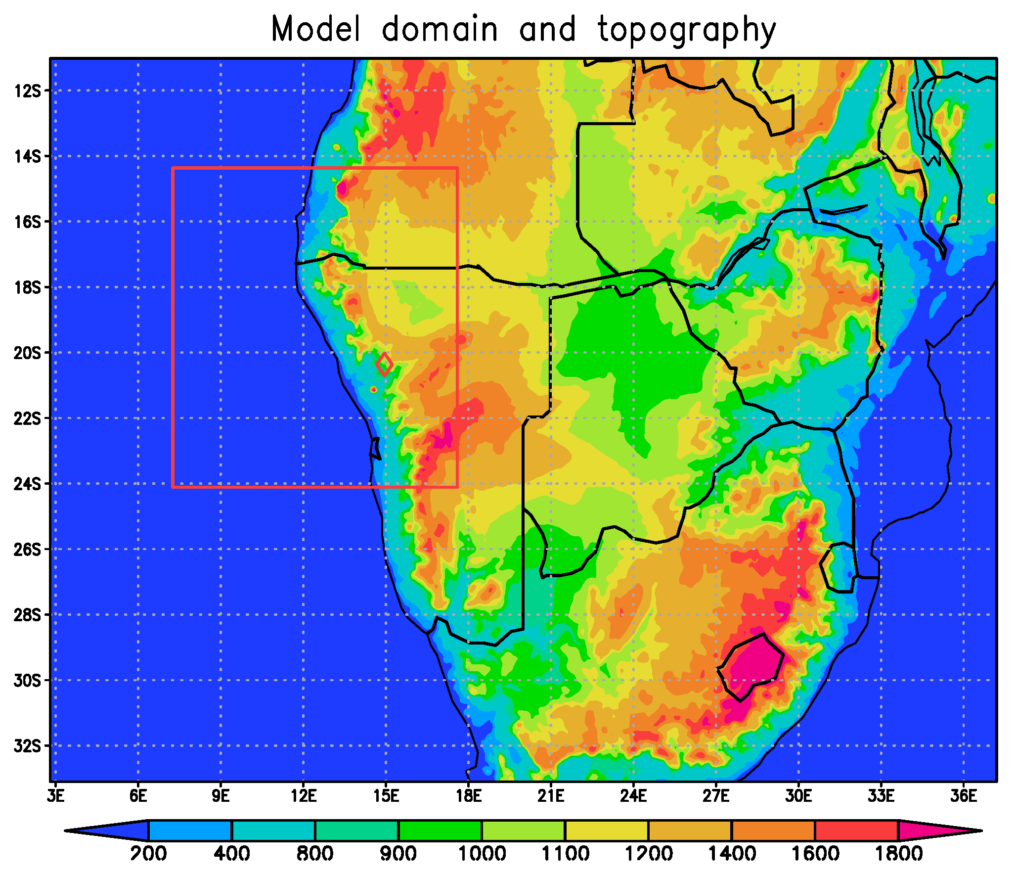
2. Model, Data and Simulations

The model used in this study is the Advanced Research Weather Research and Forecasting (WRF) (ARW) system, version 4.1.2 [31]. Given the location of Namibia in the lower latitudes, we have opted to use the tropical suite [32]. The tropical suite physics options include the Rapid Radiative Transfer Model (RRTM) for both shortwave and long wave radiation [33], Yonsei University (YSU) planetary boundary layer scheme [34], the new Tiedke cumulus scheme [35,36,37] and Weather Research and Forecasting Single Momentum 6-class microphysics scheme (WSM6) [38]. Ratna et al. [39] compared three different cumulus schemes over South Africa and found the Betts–Miller–Janjic scheme to outperform two other schemes. On the other hand, Crétat et al. [40] found Betts–Miller–Janjic to be the worst performing of the three cumulus schemes they tested over South Africa. It is not the intention of this study to determine the best schemes for Namibia, the physics options used in the study are the default tropical suite options. The new Tiedke cumulus scheme used in this study was not included in the comparison studies over Southern Africa, mentioned above. Sun and Bi [41] found the new Tiedke scheme to outperform other schemes in the simulation of the spatial rainfall distribution and diurnal cycle along the tropical belt. Gbode et al. [42] also found the new Tiedke scheme to be one of the best performer when simulating the surface air temperature and precipitation in the West African monsoon regime. The Global Forecast System (GFS) [43] which has a grid length of 0.25° is used to provide the initial conditions as well as lateral boundary conditions for WRF, every three hours of model simulation time. WRF is run from 23 October 2018 at 00 h 00 UTC until 25 October 2018 00 h 00 UTC, giving a simulation period of 48 h.
A summary of all the simulations made is shown in Table 1. A multi-grid nesting system is employed for three simulations, where a 9 km grid spacing domain is nested directly within GFS, and a child domain with a 3 km grid spacing is nested within the 9 km model. The 9 km parent domain spans 2°–37° E; and 33°–11° S, while the 3 km domain is located over 7°–17° E; 24°–14° S. Figure 1 shows the 9 km domain, while the red rectangle indicates a nest with a grid spacing of 3 km. The shaded colors indicate the topography of the domain, which shows that southern Africa has complex topography that should benefit from the use of high spatial resolution. The convection scheme was switched off for one of the 9 km grid-length simulations as well as its child domain (MNNOCU) resulting in a simulation that does not use a convection scheme at all. For the two 9 km simulations where the convection scheme was left on, the convection scheme was left on for one 3 km child domain (MNCU), and switched off for the other child domain (MN1CU). Two other simulations were conducted with a grid length of 3 km, nested directly within the GFS data, with a convection scheme on (SNCU) and off (SNNOCU). MN represents multi-nest, and SN represents single nest.
Hourly rainfall data from the Khorixas automatic rainfall station (ARS) of the NMS is used to show the timing and intensity of the rainfall event. Khorixas is located in the southern parts of the Kunene region. The 24 h simulated rainfall is compared to the Tropical Applications of Meteorology using SATellite data and ground-based observations (TAMSAT) rainfall estimates with a horizontal resolution of 4 km [44,45]. The 30 min interval Global Precipitation Measurement (GPM) rainfall calibrated with ground observations [46] with an approximate resolution of 0.1° is also used to study the timing of rainfall in satellite estimates. The latest climate reanalysis of European Centre for Medium Range Weather Forecasting (ECMWF) (ERA5) (0.25° grid length) [47] is also used in this study, where rainfall, temperature and wind speed and direction are also analyzed.

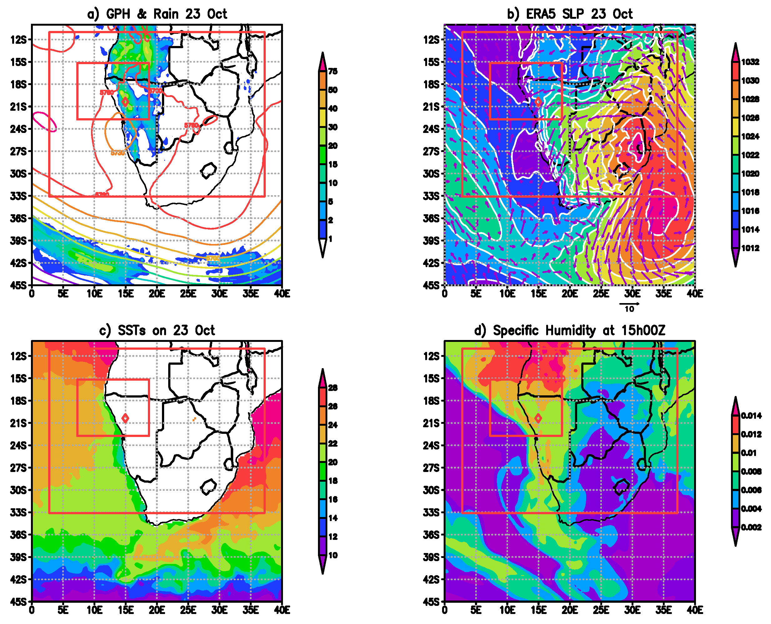
3. Event Description

The rainfall associated with the event was described by some as magical, because it fell after years of drought [48]. Figure 2a, shows the ERA5 500 hPa geopotential heights overlaying total rainfall on 23 October 2018. Rainfall fell over most of Namibia, with the largest amounts received in the northern parts of the country. The NMS hourly rainfall data for Khorixas indicated by a red diamond sign shows that 45.2 mm was received at 19 h 00 , followed by 5.7 mm at 20 h 00 and then 6.5 mm at 21 h 00 local time. This observation therefore indicates that the heavy rainfall event was short-lived, with most of the rainfall received within 1 h. The geopotential height shows that this rainfall occurred as a result of a cut-off low (COL) whose center can be seen on the border of Namibia and the Atlantic Ocean (Figure 2a). COLs are mid-latitude systems that can occur throughout the year, but they are observed to have a maximum in March to May and a second maximum later in the year [49,50]. These systems can affect Namibia, but, the northern parts of the country are not impacted as often as the southern parts of the country [15]. COLs can be associated with deep moist convection to the east of their trough axis as it appears was the case during this event.
Figure 2b shows the mean sea level pressure (MSLP), overlaid with the 10 m winds. The synoptic pattern shows a ridging Atlantic high-pressure system, has broken off the South Atlantic anticyclone to join the Indian Ocean high. There is a high-pressure system over the north-eastern part of South Africa which Ndarana et al. [51] have shown is a climatological feature whose flow and associated moisture fluxes are affected by ridging high-pressure systems. The ridging South Atlantic Ocean high as well as the high over the north-east of South Africa both act to transport moisture from the Indian Ocean over the land. The eastern parts of southern Africa are generally wetter because of the moisture from the Indian Ocean, which is also linked to the warmer sea surface temperatures (SSTs). Figure 2c shows a clear distinction between the Indian and Atlantic Ocean SSTs along the same lines of latitude with the Indian Ocean being warmer. The differences are due to the cold Benguela current in the Atlantic Ocean which transport cooler air from the poles to the region and the warm Agulhas current in the Indian Ocean which transports warmer air from the equator [12].
The winds appear to be easterly in general suggesting that some of the moisture responsible for the rainfall in Namibia, may have travelled all the way from the Indian Ocean to Namibia. However, according to Ndarana et al. [51] the rainfall associated with the ridging highs is mostly confined to the coastal regions. The wind pattern was plotted for different times of the day, and this pattern persists through most of the day. There are onshore arrows in the east of Khorixas which suggests some of the moisture may have originated from the Atlantic Ocean, which when combined with moisture associated with the ridging high cause convergence in the area where rainfall occurred. Figure 2d shows the specific humidity at 15h00 UTC, and indicates that the region between where ridging took place and Namibia where the rainfall event took place is mostly dry. The moisture is at a maximum over Angola and the adjacent Atlantic Ocean area which is associated with larger SST values. The area over Angola with higher values of specific humidity also experienced rainfall. This result suggests that some of the moisture that caused the rainfall could have been transported from north of Namibia.
All the simulations discussed in the study are nested within GFS three hourly data. The GFS simulated precipitable water and 500hPa geopotential heights are shown in the left panel of Figure 3, for (a) 06h00 UTC and (c) 15h00 UTC. The GFS captured the COL, and the area with the highest levels of precipitable water correspond with high values of specific humidity from ERA5 reanalysis. The second column of Figure 3 shows simulated MSLP overlaid with 10 m winds, for (b) 06h00 UTC and (d) 15h00 UTC. The strength of the high-pressure system over the eastern part of the country decreases between 06h00 and 15h00 UTC. In the Central-Western part of the country, the surface pressure decreased, indicating increased convergence in the afternoon. This circulation pattern supports the occurrence of rainfall in the afternoon. The results indicate that GFS was able to capture the synoptic systems, and compare well with the ERA5 reanalysis.

4. Results

This section is divided into three subsections. The first subsection, titled “Observations Comparison” compares the rainfall estimates from ERA5, GPM and TAMSAT for the event. The subsection is then followed by the “Effect of multi-nesting” and “Effect of the convection scheme”, respectively. The same figures will be referred to in the three subsections, back and forth.

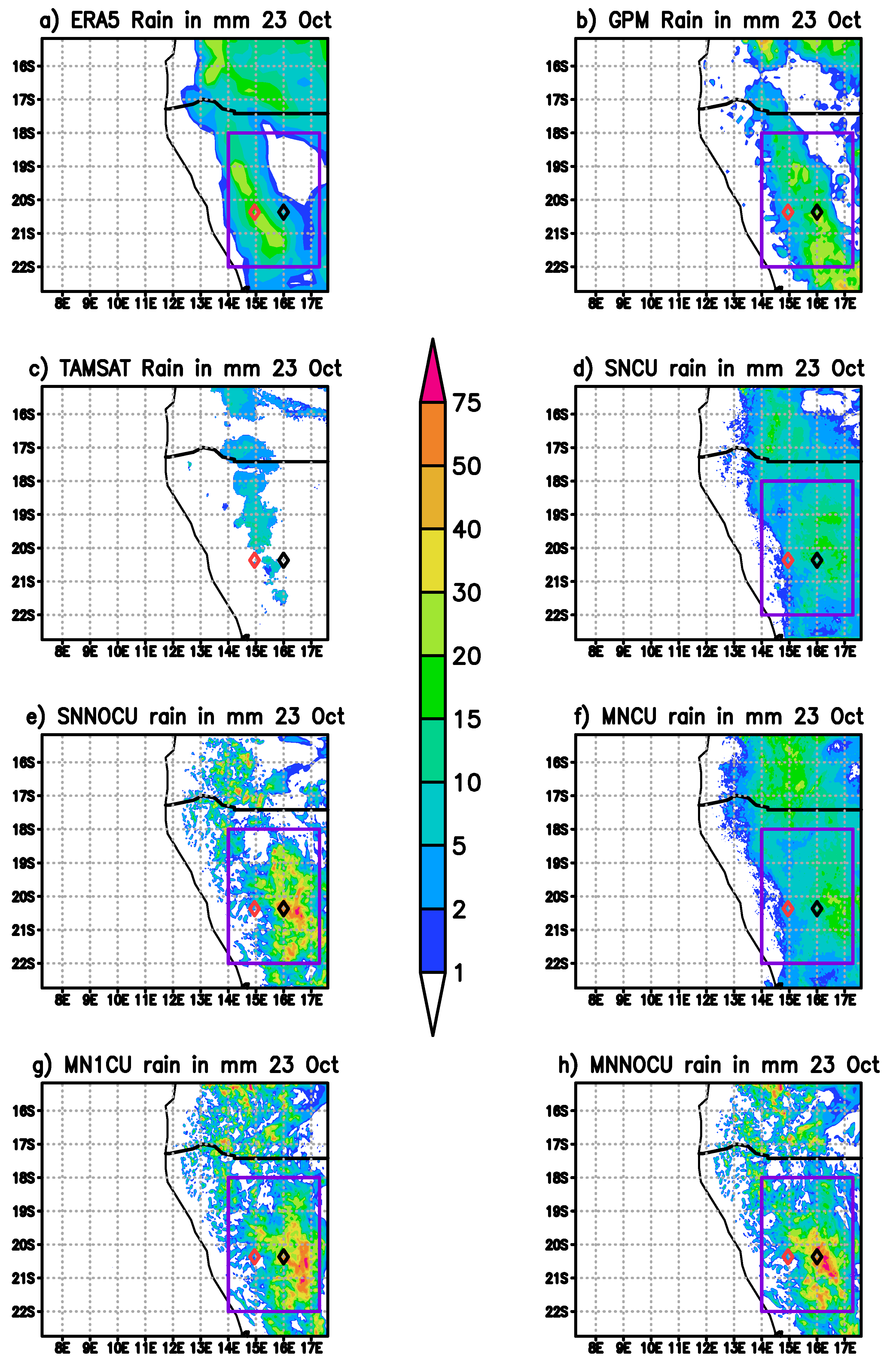
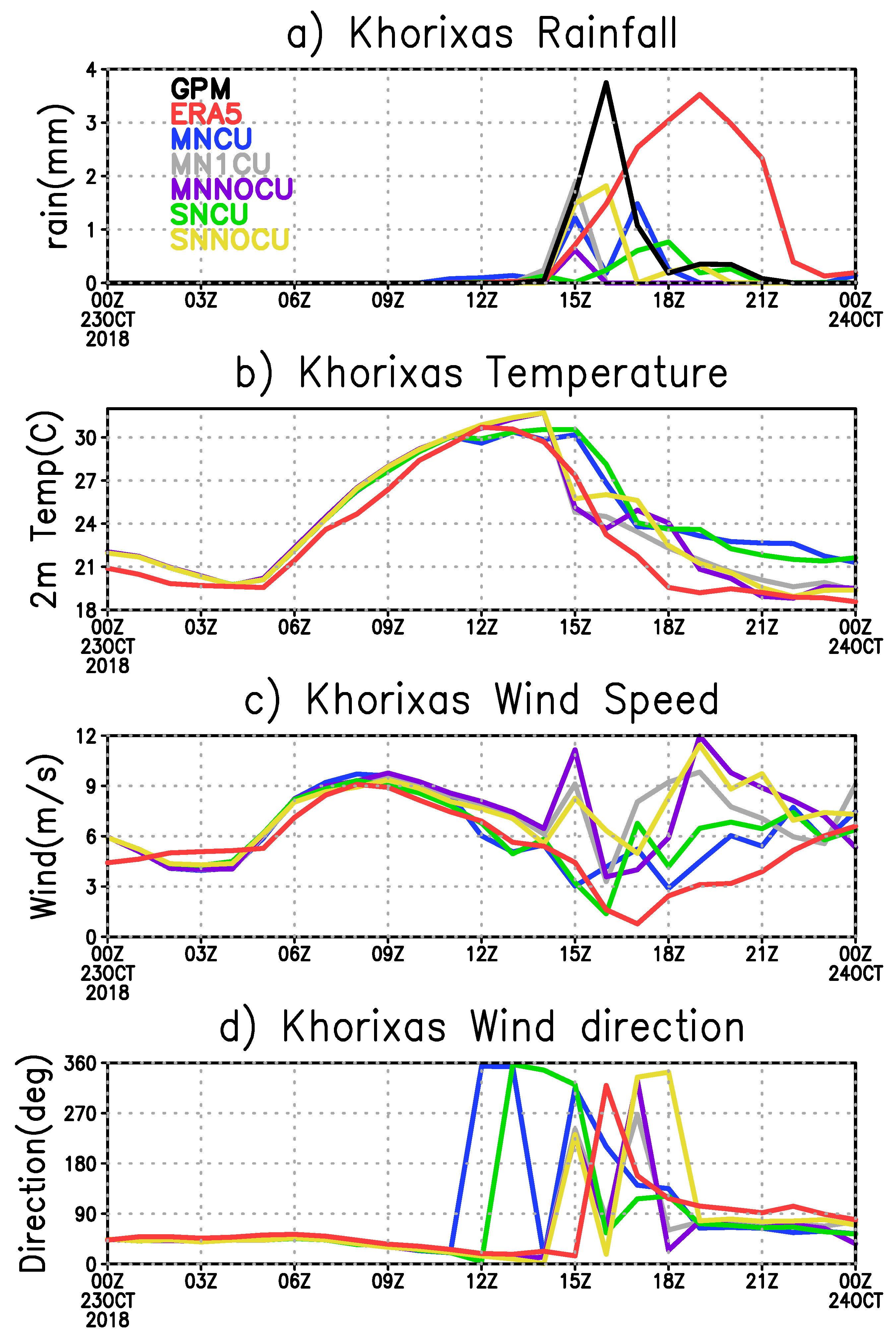
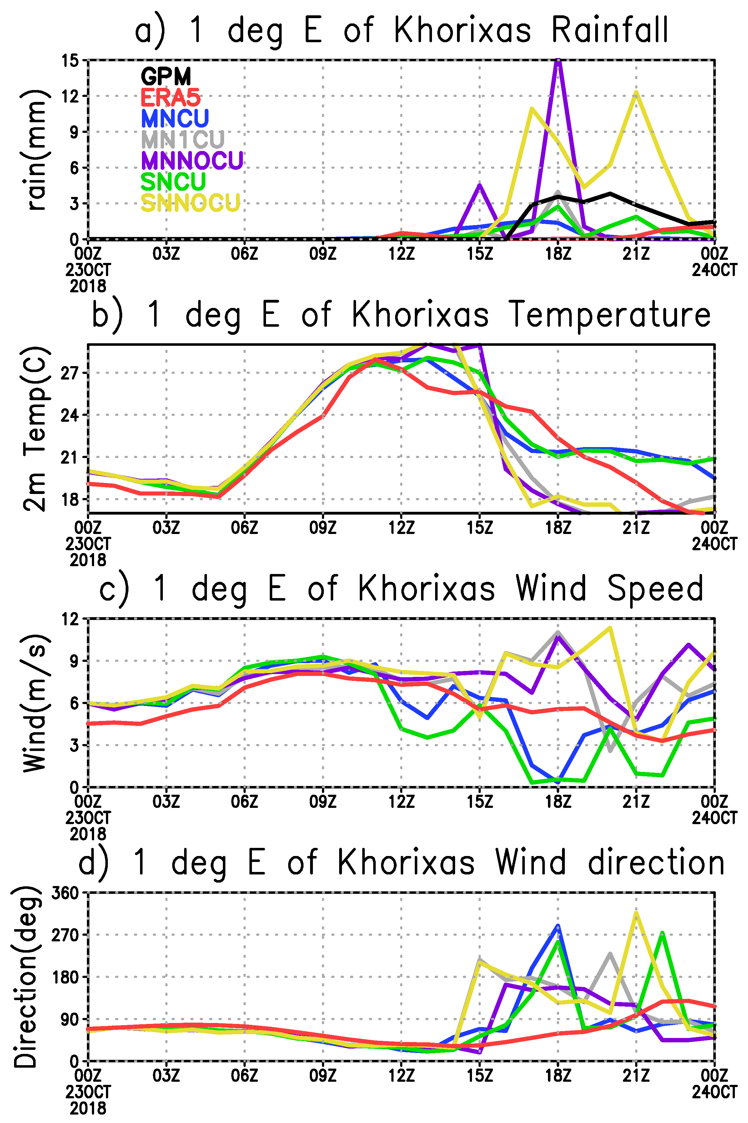
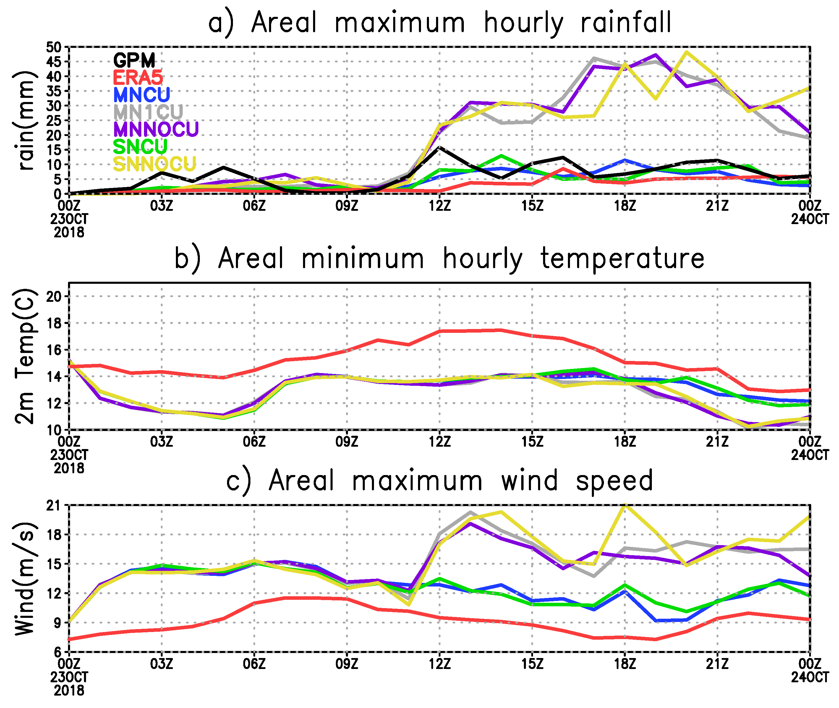
4.1. Observations Comparison

The 24-h rainfall total according to the ERA5 reanalysis, the GPM and TAMSAT satellite rainfall estimates are shown in Figure 4, as well as for different simulations. Khorixas which received over 50 mm of rainfall in less than three hours is shown by a red diamond sign in all the observations and simulation plots. The ERA5 reanalysis (Figure 4a) shows a north-west to south-east line of maximum rainfall of between 20 and 30 mm which is aligned with the position of Khorixas. The rainfall pattern extends from the domain border in the south, to the north beyond the border of Namibia and Angola. The GPM (Figure 4b) rainfall estimates also shows rainfall that extends between the two mentioned borders, with a pattern that is slightly different from that of the reanalysis. Khorixas is not observed to be associated with a large amount of rainfall according to GPM, with the largest amount of rainfall shown closer to the south-east border of the domain. The rainfall peak shown by GPM is larger than the ERA5 reanalysis. TAMSAT (Figure 4c) which provides the highest resolution of the three different observations captured substantially less rainfall than the other two observations. Khorixas is itself shown to not receive any rainfall according to this satellite rainfall estimate. However, the area shown to have received some rainfall (although little) is very close to Khorixas. Using Khorixas as our point of reference, ERA5 seems to have captured the location of the highest rainfall better than the two satellite estimates. Figure 1 has shown that there is some complex topography around Khorixas, and the result of this study agrees with the findings of Beck et al. [52] who indicates that the reanalysis outperforms GPM in regions of complex terrain.
A line plot using different variables was made for different observations and simulations to check the timing of heavy rainfall in the Khorixas vicinity (Figure 5). A maximum rainfall of 45.2 mm was reported at 17 h 00 UTC by the AWS at Khorixas (not shown). The GPM maximum is observed at 16 h 00 UTC, while the ERA5 maximum is predicted at 19 h 00 UTC, and therefore in terms of timing GPM seems to be slightly closer to the station observations (Figure 5a). The rainfall peak for both rainfall estimates is just below 4 mm, which is substantially lower than the point observation of 45.2 mm. The two are not directly comparable with the point observation because they represent an area average, with a grid length of about 10 km for GPM and about 27 km for ERA5. Due to the differences associated with the spatial data considered to be observations, we do not apply any verification nor skill scores in this study, but rather focus on understanding the processes associated with the event as simulated by different model configurations. This study also highlights a need for more ground observations, including radar that can provide three-dimensional cloud information to assist with model verification which can eventually assist with the improvement of model configurations so that they work as well as possible in the region.

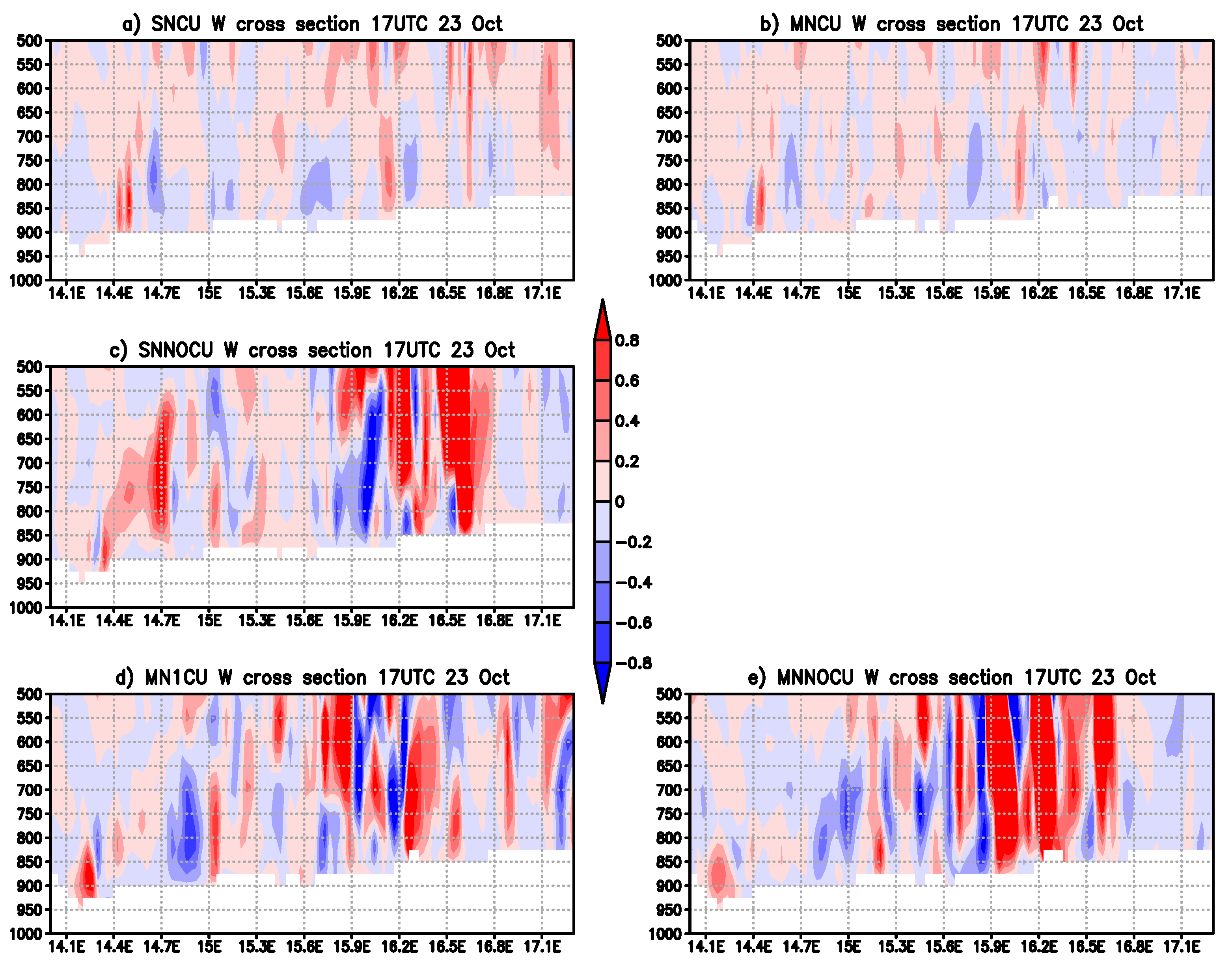
4.2. Effect of Multi-Nesting

In this study, we are able to produce simulations over Namibia with a grid spacing of 3 km, because of the limited area modelling procedure, which allows us to use less computational resources than would be needed for a global model running with the same grid length [22]. Laprise et al. [53] indicated that in the absence of strong surface forcing, the Limited Area Model (LAM) is incapable of correcting small-scale errors in the initial conditions and lack of information of small-scale processes in the LBCs. Time-dependent LBCs from a bigger domain or global model with lower resolution are applied to the lateral boundaries of the LAM. Warner et al. [54] recommended that the resolution of the large-scale and the nested model be as close as possible to reduce inconsistencies between the two models, to reduce gradients at the lateral boundaries which can generate gravity-inertia waves. Relaxation blends LBC’s and the LAM over several grid points for better matching of the two datasets, and the procedure also tends to damp noise [55,56]. The default setting of 4 columns and rows is used as the relaxation zone, in the lateral boundaries for this study. Larger differences in resolutions between the model providing the LBCs and the LAM are more prone to mismatches. Nesting the 3 km model directly within the GFS simulations implies that the ratio of the forcing data to the resolution used by the model is 9. Interpolation is made of GFS data with a grid spacing of about 27 km to the 3 km grid length, and interpolation errors maybe introduced. The WRF guidance is that one should use a ratio of between 3 and 5, for best results, which is why a multi-nesting procedure is usually applied to avoid reflection of atmospheric waves at the domain boundaries. With the multi-nesting procedure interpolation is made from GFS 27 km to 9 km, and then to 3 km which can potentially limit interpolation errors.
In Figure 1 we showed that the terrain of southern Africa is complex, and the use of high-resolution assists with a better representation of the topography. The 9 km domain was made very large especially on the eastern side to include a larger land area so that the topography is allowed to impact the simulation result. The winds were shown to be mostly north-easterly to easterly, but indications are that moisture was also transported from the west in the Atlantic Ocean and from Angola in the north. The higher resolution topography will therefore have influenced the flow coming from the east and the north, while the flow from the ocean would mostly not be impacted. Figure 4d represents a single nest with a grid length of 3 km, and the convection scheme switched on (SNCU), while Figure 4f shows a multi-nest with a convection scheme on for both the 9 km resolution parent domain and 3 km child domain simulation (MNCU).
There are large similarities in the two simulations regarding the location of the rainfall. There are small differences in the extreme north-eastern part of the domain where the SNCU captured less rainfall. The rainfall produced by MNCU is slightly more than the SNCU simulated amount east of the two diamonds as well as towards the northern border of the domain in Angola. The red diamond represents Khorixas, the station for which we have hourly rainfall data. All the plots indicate that more rainfall is simulated east of Khorixas. Figure 1 shows that the areas associated with higher rainfall are associated steeper topography than Khorixas. Figure 5 plots indicate that less rainfall was simulated over Khorixas, than about 1° E of Khorixas (Figure 6), which is selected as an example point. The same analysis was made for three other points, north-east, south-east and 2° E of Khorixas and the results agree with those shown for Figure 6. Line plots were made for Khorixas and for one example grid point where a greater amount of rainfall seems to be simulated. The dark blue line represents MNCU while the green line represents SNCU (Figure 5a). MNCU which appeared to have slightly more rainfall is associated with two small peaks with the timing of the second rainfall peak matching the timing of the observed rainfall peak. The SNCU rainfall peak occurs an hour later than the observations with a smaller peak compared to the MNCU simulations. Both simulations produced some rainfall 1° east of Khorixas again with MNCU rainfall being simulated earlier than SNCU. Line graphs were also made for temperature (Figure 5b), wind speed (Figure 5c) and wind direction (Figure 5d). The temperature dropped when rainfall is simulated, and with the two simulations, the wind speed decreased just before the rainfall event and picked up later. The wind direction changed from north-easterly to north-westerly, with changes occurring earlier with the MNCU simulation. The blue and green lines are generally close to one another for all the variables indicating that the impact of multi-nesting versus a single nest is smaller for the case being studied here, compared to impact of the convection scheme.
Figure 4e represents the single nest simulation with the convection scheme off (SNNOCU) while Figure 4g represents the multi-nest with the convection scheme left on for the 9 km grid-length simulation and switched off for the 3 km grid length (MN1CU). MN1CU represents what would be considered to be an ideal simulation because the parent-child domain nesting ratio is 3, and the convection scheme is switched off for the 3 km grid spacing simulations which follows the modelling guidelines provided by model developers. Both configurations produced more rainfall east of Khorixas in a pattern that differs from both GPM and ERA5. The SNNOCU configuration produced a lot less rainfall in the north of the domain, and in some cases, the rainfall is seen in both the ERA5 and GPM estimates. For the selected grid points, SNNOCU generally produces more rainfall than MN1CU. Over Khorixas, the timing of the rainfall peak was simulated two hours early by MN1CU and one hour early by the SNNOCU simulation (Figure 5a). Regarding the temperature, wind speed and wind direction lines, the two configurations are generally similar. Champion and Hodges [23] nested a 12 km, 4 km and 1.5 km grid spacing simulations using multi-nesting technique as well as directly inside the lower resolution global model with a grid length of 25 km. Nesting differently resulted in the rainfall location being different among simulations.
We have also plotted hourly maximum rainfall between 14° and 17.3° E, and from 22° to 18° S (area shown by purple rectangle in Figure 3) for different observations and simulations. Figure 7a shows that the simulated maximum rainfall for the green (SNCU) and blue (MNCU) lines is mostly, similar. The yellow line which represents SNNOCU is mostly aligned with the MN1CU, and MNNOCU lines further confirming that multi-nesting results in a smaller difference in the simulations. The same applies for the minimum hourly temperature where SNCU and MNCU are mostly aligned and warmer than other simulations after the highest area maximum rainfall is received (Figure 7b). The 10 m maximum wind speed is smaller in the SNCU and MNCU compared to other configurations (Figure 7c).

4.3. Effect of the Convection Scheme

Lower resolution models rely on convection schemes [20] to represent the effects of convection on large-scale processes and to prevent unstable growth of cloudy structures on the grid [28]. Convective scale models on the other hand are expected to capture cloud structures explicitly. There is however no clear-cut distinction between models that should use a convection scheme and those that should not, and different procedures have variously been applied. Some studies have indicated that a grid spacing of about 4 km should be sufficient to resolve much of the mesoscale structure and evolution of some convective systems (e.g., [57,58]). Roberts [59] found a grid spacing of 1 km to produce much better simulations than 4 km and recommended the use of a grid spacing of 1 km to represent the dynamics of localized thunderstorms and local processes responsible for triggering the event. Bryan et al. [60] argues that a grid spacing of order 100 m is required to simulate the squall-line structures and their evolution with skill. Some studies use a form of convection scheme (e.g., [29]) when using a grid spacing of 4 km or similar, and these have been found to give better results than when the convection parametrization is switched off [28]. No-convection scheme was used in some studies when a grid spacing of 1.5 km is employed (e.g., [23,61]). The WRF guidance notes recommend switching off convection schemes for a grid spacing of 3 km and less.
Simulations with a single nest and multi-nest were conducted with and without a convection scheme at a grid spacing of 3 km. The convection scheme used in this study is the new Tiedke scheme (option 16 in the WRF namelist) [35,36,37]. The new Tiedke scheme includes cloud water, cloud ice and momentum tendencies and has shallow convection. A total of five simulations are compared, with SNCU and SNNOCU looked at together to study the impact of switching the convection scheme off with a grid spacing of 3 km in a single nest. MNNOCU, MN1CU and MNCU are all compared to analyze the impact of switching off the cumulus scheme when a grid spacing of 9 km and 3 km are used. When running a model with a convection scheme on, there are two components to the precipitation, namely the convective precipitation generated by the convection scheme and large-scale precipitation captured explicitly by the model [23]. Figure 8b shows the total precipitation from the 9 km and 3 km child domains when the convection scheme is switched on. High intensity rainfall is only simulated in the north parts of the domain in Angola. When the convection scheme is switched on the model does not simulate much high intensity rainfall in Namibia.
Figure 8c shows convection scheme produced rainfall outside the red box, and grid scale rainfall inside the red box. Unlike with Figure 8b where there is no clear benefit of using a grid spacing 3 km in the red box compared to the larger domain, there is a difference between the simulation in the red box and the outer domain in Figure 8c. Higher rainfall intensities are simulated east of Khorixas in this simulation. For Figure 8d the convection scheme was switched off for the 9 km grid as well, and this has resulted in high rainfall intensities outside the red box in Angola. High intensities are also found east of Khorixas, over higher lying areas compared to Khorixas. Champion and Hodges [23] also found that switching off the parametrization scheme resulted in increased area averaged precipitation intensities as well as increased details. The GPM rainfall estimate (Figure 8a) shows high rainfall intensity areas in Angola; however these extend further east than in the simulations.
Figure 4 shows different observations as well as different simulation in the red box that was discussed in Figure 8. A comparison between Figure 4d,e shows that switching off the convection scheme results in more details and higher rainfall values. The same result is found for the multi-nest simulation, where greater detail is visible in Figure 4g. Forcing the 3 km model with a 9 km model with the convection scheme on (Figure 4g) and off (Figure 4h) does not result in very large differences between the two simulations. The location of high rainfall intensities is different among different simulations, with a general agreement of the location being to the east of Khorixas. In general, convective scale models are not expected to capture the exact location of the storms, which is why rainfall verification of convective scale storms uses object-based verification as opposed to traditional grid point verification statistics to avoid penalizing the model twice (e.g., [62]).
Figure 5 and Figure 6 respectively show line graphs of hourly rainfall, temperature, wind speed and direction for Khorixas and 1° to the east of Khorixas where larger rainfall intensities were simulated by most configurations. The blue and green lines indicate configurations where the convection scheme was switched on with a 3 km grid spacing. The two lines are generally similar and associated with the least amount of rainfall as was shown on the spatial plots where smaller intensities were simulated over most of the domain. The drop in temperature due to the rainfall event is smaller compared to the configurations where the convection scheme is switched off. Both configurations result in lower wind speeds, associated with the event. The wind direction changed from north-eastern to north-westerly in both configurations hours before the rainfall was captured. There is no indication that the presence of the convection scheme resulted in an earlier triggering of the rainfall event because the timing of peak rainfall is generally similar to configurations where the convection scheme is turned off.
The maximum areal rainfall plot (Figure 7a) shows that all the 3 km simulations with the convection scheme off resulted in rainfall of about 40 to 45 mm. When the convection scheme is on, the simulated maximum rainfall does not exceed 15 mm. The configurations with no-convection scheme, result in lower temperatures (Figure 7b) and stronger maximum wind speed (Figure 7c). Previous idealized studies (e.g., [63]) have shown that more rainfall is associated with stronger downdrafts, and a cooler and stronger cold pool. Figure 9 shows the vertical wind cross section at 17 h 00 UTC at line of latitude, 20.366° S, which is same line where Khorixas is located. The east-west extend is similar to the purple box shown in Figure 4. The white area at the bottom of Figure 9 panels shows that the altitude of the land surface relative to sea level, occurs at a higher altitude as one moves towards the east. The top two plots Figure 9a,b where the convection scheme is switched on are associated with smaller updrafts and downdrafts. The color range was kept low to allow some detail in these two plots where the convection scheme is switched off. The updrafts and downdrafts are much stronger in the three simulations shown in Figure 9c–e, where the convection scheme is switched off. The simulations with the convection scheme on, resulted in less rainfall, less cooling and their associated cold pool is warmer and the wind speed lower than configurations with the convection scheme off. These results raise questions about the applicability of the new Tiedke scheme at these resolutions. The change in direction shown in Figure 5 and Figure 6 after it started raining were associated with the cold pool.

5. Summary and Conclusions

In this study, we investigate a heavy rainfall event over the north-western parts of Namibia in the Kunene region as simulated by the WRF model. The event was associated with a cut-off low with moisture converging over the region from the northeast and east of the sub-region and southwest from the Atlantic Ocean. The rainfall event was very short-lived with more than 45 mm received over Khorixas within one hour, and no rainfall observed whatsoever three hours later. To our knowledge no other NWP study has been published with a focus on the Kunene region or on Namibia in general. Simulations were forced with the GFS data with a grid spacing of 0.25°, using multi-nesting with a 9 km-mesh parent domain and a child domain using 3 km horizontal grid spacing. The GFS captured the synoptic circulation and moisture distribution well, which shows the WRF was forced with realistic large-scale conditions. The location of the high rainfall intensities in the single and multi-nest simulations were slightly different, but there are general similarities between the two simulations. Champion and Hodges [23] tested the impact of nesting the Unified Model (UM) LAM simulations inside multi-nest using grid spacing of 1.5 km, 4 km and 12 km and nesting directly from the global data, and also found the rainfall location to differ among different simulations. They recommended the use of a series of nested resolutions as part of an optimal configuration to reduce uncertainty in the precipitation over time. We recommend that more tests be conducted to test the value of multi-nesting. In a sister study conducted over Botswana, the use of a multi-nest seemed to generate a mesovortex in the coarse-grid domain that was not found in the observations [64].
The study also investigated the impact of switching on the convection scheme when using a grid spacing of 3 km. The use of a convection scheme at this scale is contested among scientists with some indicating that 4 km is sufficient to capture bulk dynamics of squall-lines [58], others suggesting the use of a grid length of approximately 1 km [59] and still others proposing the use of order 100 m [60]. The WRF notes recommend switching off the convection scheme when using a grid spacing of 3 km or less, although they note that early triggering that is usually associated with the convection schemes may be necessary. The largest differences in the study are between simulations using the no-convection configuration versus those with the convection scheme. Leaving the convection scheme on with a grid spacing of 3 km does not seem to provide the extra benefit of using high resolution, providing little detail in the simulations. Switching off the convection scheme even with a grid spacing of 9 km provides more detail than keeping the convection scheme on with a 3 km grid spacing. The no-convection scheme simulations are also associated with larger rainfall intensities as was also found by Champion and Hodges [23]. The convection scheme used in this study is the new Tiedke scheme [35,36,37] which is selected as part of the tropical physics suite. Recently, Steeneveld and Peerlings [21] found a scale-aware convection scheme to perform better than others in simulating a severe thunderstorm event in the Netherlands using a grid spacing of 2 km and 4 km. This result points to a limitation in our study that is specific to the new Tiedke scheme and a case with a strong synoptic forcing. We recommend further tests with different convection schemes and for different heavy rainfall cases triggered by different weather systems that bring rainfall over Namibia. This type of study is useful to assist the NMS to understand the pros and cons associated with using different configurations to produce severe weather forecasts.
In future work, given a lack of observational data to better evaluate high-resolution simulations, use of all-sky satellite radiance observations with satellite simulators would be a promising approach to further evaluate forecasting skill, especially where ground-based radar networks are insufficient [65]. In addition, high-resolution ensemble forecasting and ensemble-based data assimilation methods are promising approaches to improve forecasting skill for intense precipitation events [28,66]. The incremental value added by feasible implementation of such approaches by the NMS would also require observational evaluation.

Author Contributions

M.-J.M.B., S.S., A.F. and T.M. conceptualized the study, S.S., A.L., S.M., R.M. implemented WRF model (software), M.-J.M.B., T.N., E.P. and S.S. made formal analysis, A.L., S.M. and E.R. provided computational resources, M.M.B and E.R. acquired funding, M.-J.M.B. wrote original draft, S.S., T.N., A.F., T.M., R.M. reviewed and edited the text. All authors have read and agreed to the published version of the manuscript.

Funding

This research was partially funded through the Climate Research for Development (CR4D) fellowship grant number CR4D-19-11 managed by the African Academy of Sciences. The work is also supported by the South African Department of Science and Innovation.

Acknowledgments

The authors acknowledge the University of Namibia and the South African Centre for High Performance Computing (CHPC) for use of their HPC systems, and Namibia Meteorological Services for availing station observations.

Conflicts of Interest

The authors declare no conflict of interest. The funders had no role in the design of the study; in the collection, analyses, or interpretation of data; in the writing of the manuscript, or in the decision to publish the results.

References

  1. Reid, H.; Sahlén, L.; Stage, J.; Macgregor, J. Climate change impacts on Namibia’s natural resources and economy. Clim. Policy 2008, 8, 452–466. [Google Scholar] [CrossRef]
  2. Mulwa, C.; Visser, M. Farm diversification as an adaptation strategy to climatic shocks and implications for food security in northern Namibia. World Dev. 2020, 129, 104906. [Google Scholar] [CrossRef]
  3. Teweldemedhin, M.; Durand, W.; Crespo, O.; Beletse, Y.; Nhemachena, C. Economic impact of climate change and benefit of adaptations for maize production: Case from Namibia, Zambezi region. J. Dev. Agric. Econ. 2015, 7, 61–71. [Google Scholar] [CrossRef] [Green Version]
  4. Newsham, A.; Thomas, D. Knowing, farming and climate change adaptation in North-Central Namibia. Glob. Environ. Chang. 2011, 21, 761–770. [Google Scholar] [CrossRef] [Green Version]
  5. Tyson, P. Climatic Change and Variability in Southern Africa; Oxford University Press: Oxford, UK, 1986; p. 220. [Google Scholar]
  6. Mason, S.; Jury, M. Climatic variability and change over southern Africa: A reflection on underlying processes. Prog. Phys. Geog. 1997, 21, 23–50. [Google Scholar] [CrossRef]
  7. Howard, E.; Washington, R. Characterizing the synoptic expression of the angola low. J. Clim. 2018, 31, 7147–7165. [Google Scholar] [CrossRef]
  8. Vigaud, N.; Pohl, B.; Crétat, J. Tropical-temperate interactions over Southern Africa simulated by a regional climate model. Clim. Dyn. 2012, 39, 2895–2916. [Google Scholar] [CrossRef]
  9. Walker, N. Links Between South African Summer Rainfall and Temperature Variability of the Agulhas and Benguela Current Systems. J. Geophys. Res. 1990, 95, 3297–3319. [Google Scholar] [CrossRef]
  10. Harrison, M. A generalised classification of South African Summer rain bearing synoptic systems. J. Climatol. 1984, 4, 547–560. [Google Scholar] [CrossRef]
  11. Todd, M.; Washington, R. Circulation anomalies with tropical-temperate troughs in Southern Africa and the South West Indian Ocean. Clim. Dyn. 1999, 15, 937–951. [Google Scholar] [CrossRef]
  12. Tyson, P.; Preston-Whyte, R.A. The Weather and Climate of Southern Africa; Oxford University Press: Oxford, UK, 2000; p. 396. [Google Scholar]
  13. Engelbrecht, F.A.; Adegoke, A.; Bopape, M.; Naidoo, M.; Garland, R.; Thatcher, M.; Katzfey, J.; Werner, M. Projections of rapidly rising surface temperatures over Africa under low mitigation. Environ. Res. Lett. 2015, 10, 085004. [Google Scholar] [CrossRef]
  14. IPCC. Technical Summary: Global Warming of 1.5 °C. An IPCC Special Report on the Impacts of Global Warming of 1.5 C above Pre-Industrial Levels and Related Global Greenhouse Gas Emission Pathways, in the Context of Strengthening the Global Response to the Threat of Climate Change, Sustainable Development, and Efforts to Eradicate Poverty; IPCC: Paris, France, 2018. [Google Scholar]
  15. Dirkx, E.; Hager, C.; Tadross, M.; Bethune, S.; Curtis, B. Climate Change Vulnerability & Adaptation Assessment Namibia; Desert Research Foundation Namibia & Climate Systems Analysis Group, UCT: Cape Town, South Africa, 2008. [Google Scholar]
  16. Ellis, H.; Matjila, J. After Devastating Floods, Namibians Fight Cholera and Wait for a Return to Normalcy. UNICEF info by Country; UNICEF: Geneva, Switzerland, 2008. [Google Scholar]
  17. Government of the Republic of Namibia. Post Disaster Needs Assessment (PDNA); Government of the Republic of Namibia: Windhoek, Namibia, 2009.
  18. Bauer, P.; Thorpe, A.; Brunet, G. The quiet revolution of numerical weather prediction. Nature 2015, 525, 47–55. [Google Scholar] [CrossRef] [PubMed]
  19. Holton, J.R.; Hakim, G. An Introduction to Dynamic Meteorology; Academic Press: Cambridge, MA, USA, 2014; p. 552. [Google Scholar]
  20. Stensrud, D. Parametrization schemes. Keys to understanding numerical weather prediction models. Reprint of the 2007 hardback ed.; In Parameterization Schemes: Keys to Understanding Numerical Weather Prediction Models; Elsevier: Amsterdam, The Netherlands, 2007; p. 480. [Google Scholar] [CrossRef]
  21. Steeneveld, G.J.; Peerlings, E. Mesoscale Model Simulation of a Severe Summer Thunderstorm in The Netherlands: Performance and Uncertainty Assessment for Parameterised and Resolved Convection. Atmosphere 2020, 11, 811. [Google Scholar] [CrossRef]
  22. Staniforth, A. Regional modeling: A theoretical discussion. Meteorol. Atmos. Phys. 1997, 63, 15–29. [Google Scholar] [CrossRef]
  23. Champion, A.; Hodges, K. Importance of resolution and model configuration when downscaling extreme precipitation. Tellus A 2014, 66. [Google Scholar] [CrossRef] [Green Version]
  24. Wang, Y.; Leung, L.; McGregor, J.; Lee, D.K.; Wang, W.C.; Ding, Y.; Kimura, F. Regional Climate Modeling: Progress, Challenges, and Prospects. J. Meteorol. Soc. Jpn. 2004, 82, 1599–1628. [Google Scholar] [CrossRef] [Green Version]
  25. Bopape, M.M.; Sithole, H.; Motshegwa, T.; Rakate, E.; Engelbrecht, F.; Morgan, A.; Ndimeni, L.; Botai, O.J. A Regional Project in Support of the SADC Cyber-Infrastructure Framework Implementation: Weather and Climate. Data Sci. J. 2019, 18, 34. [Google Scholar] [CrossRef] [Green Version]
  26. Motshegwa, T.; Wright, C.; Sithole, H.; Ngolwe, C.; Morgan, A. Developing a Cyber-infrastructure for Enhancing Regional Collaboration on Education, Research, Science, Technology and Innovation. In Proceedings of the 2018 IST-Africa Week Conference (IST-Africa), Gaborone, Botswana, 9–11 May 2018; pp. 1–9. [Google Scholar]
  27. Wu, X.; Li, X. A review of cloud-resolving model studies of convective processes. Adv. Atmos. Sci. 2008, 25, 202–212. [Google Scholar] [CrossRef]
  28. Clark, P.; Roberts, N.; Lean, H.; Ballard, S.; Charlton-Perez, C. Convection-permitting models: A step-change in rainfall forecasting. Meteorol. Appl. 2016, 23. [Google Scholar] [CrossRef] [Green Version]
  29. Woodhams, B.; Birch, C.; Marsham, J.; Bain, C.; Roberts, N.; Boyd, D. What is the added-value of a convection-permitting model for forecasting extreme rainfall over tropical East Africa? Mon. Weather Rev. 2018, 146. [Google Scholar] [CrossRef]
  30. Xu, K.M.; Cederwall, R.; Donner, L.; Grabowski, W.W.; Guichard, F.; Johnson, D.; Khairoutdinov, M.; Krueger, S.; Petch, J.; Randall, D.; et al. An Intercomparison of Cloud-Resolving Models with the ARM Summer 1997 IOP Data. Q. J. R. Meteorol. Soc. 2001, 128, 593–624. [Google Scholar] [CrossRef] [Green Version]
  31. Skamarock, W.C.; Klemp, J.B.; Dudhia, J.; Gill, D.O.; Liu, Z.; Berner, J.; Huang, X.Y. A Description of the Advanced Research WRF Model Version 4 (No. NCAR/TN-556+STR); National Center for Atmospheric Research: Boulder, CO, USA, 2019. [Google Scholar]
  32. Wang, W. WRF: More Runtime Options; WRF Tutorial; UNSW: Sydney, Australia, 2017; p. 46. [Google Scholar]
  33. Iacono, M.; Delamere, J.; Mlawer, E.; Shepard, M.; Clough, S.; Collins, W. Radiative Forcing by Long-Lived Greenhouse Gases: Calculations with the AER Radiative Transfer Models. J. Geophys. Res. 2008, 113. [Google Scholar] [CrossRef]
  34. Hong, S.Y.; Noh, Y.; Dudhia, J. A New Vertical Diffusion Package with an Explicit Treatment of Entrainment Processes. Mon. Weather Rev. 2006, 134, 2318–2341. [Google Scholar] [CrossRef] [Green Version]
  35. Tiedtke, M. A Comprehensive Mass Flux Scheme For Cumulus Parameterization In Large-Scale Models. Mon. Weather Rev. 1989, 117. [Google Scholar] [CrossRef] [Green Version]
  36. Zhang, C.; Wang, Y.; Hamilton, K. Improved Representation of Boundary Layer Clouds over the Southeast Pacific in ARW-WRF Using a Modified Tiedtke Cumulus Parameterization Scheme*. Mon. Weather Rev. 2011, 139, 3489–3513. [Google Scholar] [CrossRef] [Green Version]
  37. Zhang, C.; Wang, Y. Projected Future Changes of Tropical Cyclone Activity over the Western North and South Pacific in a 20-km-Mesh Regional Climate Model. J. Clim. 2017, 30, 5923–5941. [Google Scholar] [CrossRef]
  38. Hong, S.Y.; Kim, J.H.; Lim, J.O.; Dudhia, J. The WRF single moment microphysics scheme (WSM). J. Korean Meteorol. Soc. 2006, 42, 129–151. [Google Scholar]
  39. Ratna, S.; Ratnam, J.V.; Behera, S.; Rautenbach, C.; Ndarana, T.; Takahashi, K.; Yamagata, T. Performance assessment of three convective parameterization schemes in WRF for downscaling summer rainfall over South Africa. Clim. Dyn. 2013, 42, 358. [Google Scholar] [CrossRef] [Green Version]
  40. Crétat, J.; Pohl, B.; Richard, Y.; Drobinski, P. Uncertainties in simulating regional climate of Southern Africa: Sensitivity to physical parameterizations using WRF. Clim. Dyn. 2011, 38, 613–634. [Google Scholar] [CrossRef]
  41. Sun, B.Y.; Bi, X. Validation for a tropical belt version of WRF: Sensitivity tests on radiation and cumulus convection parameterizations. Atmos. Ocean. Sci. Lett. 2019, 1–9. [Google Scholar] [CrossRef] [Green Version]
  42. Gbode, I.; Dudhia, J.; Vincent, A. Sensitivity of different physics schemes in the WRF model during a West African monsoon regime. Theor. Appl. Climatol. 2018, 1–19. [Google Scholar] [CrossRef] [Green Version]
  43. Sela, J. Implementation of the sigma pressure hybrid coordinate into GFS. Ncep Off. Note 2009, 461, 1–25. [Google Scholar]
  44. Maidment, R.; Grimes, D.; Black, E.; Tarnavsky, E.; Young, M.; Greatrex, H.; Allan, R.; Stein, T.; Nkonde, E.; Senkunda, S.; et al. A new, long-term daily satellite-based rainfall dataset for operational monitoring in Africa. Sci. Data 2017, 4. [Google Scholar] [CrossRef]
  45. Tarnavsky, E.; Grimes, D.; Maidment, R.; Black, E.; Allan, R.; Stringer, M.; Chadwick, R.; Kayitakire, F. Extension of the TAMSAT Satellite-Based Rainfall Monitoring over Africa and from 1983 to Present. J. Appl. Meteorol. Clim. 2014, 53, 2805–2822. [Google Scholar] [CrossRef] [Green Version]
  46. Huffman, G.; Bolvin, D.; Braithwaite, D.; Hsu, K.; Joyce, R.; Xie, P. Integrated Multi-SatellitE Retrievals for GPM (IMERG), Version 4.4.; NASA’s Precipitation Processing Center, NASA: Greenbelt, MD, USA, 2014.
  47. Hersbach, H.; Dee, D. ERA5 Reanalysis is in Production; ECMWF: Reading, UK, 2016. [Google Scholar]
  48. Chawane, G. Watch: Magnificent Namibia river flood after years of drought. The Citizen, 24 October 2018. [Google Scholar]
  49. Singleton, A.; Reason, C. Variability in the characteristics of cut-off low pressure systems over subtropical southern Africa. Int. J. Climatol. 2007, 27, 295–310. [Google Scholar] [CrossRef]
  50. Ndarana, T.; Rammopo, T.S.; Chikoore, H.; Barnes, M.A.; Bopape, M.J. A quasi-geostrophic diagnosis of the zonal flow associated with cut-off lows over South Africa and surrounding oceans. Clim. Dyn. 2020, 55, 2631–2644. [Google Scholar] [CrossRef]
  51. Ndarana, T.; Mpati, S.; Bopape, M.J.; Engelbrecht, F.; Chikoore, H. The flow and moisture fluxes associated with ridging South Atlantic Ocean anticyclones during the subtropical southern African summer. Int. J. Climatol. 2020. [Google Scholar] [CrossRef]
  52. Beck, H.; Pan, M.; Roy, T.; Weedon, G.; Pappenberger, F.; van Dijk, A.; Huffman, G.; Adler, R.; Wood, E. Daily evaluation of 26 precipitation datasets using Stage-IV gauge-radar data for the CONUS. Hydrol. Earth Syst. Sci. 2019, 23, 207–224. [Google Scholar] [CrossRef] [Green Version]
  53. Laprise, R.; RaviVarma, M.; Denis, B.; Caya, D.; Zawadzki, I. Predictability of a Nested Limited-Area Model. Mon. Weather Rev. 2000, 128, 4149–4154. [Google Scholar] [CrossRef]
  54. Warner, T.T.; Peterson, R.A.; Treadon, R.E. A Tutorial on Lateral Boundary Conditions as a Basic and Potentially Serious Limitation to Regional Numerical Weather Prediction. Bull. Am. Meteorol. Soc. 1997, 78, 2599–2618. [Google Scholar] [CrossRef] [Green Version]
  55. Davies, H.; Turner, R. Sensitivity Updating prediction models by dynamical relaxation: An examination of the technique. Q. J. R. Meteorol. Soc. 1977, 103, 225–245. [Google Scholar] [CrossRef]
  56. Davies, T. Lateral boundary conditions for limited area models. Q. J. R. Meteorol. Soc. 2014, 140. [Google Scholar] [CrossRef]
  57. Khairoutdinov, M.F.; Randall, D.A. A cloud resolving model as a cloud parameterization in the NCAR Community Climate System Model: Preliminary results. Geophys. Res. Lett. 2001, 28, 3617–3620. [Google Scholar] [CrossRef]
  58. Weisman, M.; Skamarock, W.; Klemp, J. The Resolution Dependence of Explicitly Modeled Convective Systems. Mon. Weather Rev. 1997, 125. [Google Scholar] [CrossRef]
  59. Roberts, N. Assessing the spatial and temporal variation in the skill of precipitation forecasts from an NWP model. Meteorol. Appl. 2008, 15, 163–169. [Google Scholar] [CrossRef] [Green Version]
  60. Bryan, G.; Wyngaard, J.; Fritsch, J. Resolution Requirements for the Simulation of Deep Moist Convection. Mon. Weather Rev. 2003, 131. [Google Scholar] [CrossRef]
  61. Keat, W.; Stein, T.; Phaduli, E.; Landman, S.; Becker, E.; Bopape, M.J.; Hanley, K.; Lean, H.; Webster, S. Convective initiation and storm life-cycles in convection-permitting simulations of the Met Office Unified Model over South Africa. Q. J. Roy. Meteor. Soc. 2019. [Google Scholar] [CrossRef] [Green Version]
  62. Roberts, N. Modelling Extreme Rainfall Events; Technical Report; Department for Environment and Rural Affairs: London, UK, 2008.
  63. Bopape, M.J.; Engelbrecht, F.; Randall, D.; Landman, W. Simulations of an isolated two-dimensional thunderstorm: Sensitivity to cloud droplet size and the presence of graupel. Asia-Pac. J. Atmos. Sci. 2014, 50. [Google Scholar] [CrossRef] [Green Version]
  64. Molongwane, C.; Bopape, M.J.; Fridlind, A.; Motshegwa, T.; Matsui, T.; Phaduli, E.; Sehurutshi, B.; Maisha, R. Sensitivity of Botswana Ex-Tropical Cyclone Dineo rainfall simulations to cloud microphysics scheme. AAS Open Res. 2020, 3, 30. [Google Scholar] [CrossRef]
  65. Matsui, T.; Santanello, J.; Shi, J.; Tao, W.; Wu, D.; Peters-Lidard, C.; Kemp, E.; Chin, M.; Starr, D.; Sekiguchi, M.; et al. Introducing Multi-Sensor Satellite Radiance-based Evaluation for Regional Earth System Modeling. J. Geophys. Res. Atmos. 2014, 119. [Google Scholar] [CrossRef]
  66. Zhang, S.; Matsui, T.; Cheung, S.; Zupanski, M.; Peters-Lidard, C. Impact of Assimilated Precipitation-Sensitive Radiances on the NU-WRF Simulation of the West African Monsoon. Mon. Weather Rev. 2017, 145. [Google Scholar] [CrossRef]
Figure 1. The 9 km model domain, and the 3 km domain in a red rectangle. The shaded contours indicate the terrain (m).
Climate 08 00112 g001
Figure 2. (a) shows the total 24 h rainfall (mm), overlaid with geopotential heights ( 0.1 * m2/s2) at 500 hPa level, (b) shows the mean sea level pressure (hPa) overlaid with the winds (m/s), (c) shows the sea surface temperatures (°C), and (d) shows the specific humidity (kg/kg). The large rectangle shows the domain for the 9 km model and the smaller rectangle inside shows the domain for the 3 km model. The diamond is the location of Khorixas station for which we have hourly rainfall data.
Climate 08 00112 g002
Figure 3. (a,c) shows GFS precipitable water (kg/m2), overlaid with geopotential heights ( 0.1 * m2/s2) at 500 hPa level, (b,d) shows the mean sea level pressure (hPa) overlaid with the winds (m/s) at 06h00 and 15h00 UTC. The large rectangle shows the domain for the 9 km model and the smaller rectangle inside shows the domain for the 3 km model. The diamond is the location of Khorixas station for which we have hourly rainfall data.
Climate 08 00112 g003
Figure 4. (a) shows the observed total 24 h rainfall (mm) for ERA5, (b) GPM, (c) TAMSAT, and simulations for (d) SNCU, (e) SNNOCU, (f) MNCU, (g) MN1CU, and (h) MNNOCU. The red diamond represents Khorixas, and the black diamond is a point chosen which has more rainfall simulated. The purple rectangle shown the area for which Figure 6 is plotted.
Climate 08 00112 g004
Figure 5. (a) shows hourly simulated by different WRF configurations and the predicted ERA5 rainfall, as well as GPM rainfall estimate. The remaining plots show hourly (b) temperature, (c) wind speed and (d) wind direction at Khorixas from 00 h 00 UTC on 23 October to 00 h 00 UTC on 24 October.
Climate 08 00112 g005
Figure 6. (a) shows hourly simulated by different WRF configurations and the predicted ERA5 rainfall, as well as GPM rainfall estimate. The remaining plots show hourly (b) temperature, (c) wind speed and (d) wind direction 1° east of Khorixas from 00 h 00 UTC on 23 October to 00 h 00 UTC on 24 October.
Climate 08 00112 g006
Figure 7. (a) shows hourly simulated maximum rainfall between 14° and 17.3° E and 22° and 18° S (area represented by purple rectangle in Figure 3) by different WRF configurations and the predicted ERA5 rainfall, as well as GPM rainfall estimate. The remaining plots show hourly (b) areal minimum temperature, (c) areal maximum wind speed from 00 h 00 UTC on 23 October to 00 h 00 UTC on 24 October.
Climate 08 00112 g007
Figure 8. Shows the total 24 h rainfall (mm) on 23 October 2018 for (a) GPM, (b) MNCU, (c) MN1CU, and (d) MNNOCU.
Climate 08 00112 g008
Figure 9. Shows the cross section of vertical velocity (m/s) with positive colors indicating updrafts, and blue colors indicating downdrafts for (a) SNCU, (b) MNCU, (c) SNNOCU, and (d) MN1CU and (e) MNNOCU for latitude 20.366° south and longitudes 14° to 17.3° east for 100 hPa level to 500 hPa. The white color indicates no data for below the surface.
Climate 08 00112 g009
Table 1. Sensitivity tests for the WRF simulations at 9 km and 3 km domains with the convection scheme switched on represented by Yes and off, represented by No.
Parent DomainChild DomainShort Name
9 km (Yes)3 km (Yes)MNCU
9 km (Yes)3 km (No)MN1CU
9 km (No)3 km (No)MNNOCU
3 km (Yes)N/ASNCU
3 km (No)N/ASNNOCU

