Article

Projected Changes in the Frequency of Peak Flows along the Athabasca River: Sensitivity of Results to Statistical Methods of Analysis

1
Environment and Climate Change Canada, Watershed Hydrology and Ecology Research Division, University of Victoria, Victoria, BC V8P 5C2, Canada
2
Alberta Environment and Parks (AEP), Environmental Monitoring and Science Division, Calgary, AB T9K 0K4, Canada
3
Civil Engineering Department and the School of Geography and Earth Sciences, McMaster University, Hamilton, ON L8S 4L8, Canada
*
Author to whom correspondence should be addressed.
Climate 2019, 7(7), 88; https://doi.org/10.3390/cli7070088
Submission received: 8 May 2019 / Revised: 12 June 2019 / Accepted: 3 July 2019 / Published: 4 July 2019
(This article belongs to the Special Issue Impact of Climate-Change on Water Resources)

Abstract

:
Flows originating from alpine dominated cold region watersheds typically experience extended winter low flows followed by spring snowmelt and summer rainfall driven high flows. In a warmer climate, there will be a temperature-induced shift in precipitation from snowfall towards rain along with changes in precipitation intensity and snowmelt timing, resulting in alterations in the frequency and magnitude of peak flow events. This study examines the potential future changes in the frequency and severity of peak flow events in the Athabasca River watershed in Alberta, Canada. The analysis is based on simulated flow data by the variable infiltration capacity (VIC) hydrologic model driven by statistically downscaled climate change scenarios from the latest coupled model inter-comparison project (CMIP5). The hydrological model projections show an overall increase in mean annual streamflow in the watershed and a corresponding shift in the freshet timing to an earlier period. The river flow is projected to experience increases during the winter and spring seasons and decreases during the summer and early fall seasons, with an overall projected increase in peak flow, especially for low frequency events. Both stationary and non-stationary methods of peak flow analysis, performed at multiple points along the Athabasca River, show that projected changes in the 100-year peak flow event for the high emissions scenario by the 2080s range between 4% and 33% depending on the driving climate models and the statistical method of analysis. A closer examination of the results also reveals that the sensitivity of projected changes in peak flows to the statistical method of frequency analysis is relatively small compared to that resulting from inter-climate model variability.

1. Introduction

Climate variability and changes in cold region watersheds are having significant impacts on the different components of the hydrologic-cycle, such as on snow accumulation and melt, soil moisture and runoff affecting local and regional hydrological regimes. Changes in any of these hydrologic processes, including precipitation intensity, snowmelt runoff and antecedent soil moisture, may cause alterations in frequency and intensity of extreme flows [1,2]. While flash floods are usually generated by intense convective rainfalls that occur in summer, snowmelt-driven extreme flows in cold regions environment are more frequent in spring and early summer [3]. Numerous studies also exist that document river ice-jam related floods that can be produced in cold region environments [4,5]. Physical considerations of climatic change in the form of increased temperature and precipitation suggest increased flood risk in various parts of Canada, especially if there is a corresponding increase in precipitation intensity [6,7]. Therefore, in many cases, projected changes in precipitation and temperature and the resulting shift in snowmelt timing are expected to cause changes in the magnitude and timing of peak flow events [8].
Flood frequency analysis has generally been used to model peak flows under the stationary assumption [9]; however, with a changing climate, the assumption of stationarity is being challenged, and a non-stationary flood frequency analysis approaches are becoming more prominent [10,11]. The non-stationarity of the hydro-meteorological series has become important as the water cycle is significantly affected by climate and land use changes (such as deforestation and/or urbanization) and is often characterized by the presence of a trend component (i.e., either linear or non-linear) and/or a sudden jump in the statistical characteristics of data [12]. Cunderlik and Burn [13] emphasized that the presence of significant non-stationarity in a hydrologic time series cannot be ignored when estimating design values for future time horizons. They also showed that ignoring even a weakly significant non-stationarity in the data series may seriously bias the quantile predicted for time horizons as near as 0–20 years in the future. Tan and Gan’s [14] investigation of the long-term annual maximum streamflow (AMS) records at 145 stations over Canada also concluded that non-stationary frequency analysis, instead of the traditional stationary approach, should be employed in the future. They have also demonstrated that the non-stationary characteristics of AMS can be accounted by fitting the data to probability distributions with time varying parameters or distribution parameters varying with other factors such as climate anomalies, and land-use change descriptors representing the physical explanations behind various types of non-stationarities found in the streamflow series. However, Ouarda and El-Adlouni [15] have cautioned to use such models with care when the covariate is considered to be time as the direct extrapolation of the currently observed trends can be misleading and lead to erroneous results.
Lopez and Frances [16] have applied two approaches to non-stationary modelling of the annual maximum flood records of 20 continental Spanish rivers. The first approach, where the distribution parameters were modelled as a function of time, only showed the presence of clear non-stationarities in the extreme flow regime; while the second approach, where the parameters are modelled as functions of climate and reservoir indices, highlighted the important role of inter-annual climate variability and reservoir regulation strategies, when modelling the flood regime in continental Spanish rivers. The application of non-stationary analysis in their study also showed that the differences between the non-stationary quantiles and their stationary equivalents might be important over long periods of time and the inclusion of external covariates permits the use of these models as predictive tools. Results of a similar study by Li and Tan [17] that considers the effects of climate variability and reservoir operation in the Daqinghe river basin in China highlighted the necessity of flood frequency analysis under non-stationary conditions, and even suggested possible adoption of alternative definitions of the return period. Seidou et al. [18] have also shown that by using the non-stationary distribution, with a location parameter linked to the maximum nine-day average flow, a much better estimation of flood quantiles is provided than when applying a stationary frequency analysis to the simulated peak flows and flood quantiles (simulated using the non-stationary distribution display the same trends as that of the observed data during the study period). Zhang et al. [19] applied univariate and bivariate models to investigate the nonstationary frequency of flood peak and volume of the Wangkuai Reservoir in China with distribution parameters changing over time. Dong et al. [20] also developed nonstationary bivariate models, where distribution parameters vary with possible physical covariates (i.e., precipitation, urbanization, and deforestation) to model the nonstationary behavior of the flood characteristics of the Dongnai River in Vietnam.
A recent study by Shrestha et al. [21] has presented an assessment of potential impacts of climate change on extreme events in the Fraser River in Canada using model simulated streamflow corresponding to future climate projections. By explicitly considering the non-stationarity of extreme events and quantifying the transient response of peak flow discharge magnitude and frequency to external climate forcing, the study found potential increases in the moderately high (2–20-year return period) streamflow events, while the results were inconclusive for low frequency events (100–200-year return period). Projections from several global and regional climate models over the Athabasca watershed in Canada also show an average change toward more drought-like summer and slightly wetter annual conditions over the region [22,23]. Other studies also agree in a projected decrease in the winter snow accumulation and summer flows, as well as earlier onset of spring freshet in the region [24,25]. Eum et al. [25] reported projected increases in the mean-annual maximum flow at a number of stations along the Athabasca River, although they were statistically significant only at the stations located along the lower reaches. However, those studies have not looked explicitly at projected changes in the frequency and magnitude of peak flow events in the river. Therefore, the main objective of this study is to investigate projected changes in the frequency and severity of peak flow events at various locations along the Athabasca River using multiple stationary and non-stationary flood frequency analysis techniques. This includes exploring the inter-model variability of the results with respect to different climatic-drivers originating from different Global Climate Models (GCMs) and examining its sensitivity to the different statistical methods of flood frequency analysis. This objective is achieved by analyzing the projected changes in the hydrologic regime, and the corresponding peak flows of the Athabasca River as it has been simulated by the Variable Infiltration Capacity (VIC) hydrologic model driven by a select-set of statistically downscaled climate change scenario data derived from the latest coupled model inter-comparison project (CMIP5).

2. Materials and Methods
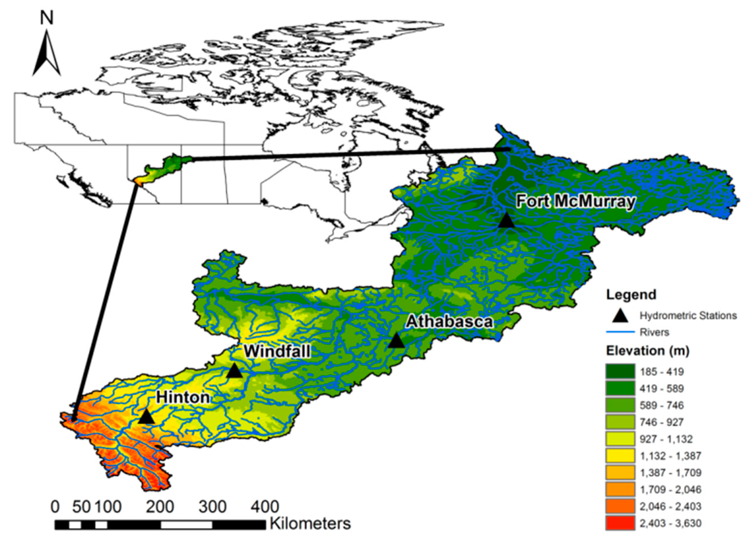
2.1. Study Area

The Athabasca River basin (ARB, see Figure 1) originates in the Canadian Rockies from the Athabasca Glacier, at over 3700 m above mean sea level (amsl), and flows approximately 1500 km north-eastward through the province of Alberta. It passes by, or through Jasper, Hinton, Whitecourt, Athabasca, and Fort McMurray, before emptying into Lake Athabasca (average elevation ~208 m amsl), which outflows through the Slave River and Lake to the Mackenzie River system. Its total drainage area attains approximately 156,000 km2 near Old Fort before it flows into Lake Athabasca. The watershed includes various land cover types, such as snow-capped mountains, agricultural plains, boreal forest, wetlands, and small urban areas. The boreal forest is dominated by coniferous followed by mixed and transitional forest. Mean annual precipitation in the watershed ranges from around 300 mm at the downstream end near Lake Athabasca to over 1000 mm at the high elevation head-waters. The region displays a typical nival hydrologic regime with low flows during the snow accumulation period of late autumn to early spring (November to March), and higher spring flows typically starting in April when air temperatures rise above freezing. The Athabasca River is ecologically and economically significant to the development and sustainability of northern Alberta with increasing population and industrial activities, including the multi-billion-dollar oil sands industry [26]. The quantity and quality of flow in the Athabasca River, including extreme high and low flow events, are essential in providing various ecosystem services in the river channels with implication to the downstream Peace Athabasca Delta, which is a UNESCO World Heritage Site and the largest freshwater inland river delta in North America [27].

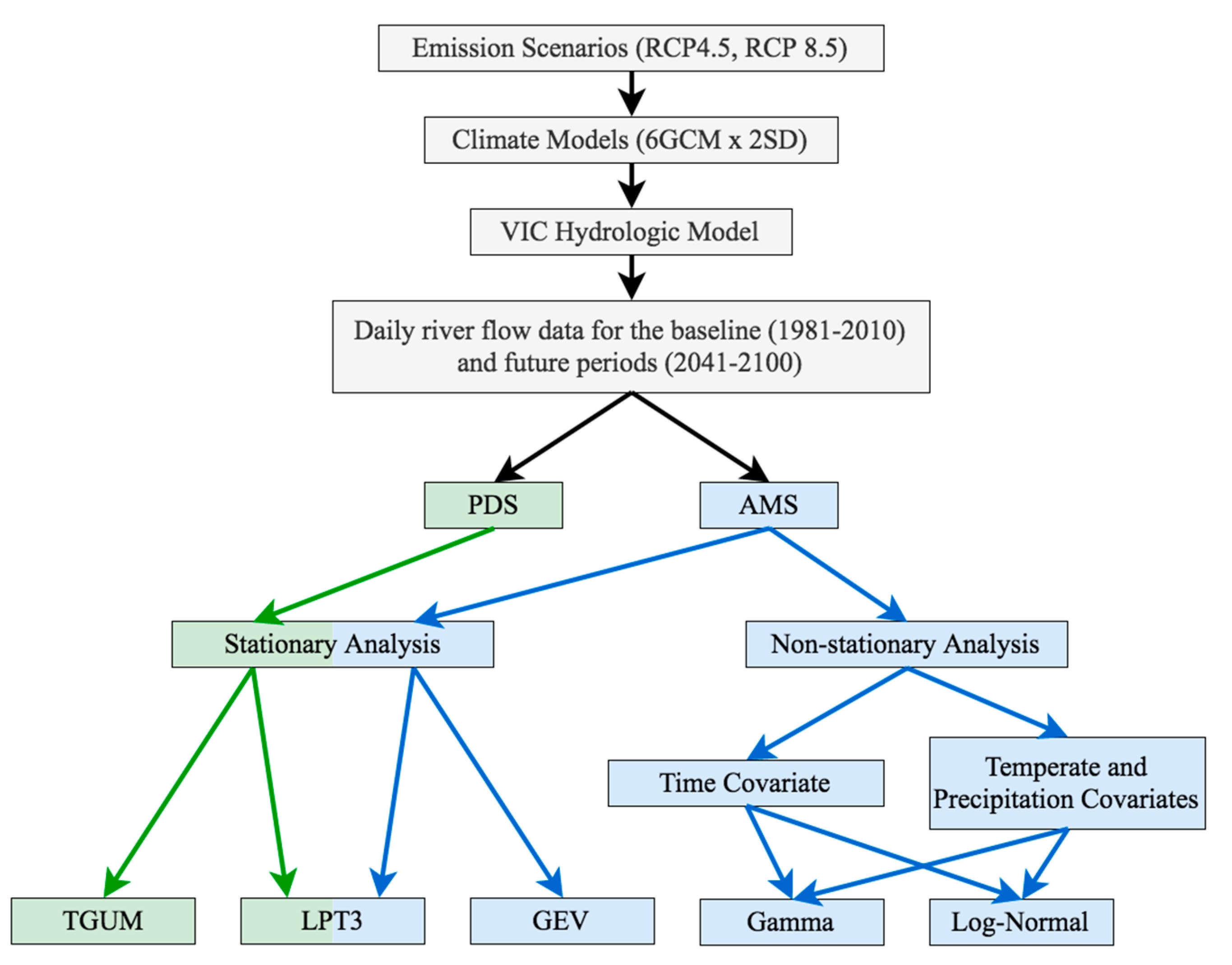
2.2. Climate Scenarios and Hydrologic Projections

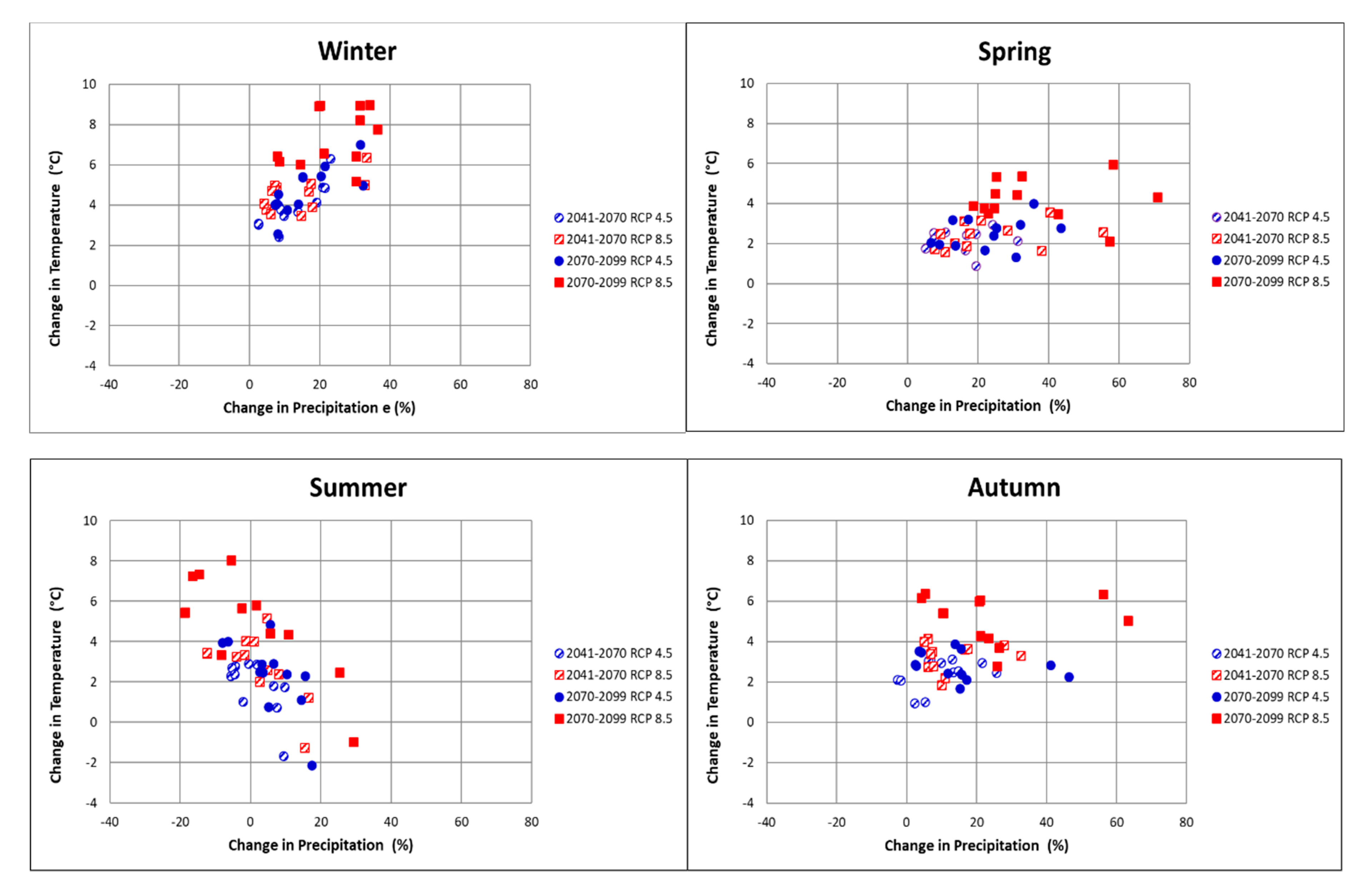
2.2.1. Climate Model Projection

Regional and local precipitation and potential evaporation are the main climatic drivers controlling the hydrology of a watershed system. A warming climate is shown to affect the magnitude and distribution of both temperature and precipitation that would, in turn, affect the water balance and hydrology of a region [28]. Therefore, studies on the potential impacts of climate change mostly rely on climate projections from global or regional climate models. This study employs statistically downscaled high-resolution gridded daily precipitation, as well as daily maximum (Tmax) and minimum (Tmin) air temperature data to drive a process-based and semi-distributed variable infiltration capacity (VIC) hydrologic model [29] to simulate hydrologic scenarios for the future period. The latest projections originate from twenty-six CMIP5 GCM long-term experimental runs corresponding to the four different levels of representative concentration pathways (RCP2.5, RCP4.5, RCP6.0, and RCP8.5) in which the labels of RCP represent an approximation of the radiative forcing in the year 2100 [30]. Climate projections corresponding to two of the four emission scenarios, namely, the RCP4.5, which is a stabilization scenario that achieve the goal of limiting emission and radiative forcings, and the RCP8.5, which is an emission scenario that greenhouse gas increases as usual until 2100, are selected for hydrologic modelling and analysis in this study. By applying a clustering approach and ranking the models, which differs by region, to provide the widest spread (range) in projected future climate for smaller subsets of the full ensemble, Cannon [31] suggested a set of representative GCMs that fully capture climate variability in 27 extreme climate indices. Moreover, Eum et al. [25] showed that selection of the top six GCMs for Western North America covers over 50% of the variations in the climatic indices considered for the Athabasca River basin. Therefore, the present study uses statistically downscaled data from six GCMs, corresponding to mid-range mitigation (RCP4.5) and high emissions (RCP8.5) scenarios that represent a wider range of climate extremes and seasonal means of precipitation and temperature (see Table 1). Murdock et al. [32] compared the skills of different statistical downscaling (SD) techniques based on sequencing, distribution and spatial pattern related indicators, and recommended two of the more reliable SD techniques, the Bias-Correction Spatial Downscaling (BCSD; [33]) and the bias correction/climate imprint (BCCI; [34]), for regional applications over Canada. The BCSD method uses a quantile-based mapping of the probability density functions for the monthly GCM precipitation and temperature onto those of a gridded observed data spatially aggregated to the GCM scale. Daily results at high spatial resolution are obtained by spatial and temporal disaggregation using rescaled randomly sampled historical observations. The BCCI method uses long-term averages (e.g., 30 years) from the high-resolution observational data as a ‘spatial imprint’ to represent spatial gradients. The ratio of daily GCM precipitation values to the long-term average monthly climatology of the baseline period is multiplied by the corresponding fine-scale monthly values for a location to get the daily precipitation. These two methods were applied to correct biases and downscale the daily precipitation, Tmax and Tmin scenario data covering the period 1951 to 2100 to a 10-km spatial resolution using the ANUSPLIN observation based gridded data for the 1951–2010 reference period [32]. A total of twenty-four climate projections, from six GCMs and two emission scenarios (RCP4.5 and RCP8.5) and downscaled with two statistical techniques (BCCI and BCSD), are employed to produce an ensemble of hydrologic projections for the Athabasca River basin [25]. This is because future projections by different GCMs usually diverge with time because of different initializations and representations of the various processes in the models and the rate of this divergence is higher for higher emissions scenarios.
Figure 2 shows the projected changes in seasonal mean precipitation and air temperature over the Athabasca River basin for the near future (2041–2070 or 2050s) and far future (2071–2100 or 2080s) periods relative to the baseline (1981–2010 or 1990s) period based on those multiple climate projections. The plots indicate overall increases in seasonal precipitation and air temperature over the region except in summer when some models projected decreases in precipitation. In general, the rate of increase in air temperature and precipitation is higher for the higher emission scenario (RCP8.5) compared to the medium RCP4.5 emission scenario and is also higher for the 2080s compared to the 2050s. In particular, there is a strong agreement among all the models with respect to pronounced projected increases in winter air temperature, ranging between 2.5 and 9 °C, and precipitation, ranging between 8% and 38% by the end of this century. At the same time, the ranges of climate projections for the RCP8.5/2080s scenario are found to be wider than those for the RCP4.5/2050s indicating that the inter-model variability in the climate projections gets larger with increasing emission concentrations and projection horizons. This is because future projections by different GCMs usually diverge with time because of differences in initial conditions and parameterizations of the various processes in the models and the rate of such divergence gets larger for higher emissions scenarios.

2.2.2. Hydrologic Modelling and River Flow Scenario Simulation

The variable infiltration capacity (VIC), land surface model, is a process-based and spatially distributed macro-scale hydrologic model that simulates the water and energy balances necessary to accurately account for cold-climate hydrologic processes based on prescribed land cover and three-soil layers [29]. The VIC hydrologic model has been successfully applied for evaluating the effects of climate change on hydrologic regimes for watersheds with different basin size, climatology and hydrologic processes [25,41,42]. The model has also been used for evaluation of historical flood events [43] and extreme flow projections [44,45] in several regions. However, one limitation of such hydrologic simulation of flow in cold region rivers is the assumption of open water flow throughout the year and not explicitly accounting for the effect of river-ice freeze-ups, ice-jam and break-up events. Eum et al. [25,46] applied the VIC model over the Athabasca watershed using daily precipitation and temperature data from the ANUSPLIN and statistically downscaled CMIP5 climate model projections. Receiving the daily Tmax, Tmin and Precipitation values, VIC is able to empirically estimate the other energy flux terms over the basin based on geographic coordinates and topographic information. The present study is based on the daily streamflow scenario simulated over the Athabasca watershed by Eum et al. [25] setup of the VIC hydrologic model, with specific emphasis on the analysis of potential changes in peak flows along the Athabasca River, due to projected climate.
The VIC hydrologic model calibration and validation for the Athabasca watershed were performed using daily discharge data at several hydrometric stations along the Athabasca River and its tributaries for the periods 1985–1997 and 1998–2010, respectively [25]. The performance of the calibrated VIC model in replicating the daily mean discharge at four of the hydrometric stations located along the Athabasca River mainstem and that are used for this study is summarized in Table 2. The results show Nash–Sutcliffe (NS) values for the calibration/ validation period ranging between 0.78/0.74 and 0.90/0.80. A more detailed description of the VIC model setup used for this study and its calibration/validation results can be found in Eum et al. [25,47].
The calibrated/validated VIC model is applied for hydrologic scenario simulations for the 1990s baseline, as well as for the near (2050s) and far (2080s) future periods, using the twelve sets of statistical downscaled high-resolution climate forcing, corresponding to both the RCP4.5 and RCP8.5 emissions scenarios. Figure 3 presents the box-and-whisker plot of mean monthly streamflow projections and the corresponding changes between the 1990s baseline and the future periods at two locations (a headwater station at Windfall and a downstream station below Fort McMurray) along the Athabasca River. The result indicates an overall projected increase in the Athabasca River discharge for most seasons except in the summer months of July, August, and September that show some decreases. The projected changes are also distinctively higher for the RCP8.5 emissions scenario during the far future period of the 2080s with the increase in mean annual flow ranging between 15.0% to 16.3% of the 1990s baseline value. The corresponding values for the RCP4.5 emissions scenario are relatively smaller, ranging between 7.2% to 11.7% [25].

2.3. Methods of Peak Flow Analysis

The primary objective of frequency analysis is to relate the magnitude of extreme events to their frequency of occurrence through the use of probability distribution [48]. Two different statistical models of analyzing peak flows, namely, AMS, and partial duration series (PDS) are employed in this study. AMS refers to a series of flow data consisting of the annual maximum daily streamflow values for each year. PDS, on the other hand, includes all independent peak flow events above some pre-defined threshold value. AMS is relatively simpler to apply, as it only requires selecting the annual maximum daily streamflow for analysis; however, some important episodes resulting from multiple independent peak flow events within a water year may be excluded from the study. The advantage of PDS is that it provides the possibility to control the number of flood occurrences to be included in the analysis by appropriate selection of the threshold. However, the choice of threshold and the selection of criteria for retaining flood peaks makes it difficult to use [49]. The specific threshold value for a PDS is usually decided after choosing the average annual number of peak flow events to be included in the PDS. To ensure the selected peak-flow events are independent, inter-event time criteria, specifying the minimum time interval between successive events, and an enter-event discharge level criteria, specifying the minimum flow level between successive events as a fraction of the smaller event, has to be set. After closer examination of the time series data, a minimum inter-even time interval of 72 h and an inter-event level fraction of 0.8 were used to extract the PDS from the daily time series data. This has resulted in 1 to 3 extreme events per year for most of the stations and ensemble members.
The AMS of simulated flows at each of the four hydrometric stations along the Athabasca River main steam corresponding to each of the 12 sets of climate projections (6 GCMs × 2 SD) are extracted for each of the two emission scenarios. A related issue to the magnitude of annual peak flows is the potential shift in the timing of these peak flow events. The Box-and-Whisker plots for the dates of the peak annual flow on Figure 4 show that the median date of AMS in the future scenarios will be getting earlier compared to the baseline period; and more so for the RCP8.5 scenario compared to the RCP4.5. This is an indication that future flooding season will probably shift to an earlier period by order of up to a month or more for the RCP8.5 scenario. Moreover, the variability in the dates of peak flow events will also increase substantially, indicating that the probability of mid-winter and early spring flooding will be increasing.

2.3.1. Stationary and Non-Stationary Analysis

Stationary flood frequency analysis assumes parameters of the probability distribution function for a given period to remain constant. Such analysis is performed in this study on both the AMS and PDS using the Extreme Value Analysis (EVA) tool under the MIKE-Zero platform [50]. Different combinations of six probability distributions (including Gumble, Truncated Gumbel (TGUM), Generalized Extreme Value (GEV), Weibull, Frechet, Log-Pearson Type 3 (LPT3)) and two estimation methods (Method of Moment (MOM) and Maximum Likelihood (ML)) were evaluated using the standardized least square measure and graphical comparison for fitting the observed peak flow data over the baseline period. While the AMS were best fitted with the LPT3 and the GEV distributions, the PDS were best fitted with LPT3 and TGUM distributions. The parameters for LPT3 distribution were estimated using the MOM, while the parameters for GEV and TGUM distributions were estimated using the ML method. The analysis is done over each of the three 30-year periods (centered at 1990s, 2050s, and 2080s) and the potential impacts of projected climate are estimated by computing the difference in the peak flow magnitudes of various return periods between the baseline and future periods.
However, in a non-stationary world, the probability density functions evolve dynamically over time. Hence, non-stationary analysis works by fitting data to a distribution where the location, scale and shape parameters can be functions of time or climatic variables such as temperature, precipitation or other influencing external factors, such as reservoir operation or land use changes [51]. The non-stationary analysis used in this study applies the generalized additive models for location, scale and shape (or GAMLSS; [52]) on the AMS data. GAMLSS is a general framework for fitting regression-based models that allow all the parameters of the distribution of the response variable to be modelled as linear/non-linear or smooth functions of the explanatory variables. In the present study, the response variable is a series of annual maximum peak discharge that has a parametric cumulative distribution function, and its parameters are modelled as a function of selected covariates. Several distributions under the R package of GAMLSS [53] were tested by modeling the parameters as a linear function of selected covariates and fitting them using the maximum likelihood estimation (MLE) method. Using the Akaike information criterion (AIC), the Schwarz Bayesian criterion (SBC) and by inspecting the quantiles of the residuals, the two parameters—gamma (GA) and log-normal (LNO) distributions—are identified to be most appropriate for the current study. First, time was used as the sole covariate and then annual precipitation and temperature are considered together as alternate covariates. For the latter case, mean annual temperature and annual total precipitation time series over each sub-watershed area contributing to each of the four hydrometric stations are calculated and used as covariates. As an example, Figure 5 presents a non-stationary LNO distribution fitted to simulated peak annual maximum flow series (AMS) at Fort McMurray station with the Log-Normal distribution parameters (µ and 𝛿) varying as a function of time (t). Once the best distribution parameters are fit as functions of the covariates, the projected changes in the frequency and magnitude of peak flow events are computed by averaging their corresponding values over each ten-year period in the 1990s, 2050s, and 2080s. Since there are twelve sets of simulated flow time series (6GCMs and 2DS) corresponding to each of the two emissions scenarios (RCP4.5 & 8.5), the projected changes are mostly reported as the ensemble mean values from all those simulations. The flowchart in Figure 6 illustrates all the different steps and combinations in model simulation, and statistical analysis of peak flows in the Athabasca River.

2.3.2. Uncertainty in Peak Flow Projections

The peak flow analysis in this study employs a set of daily streamflow time series simulated from the VIC hydrologic model of the Athabasca watershed forced with climate data from each of the twelve statistically downscaled GCMs (6GCMs × 2DS). Hence, the projected changes in the frequency of peak flows have a range of possible values resulting from the multiple simulations. In addition, both stationary and non-stationary analysis techniques are applied to each simulated streamflow time series, with different distribution functions and covariates, resulting in eight sets of outcomes for each streamflow projection. The sensitivity of projected changes in the frequency of peak flows to the driving climate models, as well as the statistical methods of analysis is examined by calculating the inter-climate model variability and the inter-statistical method variability in terms of their corresponding standard deviations. While inter-climate model standard deviation for each statistical method of frequency analysis is calculated from multiple projected changes corresponding to each climate models, inter-statistical model standard deviations corresponding to each driving climate model are calculated from projected changes by multiple statistical methods of analysis. Finally, the sensitivity of the projected change in peak flow to inter-climate model variability is compared with that of the inter-statistical method variability.

3. Results

3.1. Stationary Analysis

The stationary analysis techniques are applied on both the AMS and the PDS, at each of the four hydrometric stations along the Athabasca River. The time series of peak flow is derived from the VIC simulated streamflow data corresponding to each GCM, statistical downscaling (SD) methods and emissions scenario combination (RCPs). Analysis results are presented as peak flow magnitudes and corresponding changes for a number of events between 2- and a 100-year return periods. The results are then averaged over all the driving GCM/SD to create ensemble mean values for each future period and emissions scenario combination. Figure 7 shows the ensemble mean projected changes in peak flow events of different return periods between the 1990s baseline and the 2080s future periods corresponding to the RCP8.5 emissions scenario. The results indicate an overall decrease in the return period (or increase in the frequency) of most flow quantiles for the future period. At Fort McMurray, for instance, a 100-year peak flow event for the baseline period will become a 30-year one by the end of this century and a 50-year peak flow event will become more frequently than once in 20 years. Moreover, the average magnitudes of changes are relatively lower for the headwater stations at Hinton and Windfall compared to the downstream stations at Athabasca and Fort McMurray. Moreover, the ranges of predicted changes for the upstream stations are generally wider than those for the downstream stations indicating the increased uncertainty of the results for the upstream stations. Potential changes in the frequency of peak flow magnitudes, estimated using the AMS series are generally higher than those using the PDS. However, there seems to be no consistent pattern in the projected changes that can be attributable to the specific statistical methods applied to model the frequency distributions. The results corresponding to the RCP4.5 emission scenario (not presented) are very similar to that of the RCP8.5 except that the changes are relatively smaller for the former, with the 100-year peak flow at Fort McMurray becoming a 50-year one and a 50-year peak flow becoming a 30-year one by the end of the century.

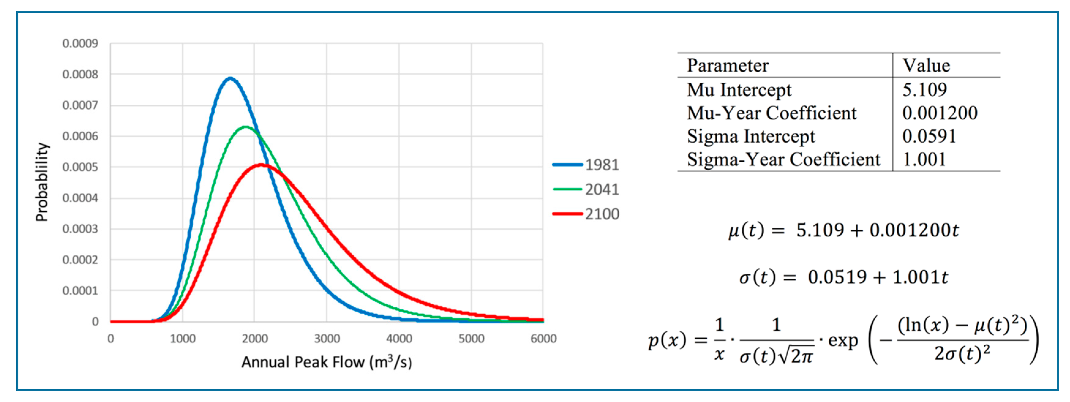
3.2. Non-Stationary Analysis

Non-stationary analysis on the AMS is performed first using time (as the number of years from the start of the AMS; i.e., 1981) as the only covariate and then using both the mean annual temperature and annual total precipitation as covariates on which the values of the distribution parameters for the Gamma and Log-Normal distributions depend. For each of the four hydrometric stations considered, the mean temperature and precipitation covariates are computed only over the region contributing (draining) to each of the measuring stations. As in Figure 7 and Figure 8 shows the ensemble mean projected changes in peak flow events of different return periods between the 1990s baseline and the 2080s future periods corresponding to the RCP8.5 emissions scenario. The magnitude and direction of changes in the ensemble mean results from the non-stationary analysis are generally similar to those of the stationary analysis for the two headwater stations (Hinton and Windfall) except that the ranges of the projected changes are narrower for the former. For the two downstream stations, however, the non-stationary analysis predicted greater changes (decreases) in the return periods of low frequency events than that of the stationary approach.
Moreover, using time as the only covariate predicted larger decreases in the return periods compared to using mean annual temperature and precipitation as covariates for the two upstream stations, while the reverse is true for the remaining two downstream stations (Athabasca and Fort McMurray). For example, a 100-year peak flow event for the baseline period will become a 35- to 62- year event at Hinton headwater station or a 15- to 22-year event at the downstream Fort McMurray station by the end of this century. When using precipitation and temperature as covariates, the Log-Normal distribution resulted in greater projected changes (decreases) in return periods compared to the Gama distribution. On the contrary, when using only time as a covariate, the Log-Normal distribution resulted in smaller projected changes (decreases) in return periods compared to the Gama distribution. Consistent with the case of the stationary analysis, the ranges of predicted changes for the upstream stations are generally wider than those for the downstream stations, again indicating the higher uncertainty in the results for the upstream stations.

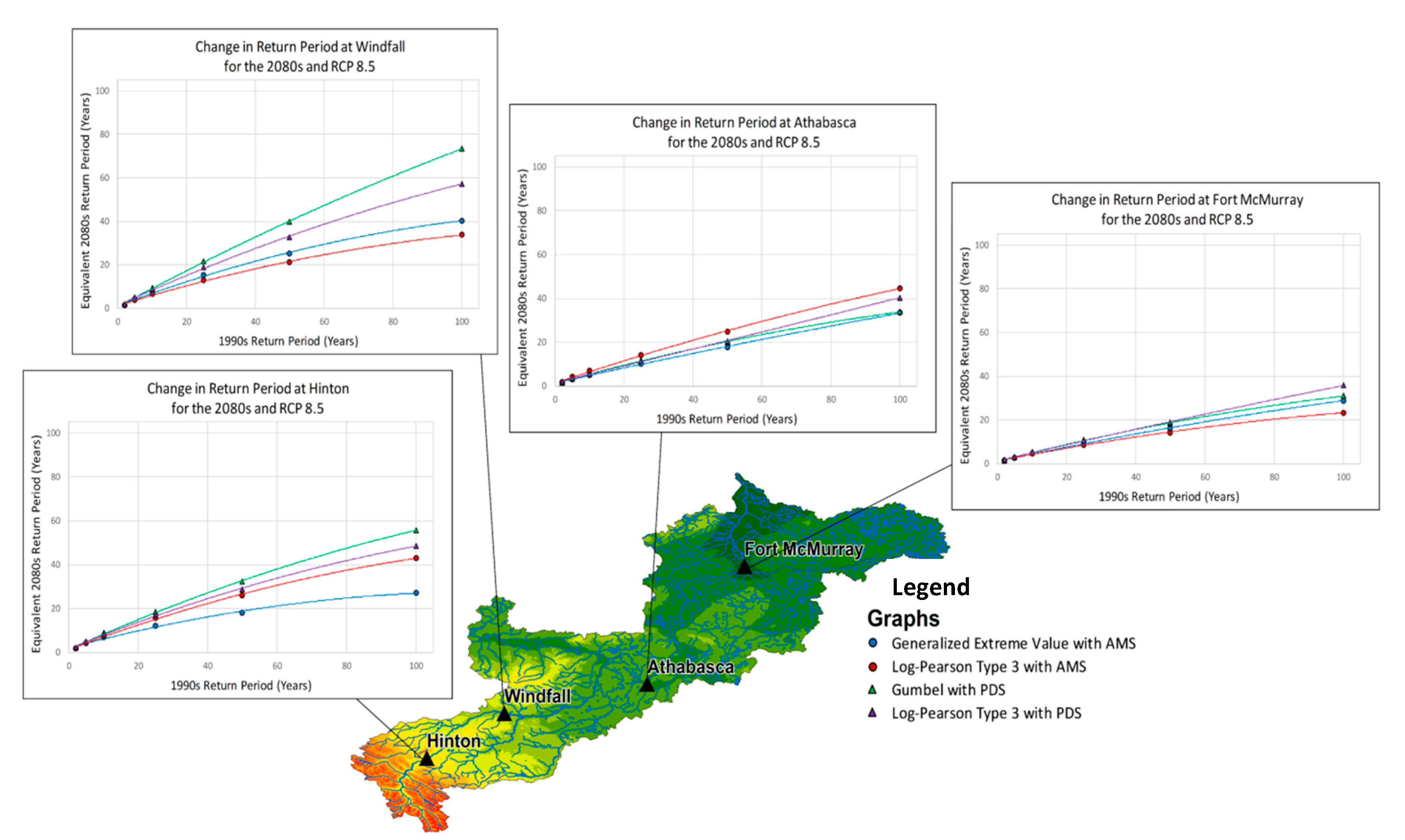
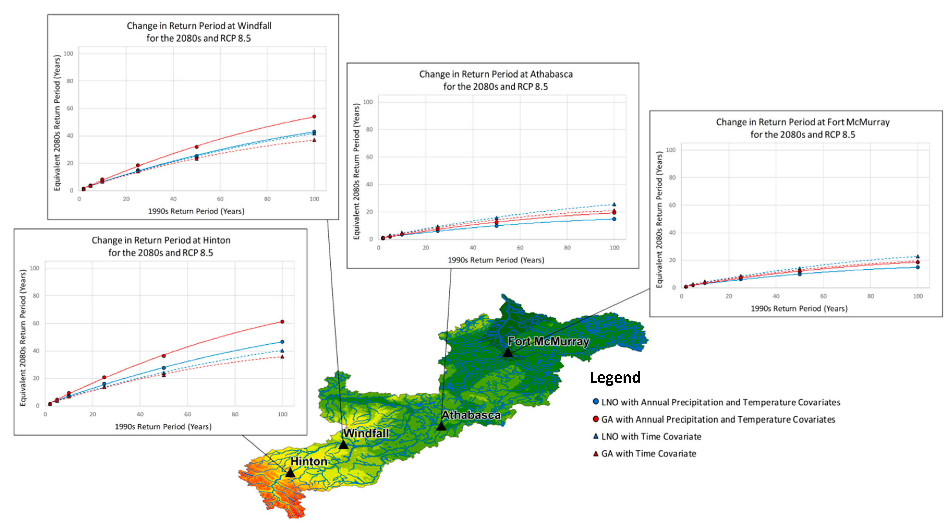
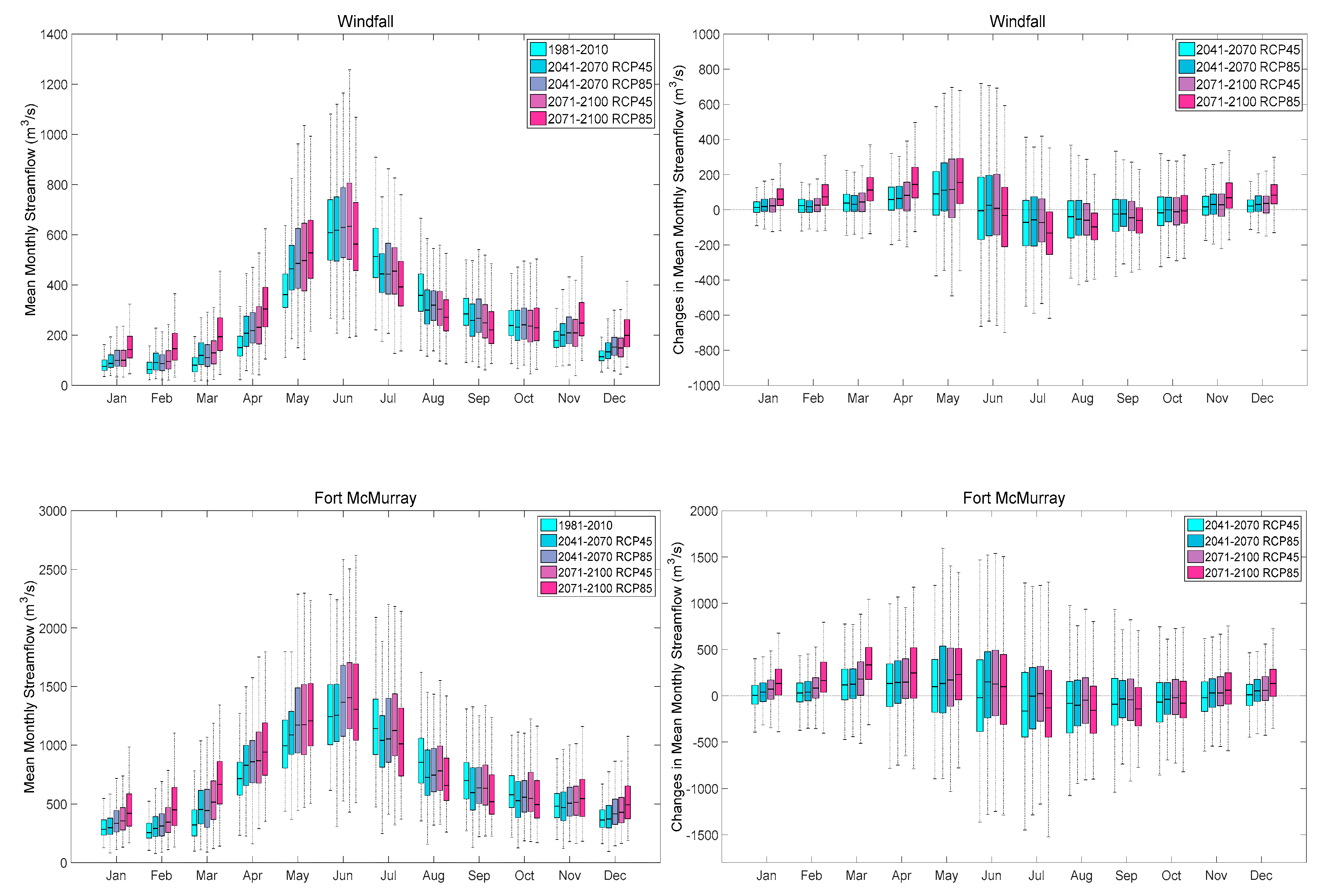
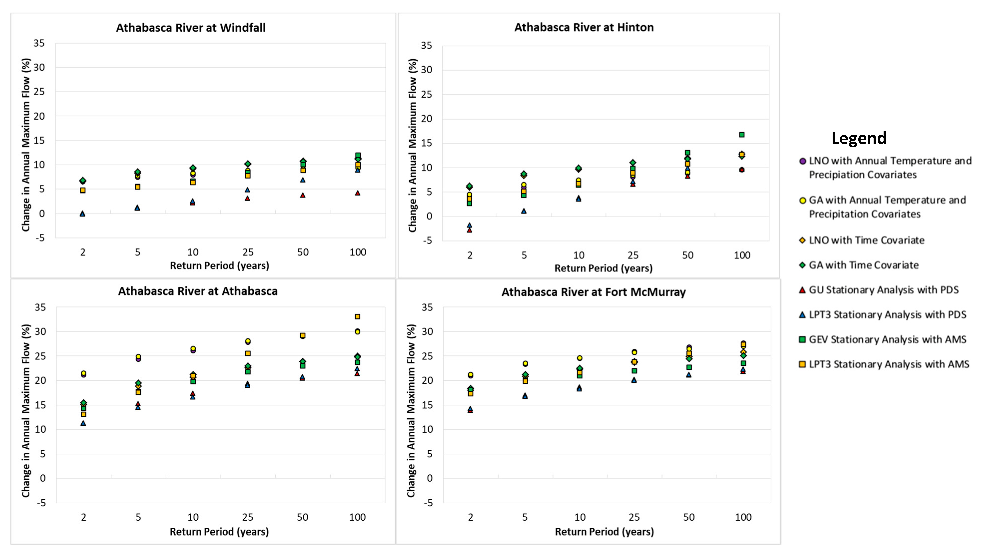
3.3. Changes in Peak Flows

Figure 9 presents the ensemble mean projected changes (%) in the magnitude of peak flow events of different return periods between the 2080s and the 1990s baseline period for the RCP8.5 emissions scenario based on both stationary and non-stationary methods of frequency analysis. The percentage of projected changes at each location varies depending on the statistical method of analysis, such as stationary vs non-stationary analysis, type of distribution function applied and the covariates used to model the parameters. The changes in the peak flow magnitudes generally get larger with increases in the return period. Relative changes at the downstream stations (Athabasca and Fort McMurray) are also generally higher than those at the headwater stations (Hinton and Windfall) resulting from accumulated effects of increasing flows within the drain area from the headwater to downstream stations. To show a specific example, peak flow events with a 100-year return period at the two upstream stations is projected to increases by about 4% to 12% during 2080s compared to the 1990s baseline period. The corresponding increases for the two downstream stations range from 21 to 33%. At the same time, the corresponding increases in peak flow events with 5-year return period at the two upstream stations vary from 1% to 9%, while it varies from 14% to 25% at the two downstream stations. Similar increases in peak flow magnitude are projected for the RCP4.5 emissions scenarios; however, the changes are slightly smaller with projected increases in the 100-year peak flow at the two downstream stations varying from 18% to 28% (not shown).
The non-stationary analysis mostly results in greater projected changes in peak flows than the stationary ones. The smallest relative changes resulted from the stationary analysis performed on the PDS data, while non-stationary analysis with AMS and using precipitation and temperature as covariate resulted in the biggest projected changes. For example, while stationary analysis performed on the PDS at each of the four stations resulted in 4% to 23% increases in the 100-year peak flow event by the 2080s, compared to the 1990s, the corresponding increase for non-stationary analysis with AMS using precipitation and temperature as covariate range between 10% to 30%.

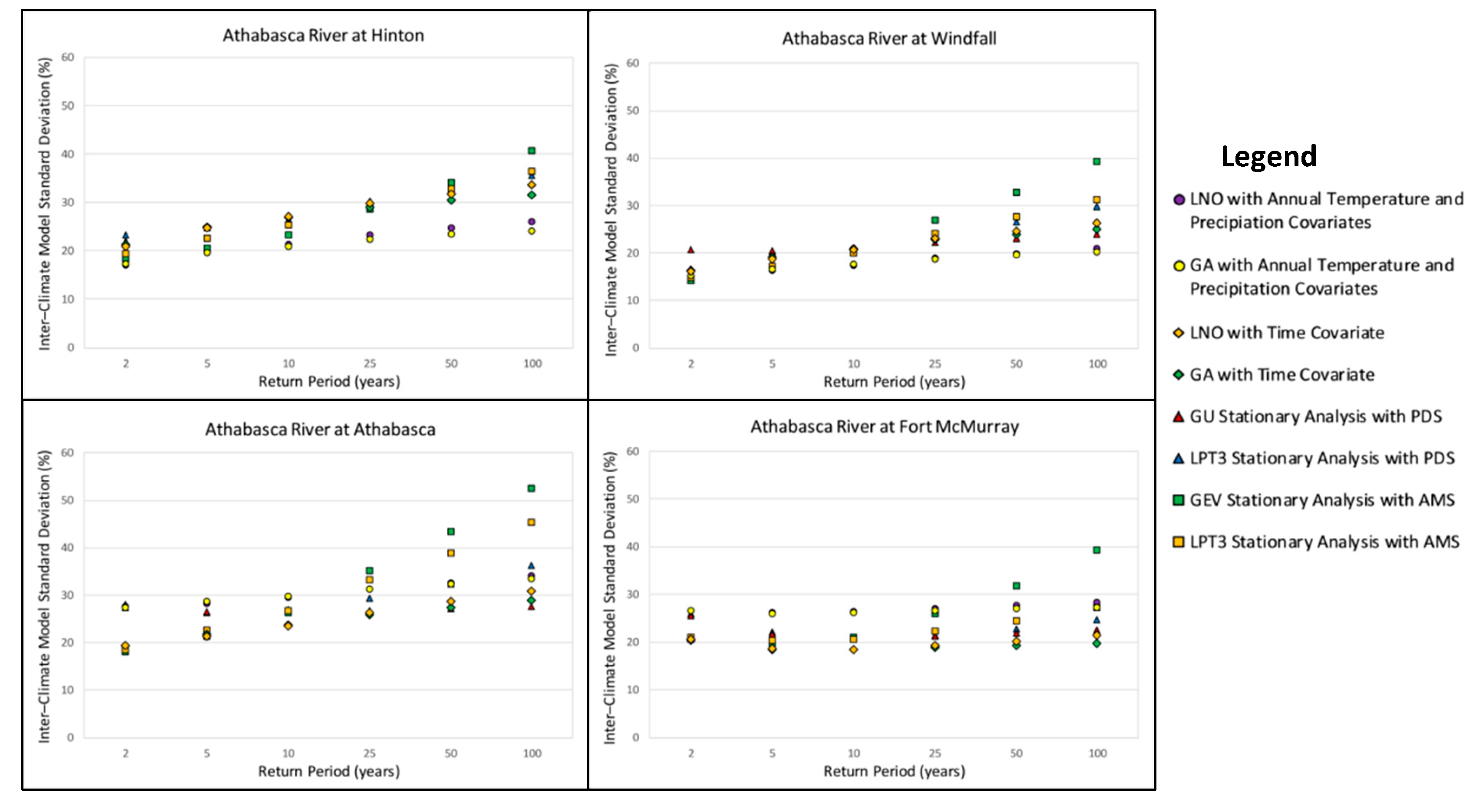
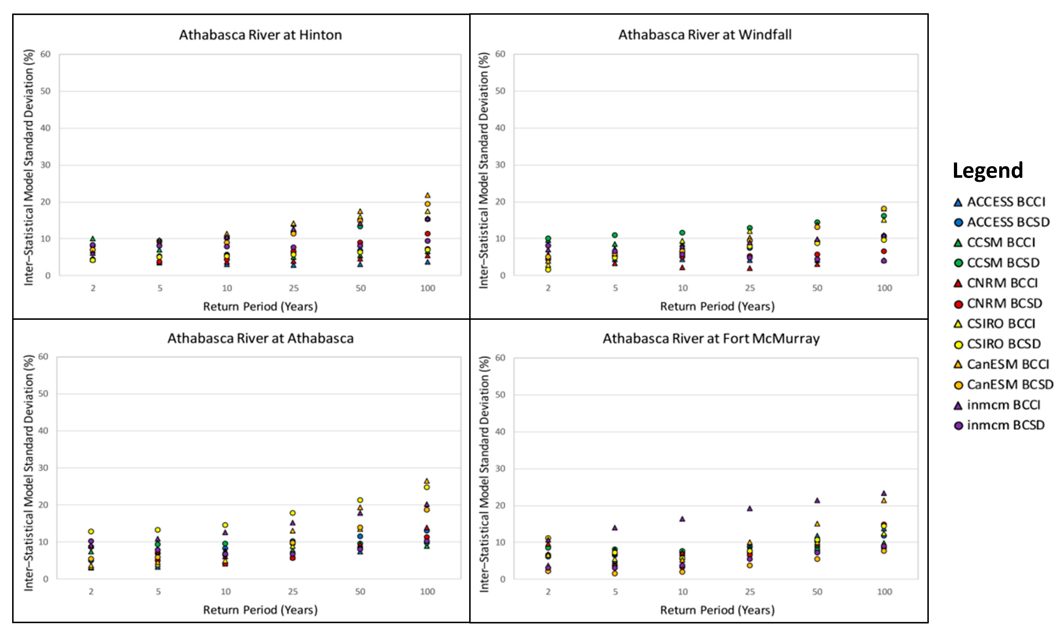
3.4. Inter-Model Variability

The analysis results presented above show that projected changes in the magnitude and frequency of peak flow results for a given emission scenario and future horizon depends on both the climate models corresponding to the streamflow projection and the statistical method of frequency analysis. Inter-climate model variability of projected changes in peak flow corresponding to each method of extreme flow analysis is presented in Figure 10. The result shows the inter-climate model standard deviation of the changes between the 2080s and the 1990s baseline period and the RCP8.5 emissions scenario for a range of return periods. The inter-climate model variability in projected changes is generally larger as the return period gets longer. For example, while the ensemble mean value of projected changes in the 100-year peak flow at the Fort McMurray station range between 22% and 28%, its standard deviation range between 19% and 39% depending on the statistical method of analysis. While the stationary analysis with AMS produces the greatest inter-climate model variability, the non-stationary analysis with precipitation and temperature co-variate generally produces the smallest inter-climate model variability. This is an indication that the uncertainty in the parameters of the frequency distributions is reduced by using the driving temperature and precipitation as co-variates to constrain their values. There seems to be no systematic difference in the pattern of inter-climate model variability between the different stations.
Figure 11 presents the inter-statistical model variability of projected changes in peak flow between the 2080s and the 1990s baseline period and the RCP8.5 emissions scenario for each of the climate models considered. The inter-statistical model standard deviation of projected changes shows a similar pattern at all the four stations with a gradual increase with an increase in the return period. For example, the inter-statistical model variation in the 100-year peak flow at the Fort McMurray station ranges between 7% and 24% depending on the climate model employed. While there are different patterns of inter-statistical model variabilities corresponding to each of the climate models, the ranges of variabilities are very similar with slightly higher values and wider ranges for higher return periods. However, when compared to the inter-climate model standard deviation, the inter-statistical model standard deviations are generally smaller, indicating that the uncertainty in projected changes resulting from the driving climate models is generally higher than that coming from the statistical methods of extreme flow analysis.

4. Summary and Conclusions

The study examines potential changes in the frequency and magnitude of peak flows in the Athabasca River in Alberta, Canada based on simulated discharges for the future climate. The daily stream flows for the baseline and future periods are simulated with the VIC hydrological model of the Athabasca watershed driven by multiple statistically-downscaled high-resolution climate scenarios corresponding to the RCP4.5 and RCP8.5 emissions scenarios. Analysis of simulated flows generally indicates potential increases during the winter and spring and decreases during the summer and early fall seasons, with an overall increase in high flows, especially for low frequency peak flow events. However, the study also reveals that projected changes in the frequency and magnitude of peak flow events vary over a wide range, especially for low frequency events, depending on the climate model/data used to simulate the streamflow and the statistical method of peak flow analysis. For example, the ensemble mean projected changes for the 100-year peak flow event by 2080s ranges from 4% to 33% depending on emissions scenarios and the statistical method of analysis. These increases correspond to a 100-year peak flow event of the 1990s baseline period becoming a 20- to 50-year event at the end of the current century with larger changes at downstream stations compared to upstream ones. While all peak flows may not necessarily cause flooding, the projected increase in the frequency and magnitude of future peak flow events are most likely to increase the probability of flooding in specific reaches (with floodplain) along the river.
The non-stationary peak flow analyses show relatively larger increases in peak flow magnitudes at different return periods compared to that of the stationary methods, especially for the downstream stations. The stationary analysis on the PDS resulted in smaller projected changes in peak flows than that of the AMS. However, the application of stationary analysis over multiple 30-years epochs as compared to a combined 90 years of data for the non-stationary analysis may have some bearing on the comparison two approaches. The two non-stationary approaches, one using time as the only covariate, and the other using precipitation and temperature as covariates, have also produced slightly different results that can be explained by the nature of the covariates. With only time as a covariate, the changes in the model parameters are linear, while using the temperature and precipitation covariates, the changes in the model parameters are non-linear as they depend on the variation in temperature and precipitation. This seems to allow the multivariate analysis, with temperature and precipitation as covariates, to fit better to the changing frequency of peak flows. The effect of the distribution applied (log-normal vs gamma) on the magnitude of the changes is also found to be different depending on the covariates employed and no specific distribution seems to produce the consistently higher or lower magnitude of changes for all the different cases. The study also showed that inter-model variabilities generally increase with increases in the return periods, mostly because there is an increasing reliance on distribution characteristics for predicting less frequent events. In general, the projected changes in the frequency and magnitude of peak flow events vary depending on both the driving GCMs and the statistical methods of peak flow analysis. However, the sensitivity of changes to the statistical method of analysis is generally smaller compared to that resulting from inter-climate model variability. Therefore, while the issue of non-stationarity is important in future peak flow projection, considering the range of model projections for the future climate condition is equally or even more important.

Author Contributions

Conceptualization, Y.D., H-I.E. and P.C.; methodology, Y.D., H-I.E. and J.H..; investigation and analysis, Y.D and J.H.; writing—original draft preparation, Y.D and J.H.; writing—review and editing, P.C. and H-I.E.; project administration, Y.D.; funding acquisition, Y.D.”

Funding

This study was conducted with the financial support provided by the Environment and Climate Change Canada’s Climate Change Adaptation program and the Joint Oil-Sands Monitoring Program (JOSMP).

Acknowledgments

This project was conducted in collaboration with the NSERC funded Canadian FloodNet project. The authors also acknowledge the contribution of Émilie Wong and Victoria Gagnon at the various stages of data acquisition and processing.

Conflicts of Interest

The authors declare no conflict of interest.

References

  1. Cunderlik, J.M.; Ouarda, T.B.M.J. Trends in the timing and magnitude of floods in Canada. J. Hydrol. 2009, 375, 471–480. [Google Scholar] [CrossRef]
  2. Park, D.; Markus, M. Analysis of a changing hydrologic flood regime using the Variable Infiltration Capacity model. J. Hydrol. 2014, 515, 267–280. [Google Scholar] [CrossRef]
  3. Buttle, J.M.; Allen, D.M.; Caissie, D.; Davison, B.; Hayashi, M.; Peters, D.L.; Pomeroy, J.W.; Simonovic, S.; St-Hilaire, A.; Whitfield, P.H. Flood processes in Canada: regional and special aspects. Can. Water Resour. J. 2016, 41, 7–30. [Google Scholar] [CrossRef]
  4. Beltaos, S.; Prowse, T. River-ice hydrology in a shrinking cryosphere. Hydrol. Process. 2009, 23, 122–144. [Google Scholar] [CrossRef]
  5. Prowse, T.D.; Beltaos, S. Climatic control of river-ice hydrology: a review. Hydrol. Process. 2002, 16, 805–822. [Google Scholar] [CrossRef]
  6. Burn, D.H.; Sharif, M.; Zhang, K. Detection of trends in hydrological extremes for Canadian watersheds. Hydrol. Process. 2010, 24, 1781–1790. [Google Scholar] [CrossRef]
  7. Ganguli, P.; Coulibaly, P. Does nonstationarity in rainfall require nonstationary intensity–duration–frequency curves? Hydrol. Earth Syst. Sci. 2017, 21, 6461–6483. [Google Scholar] [CrossRef]
  8. Burn, D.H. Climatic influences on streamflow timing in the headwaters of the Mackenzie River Basin. J. Hydrol. 2008, 352, 225–238. [Google Scholar] [CrossRef]
  9. Rao, A.R.; Hamed, K.H. Flood Frequency Analysis; CRC press: New York, NY, USA, 2000. [Google Scholar]
  10. Cooley, D. Return periods and return levels under climate change. In Extremes in a Changing Climate; AghaKouchak, A., Easterling, D., Hsu, K., Sorooshian, S., Eds.; Springer: Dordrecht, The Netherlands, 2013; Volume 65, pp. 97–114. [Google Scholar]
  11. Tramblay, Y.; Neppel, L.; Carreau, J.; Najib, K. Non-stationary frequency analysis of heavy rainfall events in southern France. Hydrol. Sci. J. 2013, 58, 280–294. [Google Scholar] [CrossRef]
  12. Khaliq, M.N.; Ouarda, T.B.M.J.; Ondo, J.C.; Gachon, P.; Bob´ee, B. Frequency analysis of a sequence of dependent and/or non-stationary hydro-meteorological observations: A review. J. Hydrol. 2006, 329, 534–552. [Google Scholar] [CrossRef]
  13. Cunderlik, J.M.; Burn, D.H. Non-stationary pooled flood frequency analysis. J. Hydrol. 2003, 276, 210–223. [Google Scholar] [CrossRef]
  14. Tan, X.; Gan, T.Y. Nonstationary analysis of annual maximum streamflow of Canada. J. Clim. 2015, 28, 1788–1805. [Google Scholar] [CrossRef]
  15. Ouarda, T.B.M.J.; El-Adlouni, S. Bayesian nonstationary frequency analysis of hydrological variables 1. JAWRA 2011, 47, 496–505. [Google Scholar]
  16. López, J.; Francés, F. Non-stationary flood frequency analysis in continental Spanish rivers, using climate and reservoir indices as external covariates. Hydrol. Earth Syst. Sci. 2013, 17, 3189–3203. [Google Scholar] [CrossRef] [Green Version]
  17. Li, J.; Tan, S. Nonstationary flood frequency analysis for annual flood peak series, adopting climate indices and check dam index as covariates. Water Resour. Manag. 2015, 29, 5533–5550. [Google Scholar] [CrossRef]
  18. Seidou, O.; Ramsay, A.; Nistor, I. Climate change impacts on extreme floods I: combining imperfect deterministic simulations and non-stationary frequency analysis. Nat. Hazards 2012, 61, 647–659. [Google Scholar] [CrossRef]
  19. Zhang, T.; Wang, Y.; Wang, B.; Tan, S.; Feng, P. Nonstationary flood frequency analysis using univariate and bivariate time-varying models based on GAMLSS. Water 2018, 10, 819. [Google Scholar] [CrossRef]
  20. Dong, N.D.; Agilan, V.; Jayakumar, K.V. Bivariate Flood Frequency Analysis of Nonstationary Flood Characteristics. J. Hydrol. Eng. 2019, 24, 04019007. [Google Scholar] [CrossRef]
  21. Shrestha, R.R.; Cannon, A.J.; Schnorbus, M.A.; Zwiers, F.W. Projecting future nonstationary extreme streamflow for the Fraser River, Canada. Clim. Chang. 2017, 145, 289–303. [Google Scholar] [CrossRef]
  22. Bonsal, B.R.; Cuell, C. Hydro-climatic variability and extremes over the Athabasca River basin: Historical trends and projected future occurrence. Can. Water Resour. J. 2017, 42, 315–335. [Google Scholar] [CrossRef]
  23. Dibike, Y.; Prowse, T.; Bonsal, B.; O’Neil, H. Implications of future climate on water availability in the western Canadian river basins. Int. J. Clim. 2017, 37, 3247–3263. [Google Scholar] [CrossRef]
  24. Dibike, Y.; Eum, H.I.; Prowse, T. Modelling the Athabasca watershed snow response to a changing climate. J. Hydrol. Reg. Stud. 2018, 15, 134–148. [Google Scholar] [CrossRef]
  25. Eum, H.I.; Dibike, Y.; Prowse, T. Climate-induced alteration of hydrologic indicators in the Athabasca River Basin, Alberta, Canada. J. Hydrol. 2017, 544, 327–342. [Google Scholar] [CrossRef]
  26. Rogers, M.E. Surface Oil Sands Water Management Summary Report; Cumulative Environmental Management Association (CEMA): Fort McMurray, AB, Canada, 2010. [Google Scholar]
  27. Prowse, T.D.; Beltaos, S.; Gardner, J.T.; Gibson, J.J.; Granger, R.J.; Leconte, R.; Peters, D.L.; Pietroniro, A.; Romolo, L.A.; Toth, B. Climate change, flow regulation and land-use effects on the hydrology of the Peace-Athabasca-Slave system; Findings from the Northern Rivers Ecosystem Initiative. Environ. Monit. Assess. 2006, 113, 167–197. [Google Scholar] [CrossRef] [PubMed]
  28. Stocker, T.; Qin, D. (Eds.) Climate Change 2013: The Physical Science Basis: Working Group I Contribution to the Fifth Assessment Report of the Intergovernmental Panel on Climate Change; Cambridge University Press: New York, NY, USA, 2014. [Google Scholar]
  29. Liang, X. A Two-Layer Variable Infiltration Capacity Land Surface Representation for General Circulation Models. Ph.D. Dissertation, NASA, Washington, DC, USA, 1994. [Google Scholar]
  30. Taylor, K.E.; Stouffer, R.J.; Meehl, G.A. An overview of CMIP5 and the experiment design. Bull. Am. Meteorol. Soc. 2012, 93, 485–498. [Google Scholar] [CrossRef]
  31. Cannon, A.J. Selecting GCM scenarios that span the range of changes in a multimodel ensemble: application to CMIP5 climate extremes indices. J. Clim. 2015, 28, 1260–1267. [Google Scholar] [CrossRef]
  32. Murdock, T.Q.; Cannon, A.J.; Sobie, S.R. Statistical Downscaling of Future Climate Projections; Pacific Climate Impacts Consortium (PCIC): Victoria, BC, Canada, 2013. [Google Scholar]
  33. Maurer, E.P.; Hidalgo, H.G. Utility of daily vs. monthly large-scale climate data: an intercomparison of two statistical downscaling methods. Hydrol. Earth Syst. Sci. 2008, 12, 551–563. [Google Scholar] [CrossRef] [Green Version]
  34. Hunter, R.D.; Meentemeyer, R.K. Climatologically aided mapping of daily precipitation and temperature. J. Appl. Meteorol. 2005, 44, 1501–1510. [Google Scholar] [CrossRef]
  35. Voldoire, A.; Sanchez-Gomez, E.; Mélia, D.S.; Decharme, B.; Cassou, C.; Sénési, S.; Valcke, S.; Beau, I.; Alias, A.; Chevallier, M.; et al. The CNRM-CM5.1 global climate model: description and basic evaluation. Clim. Dyn. 2013, 40, 2091–2121. [Google Scholar] [CrossRef]
  36. Arora, V.K.; Scinocca, J.F.; Boer, G.J.; Christian, J.R.; Denman, K.L.; Flato, G.M.; Kharin, V.V.; Lee, W.S.; Merryfield, W.J. Carbon emission limits required to satisfy future representative concentration pathway of greenhouse gases. Geophys. Res. Lett. 2011, 38, L05805. [Google Scholar] [CrossRef]
  37. Marsland, S.J.; Bi, D.; Uotila, P.; Fiedler, R.; Griffies, S.M.; Lorbacher, K.; O’Farrell, S.; Sullivan, A.; Uhe, P.; Zhou, X.; et al. Evaluation of ACCESS climate model ocean diagnostics in CMIP5 simulations. Austral. Meteorol. Oceanogr. J. 2013, 63, 101–119. [Google Scholar] [CrossRef]
  38. Volodin, E.M.; Dianskii, N.A.; Gusev, A.V. Simulating present-day climate with the INMCM4.0 coupled model of the atmospheric and oceanic general circulations. Izv. Atmos. Ocean. Phys. 2010, 46, 414–431. [Google Scholar] [CrossRef]
  39. Jeffrey, S.J.; Rotstayn, L.D.; Collier, M.A.; Dravitzki, S.M.; Hamalainen, C.; Moeseneder, C.; Wong, K.K.; Syktus, J.I. Australia’s CMIP5 submission using the CSIRO Mk3.6 model. Austral. Meteorol. Oceanogr. J. 2013, 63, 1–13. [Google Scholar] [CrossRef]
  40. Gent, P.R.; Danabasoglu, G.; Donner, L.J.; Holland, M.M.; Hunke, E.C.; Jayne, S.R.; Lawrence, D.M.; Neale, R.B.; Rasch, P.J.; Vertenstein, M.; et al. The community climate system model version 4. J. Clim. 2011, 24, 4973–4991. [Google Scholar] [CrossRef]
  41. Werner, A.T.; Schnorbus, M.A.; Shrestha, R.R.; Eckstrand, H.D. Spatial and temporal change in the hydro-climatology of the Canadian portion of the Columbia River basin under multiple emissions scenarios. Atmos. Ocean. 2013, 51, 357–379. [Google Scholar] [CrossRef]
  42. Elsner, M.M.; Cuo, L.; Voisin, N.; Deems, J.S.; Hamlet, A.F.; Vano, J.A.; Mickelson, K.E.; Lee, S.Y.; Lettenmaier, D.P. Implications of 21st century climate change for the hydrology of Washington State. Clim. Chang. 2010, 102, 225–260. [Google Scholar] [CrossRef] [Green Version]
  43. Wenger, S.J.; Luce, C.H.; Hamlet, A.F.; Isaak, D.J.; Neville, H.M. Macroscale hydrologic modeling of ecologically relevant flow metrics. Water Resour. Res. 2010, 46, W09513. [Google Scholar] [CrossRef]
  44. Västilä, K.; Kummu, M.; Sangmanee, C.; Chinvanno, S. Modelling climate change impacts on the flood pulse in the Lower Mekong floodplains. J. Water Clim. Chang. 2010, 1, 67–86. [Google Scholar] [CrossRef]
  45. Hamlet, A.F.; Lettenmaier, D.P. Effects of 20th century warming and climate variability on flood risk in the western US. Water Resour. Res. 2007, 43. [Google Scholar] [CrossRef]
  46. Eum, H.I.; Dibike, Y.; Prowse, T. Comparative evaluation of the effects of climate and land-cover changes on hydrologic responses of the Muskeg River, Alberta, Canada. J. Hydrol. Reg. Stud. 2016, 8, 198–221. [Google Scholar] [CrossRef] [Green Version]
  47. Eum, H.I.; Yonas, D.; Prowse, T. Uncertainty in modelling the hydrologic responses of a large watershed: a case study of the Athabasca River Basin, Canada. Hydrol. Process. 2014, 28, 4272–4293. [Google Scholar] [CrossRef]
  48. Chow, V.T.; Maidment, D.R.; Mays, L.W. Applied Hydrology; Editions McGraw-Hill: New York, NY, USA, 1988; 572p. [Google Scholar]
  49. Lang, M.; Ouarda, T.B.M.J.; Bobée, B. Towards operational guidelines for over-threshold modeling. J. Hydrol. 1999, 225, 103–117. [Google Scholar] [CrossRef]
  50. DHI. Extreme Value Analysis (EVA) Technical Reference and Documentation. 2017. Available online: manuals.mikepoweredbydhi.help/2017/General/EVA_SciDoc.pdf (accessed on 12 June 2019).
  51. Salvadori, G.; De Michele, C. Multivariate extreme value methods. In Extreme in a Changing Climate; Springer: Dordrecht, The Netherlands, 2013; pp. 115–162. [Google Scholar]
  52. Rigby, R.A.; Stasinopoulos, D.M. Generalized additive models for location, scale and shape. J. R. Stat. Soc. Ser. C (Appl. Stat.) 2005, 54, 507–554. [Google Scholar] [CrossRef]
  53. Stasinopoulos, M.D.; Rigby, R.A.; Heller, G.Z.; Voudouris, V.; De Bastiani, F. Flexible Regression and Smoothing: Using GAMLSS in R; Chapman and Hall/CRC: Boca Raton, FL, USA, 2017. [Google Scholar]
Figure 1. Athabasca watershed with its elevation range and the Athabasca River network, including the locations of the four hydrometric stations used for flood frequency analysis.
Climate 07 00088 g001
Figure 2. Projected changes in seasonal mean precipitation and air temperature over the Athabasca watershed.
Climate 07 00088 g002
Figure 3. Box-and-Whisker plot of mean monthly streamflow projections and the corresponding changes between the baseline (1990s) and two future periods (2050s and 2080s) at two locations along the Athabasca River based on 12 sets of climate projections (six GCMs × 2 SD) and two RCPs (RCP4.5 and RCP8.5).
Climate 07 00088 g003
Figure 4. Box-and-Whisker plots of the dates of annual maximum flow series (AMS) corresponding to the two emissions scenario (RCP4.5 and RCP8.5) as simulated at each of the four hydrometric stations along the Athabasca River for the baseline (1990s, blue) and the two future periods (2050s (green) and 2080s (red)).
Climate 07 00088 g004
Figure 5. Illustration of a non-stationary LNO distribution fitted to simulated AMS at Fort McMurray station with distribution parameters varying as a function of time (t).
Climate 07 00088 g005
Figure 6. General flowchart showing all the different steps and combinations in hydrologic model simulation and statistical analysis of peak flows in the Athabasca River. GEV, generalized extreme value; PDS, partial duration series; LPT3, log-Pearson type 3; TGUM, Truncated Gumbel.
Climate 07 00088 g006
Figure 7. Results of stationary analysis - ensemble mean projected changes in flood events of different return periods between the 1990s baseline and the 2080s future periods corresponding to the RCP8.5 emissions scenario.
Climate 07 00088 g007
Figure 8. Results of non-stationary analysis - ensemble projected changes in flood events of different return periods corresponding to the 1990s baseline and the 2080s future periods corresponding to the RCP8.5 emissions scenarios. The analysis is conducted on AMS using time, as well as temperature and precipitation covariates.
Climate 07 00088 g008
Figure 9. Ensemble mean projected changes (%) in the magnitude of flood events of different return periods between the 2080s and the 1990s baseline period for the RCP8.5 emissions scenario corresponding to both stationary and non-stationary methods of extreme flow analysis.
Climate 07 00088 g009
Figure 10. Inter- climate model variability of projected changes in peak flow between the 2080s and the 1990s baseline period for the RCP8.5 emissions scenario corresponding to each of the statistical methods considered.
Climate 07 00088 g010
Figure 11. Inter-statistical model variability of projected changes in peak flow between the 2080s and the 1990s baseline period and the RCP8.5 emissions scenario corresponding to each of the GCM/SD considered.
Climate 07 00088 g011
Table 1. The select set of six Global Climate Models (GCMs) from the coupled model inter-comparison project (CMIP5) experiment employed in this study.
GCM
Abbreviation
InstitutionResolution
(Lon. × Lat.)
Primary Reference
CNRM-CM5.1Centre National de Recherches Meteorologiques and Cerfacs1.4 × 1.4Voldoire et al. [35]
CanESM2Canadian Centre for Climate Modelling and Analysis2.8 × 2.8Arora et al. [36]
ACCESS1Centre for Australian Weather and Climate Research1.875 × 1.25Marsland et al. [37]
INM-CM4Institute of Numerical Mathematics2.00 × 1.50Volodin et al. [38]
CSIRO-Mk3.6.0Commonwealth Scientific and Industrial Re search Organisation1.875 × 1.86Jeffrey et al. [39]
CCSM4National Center for Atmospheric Research (NCAR)1.25 × 0.94Gent et al. [40]
Table 2. The VIC hydrologic model performances in terms of the Nash–Sutcliffe values during the calibration (1985−1997) and validation (1998−2010) periods.
StationHintonWindfallAthabascaFt.McMurray
Calibration0.900.810.780.79
Validation0.780.800.750.74

