Article

Impacts of Climate Change and Urban Expansion on Hydrologic Ecosystem Services in the Milwaukee River Basin

Department of Geography, University of Wisconsin-Milwaukee, Milwaukee, WI 53201, USA
*
Author to whom correspondence should be addressed.
Climate 2019, 7(4), 59; https://doi.org/10.3390/cli7040059
Submission received: 27 February 2019 / Revised: 12 April 2019 / Accepted: 18 April 2019 / Published: 20 April 2019
(This article belongs to the Special Issue Climate Change Resilience and Urban Sustainability)

Abstract

:
Land use/land cover (LULC) and climate changes could affect water quantity and quality and thus hydrologic ecosystem services (ES). However, studies of these impacts on hydrologic ES are limited by the current methods and techniques. We attempted to find out how the LULC and climate changes impact hydrologic ES at different temporal scales so that decision-makers can easily understand hydrologic ES variations for guiding management plans. In this study, we analyzed the impacts of LULC and climate changes on hydrologic ES in the Milwaukee River basin, USA with a conceptual modeling framework for hydrologic ES. The model framework was applied to a series of climate and urban expansion scenarios. Two hydrologic responses (streamflow and sediment) and three hydrologic ES (water provision index (WPI), flood regulation index (FRI), and sediment regulation index (SRI)) were calculated. Major findings include: (1) Climate change has much larger impacts than LULC at the monthly scale. For example, the impacts of climate change on streamflow were −6 to 9 m3/s whereas those of LULC change were −0.4 to 0.2 m3/s. Also, WPI (ranging from 0 to 1) changed between −0.16 and 0.07 with climate change but between −0.02 and −0.001 with LULC changes. (2) Compared to changes at the annual scale, the results show much larger variabilities as monthly time-series and mean monthly numbers. These findings suggest that the climate change weighs more than the realistic LULC change in term of impacts on hydrologic ES and those impacts can be identified with results at the monthly temporal scale. This approach with the framework and scenarios can better support management planning for decision-makers with detailed results and temporal precision.

1. Introduction

Ecosystem services (ES) are defined as benefits that human beings obtain from earth’s ecosystem functions [1]. With their significance in terms of provision, regulation, supporting, and cultural services, conservation and improvement of ecosystems have been the crucial challenge to the sustainability of ecosystems, and research programs have been applied at different levels [2,3]. The evaluation methods of ES are still under development, although studies of ES have been conducted over the decades [4]. Further development of ES models that are able to simulate ES with the integration of ecology, economics, and geography for use in planning and conservation is vital [5]. Because hydrologic ES are affected by complex interactions of many environmental factors, robust understanding and skills for prediction and assessment are required [6].
Land use/land cover (LULC) and climate changes are the two main factors affecting the spatial and temporal heterogeneity of ES [7,8,9]. LULC changes have major impacts on ecosystems and the services they provide to people [3], resulting in varying amounts and spatial distributions of ES [10]. Urban expansion with an increased population is one of the dominant LULC changes that would influence the supply and demand of numerous ES [11]. Another major factor that affects the distribution and functioning of ES is climate change [12]. Based on the current climate projections, if mean annual water volume remains at the same level under climate change, the increased seasonal variations of water volume and frequency of extreme hydrological events (e.g., floods, droughts) will have substantial effects on hydrological ES [13,14,15]. Climate change already affected species distribution, range, and interaction, and was projected to become a more significant threat in the coming decades [16]. Climate change was expected to increasingly impact the provision and value of ES around the world [17]. Impacts on natural ES, such as water scarcity, flood, and species habitat disappearance, would come about in unpredictable ways and levels [18].
Although the effects of climate change on ecosystem functions have received significant recognition [1], impacts of climate change on ES have not been well studied [19]. When considering hydrologic ES, climate change that shifts the amount and timing of water movement through the landscape and alters the transport dynamics of nutrients and sediments need to be carefully considered [7]. Numerous impact studies of LULC change on ES have been conducted [20,21,22,23], while studies of climate-change impacts on ES are limited [24]. Furthermore, few studies have investigated hydrologic ES under impacts of both LULC and climate changes, and they have mostly focused on coastal protection services for flooding and erosion at a monthly scale [25], and water supply, nutrient retention, and sediment retention at an annual scale [7,26]. But the evaluation of hydrologic ES, such as runoff, flooding, and erosion control under climate change at fine temporal scales has been rarely conducted. As mentioned in Pan and Choi [27], hydrologic ES were temporally sensitive, and these fine temporal changes should be captured to reflect the complex hierarchical organization of ecosystem processes and heterogeneity across time. Thus, an approach or tool that can assess the impacts of LULC and climate changes on hydrologic ES at fine temporal scales is greatly needed for informing stakeholders and decision-makers.
Currently, hydrologic models and ES model are the most popular tools for hydrologic ES, but both are deficient when modeling LULC and climate-change impacts on hydrologic ES at fine temporal scales. Most hydrologic models do not include functions that convert hydrologic results to ES for decision-makers [6]. On the other hand, modeling by ES models is limited and under development, since the temporal scale in ES modeling is still an issue that has not been fully considered [6]. A comprehensive, temporally explicit framework that couples hydrologic and ES modeling would effectively accelerate the ES modeling processes. Studies have been conducted with a few different types of hydrologic and ES models for hydrologic ES [28,29,30,31,32]. Cline et al. [24] combined a hydrologic model with an ES model to evaluate the spatial and temporal patterns of fish density in the resident fish populations. Wlotzka et al. [28] coupled hydrologic and ES models and assessed the C and N cycling for crop growth. Fan et al. [29] used Soil and Water Assessment Tools and a conservation model to spatially analyze the relationships among different hydrologic ES under climate change. Nevertheless, these coupled modeling studies either did not focus on hydrologic ES or have fine temporal resolutions.
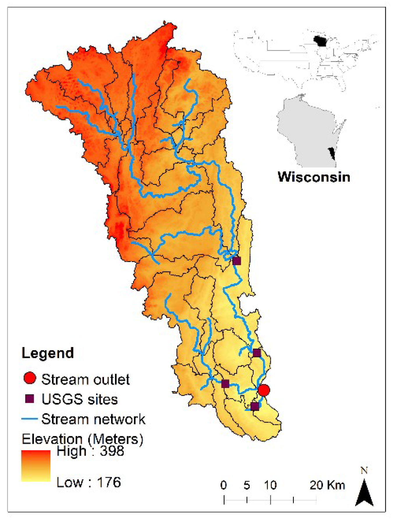
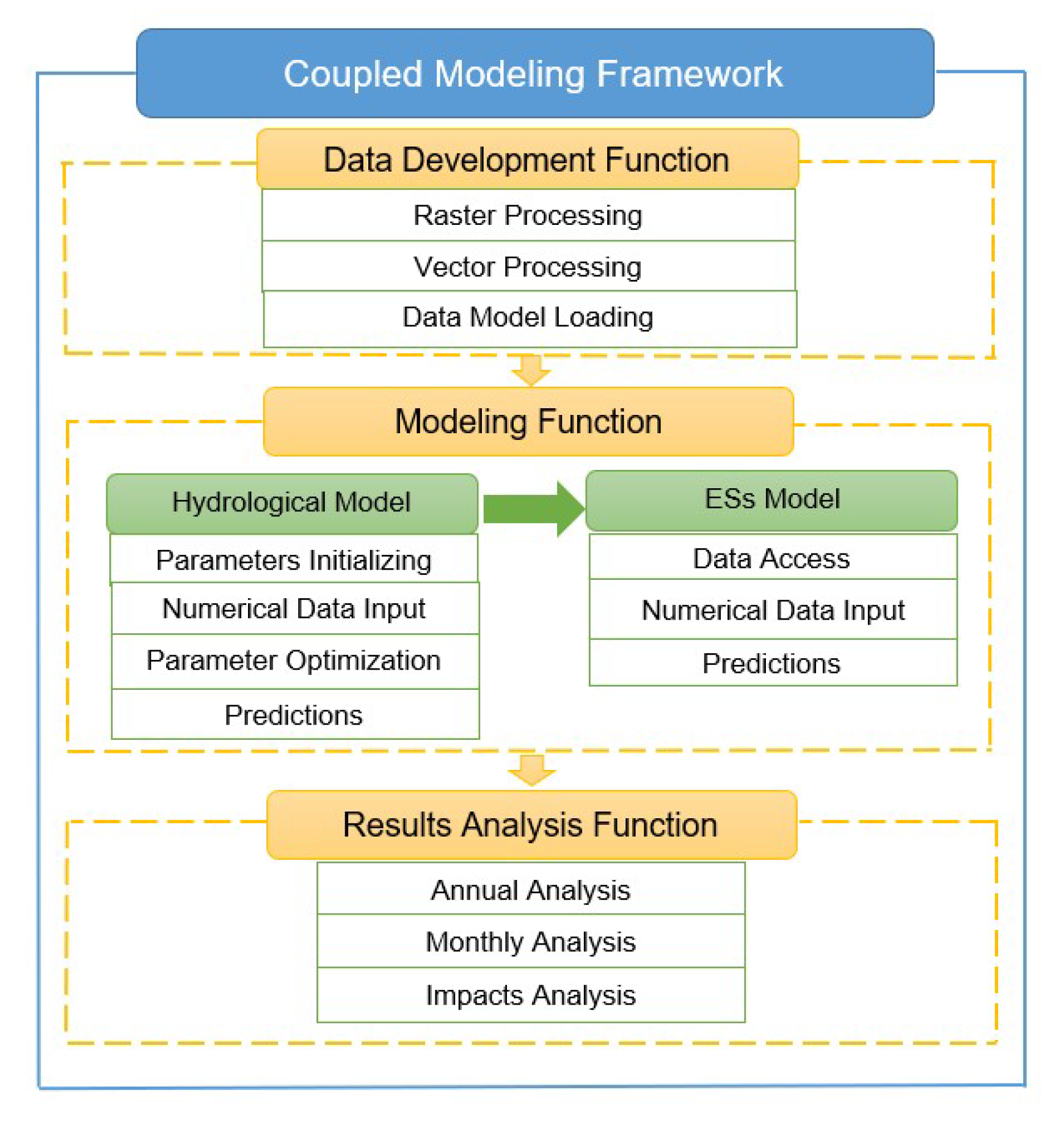
To overcome the weaknesses of previous impact studies of hydrologic ES as described above, a conceptual modeling framework [27] was applied in the Milwaukee River Basin to simulate three hydrologic ES indices under LULC and climate changes in this study. The framework includes a data-development function, a modeling function with hydrologic and ES models, and a results-analysis function. This framework can capture the fine temporal changes in some hydrologic ES (e.g., water provision, floods) and thus benefit relevant management plans and policies accordingly.
Based on above-mentioned challenges, two research questions are addressed:
  • How does LULC change impact hydrologic ES compared to climate change?
  • What are the changes of the hydrologic ES results at both annual and monthly scales?
Detailed methods, results, and discussions are covered in the following sections. In Section 2, the study area and scenarios design together with the framework are introduced. Results are presented in Section 3 and the discussion of each hydrologic and ES variable in different scenarios is provided in Section 4. Finally, conclusions are given in Section 5.

2. Materials and Methods

2.1. Study Site

The Milwaukee River basin (Figure 1) was selected as the study area. The Milwaukee metropolitan area in the southeast region of the basin contains 90 percent of the population and is highly urbanized. The LULC of the northern part is primarily agricultural. The topography of the basin consists of rolling moraine over bedrock [33]. The basin slopes downward from northwest (inland) to southeast (lakeshore). Three major rivers exist in the basin, namely Milwaukee, Menomonee, and Kinnickinnic. They merge in downtown Milwaukee and empty into Lake Michigan.
The climate type of the study area is humid continental climate (Köppen climate classification Dfa), which includes four distinct seasons with wide variations in temperature and precipitation. The mean temperature ranges from January was −7.3 °C to July 21.8 °C during 1971–2000 [34]. Average annual precipitation was about 862 mm, with wet summers and dry winters [35]. Mean annual streamflow measured at the main gauge (USGS 04087000) is approximately 219 mm during 1915–2008, with high in spring and low in late summer/early autumn [34].

2.2. Impact Scenarios

2.2.1. Scenarios Design

The same four scenarios (baseline, LULC change, climate change, and combined change) as in [34] were used (Table 1). For the baseline scenario, both LULC and climate forcing data come from the historical periods (National Land Cover Database (NLCD) 2001 and 1961–2000 climate data). For the LULC-change scenario, the LULC information was updated according to the 2050 LULC map (cellular automata (CA) 2050), and the climate data is the same as the baseline scenario. For the climate-change scenario, future climate data (downscaled 2046–2065) was used as input, and the LULC data is the same as the baseline scenario. For the combined-change scenario, both the LULC map and climate data were updated to a future period.
With the four scenarios, (1) the baseline scenario was used to evaluate historical ES; (2) the LULC-change impacts were evaluated by comparing the baseline scenario with the LULC-change scenario to show how LULC change impairs the future ecosystem services; (3) the climate-change impacts were evaluated by comparing the baseline and climate-change scenarios to reveal the projected effects on the studied hydrologic ES; (4) the combined scenario showed joint effects.

2.2.2. LULC Scenario

The NLCD 2001 with a resolution of 30 m × 30 m derived from satellite imageries from the Multi-Resolution Land Characteristics Consortium [36] was used as the baseline LULC map. It was clipped for the study area, and the LULC classes have been aggregated for simplicity, as shown in Figure 2a. The future LULC map (referred to as CA 2050 hereafter) was developed with two CA models for modeling residential and commercial expansion respectively [37]. The probability of a cell being converted to urban class (Ui) with the CA models is described as follows:
Ui = f (Pi, Ni, Ci, Ri),
where Pi is the global probability of conversion to urban LULC based on spatial-environmental and socio-economic influence, Ni is the neighborhood effect, Ci is the constraint factor for some areas that should be excluded (e.g., water, mountain), and Ri represents the random factor. Residential and commercial LULC information in 1990, 2000 and 2010 was employed for the CA model building, calibration and validation respectively, and a kappa index value (95.13%) was acquired in the assessment of the modeling performance.
LULC information and maps are presented in Table 2 and Figure 2. As shown in Table 2, the Developed class was projected to increase by 8.25% by 2050 whereas Planted/Cultivated, the other major LULC class was projected to decrease by 4.06%. The forest, shrubland, and other vegetation classes also were projected to decrease in different percentages. The two major LULC classes—Developed and Planted/Cultivated—with the most absolute changes in CA 2050 are depicted in Figure 2b. It can be clearly observed that expansion is projected around the current urban area, especially in the northern part of the study area where Planted/Cultivated class occupies the most.

2.2.3. Climate Scenario

The climate data in this study were derived from the dataset created by the Wisconsin Initiative on Climate Change Impacts [38]. The dataset is a result of statistical downscaling of several global climate models (GCMs), and we chose the one derived from the Canadian Center for Climate Modelling and Analysis’ Third Generation Coupled Global Climate Model (Acronym: cccma_cgcm3_1). This dataset has an approximately 10-km grid resolution and includes two periods: Historical (1961–2000) and future (2046–2065). The A1B greenhouse gas emissions scenario was selected as its CO2 concentration increase lies in the middle of the six Special Report on Emissions Scenarios (A1B, A1FI, A1T, A2, B1, and B2) [39].
Detailed climate data are presented in Table 3 and Figure 3. The data of selected GCM are very similar to the measured historical data (Table 3). The historical data has a slightly higher temperature (7.95 °C to 7.8 °C) and a similar standard deviation (0.8 °C and 0.9 °C). The precipitation data of historical and cccma_cgcm3_1 also are very closed (816mm and 814mm) and the standard deviation is a bit off (114mm and 146mm). The future climate data were projected to increase in temperature by 3.6 °C and an increase in precipitation by 54mm. Figure 3 depicts the average monthly changes in precipitation and temperature. Compared to baseline, the future climate scenario was projected to increase in precipitation for spring and winter while decreased in summer. The temperature generally was projected to increase with different amounts except for August.

2.3. Conceptual Modeling Framework

2.3.1. The Framework Workflow

The workflow of the conceptual framework created by Pan and Choi [27] is portrayed in Figure 4. The framework consists of three functions: Data development, modeling, and results analysis. The data-development function generates input data for hydrologic modeling and ES modeling with spatial and temporal processing of preliminary raster and vector data. The modeling function which includes both hydrologic and ES modeling, first conducts hydrologic modeling with calibration, validation, and projection, and then transports the hydrologic results to ES modeling to simulate hydrologic ES with ES parameters. The results-analysis function processes the hydrologic and ES results at different temporal scales in different scenarios.

2.3.2. Hydrologic Model

The Hydrologic Simulation Program-Fortran (HSPF) [40] was applied in this study to simulate streamflow. It is a comprehensive, physically based, semi-distributed hydrologic model that has been applied to study hydrologic variables in different impact scenarios in several previous studies [41,42,43,44,45].
The whole basin was first divided into subbasins based on stream network and then each subbasin was separated into three basic components, namely pervious land segments (PERLND), impervious land segments (IMPLND) and stream channel/reservoir (RCHRES) based on subbasin delineation, LULC classes, weather stations, and the ratio of perviousness and imperviousness for each LULC class [46].
The hydrologic processes of the model are based on the water-balance equation (Equation (2)).
S M C t = S M C t 1 + t = 1 T ( P t R t E T t G t ) ,
where SMC is the soil moisture content, t is time in days, T is the total days, P is the daily amounts of precipitation, R is the runoff, ET is the actual evapotranspiration, and G is the deep groundwater (percolation). All of the units are in mm.
Data products used in HSPF for this study are listed in Table 4.
The model parameters were calibrated and validated against the measured streamflow data in the previous study [34]. The comparison with the measured streamflow was conducted in terms of relative error (RE) and the Nash-Sutcliffe Efficiency (NSE). Sediment measurements have very limited availability, thus available daily measurements were averaged to monthly ones for comparison with simulations.

2.3.3. ES Model and Methods

Three modified quantitative methods [50] were employed with the capability of modeling at fine temporal scales. The input data for both hydrologic and ES modeling are at daily scale and the results are presented as daily and monthly, respectively.
● Water provision ES
The water provision ES was calculated as the index of water provisioning (WPI) (Equation (3)).
  WPI t =   MF t / MF EF MF t / MF EF + qne t / n t
where WPI is water provision index, MF is the mean flow (m3/s), MFEF is the long-term environmental flow requirement (m3/s), qne is the number of times the flow is less than environmental flow requirements in the time step, and n is the total number of units in the time step.
The WPI ranges from 0 to 1 where 0 indicates that provision of water quantity is not met at all, and 1 indicates that provision of water quantity is met for the entire time frame. Base on Tennant [51], 30% of the average flow for each month was used as MFEF to sustain good aquatic ecosystem functioning. The qne value was calculated on a daily basis.
● Flood regulation ES
The flood regulation ES was calculated as the flood regulation index (FRI) which incorporates three flood characteristics: Quantity, duration, and frequency of the flooding [52] as in Equation (4).
FRI = 1 exp [ w 1 · ( DF / DF LT ) + w 2 · ( QF / QF LT ) + w 3 · ( FE / FE LT ) ,
where DF is the duration of flood events (days), QF is the average magnitude of flooding events (m3/s), FE is the number of flood events per month or year, w1, w2, and w3 are user designed weights for each component of flooding (the sum of the weights is 1), and the LT subscript represents long-term (historical) data.
The FRI ranges from 0 to 1 with 0 representing maximum regulation needed and 1 representing no regulation needed. With this adopted method, the FRI will be calculated for each month with daily data to highlight seasonal changes in flood events and their effects. Long-term observed streamflow data from the study area were used to determine the flood flow (calculated as the 90th percentile of the flow), which then was used to calculate the long-term values for the average duration of flood events, the average magnitude of flood events, and the average number of flood events per year.
● Sediment retention ES
The sediment retention ES was calculated as the sediment regulation index (SRI), which is defined in Equation (5):
S R I = exp ( 1 ( S S m a x ) ) ,
where S is the monthly or annual erosion rate (T/ha) and Smax is the monthly or annual maximum allowable (or natural) rate of sediment (T/ha).
The range of the SRI is 0 to constant e. When the S equals to or is less than Smax, the SRI equals to or is greater than 1, meaning no regulation is needed. If the S is greater than Smax, the SRI is less than 1, indicating that sediment regulation is needed. The SRI is close to 0 when S is much larger than Smax. The Smax was determined to be 1.34 T/ha/year as the area-weighted US Department of Agriculture ‘T’ factor for tolerable soil loss [53]. It then was converted to monthly data, weighted by flow data.

3. Results

3.1. Hydrologic Modeling Under Impacts

An RE of 2.13% and an NSE of 0.71 were acquired by comparing simulated streamflow to observed data at the USGS site (04087000) for calibration. For the validation period, they are 4.87% and 0.54, respectively. The calibration and validation results of streamflow overall show good performance of the HSPF model. The simulated and observed sediment were compared at monthly and annual scales without calibration, since daily measurements were not available. The REs are 3.26% and 9.57%, respectively, which indicates overestimation at both scales.
The streamflow results simulated by HSPF in different scenarios are presented in Figure 5 and Table 5. According to Table 5 with averaged results of the entire simulation periods, streamflow decreases in the LULC scenario, increases in the climate scenario, and decreases in the combined scenario. In addition, according to Figure 3 and Figure 5a, the streamflow changes are primarily affected by precipitation changes as they show the same changing patterns in most months except August and November while temperature played a very insignificant role through the year. For instance, from December to May, the temperature increased which could lead to increased evaporation and decreased streamflow, however, streamflow increased with the increased precipitation instead. The combined scenario results are mostly the sum of the LULC and climate scenarios results except July and October. More detailed results can be found in Choi et al. [34].
The sediment results simulated by HSPF in different scenarios are shown in Figure 5b and Table 5. The annual average results of simulated sediment follow the pattern of streamflow as streamflow volume is the most important factor for sediment yield. As depicted in Figure 5b, the changes in monthly sediment results show a different pattern from streamflow, especially in March (opposite) and August (no change in the climate and combined scenarios). Also, the sediment in the combined scenario not simply equals to the sum up of the results of the LULC and climate scenarios. These differences in monthly patterns between streamflow and sediment are possibly due to other factors that are related to sediment yield, such as soil, topography, and vegetation cover.

3.2. Ecosystem Services Modeling Under Impacts

The modeling results of the three ES indices in the four scenarios were summarized and analyzed at different temporal scales.
The annual average results of the three ES indices in the four scenarios are presented in Table 6. The three ES indices increase slightly in the LULC scenario compared to those in the baseline scenario, which means the changes in the LULC scenario have positive effects on the results. The changes in the climate scenario decrease the WPI and the SRI but increase the FRI slightly. The changes in the combined scenario result in the decrease in the WPI and the slight increases in the FRI and the SRI. In sum, these results indicate that the effects of the three future scenarios on the annual ES results are so small that they are almost negligible.
The monthly ES results were converted to monthly average to examine the seasonal variability in the four scenarios. According to Figure 6, LULC change generally has slightly negative effects on the three indices whereas the climate and combined scenarios have large-negative impacts on some months and small-positive impacts on some other months. For the WPI in Figure 6a,d, changes in the climate and combined scenarios lead to the decreases from October to April (cold and dry seasons) and the increases from May to September, except for August (warm and humid seasons). For the FRI in Figure 6b,e, most of the increases happened from July to October (warm and humid) and most of the decreases happened in November, December, February and April (cold and dry). The decreases in the SRI (Figure 6c,f) exist in February, August, September, November, and December, and the increases exist in March, May, June. The changes in the monthly WPI, FRI, and SRI range from 0.004 to 0.15, 0.004 to 0.19, and 0.00016 to 0.16, respectively, which include some nonnegligible values compared to the annual average results. Furthermore, the climate and combined scenarios also affect the seasonal patterns of all the three indices. For instance, the WPI in the baseline and LULC scenarios increase from Jan to Feb while that in the climate and combined scenarios decrease. Similar examples can also be found in the FRI and the SRI results. The climate scenario leads to much larger changes in all the three indices than the LULC scenario at the monthly scale.
The monthly ES results in the four scenarios were further analyzed using boxplots in Figure 7. Figure 7a shows that compared to the baseline scenario, the climate and combined scenarios generate larger inter-month variations of the WPI than the LULC scenario while the medians of the four scenarios are similar. Comparing to the baseline scenario, the climate and combined scenarios also result in larger inter-month variations in the FRI than the LULC scenario whereas the medians are very close (Figure 7b). Figure 7c depicts the smaller inter-month variations and medians of the SRI in the climate and combined scenarios than those in the LULC and baseline scenarios.

4. Discussion

Based on Choi et al. [
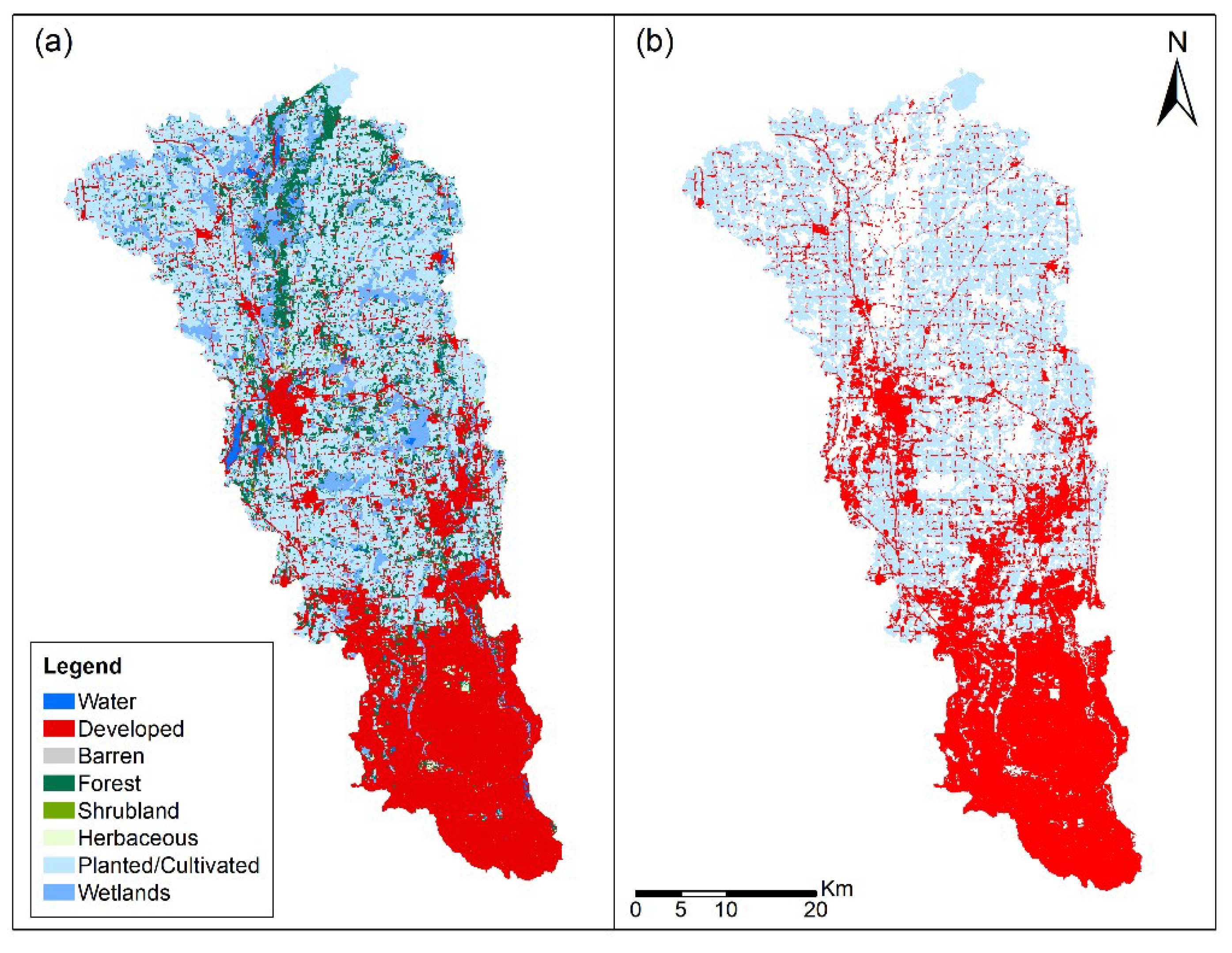
34], the impacts of LULC change on hydrologic simulations are negligible, due to the moderate LULC change and the offsetting effects among different LULC classes. Since only one future LULC scenario was considered in this study and the future LULC map (CA 2050) developed for this study is close to realistic urban development without any assumption of management plans, the impacts of the LULC change on the hydrologic variables and ES are very limited. Moreover, the impacts caused by urban expansion (increased by 60 km2) may also be offset by the reduction of planted/cultivated class, as shown in Table 2 (decreases by 40 km2). Such hydrologic simulation results lead to negligible hydrologic ES results. Gao et al. [54] reported that hydrologic ES decreased by 3.8% in water yield and increased by 16.3% in soil exports under agricultural expansion scenario while increased by 4.2% in water yield and decreased by 16.3% in soil exports under soil conservation scenarios. Hoyer and Chang [7] found out water yield is not sensitive to urban expansion scenarios as no difference found between results in different LULC-change scenarios while nutrient loading and sediment export are very sensitive to urban-expansion scenarios as changes ranged from –17% to 44% in sediment retention. Bai et al. [55] also stated that agricultural expansion resulted in the lowest water yield and the highest one was generated by forestry expansion. According to Logsdon and Chaubey [49], the extreme urban scenario had very limited impacts on hydrologic ES compared to the extreme agricultural scenario.
Climate change, unlike LULC change, has quite large impacts on hydrologic simulations [31] and ES. Fan et al. [29] found the climate scenario results in much more water yield than LULC scenario as future climate scenario created consistently increased water yield while LULC increased and then decreased water yield. Hoyer and Chang [7] stated that water yield is very sensitive to different climate-change scenarios compared to LULC scenarios (climate change results –6% to 15% water yield while no changes find among LULC scenarios). Samal et al. [
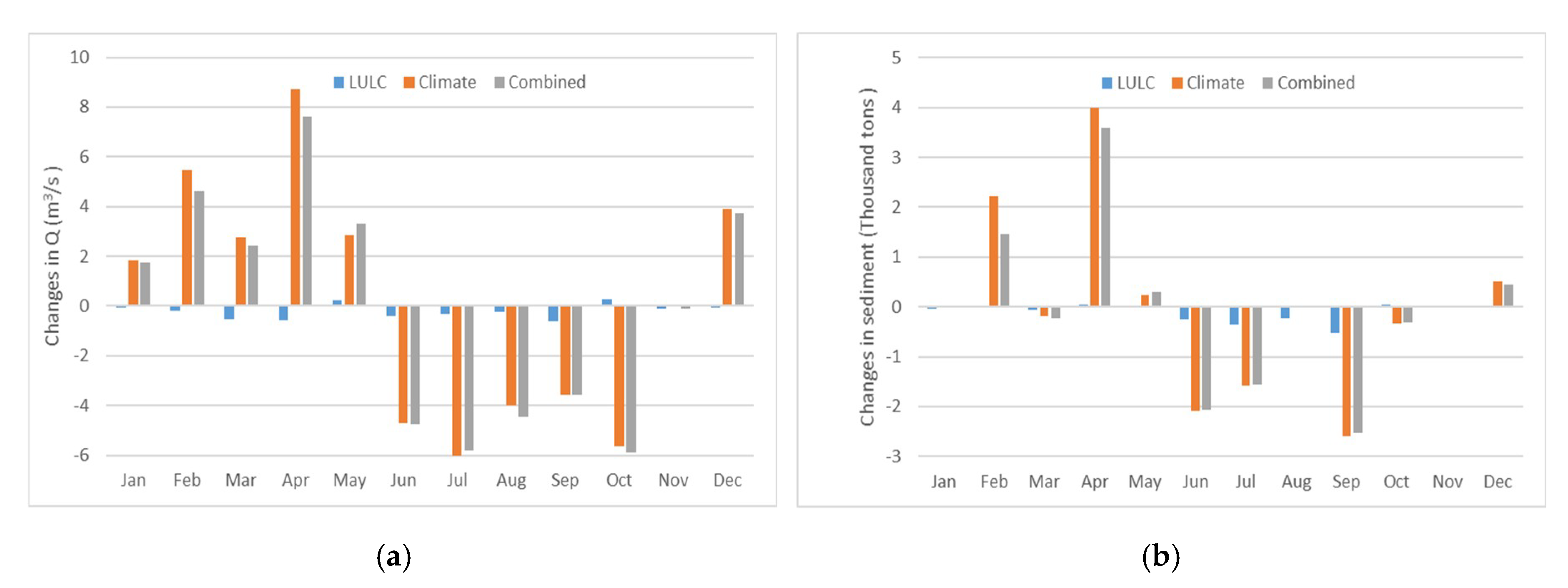
30] demonstrated that climate change has a greater influence on future aquatic ES than changes in LULC. Results from this study also indicated that the climate-change impacts on hydrologic ES are much larger than the LULC-change impacts. The impacts under climate change at monthly scale show that streamflow, sediment, WPI, FRI, and SRI have the changes from −6 to 9 m3/s, −2.5 to 4 thousand tons, −0.16 to 0.07, −0.19 to 0.1, and −0.58 to 0.15, compared to those under LULC-change impacts with the changes from −0.4 to 0.2 m3/s, −0.5 to 0.001 thousand tons, −0.02 to −0.001, −0.025 to 0.01, and −0.03 to 0, respectively.
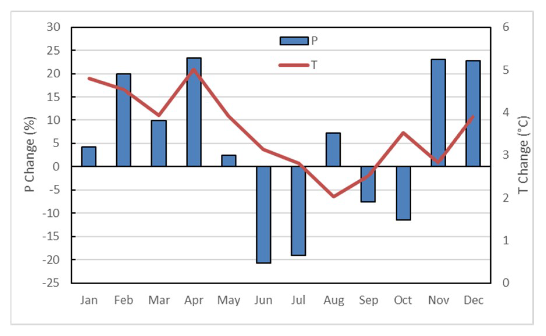
In term of climate-change impacts on streamflow, the annual precipitation increased about 6.6%, while the annual streamflow only increased 0.47% which is because even though the precipitation is the main source of streamflow, there are other factors influence the streamflow, such as soil moisture capacity, ground water level, and LULC classes etc. and therefore the streamflow did not increase or decrease with similar percentages as the precipitation. According to Choi et al. [34], when the precipitation decreased or increased with large amounts in some other GCMs which surpassed the capacity of the landscape system, the increases or decreases in streamflow are substantial. Furthermore, compared to the limited changes in the climate scenario at annual scale (0.13 m3/s, 0.14 thousand tons, −0.02, 0.01, and −0.01), the results at monthly scale show the large increased inter-monthly variation (4.73 m3/s, 1.20 thousand tons, 0.07, 0.06, and 0.17) and the changes in each month (−6.02 to 8.70 m3/s, −2.59 to 4.00 thousand tons, −0.16 to 0.07, −0.19 to 0.10, and −0.58 to 0.16) for streamflow, sediment, WPI, FRI, and SRI, respectively.
The WPI and streamflow showed a different changing pattern in monthly results. Since the most important input that affects streamflow volume is precipitation, with the projected increase in precipitation of 54 mm (Table 3), the streamflow volume increased (
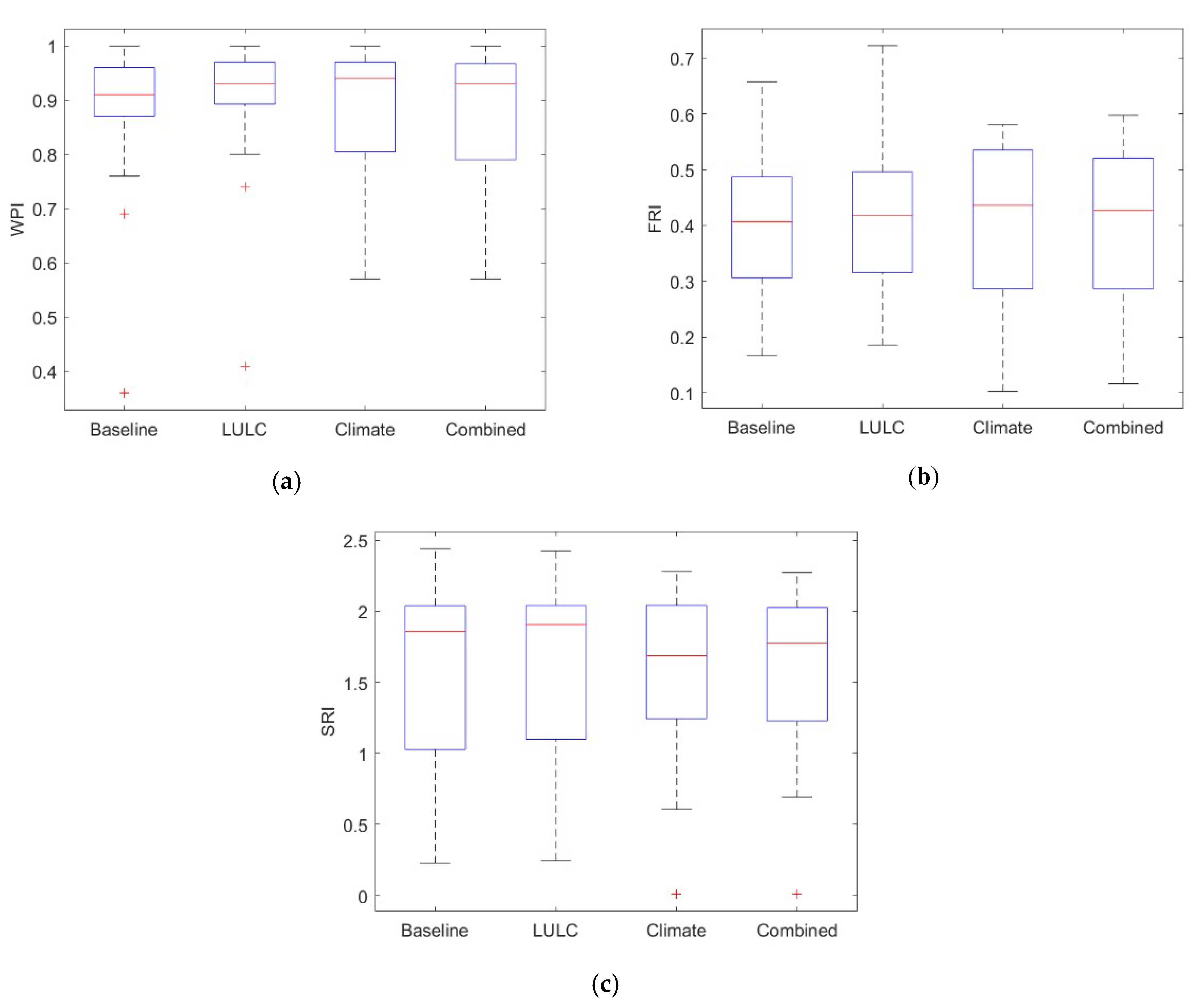
Table 5). However, as shown in Table 6 and 
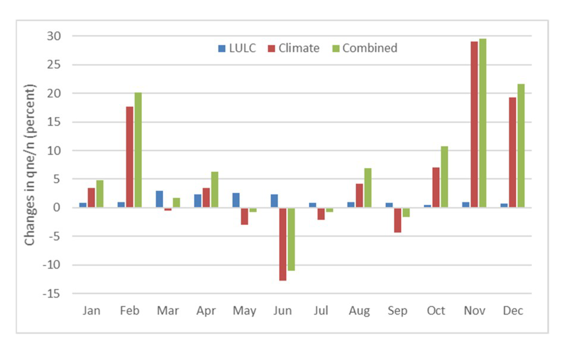
Figure 6d, the WPI in the climate scenario decreased. In the calculation method of WPI, the qne/n (Equation (3)), which is the monthly percentage that the water provision is not met the long-term requirement, were calculated and plotted (Figure 8). Compared Figure 8 to 
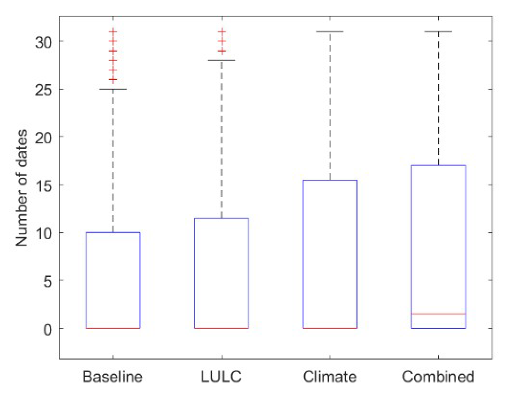
Figure 6d, it can be found out that the larger the monthly qne/n changes are, the larger the changes in the monthly WPI. Besides, as the results depicted in Figure 9, the climate scenario results in larger variation than the LULC and baseline scenarios. Such evidence demonstrates that the climate scenario actually results in more days that were not met long-term water provision requirement although streamflow volume in general increased, which leads to a decrease in the WPI. This finding demonstrates that compared to streamflow volume, decision-makers should pay more attention to the increased low flow events that could severely impact water provision.
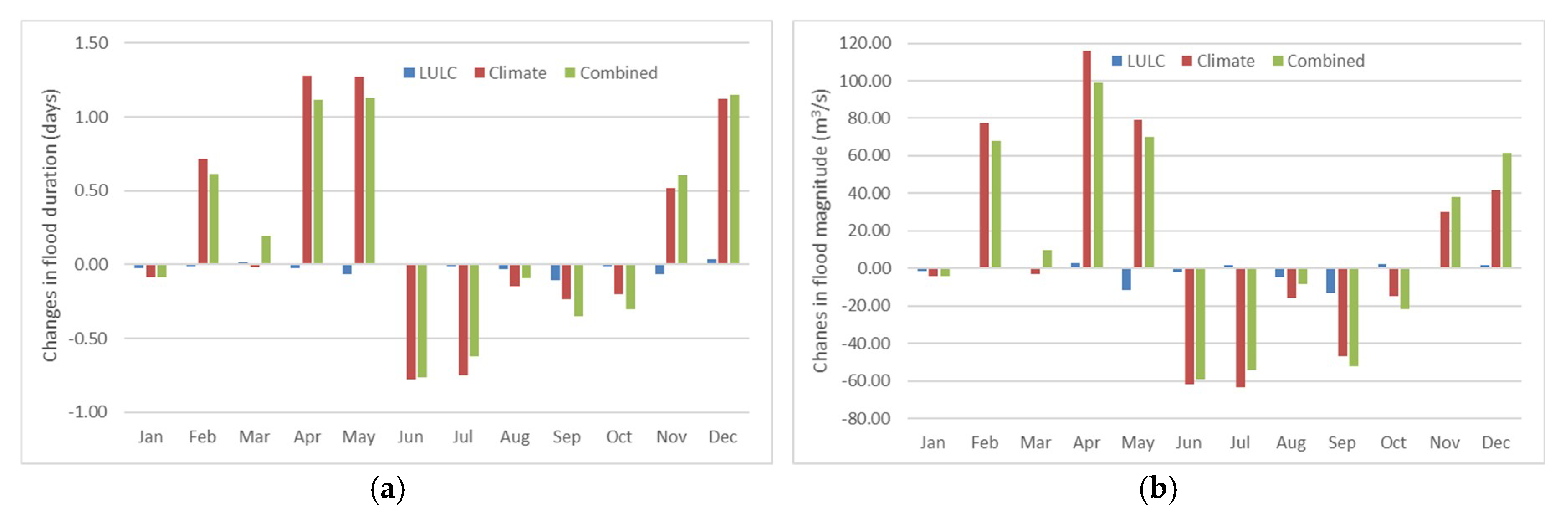
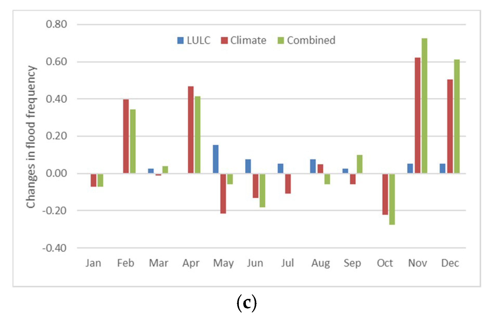
The FRI was found to be insensitive to any impact scenarios in annual results, however, it showed large changes in some months in the monthly analysis especially in the climate scenario. The three inputs of the FRI calculation (Equation (4)) were analyzed, and the results are presented in Figure 10 and Table 7. Based on Figure 10, the duration, magnitude, and frequency of flood in the climate scenario all increased significantly at February, April, May, November, and December when the precipitation is high and decreased significantly at June and July when the temperature is high. Such results correspond to the increases and decreases of the FRI in the climate scenario in different months, which demonstrates that even though the impacts are negligible at an annual scale, it can still be identified at a finer scale (e.g., monthly scale). Table 7 reveals that the LULC scenario reduced the duration and magnitude of the flood while the climate scenario increases all three of them. Flood frequency increased in all of the future scenarios compare to the baseline scenario. Findings from Table 7 could inform decision-makers that LULC change could mitigate climate-change impacts and they need to pay attention to the increased frequency of flood events.
The climate scenario results in large changes in the monthly SRI compared to annual results that are negligible. Comparing the changes in monthly averages of streamflow (Figure 5a) with that of the SRI (Figure 6f), it can be observed that not all the monthly results of the SRI followed the pattern of streamflow changes in the climate scenario, especially in April, May, July, August, and September, that the SRI has the same changing direction as the streamflow (more streamflow results in more sediment and then low SRI). Such findings indicate that the highest sediment regulation demand did not come with the largest precipitation, but it also was associated with temporal soil erodibility variation [56]. Such findings could remind decision-makers of the delay of sediment yield and soil erosion after the extreme events.

5. Conclusions

In this paper, with a conceptual modeling framework for hydrologic ES and the design of the scenario study, new insights were found regarding hydrologic ES under LULC and climate-change impacts in the urbanizing study area. Our study includes LULC and climate-change scenarios, and compares their impacts at both annual and monthly scales; and the latter are limited in hydrologic ES literature. The findings of this study could offer decision-makers and stakeholders more insights for land management plans.
The key findings of this study are that climate change has much larger impacts on hydrologic ES than LULC change, and also the results at the monthly scale show large increased inter-monthly variation and changes in each month compared to those at the annual scale. LULC-change impacts are small, due to the modest urban-expansion projection and the offsetting from the reduction of planted/cultivated LULC class. Streamflow, sediment, WPI, FRI, and SRI under climate-change impacts have the changes from −6 to 9 m3/s, −2.5 to 4 thousand tons, −0.16 to 0.07, −0.19 to 0.1, and −0.58 to 0.15, compared to those under LULC-change impacts with the changes from −0.4 to 0.2 m3/s, −0.5 to 0.001 thousand tons, −0.02 to −0.001, −0.025 to 0.01, and −0.03 to 0, respectively. In addition, compared to the limited changes of the results under climate change at annual scale (0.13 m3/s, 0.14 thousand tons, −0.02, 0.01, and −0.01), the results at monthly scale show the large increased inter-monthly variation (4.73 m3/s, 1.20 thousand tons, 0.07, 0.06, and 0.17) and changes in each month (−6.02 to 8.70 m3/s, −2.59 to 4.00 thousand tons, −0.16 to 0.07, −0.19 to 0.10, and −0.58 to 0.16). New insight was found that water provision does not correspond to streamflow volume, but is much sensitive to the low flow that does not meet the long-term requirement. Flood control is very sensitive to temporal scales with significant changes in monthly results but negligible changes in annual results, due to the sensitivity of the three input: Flood duration, flood magnitude and flood frequency. Sediment regulation results are more complicated, since they are not only affected by streamflow but seasonal erodibility, vegetation etc. In summary, climate change in this study has larger impacts on hydrologic ES than LULC change while LULC change could mitigate climate change with a reduction of plantation and cultivation. Such findings could provide decision-makers detailed and novel insights for management and conservation planning.
This study establishes a standard workflow for hydrologic ES modeling under LULC and climate-change impacts supported by national data products. Due to the timeframe limit and data availability, this study only utilized one LULC-change scenario and one climate model with one emission scenario. Such design has the limitation that the uncertainty from GCM projection cannot be eliminated, since comparison could not be made among the results of other GCMs, which could reduce the reliability of the results. Future studies could focus on adopting multiple LULC-change scenarios, other GCMs, and different emission scenarios for the analyses of tradeoffs and uncertainties. In addition, with more scenarios involved, the sensitivity of different temporal scales could also be further demonstrated. Finally, the modeling framework is still at the conceptual stage which includes all the necessary functions but not a user-friendly interface that could further assist stakeholders and the general public for understanding the processes and results. Such an interface could be built on a GIS platform, as a separate interface, or as a web-based interface depending on the workload and requirement from the stakeholders.

Author Contributions

Conceptualization, F.P.; methodology, F.P.; software, F.P.; validation, F.P. and W.C.; formal analysis, F.P. and W.C.; investigation, F.P. and W.C.; resources, F.P. and W.C.; data curation, F.P.; writing—original draft preparation, F.P.; writing—review and editing, F.P. and W.C.; supervision, W.C.

Funding

This research received no external funding.

Acknowledgments

The authors are grateful to the reviewers for their constructive comments and recommendation for this paper.

Conflicts of Interest

The authors declare no conflict of interest.

References

  1. Millennium Ecosystem Assessment. Ecosystems and Human Well-being: Biodiversity Synthesis; World Resources Institute: Washington, DC, USA, 2005. [Google Scholar]
  2. Guerry, A.D.; Polasky, S.; Lubchenco, J.; Chaplin-Kramer, R.; Daily, G.C.; Griffin, R.; Ruckelshaus, M.; Bateman, I.J.; Duraiappah, A.; Elmqvist, T.; et al. Natural capital and ecosystem services informing decisions: From promise to practice. Proc. Natl. Acad. Sci. USA 2015, 112, 7348–7355. [Google Scholar] [CrossRef] [PubMed] [Green Version]
  3. Daily, G.C.; Polasky, S.; Goldstein, J.; Kareiva, P.M.; Mooney, H.A.; Pejchar, L.; Ricketts, T.H.; Salzman, J.; Shallenberger, R. Ecosystem services in decision making: Time to deliver. Front. Ecol. Environ. 2009, 7, 21–28. [Google Scholar] [CrossRef]
  4. Bagstad, K.J.; Semmens, D.J.; Waage, S.; Winthrop, R. A comparative assessment of decision-support tools for Ecosystem services quantification and valuation. Ecosyst. Serv. 2013, 5, e27–e39. [Google Scholar] [CrossRef]
  5. Bagstad, K.J.; Semmens, D.J.; Winthrop, R. Comparing approaches to spatially explicit Ecosystem Service modeling: A case study from the San Pedro River, Arizona. Ecosyst. Serv. 2013, 5, 40–50. [Google Scholar] [CrossRef]
  6. Guswa, A.J.; Brauman, K.A.; Brown, C.; Hamel, P.; Keeler, B.L.; Sayre, S.S. Ecosystem Services: Challenges and opportunities for hydrologic modeling to support decision making. Water Resour. Res. 2014, 50, 4535–4544. [Google Scholar]
  7. Hoyer, R.; Chang, H. Assessment of freshwater Ecosystem Services in the Tualatin and Yamhill basins under climate change and urbanization. Appl. Geogr. 2014, 53, 402–416. [Google Scholar] [CrossRef]
  8. De Groot, R.; Alkemade, R.; Braat, L.; Hein, L.; Willemen, L. Challenges in integrating the concept of ecosystem services and values in landscape planning, management and decision making. Ecol. Complex. 2010, 7, 260–272. [Google Scholar] [CrossRef]
  9. Schröter, D.; Cramer, W.; Leemans, R.; Prentice, I.; Araújo, M.; Arnell, N.; Bondeau, A.; Bugmann, H.; Carter, T.; Gracia, C.; et al. Ecosystem Service Supply and Vulnerability to Global Change in Europe. Science 2005, 310, 1333–1337. [Google Scholar] [CrossRef]
  10. Lautenbach, S.; Seppelt, R.; Liebscher, J.; Dormann, C. Spatial and Temporal Trends of Global Pollination Benefit. PLoS ONE 2012, 7, e35954. [Google Scholar] [CrossRef]
  11. Eigenbrod, F.; Armsworth, P.; Anderson, B.; Heinemeyer, A.; Gillings, S.; Roy, D.; Thomas, C.; Gaston, K. Error propagation associated with benefits transfer-based mapping of Ecosystem Services. Biol. Conserv. 2010, 143, 2487–2493. [Google Scholar] [CrossRef]
  12. Parmesan, C.; Yohe, G. A globally coherent fingerprint of climate change impacts across natural systems. Nature 2003, 421, 37–42. [Google Scholar] [CrossRef]
  13. Wu, F.F.; Yang, X.H.; Shen, Z.Y. A three-stage hybrid model for regionalization, trends and sensitivity analyses of temperature anomalies in China from 1966 to 2015. Atmos. Res. 2018, 205, 80–92. [Google Scholar] [CrossRef]
  14. Yang, X.H.; Li, Y.Q.; Wang, K.W.; Sun, B.Y.; Ye, Y.; Li, M.S. Improved Gray-Encoded Evolution Algorithm Based on Chaos Cluster for Parameter Optimization of Moisture Movement. Therm. Sci. 2017, 21, 15–20. [Google Scholar] [CrossRef]
  15. Wang, K.; Yang, X.; Liu, X.; Liu, C. A simple analytical infiltration model for short-duration rainfall. J. Hydrol. 2017, 555, 141–154. [Google Scholar] [CrossRef]
  16. EEA. Climate Change, Impacts and Vulnerability in Europe 2012—An Indicator-Based Report; EEA Report No 12/2012; European Environment Agency: Copenhagen, Denmark, 2012. [Google Scholar]
  17. Staudinger, M.D.; Grimm, N.B.; Staudt, A.; Carter, S.L.; Stuart Iii, F.S.; Kareiva, P.; Ruckelshaus, M.; Stein, B.A. Impacts of Climate Change on Biodiversity, Ecosystems, and Ecosystem Services; Technical Input to the 2013 National Climate Assessment; U.S. Geological Survey: Washington, DC, USA, 2012.
  18. Boyd, J. 2010. Ecosystem services and climate adaptation. Issue brief. Available online: https://www.rff.org/publications/issue-briefs/ecosystem-services-and-climate-adaptation/ (accessed on 31 January 2018).
  19. Shaw, M.R.; Pendleton, L.; Cameron, D.R.; Morris, B.; Bachelet, D.; Klausmeyer, K.; MacKenzie, J.; Conklin, D.R.; Bratman, G.N.; Lenihan, J.; et al. The impact of climate change on California’s ecosystem services. Clim. Chang. 2011, 109, 465–484. [Google Scholar] [CrossRef] [Green Version]
  20. Polasky, S.; Nelson, E.; Pennington, D.; Johnson, K.A. The impact of landuse change on Ecosystem Services, biodiversity and returns to landowners: A case study in the state of Minnesota. Environ. Resour. Econ. 2011, 48, 219e242. [Google Scholar] [CrossRef]
  21. Liu, T.; Merrill, N.H.; Gold, A.J.; Kellogg, D.Q.; Uchida, E. Modeling the production of multiple Ecosystem Services from agricultural and forest landscapes in Rhode Island. Agric. Resour. Econ. Rev. 2013, 42, 251–274. [Google Scholar] [CrossRef]
  22. Portela, R.; Rademacher, I. A dynamic model of patterns of deforestation and their effect on the ability of the Brazilian Amazonia to provide Ecosystem Services. Ecol. Model. 2001, 143, 115–146. [Google Scholar] [CrossRef]
  23. Nelson, E.; Mendoza, G.; Regetz, J.; Polasky, S.; Tallis, H.; Cameron, D.; Chan, K.; Daily, G.; Goldstein, J.; Kareiva, P.; et al. Modeling multiple Ecosystem Services, biodiversity conservation, commodity production, and tradeoffs at landscape scales. Front. Ecol. Environ. 2009, 7, 4–11. [Google Scholar] [CrossRef]
  24. Chang, H.; Bonnette, M.R. Climate change and water-related ecosystem services: Impacts of drought in California, USA. Ecosyst. Health Sustain. 2016, 2, e01254. [Google Scholar] [CrossRef]
  25. Arkema, K.K.; Guannel, G.; Verutes, G.; Wood, S.A.; Guerry, A.; Ruckelshaus, M.; Kareiva, P.; Lacayo, M.; Silver, J.M. Coastal habitats shield people and property from sea-level rise and storms. Nat. Clim. Change 2013, 3, 913–918. [Google Scholar] [CrossRef]
  26. Roy, S.B.; Chen, L.; Girvetz, E.H.; Maurer, E.P.; Mills, W.B.; Grieb, T.M. Projecting water withdrawal and supply for future decades in the US under climate change scenarios. Environ. Sci. Technol. 2012, 46, 2545–5256. [Google Scholar] [CrossRef] [PubMed]
  27. Pan, F.; Choi, W. A Conceptual Modeling Framework for Hydrologic Ecosystem Services. Hydrology 2019, 6, 14. [Google Scholar] [CrossRef]
  28. Cline, J.; Lorenz, J.; Swain, E. Linking Hydrologic Modeling and Ecologic Modeling: An Application of Adaptive Ecosystem Management in the Everglades Mangrove Zone of Florida Bay. In Proceedings of the 2nd International Congress on Environmental Modelling and Software, Osnabruck, Germany, 14–17 June 2004. [Google Scholar]
  29. Wlotzka, M.; Heuveline, V.; Klatt, S.; Haas, E.; Kraus, D.; Butterbach-Bahl, K.; Kraft, P.; Breuer, L. Simulation of Land Management Effects on Soil N2O Emissions Using a Coupled Hydrology-Biogeochemistry Model on the Landscape Scale; Willi, F., M. Zuhair, N., Thomas, S., Eds.; Springer: Berlin/Heidelberg, Germany, 2014; pp. 1–22. [Google Scholar]
  30. Fan, M.; Shibata, H.; Wang, Q. Optimal conservation planning of multiple hydrological ecosystem services under land use and climate changes in Teshio river watershed, northernmost of Japan. Ecol. Indic. 2016, 62, 1–13. [Google Scholar] [CrossRef]
  31. Samal, N.R.; Wollheim, W.; Zuidema, S.; Stewart, R.; Zhou, Z.; Mineau, M.M.; Borsuk, M.; Gardner, K.H.; Glidden, S.; Huang, T.; et al. A coupled terrestrial and aquatic biogeophysical model of the Upper Merrimack River watershed, New Hampshire, to inform ecosystem services evaluation and management under climate and land-cover change. Ecol. Soc. 2017, 22, 18. [Google Scholar] [CrossRef]
  32. Sample, J.E.; Baber, I.; Badger, R. A spatially distributed risk screening tool to assess climate and land use change impacts on water-related ecosystem services. Environ. Model. Softw. 2016, 83, 12–26. [Google Scholar] [CrossRef]
  33. Wisconsin Department of Natural Resources. The State of the Milwaukee River Basin; Department of Natural Resources: Madison, WI, USA, 2001.
  34. Choi, W.; Pan, F.; Wu, C. Impacts of climate change and urban growth on the streamflow of the Milwaukee River (Wisconsin, USA). Reg. Environ. Chang. 2017, 17, 889–899. [Google Scholar] [CrossRef]
  35. Wisconsin State Climatology Office. Historical Climate Data. Available online: http://www.aos.wisc.edu/*sco/clim-history/division/4709- climo.html (accessed on 19 May 2015).
  36. Homer, C.H.; Fry, J.A.; Barnes, C.A. The National Land Cover Database U.S. Geol. Surv. Fact Sheet 2012, 4, 2012–3020. [Google Scholar]
  37. Li, W.; Wu, C.; Choi, W. Predicting future urban impervious surface distribution using cellular automata and regression analysis. Earth Sci. Inform. 2018, 11, 19–29. [Google Scholar] [CrossRef]
  38. Wisconsin Initiative on Climate Change Impacts. Wisconsin’s Changing Climate: Impacts and Adaptation, Nelson Institute for Environmental Studies, University of Wisconsin-Madison and the Wisconsin Department of Natural Resources. Available online: http://www.wicci.wisc.edu/report/2011_WICCI-Report.pdf (accessed on 17 August 2017).
  39. Meehl, G.A.; Stocker, T.F.; Collins, W.D.; Friedlingstein, P.; Gaye, A.T.; Gregory, J.M.; Kitoh, A.; Knutti, R.; Murphy, J.M.; Noda, A.; et al. Climate Change 2007: The Physical Science Basis; Cambridge University Press: Cambridge, MA, USA, 2007; pp. 747–845. [Google Scholar]
  40. Duda, P.B.; Hummel, P.R.; Donigian, A.S., Jr.; Iimhoff, J.C. BASINS/HSPF Model Use, Calibration and Validation. Trans. ASABE 2012, 55, 1523–1547. [Google Scholar] [CrossRef]
  41. Alarcon, V.J.; Mcanally, W.; Diaz-Ramirez, J.; Martin, J.; Cartwright, J. A Hydrological Model of the Mobile River Watershed, Southeastern USA. AIP Conf. Proc. 2009, 1148, 641–645. [Google Scholar]
  42. Hsu, S.M.; Chiou, L.B.; Lin, G.F.; Chao, C.H.; Wen, H.Y.; Ku, C.Y. Applications of simulation technique on debris-flow hazard zone delineation: A case study in Hualien county, Taiwan. Nat. Hazards Earth Syst. Sci. 2010, 10, 535–545. [Google Scholar] [CrossRef]
  43. Chen, J.; Theller, L.; Gitau, M.W.; Engel, B.A.; Harbor, J.M. Urbanization impacts on surface runoff of the contiguous United States. J. Environ. Manag. 2017, 187, 470–481. [Google Scholar] [CrossRef] [PubMed]
  44. Hayashi, S.; Murakami, S.; Xu, K.; Watanabe, M.; Xu, B. Daily runoff simulation by an integrated catchment model in the middle and lower regions of the Changjiang basin, China. J. Hydrol. Eng. 2008, 13, 846–862. [Google Scholar] [CrossRef]
  45. Tzoraki, O.; Nikolaidis, N.P. A generalized framework for modeling the hydrologic and biogeochemical response of a Mediterranean temporary river basin. J. Hydrol. 2007, 346, 112–121. [Google Scholar] [CrossRef]
  46. Bicknell, B.R.; National Exposure Research Laboratory (U.S.). Hydrological Simulation Program—FORTRAN User’s Manual for Version 11; Environmental Protection Agency: Research Triangle Park, NC, USA, 1997. [Google Scholar]
  47. U.S. Geological Survey. USGS National Elevation Dataset (NED) 1 Arc-Second Downloadable Data Collection from The National Map 3D Elevation Program (3DEP)—National Geospatial Data Asset (NGDA) National Elevation Data Set (NED): U.S. Geological Survey; U.S. Geological Survey: Reston, VA, USA, 2016.
  48. Vogelmann, J.E. Completion of the 1990s national land cover data set for the conterminous United States from Landsat thematic mapper data and ancillary data sources. Photogramm. Eng. Remote Sens. 2001, 67, 650–655. [Google Scholar]
  49. U.S. Geological Survey. National Water Information System Data Available on the World Wide Web (USGS Water Data for the Nation). Available online: http://waterdata.usgs.gov/nwis/ (accessed on 10 June 2012).
  50. Logsdon, R.A.; Chaubey, I. A quantitative approach to evaluating ecosystem services. Ecol. Model. 2013, 257, 57–65. [Google Scholar] [CrossRef]
  51. Tennant, D.L. Instream flow regimens for fish, wildlife, recreation and related environmental resources. Fisheries 1976, 1, 6–10. [Google Scholar] [CrossRef]
  52. De Guenni, L.B.; Cardoso, M.; Goldammer, J.; Hurtt, G.; Mata, L.J.; Ebi, K.; House, J.; Valdes, J. Regulation of natural hazards: Floods and fires. In Ecosystems and Human Well-Being: Current State and Trends; Norgaard, R., Ed.; Island Press: Washington, DC, USA, 2005. [Google Scholar]
  53. Soil Survey Staff, Natural Resources Conservation Service, United States Department of Agriculture. Web Soil Survey. Available online: http://websoilsurvey.nrcs.usda.gov/ (accessed on 25 September 2018).
  54. Gao, J.; Li, F.; Gao, H.; Zhou, C.; Zhang, X. The impact of land-use change on water-related ecosystem services: A study of the Guishui River Basin, Beijing, China. J. Clean. Prod. 2017, 163, 148–155. [Google Scholar] [CrossRef]
  55. Bai, Y.; Zheng, H.; Ouyang, Z.; Zhuang, C.; Jiang, B. Modeling hydrological ecosystem services and tradeoffs: A case study in Baiyangdian watershed, China. Environ. Earth Sci. 2013, 70, 709–718. [Google Scholar] [CrossRef]
  56. Bajracharya, R.M.; Lal, R. Seasonal Soil Loss and Erodibility Variation on a Miamian Silt Loam Soil. (Soil and Water Management and Conservation). Soil Sci. Soc. Am. J. 1992, 56, 1560. [Google Scholar] [CrossRef]
Figure 1. The Milwaukee River basin boundary and elevation, along with subbasins delineated for hydrologic modeling, US Geological Survey (USGS) streamflow measurement sites, and stream network.
Climate 07 00059 g001
Figure 2. LULC of 2001 (a) and Developed and Planted/Cultivated classes of 2050 (b) for the Milwaukee River basin.
Climate 07 00059 g002
Figure 3. Distribution of average monthly changes in temperature and precipitation between 1961–2000 and 2046–2065 by the GCM.
Climate 07 00059 g003
Figure 4. Workflow of the modeling framework [27].
Climate 07 00059 g004
Figure 5. Changes in monthly streamflow (a) and sediment (b) resulting from three future scenarios.
Climate 07 00059 g005
Figure 6. Monthly averages of ES in the four scenarios (a: WPI, b: FRI, c: SRI) and the changes between the three future scenarios and the baseline scenario (d: WPI, e: FRI, f: SRI).
Climate 07 00059 g006
Figure 7. Distribution of the monthly results of three ES indices in the four scenarios (a: WPI; b: FRI; c: SRI).
Climate 07 00059 g007
Figure 8. Monthly averages of changes in percentage that the long-term water provision requirement is not met.
Climate 07 00059 g008
Figure 9. Distribution of the number of days that long-term water provision requirement is not met in the four scenarios based on the monthly results.
Climate 07 00059 g009
Figure 10. Changes in monthly averages of inputs for the FRI calculation between baseline and three future scenarios (a. flood duration; b. flood magnitude; c. flood frequency).
Climate 07 00059 g010aClimate 07 00059 g010b
Table 1. Hydrologic and ecosystem services (ES) modeling setup consisting of different climate and land use/landcover (LULC) scenarios [34].
Modeling ScenariosAcronymClimate DataLULC Data
BaselineBaselineDownscaled 1961–2000NLCD 2001
LULC change onlyLULCDownscaled 1961–2000CA 2050
Climate change onlyClimateDownscaled 2046–2065NLCD 2001
LULC and climate combined changesCombinedDownscaled 2046–2065CA 2050
Table 2. LULC statistics and projected changes by 2050.
LULC ClassesCurrent (km2)Current (%)2050 (km2)2050 (%)Change (%)
Water21.210.9620.940.94−1.27
Developed714.2832.18773.1834.838.25
Barren1.830.081.850.081.09
Forest240.4710.83224.4810.11−6.65
Shrubland150.6814.020.63−6.53
Herbaceous15.870.71150.68−5.48
Planted/Cultivated949.5642.77911.0341.04−4.06
Wetlands261.7111.79259.4511.69−0.86
Table 3. Average annual temperature (°C) and precipitation (mm) for 1961–2000 and 2046–2065 from the historical data and downscaled global climate models (GCM). Standard deviations across the years are in parenthesis.
1961–20002046–2065
TemperaturePrecipitationTemperaturePrecipitation
Historical7.95 (0.8)816 (114)N/AN/A
cccma_cgcm3_17.8 (0.9)814 (146)11.4 (0.9)868 (151)
ChangeN/AN/A3.654
Table 4. Summary of datasets used for hydrologic modeling.
Data SetsSpatial ResolutionSource
Digital elevation data30 mUS Geological Survey (USGS) [47]
Land cover map30 m NLCD [48]
Climate data10 kmWisconsin Initiative on Climate Change Impacts [38]
Streamflow and sediments yield dataN/AUSGS [49]
Table 5. Summary of results for hydrologic modeling.
Modeling ScenariosStreamflow (m3/s)Sediment (Thousand Tons)
Baseline19.8720.40
LULC19.6419.04
Climate20.0020.54
Combined19.7819.56
Table 6. Summary of results for ES modeling.
Modeling ScenariosWPIFRISRI
Baseline0.890.391.57
LULC0.910.411.61
Climate0.870.401.56
Combined0.860.401.58
Table 7. Summary of inputs for the FRI calculation.
Modeling ScenariosFlood Duration (days)Flood Magnitude (m3/s)Flood Frequency
Baseline2.64201.717.46
LULC2.46187.057.97
Climate2.82203.078.68
Combined2.70198.129.05

