Toward a Regional-Scale Seasonal Climate Prediction System over Central Italy Based on Dynamical Downscaling


Abstract
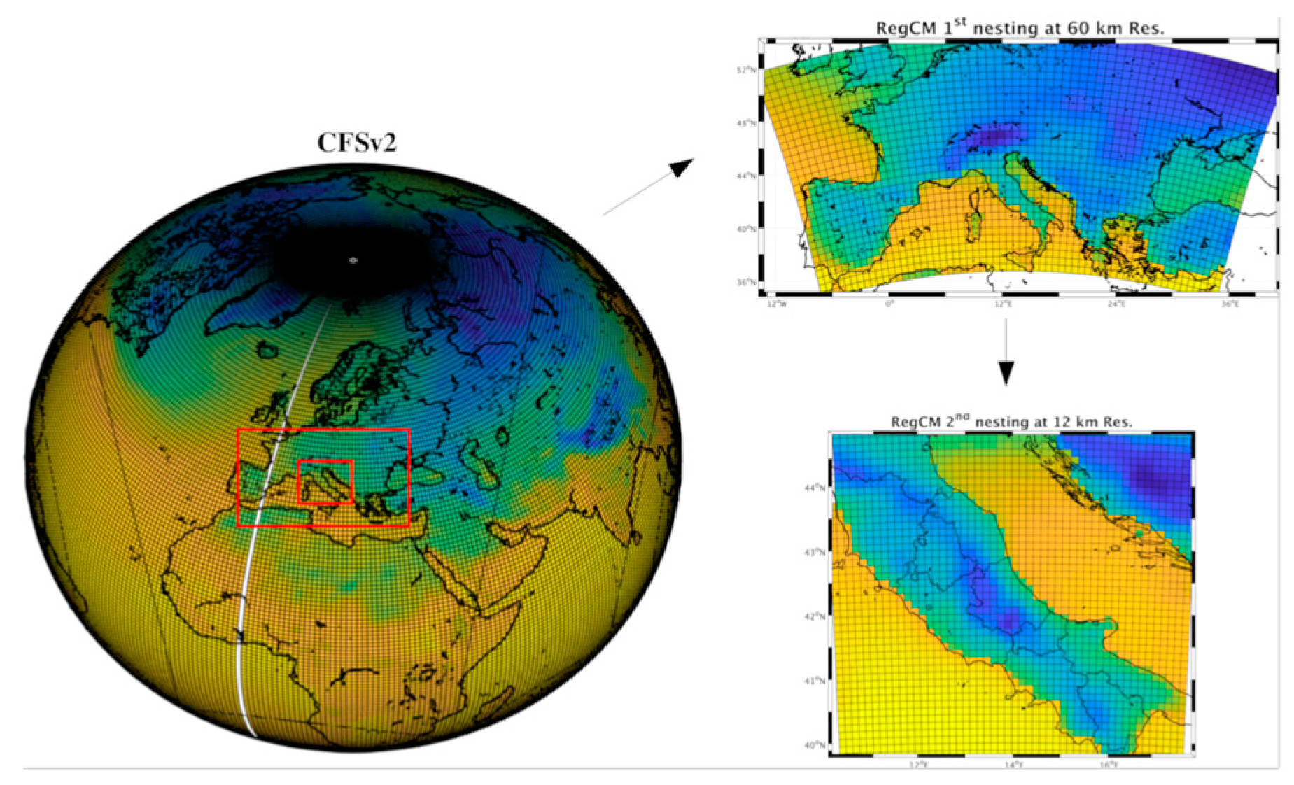
:1. Introduction
2. Modeling Chain and Evaluation Metrics
3. Results and Discussion
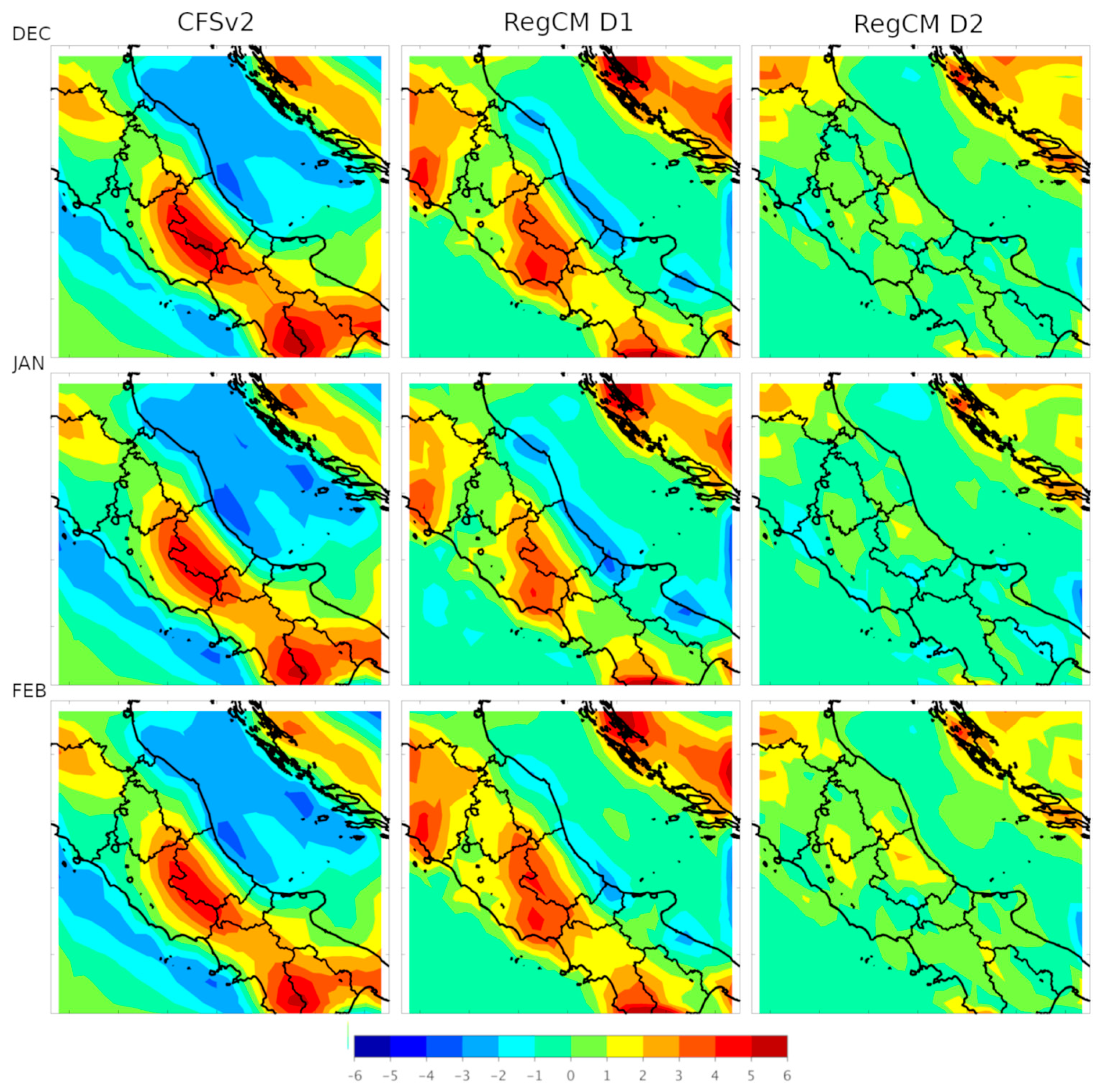
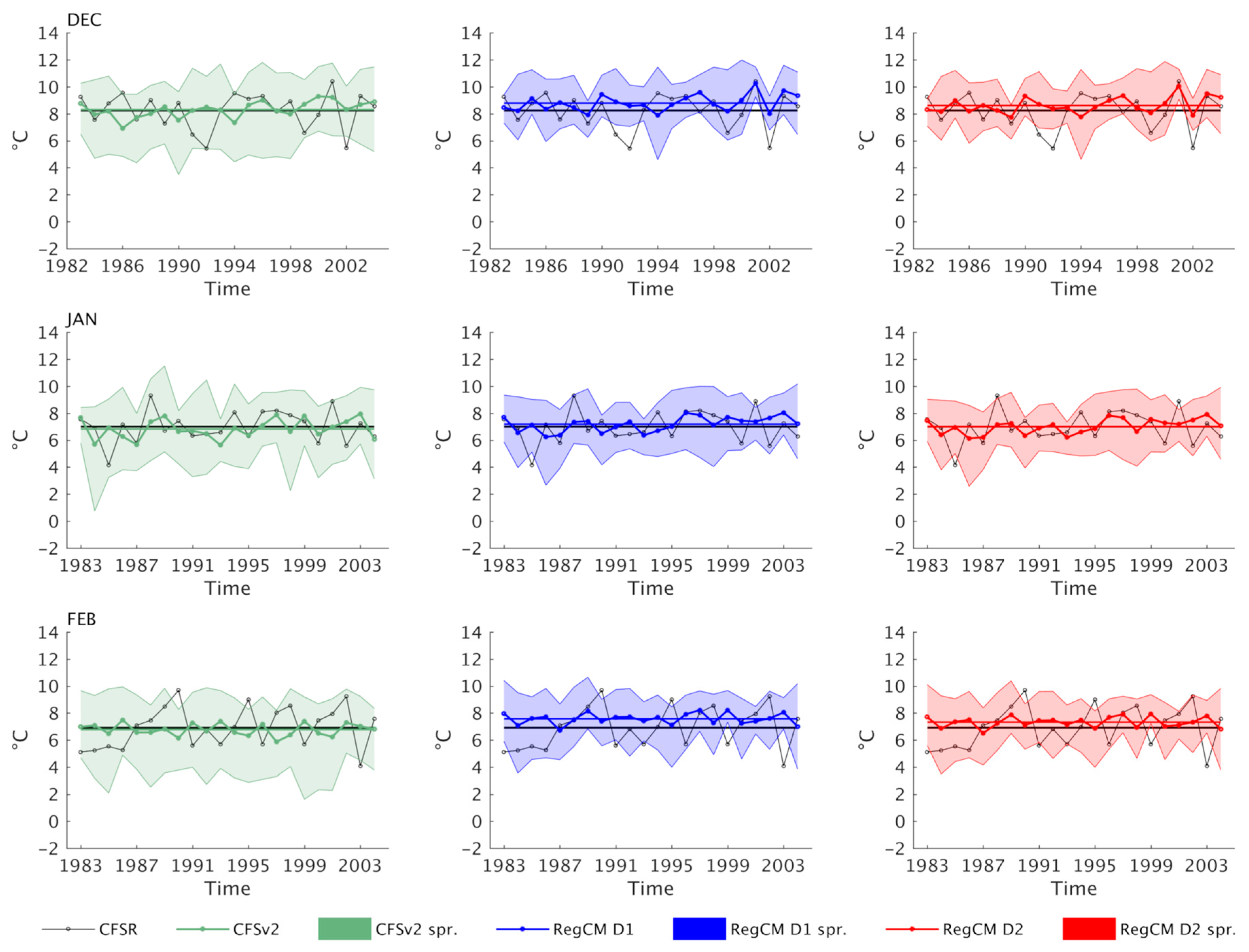
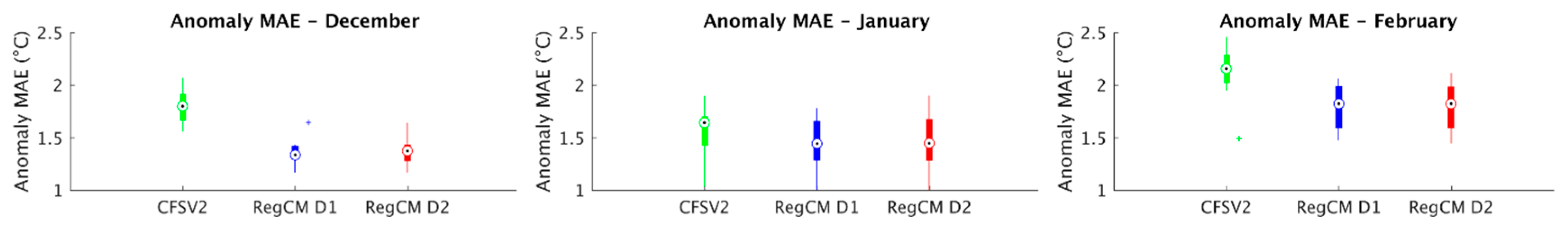
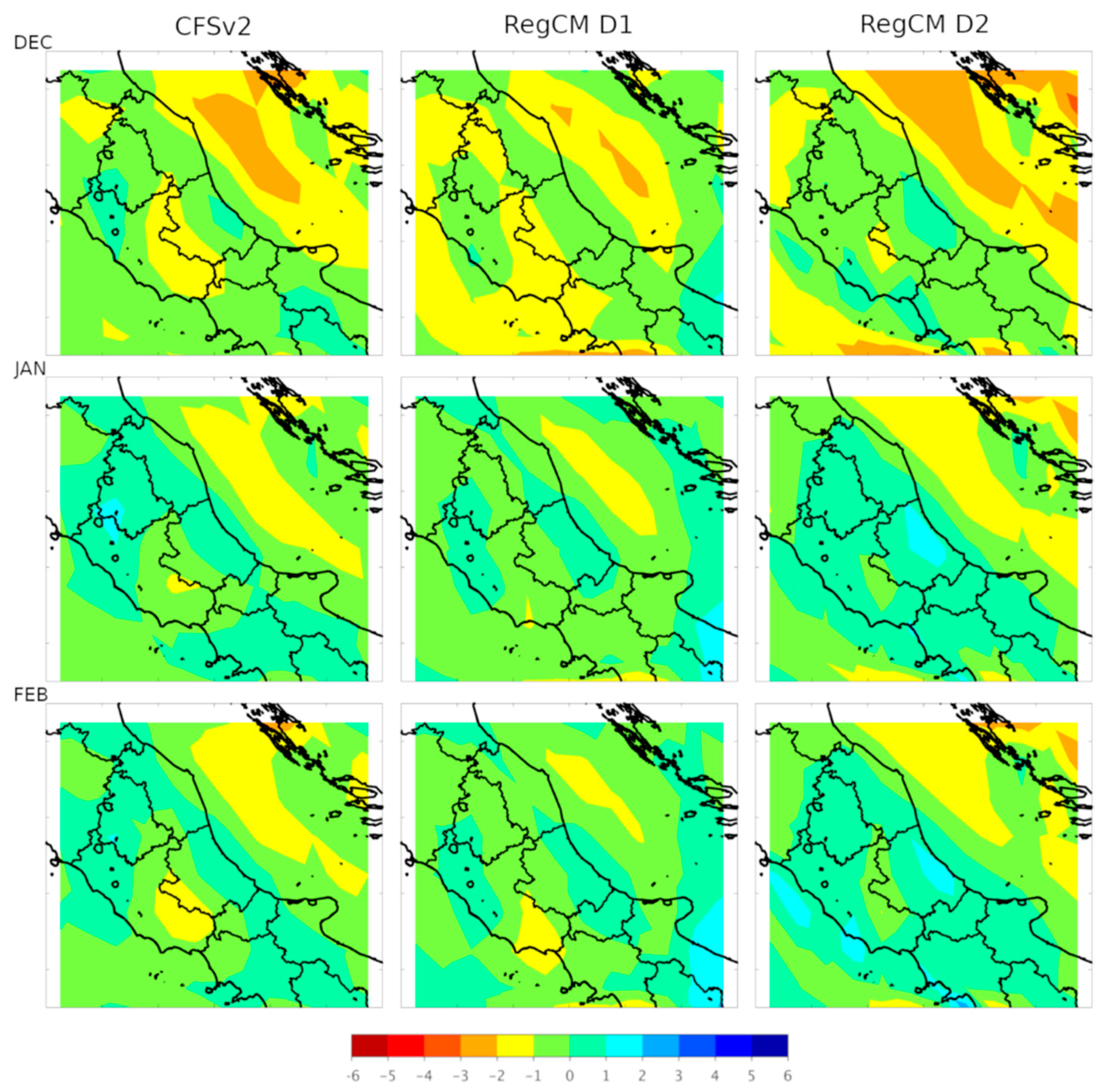
3.1. Temperature Assessment
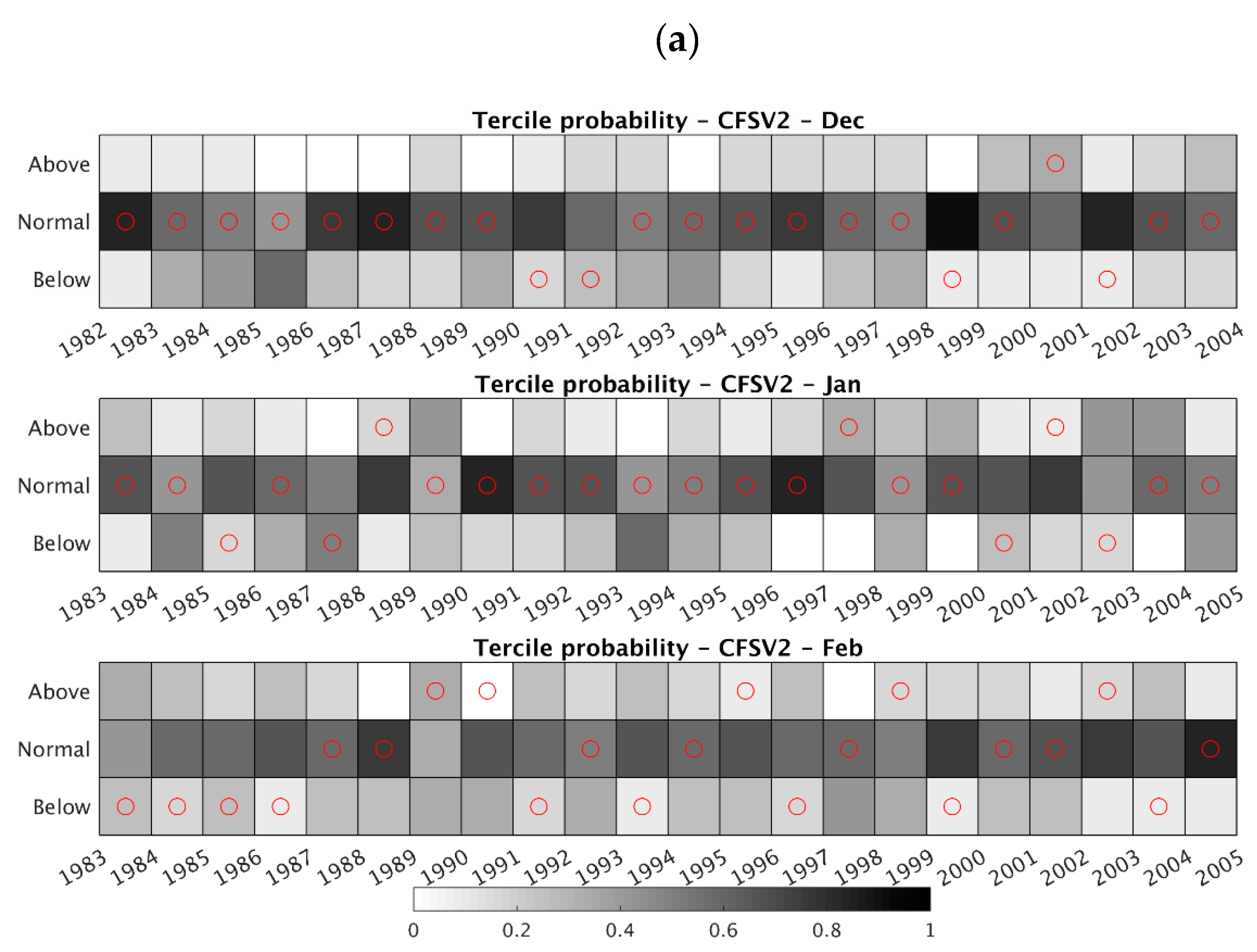
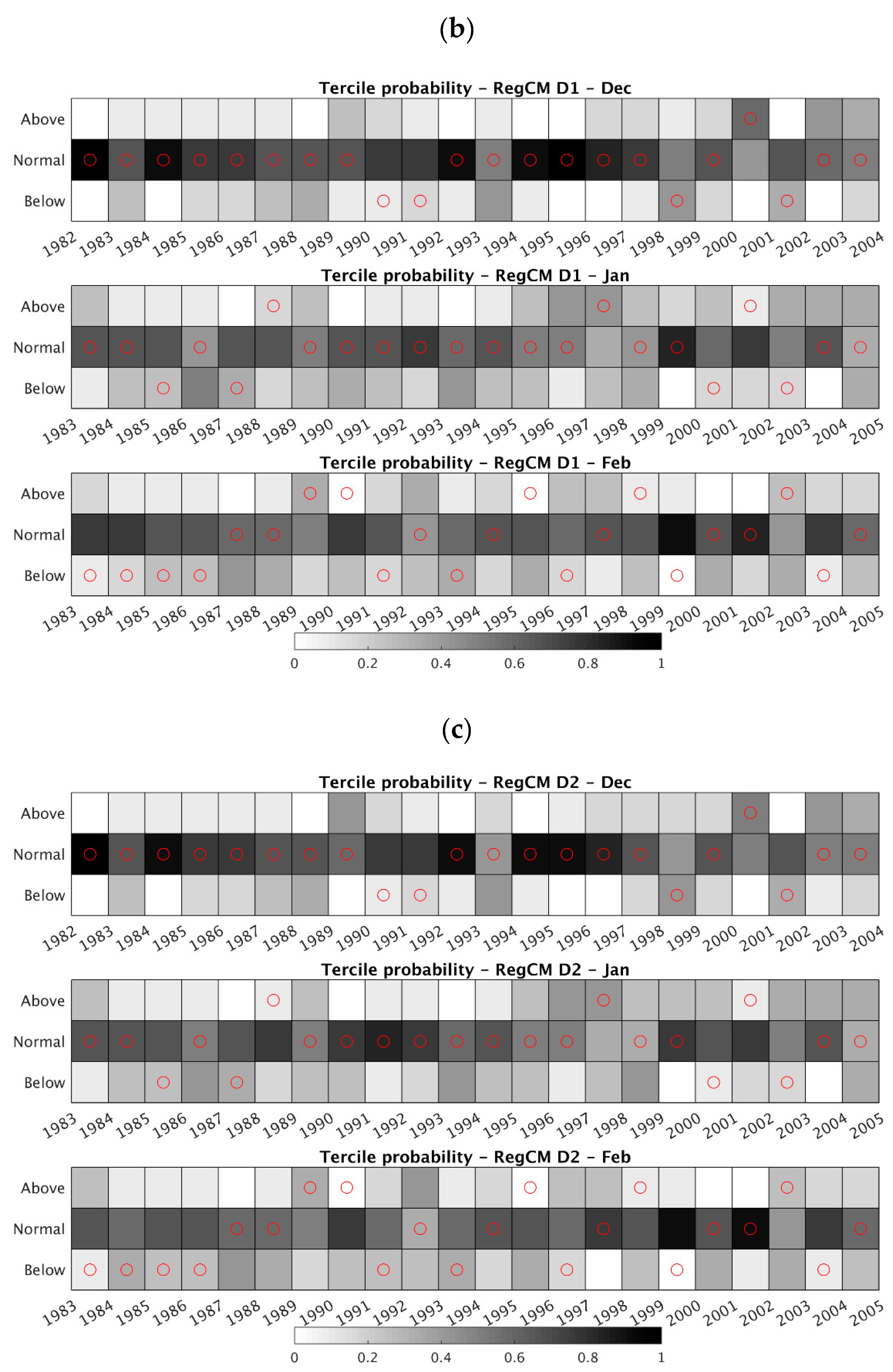
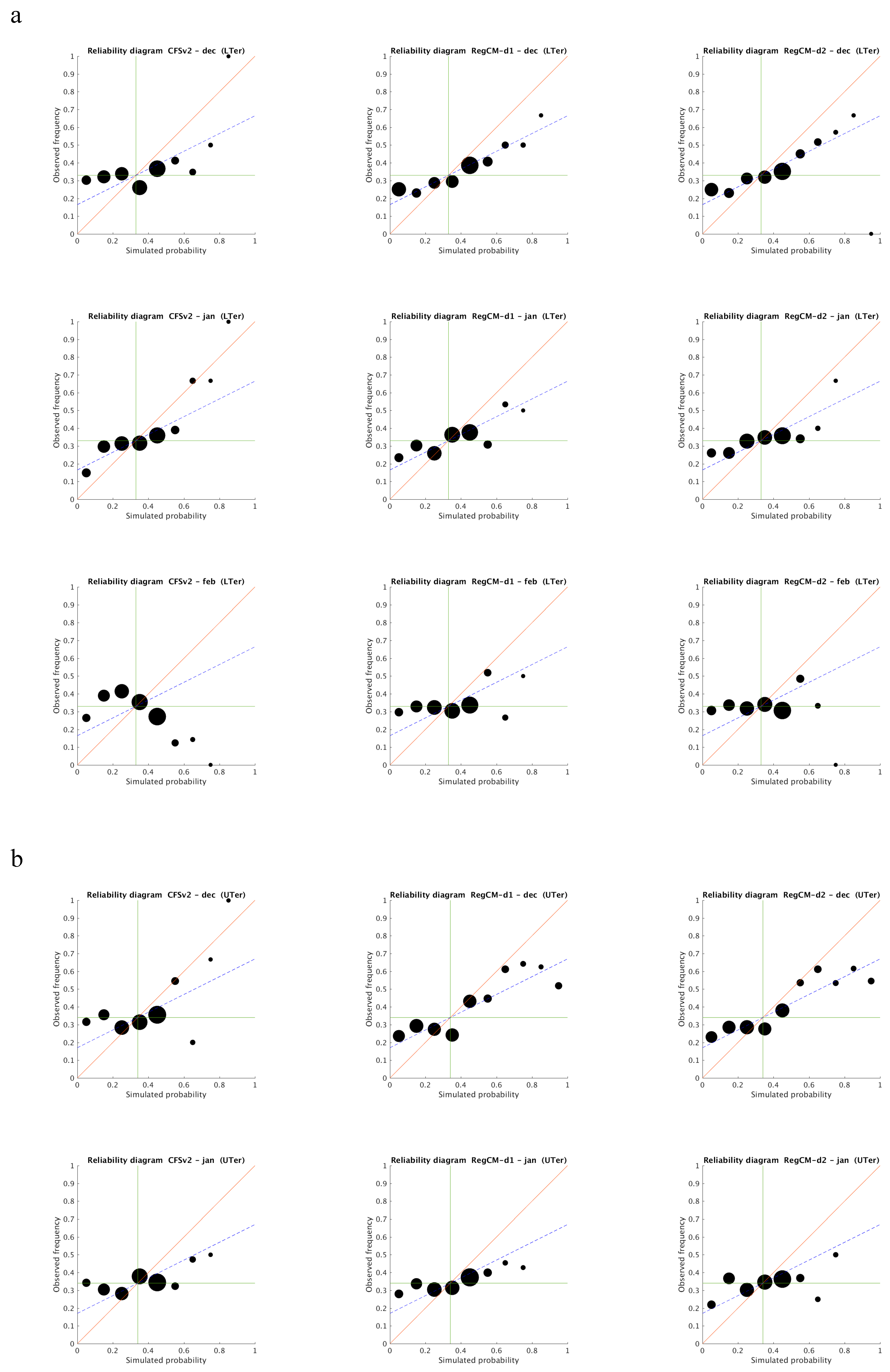
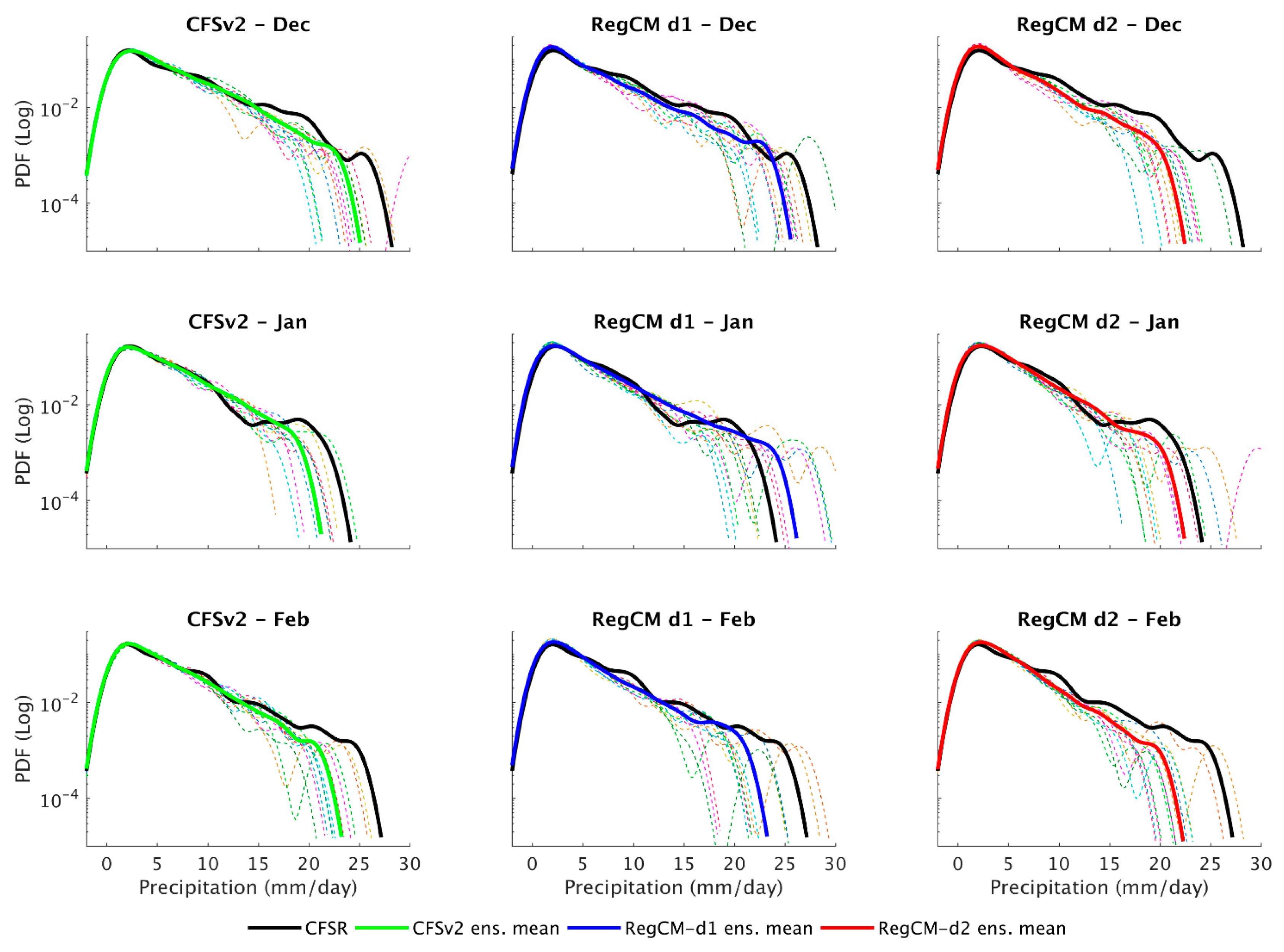
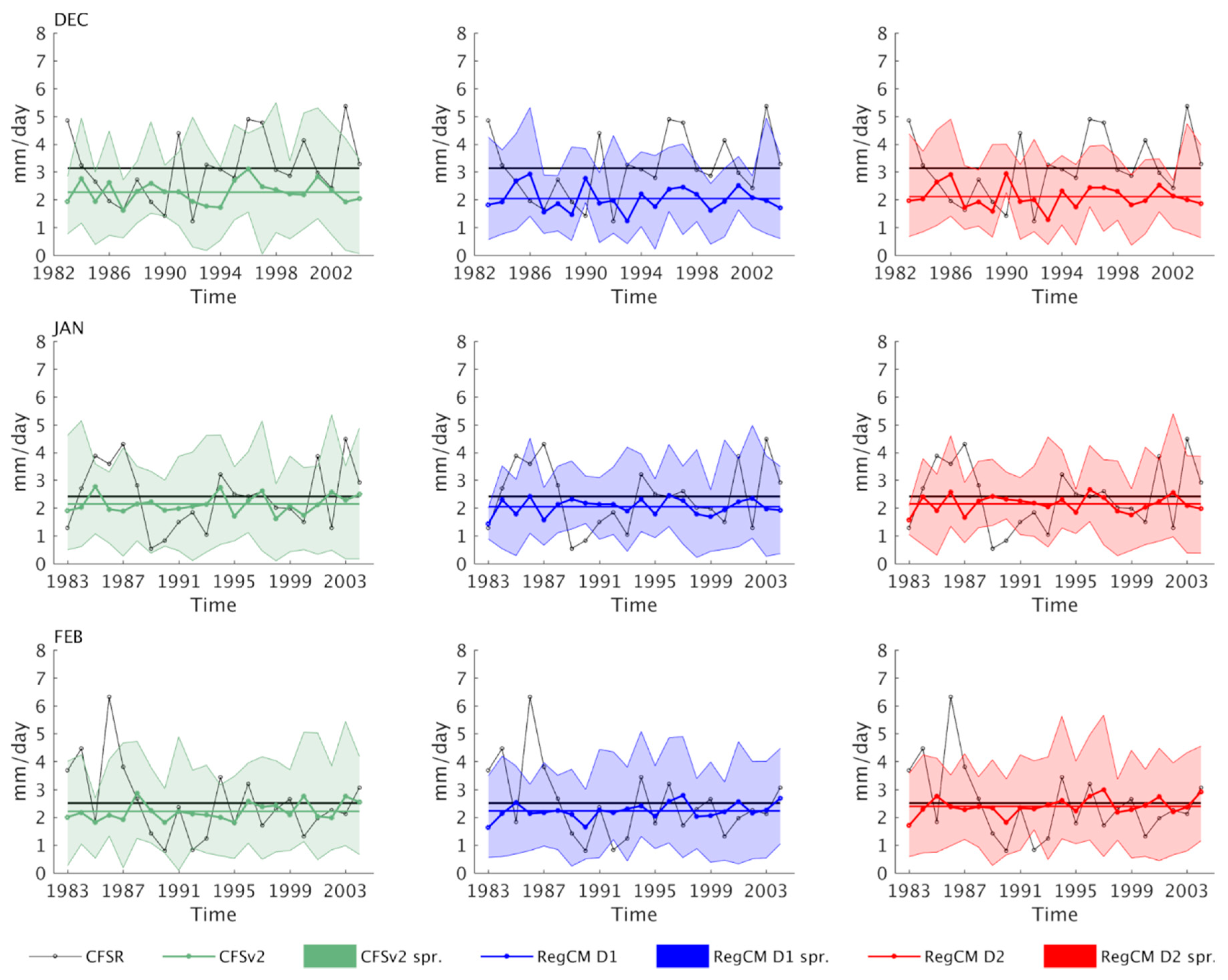
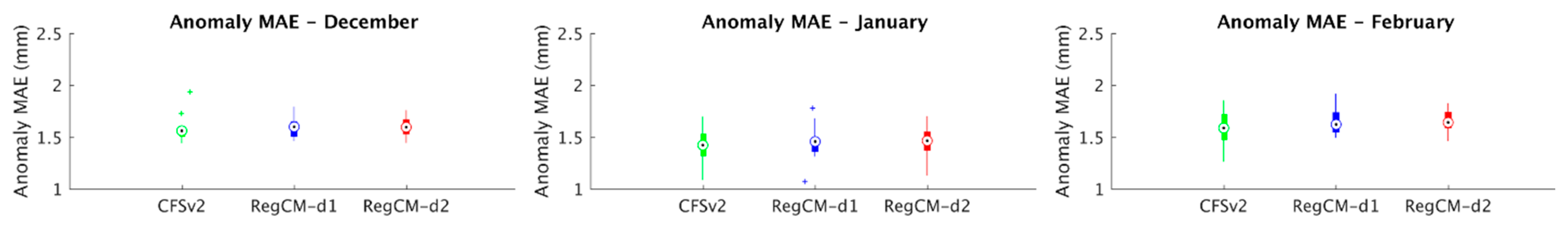
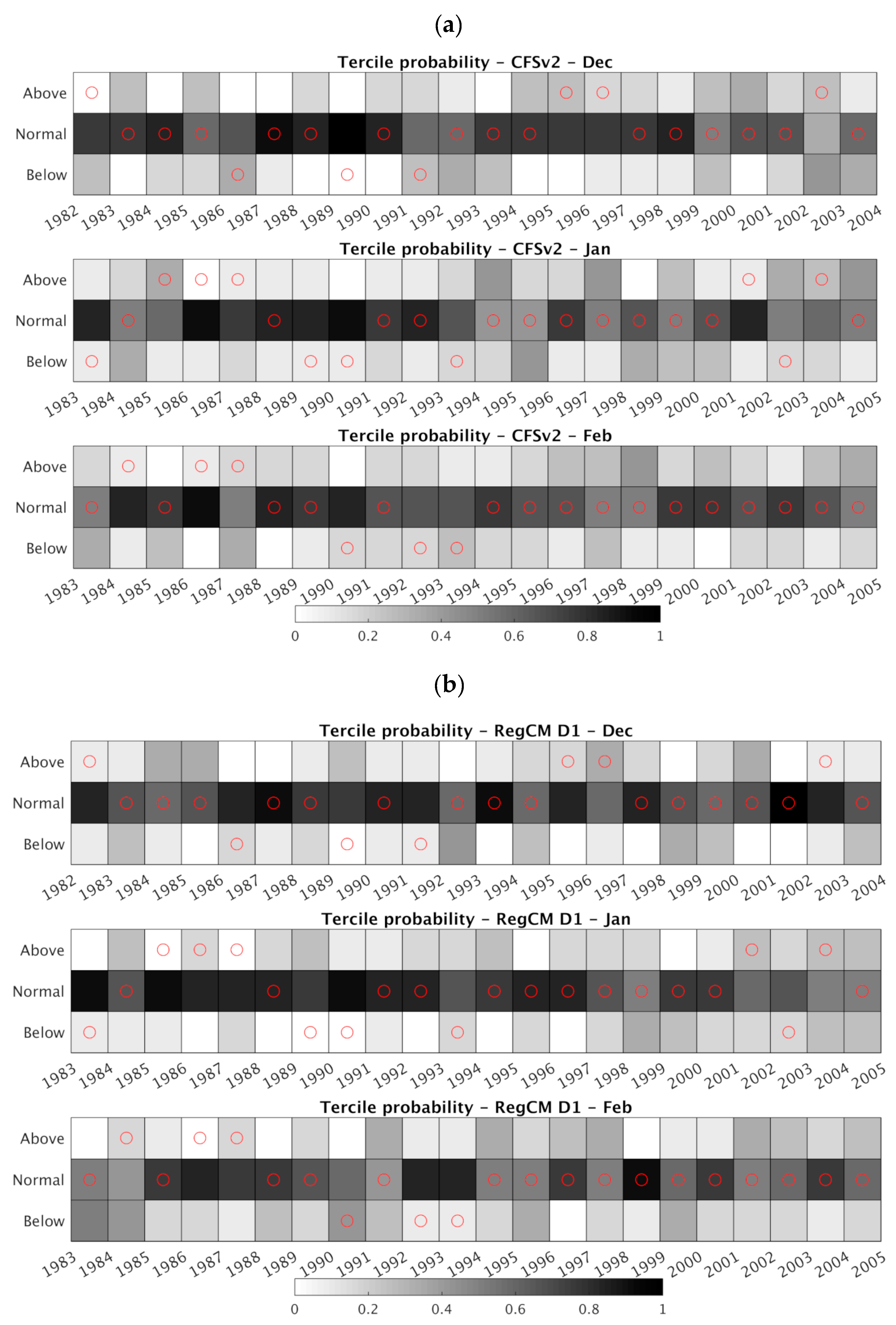
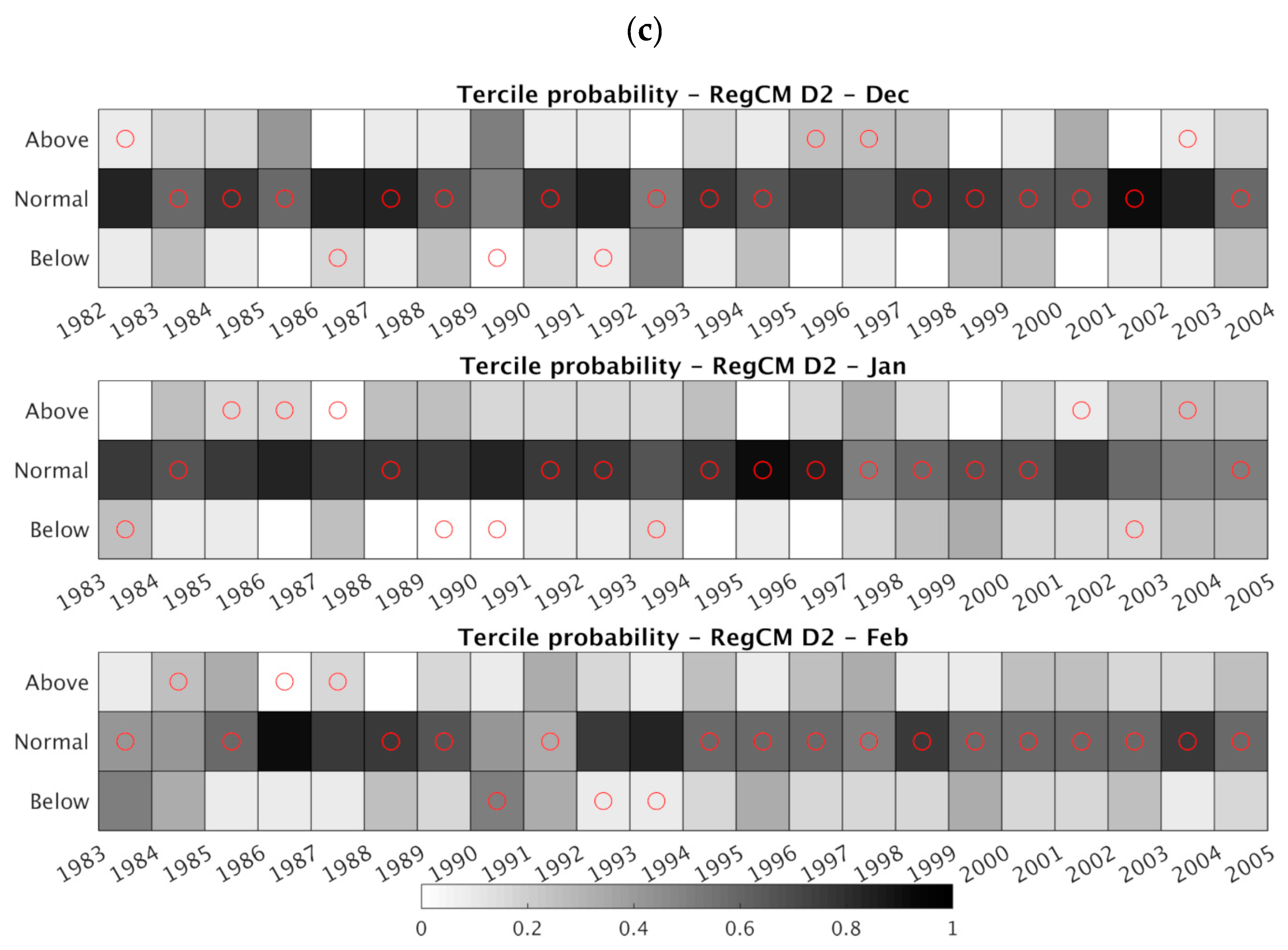
3.2. Precipitation Assessment
4. Summary and Conclusions
Author Contributions
Acknowledgments
Conflicts of Interest
References
- Kumar, A. On the assessment of the value of the seasonal forecast information. Meteorol. Appl. 2010, 17, 385–392. [Google Scholar] [CrossRef]
- Goddard, L.; Mason, S.J.; Zebiak, S.E.; Ropelewski, C.F.; Basher, R.; Cane, M.A. Current approaches to seasonal-to-interannual climate predictions. Int. J. Climatol. 2001, 21, 1111–1152. [Google Scholar] [CrossRef]
- Alexander, M.A.; Bladé, I.; Newman, M.; Lanzante, J.R.; Lau, N.C.; Scott, J.D. The atmospheric bridge: The influence of ENSO teleconnections on air-sea interaction over the global oceans. J. Clim. 2002, 15, 2205–2231. [Google Scholar] [CrossRef]
- Grassi, B.; Redaelli, G.; Visconti, G. Evidence for tropical sst influence on antarctic polar atmospheric dynamics. Geophys. Res. Lett. 2009, 36, 1–5. [Google Scholar] [CrossRef]
- Manzanas, R.; Frías, M.D.; Cofiño, A.S.; Gutiérrez, J.M. Validation of 40 year multimodel seasonal precipitation forecasts: The role of enso on the global skill. J. Geophys. Res. 2014, 119, 1708–1719. [Google Scholar] [CrossRef]
- Stockdale, T.N.; Anderson, D.L.T.; Balmaseda, M.A.; Doblas-Reyes, F.; Ferranti, L.; Mogensen, K.; Palmer, T.N.; Molteni, F.; Vitart, F. ECMWF seasonal forecast system 3 and its prediction of sea surface temperature. Clim. Dyn. 2011, 37, 455–471. [Google Scholar] [CrossRef]
- Mariotti, A.; Zeng, N.; Lau, K.M. Euro-Mediterranean rainfall and ENSO-a seasonally varying relationship. Geophys. Res. Lett. 2002, 29, 2–5. [Google Scholar] [CrossRef]
- Grassi, B.; Redaelli, G.; Visconti, G. Arctic sea ice reduction and extreme climate events over the mediterranean region. J. Clim. 2013, 26, 10101–10110. [Google Scholar] [CrossRef]
- Mishra, N.; Prodhomme, C.; Guemas, V. Multi-model skill assessment of seasonal temperature and precipitation forecasts over Europe. Clim. Dyn. 2019, 52, 4207–4225. [Google Scholar] [CrossRef]
- Ineson, S.; Scaife, A.A. The role of the stratosphere in the European climate response to El Nĩo. Nat. Geosci. 2009, 2, 32–36. [Google Scholar] [CrossRef]
- Marshall, A.G.; Scaife, A.A. Impact of the QBO on surface winter climate. J. Geophys. Res. Atmos. 2009, 114, 2–7. [Google Scholar] [CrossRef]
- Saha, S.; Nadiga, S.; Thiaw, C.; Wang, J.; Wang, W.; Zhang, Q.; Van den Dool, H.M.; Pan, H.L.; Moorthi, S.; Behringer, D.; et al. The NCEP Climate Forecast System. J. Clim. 2006, 19, 3483–3517. [Google Scholar] [CrossRef] [Green Version]
- Molteni, F.; Stockdale, T.; Balmaseda, M.; Balsamo, G.; Buizza, R.; Ferranti, L.; Magnusson, L.; Mogensen, K.; Palmer, T.; Vitart, F. The New ECMWF Seasonal Forecast System (System 4). ECMWF Tech. Memo. 2011, 656, 49. [Google Scholar]
- Maclachlan, C.; Arribas, A.; Peterson, K.A.; Maidens, A.; Fereday, D.; Scaife, A.A.; Gordon, M.; Vellinga, M.; Williams, A.; Comer, R.E.; et al. Global Seasonal forecast system version 5 (GloSea5): A high-resolution seasonal forecast system. Q. J. R. Meteorol. Soc. 2015, 141, 1072–1084. [Google Scholar] [CrossRef]
- Voldoire, A.; Sanchez-Gomez, E.; Salas y Mélia, D.; Decharme, B.; Cassou, C.; Sénési, S.; Valcke, S.; Beau, I.; Alias, A.; Chevallier, M.; et al. The CNRM-CM5.1 global climate model: Description and basic evaluation. Clim. Dyn. 2013, 40, 2091–2121. [Google Scholar] [CrossRef]
- Cherchi, A.; Fogli, P.G.; Lovato, T.; Peano, D.; Iovino, D.; Gualdi, S.; Masina, S.; Scoccimarro, E.; Materia, S.; Bellucci, A.; et al. Global Mean Climate and Main Patterns of Variability in the CMCC-CM2 Coupled Model. J. Adv. Model. Earth Syst. 2019, 11, 185–209. [Google Scholar] [CrossRef]
- Sangelantoni, L.; Russo, A.; Gennaretti, F. Impact of bias correction and downscaling through quantile mapping on simulated climate change signal: A case study over Central Italy. Theor. Appl. Climatol. 2019, 135, 725–740. [Google Scholar] [CrossRef]
- Diro, G.T.; Tompkins, A.M.; Bi, X. Dynamical downscaling of ECMWF Ensemble seasonal forecasts over East Africa with RegCM3. J. Geophys. Res. Atmos. 2012, 117, 1–20. [Google Scholar] [CrossRef]
- Ogwang, B.A.; Chen, H.; Li, X.; Gao, C. The Influence of Topography on East African October to December Climate: Sensitivity Experiments with RegCM4. Adv. Meteorol. 2014, 2014, 1–14. [Google Scholar] [CrossRef]
- Phan Van, T.; Van Nguyen, H.; Trinh Tuan, L.; Nguyen Quang, T.; Ngo-Duc, T.; Laux, P.; Nguyen Xuan, T. Seasonal Prediction of Surface Air Temperature across Vietnam Using the Regional Climate Model Version 4.2 (RegCM4.2). Adv. Meteorol. 2014, 2014, 1–13. [Google Scholar] [CrossRef]
- Siegmund, J.; Bliefernicht, J.; Laux, P.; Kunstmann, H. Toward a seasonal precipitation prediction system for West Africa: Performance of CFSv2 and high-resolution dynamical downscaling. J. Geophys. Res. 2015, 120, 7316–7339. [Google Scholar] [CrossRef]
- Díez, E.; Orfila, B.; Frías, M.D.; Fernández, J.; Cofiño, A.S.; Gutiérrez, J.M. Downscaling ECMWF seasonal precipitation forecasts in Europe using the RCA model. Tellus Ser. A Dyn. Meteorol. Oceanogr. 2011, 63, 757–762. [Google Scholar]
- Patarčić, M.; Branković, Č. Skill of 2-m Temperature Seasonal Forecasts over Europe in ECMWF and RegCM Models. Mon. Weather Rev. 2011, 140, 1326–1346. [Google Scholar] [CrossRef]
- Bedia, J.; Golding, N.; Casanueva, A.; Iturbide, M.; Buontempo, C.; Gutiérrez, J.M. Seasonal predictions of Fire Weather Index: Paving the way for their operational applicability in Mediterranean Europe. Clim. Serv. 2018, 9, 101–110. [Google Scholar] [CrossRef]
- Messeri, G.; Benedetti, R.; Crisci, A.; Gozzini, B.; Rossi, M.; Vallorani, R.; Maracchi, G. A new framework for probabilistic seasonal forecasts based on circulation type classifications and driven by an ensemble global model. Adv. Sci. Res. 2018, 15, 183–190. [Google Scholar] [CrossRef]
- Giorgi, F.; Lionello, P. Climate change projections for the Mediterranean region. Glob. Planet. Chang. 2008, 63, 90–104. [Google Scholar] [CrossRef]
- Giorgi, F.; Mearns, L.O. Introduction to special section: Regional Climate Modeling Revisited. J. Geophys. Res. 1999, 104, 6335. [Google Scholar] [CrossRef]
- Giorgi, F.; Coppola, E.; Solmon, F.; Mariotti, L.; Sylla, M.B.; Bi, X.; Elguindi, N.; Diro, G.T.; Nair, V.; Giuliani, G.; et al. RegCM4: Model description and preliminary tests over multiple CORDEX domains. Clim. Res. 2012, 52, 7–29. [Google Scholar] [CrossRef]
- Pal, J.S.; Small, E.E.; Eltahir, E.A.B. Simulation of regional-scale water and energy budgets: Representation of subgrid cloud and precipitation processes within RegCM. J. Geophys. Res. Atmos. 2000, 105, 29579–29594. [Google Scholar] [CrossRef]
- Grell, G. Prognostic evaluation of assumption used by cumulus parameterizations. Mon. Weather Rev. 1991, 121, 764–787. [Google Scholar] [CrossRef]
- Arakawa, A.; Schubert, W.H. Interaction of a cumulus cloud ensemble with the large-scale environment, part I. J. Atmos. Sci. 1974, 31, 674–701. [Google Scholar] [CrossRef]
- Zeng, X.B. Intercomparison of six bulk aerodynamic algorithms for the computation of sea surface fluxes. Ninth Conf. Interact. Sea Atmos. 1998, 226–229. [Google Scholar]
- Dickinson, R.; Errico, R.; Giorgi, F.; Bates, G. A regional climate model for the western United States. Clim. Chang. 1989, 15, 383–422. [Google Scholar] [CrossRef]
- Emanuel, K. A Scheme for Representing Cumulus Convection in Large-Scale Models. J. Atmos. Sci. 1991, 2313–2335. [Google Scholar] [CrossRef]
- Saha, S.; Moorthi, S.; Wu, X.; Wang, J.; Nadiga, S.; Tripp, P.; Behringer, D.; Hou, Y.; Chuang, H.; Iredell, M.; et al. The NCEP Climate Forecast System Version 2. J. Clim. 2014, 3, 2185–2208. [Google Scholar] [CrossRef]
- Saha, S.; Moorthi, S.; Wu, X.; Wang, J.; Nadiga, S.; Tripp, P.; Behringer, D.; Hou, Y.; Chuang, H.; Iredell, M.; et al. The NCEP Climate Forecast system reanalysis. Am. Meteorol. Soc. 2010, 16, 1015–1058. [Google Scholar] [CrossRef]
- Jolliffe, I.T.; Stephenson, D.B. Forecast Verification A Pratictioner’s Guide in Atmospheric Science; John Wiley & Sons Ltd: Chichester, UK, 2003; ISBN 0470864419. [Google Scholar]
- Weisheimer, A.; Palmer, T.N. On the Reliability Seasonal Climate Forecasts. Bull. Am. Meteorol. Soc. 2013, 62, 1654. [Google Scholar] [CrossRef]
- Manzanas, R.; Gutiérrez, J.M.; Fernández, J.; van Meijgaard, E.; Calmanti, S.; Magariño, M.E.; Cofiño, A.S.; Herrera, S. Dynamical and statistical downscaling of seasonal temperature forecasts in Europe: Added value for user applications. Clim. Serv. 2018, 9, 44–56. [Google Scholar] [CrossRef]
- Nikulin, G.; Asharaf, S.; Magariño, M.E.; Calmanti, S.; Cardoso, R.M.; Bhend, J.; Fernández, J.; Frías, M.D.; Fröhlich, K.; Früh, B.; et al. Dynamical and statistical downscaling of a global seasonal hindcast in eastern Africa. Clim. Serv. 2018, 9, 72–85. [Google Scholar] [CrossRef]
- Skamarock, W.C.; Klemp, J.B. A time-split nonhydrostatic atmospheric model for weather research and forecasting applications. J. Comput. Phys. 2008, 227, 3465–3485. [Google Scholar] [CrossRef]
- Kosovelj, K.; Kucharski, F.; Molteni, F.; Žagar, N. Modal Decomposition of the Global Response to Tropical Heating Perturbations Resembling MJO. J. Atmos. Sci. 2019, 76, 1457–1469. [Google Scholar] [CrossRef]


| Mean-MAE | 5p-MAE | 50p-MAE | 95p-MAE | Inter-Annual Anomaly-MAE | |
|---|---|---|---|---|---|
| CFSv2 | 1.7 | 2.2 | 1.7 | 1.5 | 1.8 ± 0.20 |
| RegCM-d1 | 1.4 | 1.7 | 1.4 | 1.4 | 1.5 ± 0.19 |
| RegCM-d2 | 0.8 | 1.0 | 0.8 | 0.8 | 1.5 ± 0.20 |
| Mean-MAE | 50p-MAE | 95p-MAE | Inter-Annual Anomaly-MAE | |
|---|---|---|---|---|
| CFSv2 | 0.7 | 0.2 | 3.2 | 1.5 ± 0.16 |
| RegCM-d1 | 0.6 | 0.2 | 3.4 | 1.5 ± 0.13 |
| RegCM-d2 | 0.8 | 0.2 | 4.6 | 1.5 ± 0.12 |
© 2019 by the authors. Licensee MDPI, Basel, Switzerland. This article is an open access article distributed under the terms and conditions of the Creative Commons Attribution (CC BY) license (http://creativecommons.org/licenses/by/4.0/).
Share and Cite
Sangelantoni, L.; Ferretti, R.; Redaelli, G. Toward a Regional-Scale Seasonal Climate Prediction System over Central Italy Based on Dynamical Downscaling. Climate 2019, 7, 120. https://doi.org/10.3390/cli7100120
Sangelantoni L, Ferretti R, Redaelli G. Toward a Regional-Scale Seasonal Climate Prediction System over Central Italy Based on Dynamical Downscaling. Climate. 2019; 7(10):120. https://doi.org/10.3390/cli7100120
Chicago/Turabian StyleSangelantoni, Lorenzo, Rossella Ferretti, and Gianluca Redaelli. 2019. "Toward a Regional-Scale Seasonal Climate Prediction System over Central Italy Based on Dynamical Downscaling" Climate 7, no. 10: 120. https://doi.org/10.3390/cli7100120
APA StyleSangelantoni, L., Ferretti, R., & Redaelli, G. (2019). Toward a Regional-Scale Seasonal Climate Prediction System over Central Italy Based on Dynamical Downscaling. Climate, 7(10), 120. https://doi.org/10.3390/cli7100120