Article

Prospective Climate Change Impacts upon Energy Prices in the 21ST Century: A Case Study in Italy

by
Giovanni Martino Bombelli
,
Andrea Soncini
,
Alberto Bianchi
and
Daniele Bocchiola
*
Department of Civil and Environmental Engineering DICA, Politecnico di Milano, l. da Vinci 32, 20133 Milano, Italy
*
Author to whom correspondence should be addressed.
Climate 2019, 7(10), 121; https://doi.org/10.3390/cli7100121
Submission received: 5 September 2019 / Revised: 30 September 2019 / Accepted: 14 October 2019 / Published: 15 October 2019
(This article belongs to the Special Issue Climate Change, Carbon Budget and Energy Policy)

Abstract

:
The assessment of the effect of the electricity price on energy production is important when studying the profitability and benefits of energy systems. The demand and price of electricity depends upon societal and economic development, but it is subject to a seasonal, weather-dependent variability, and possibly to long-term variation under climate change. Here, we developed a methodology to model the energy demand and electricity price in response to gross domestic product (GDP), temperatures, and random factors, usable for the purpose of cost/benefit analysis of production systems. The method was applied to the case study of the Italian electricity market, showing acceptable capacity of modelling recently observed price fluctuations. Then, we gathered climate projections until 2100 from three global climate models of the IPCC AR5, under RCP2.6, RCP4.5, and RCP8.5, and we produced future scenarios of price fluctuations for two reference decades, half-century 2040–2049, and end-of-century 2090–2099. Our scenarios displayed a potential for the reduction of energy demand in winter, and an increase in summer and spring, and for the similarly-changing electricity price throughout the 21st century. We discuss the application of our model with the specific aim of the projection of future hydropower production, as controlled by climate, hydrology, demand, and price constraints, with examples from recent studies. Our results provide a tool for modelling the behaviour of energy systems based upon knowledge of external factors, usable for further investigation of energy systems, such as hydropower, and others, taking into account the key variables affecting energy production and energy price.

1. Introduction

Energy demand and pricing are affected by climate change, and production is thereby impacted. A most sensitive sector is hydropower. Recently, the effect of climate change on hydrological regimes [1,2], and on the related production of hydroelectric energy, especially from high altitude water bodies and reservoirs, has been the subject of several studies [3].
A most important issue is the change of the price and demand for electricity, the latter being visibly influenced by meteorological changes, as recently evidenced, e.g., by Gaudard [4] under the umbrella of the project “Assessing Climate impacts on the Quantity and quality of Water”, AQWA [5]. In fact, at the European level, hydropower is still one of the main renewable energy sources, accounting for ca. 15% of total capacity, i.e., about 141 GW [6]. The average net energy produced by European hydroelectric plants is nearby 569 TWh yearly. At the country level, Russia is first in Europe, and fifth in the world rankings with 52 GW, second is Norway with 31 GW, and France follows with 25 GW. Italy, with an installed capacity of 22.5 GW of hydropower, is fourth in Europe, and 11th worldwide. In Italy hydroelectric plants, 3700 units, achieved a total production of 42.4 TWh, ca. 14% of the country’s production. Most such plants are small, and have marginal influence. In fact, in 2015, 77% of Italian hydropower was produced by plants with power >10 MW, covering merely 17% of the total [7].
However, hydropower energy depends largely upon meteorological conditions and, therefore, productivity can have significant variations seasonally, and from year to year. Climate conditions influence (i) the hydrological cycle, (ii) the energy demand, and (iii) the electricity price, the latter two especially depending upon temperature. These three factors influence hydroelectric production because energy managers need to manage water storages, so as to cover periods of peaking electricity prices resulting from high energy demand, to reach the goal of maximum profit.
The average annual temperatures in Italy grew by +1.7 °C since the end of the 17th century, but the most relevant contribution to this increase was recorded in the latest 50 years, with an increase of about +1.4 °C [8]. Additionally, in a study carried by ISPRA (Higher Institute for Environmental Protection and Research of Italy) [9], based upon 140 meteorological stations, the average temperature decreased in Italy during 1961–1981, with a subsequent increase until 2008, for a net increase of ca. +1 °C.
Given the impact of climate upon the energy market as examined here, one needs to investigate the present and potential future effect of climate, and climate change, on energy systems. One can do so by applying models of the energy market explicitly depending upon weather variables.
Several models aimed at estimating the electricity prices were recently introduced in Europe in the wake of the liberalization of the energy market at the end of the 1990s. Such liberalization brought to the country-wise definition of the free market as indicated by Weron [10]. In Italy the Legislative Decree 79/99, also called Decreto Bersani, allowed such liberalization.
As indicated, e.g., by Weron [10], in the available literature there are various types of models for estimating electricity prices [11], and some categories can be highlighted, however, arbitrarily, and prone to some overlapping.
A first category is given by multi-agent models. Agents are defined as entities able to reproduce the behaviour of (parts of) the system, pending specific tuning [12]. Such models are flexible in studying the interactions between various components, but they require strong functional assumptions, possibly limiting the field of application. In parametric models, the progress of the system is described via some operators (e.g., black-box type), that accounts for different responses against different inputs, and need parameters’ tuning against data. Given the large number of parameters required for the depiction of complex systems, more compact models have been developed, such as the supply curve, described by Kanamura and Ohashi [13], linking the energy demand to the energy price, with use of functions previously calibrated, e.g., on a daily basis.
These models may be strongly limited by the possibly very high number of samples necessary for tuning. In addition, they lack in considering the potential for stochastic (random) fluctuations in the energy systems, not foreseeable deterministically. To deal with such issues, stochastic models may be used. These models derive future electricity prices using a combination of previous (past) prices, by applying statistical methods, mostly based on regressive or self-regressive assumptions (AR, ARX, GARCH) [14,15,16]. The accuracy of the forecast depends on the quality of the data available, and on the ability to incorporate the different factors affecting the process and the forecast.
Another important category is given by computational models [17], able to consider the large non-linearity of the system, e.g., using neural networks. These methods normally achieve good results in the short-term, and their performance depends on the calibration data and periods. Hybrid, or mixed, models can be also developed. As an instance, the s-MTSIM model by RSE [18] is made of two components (stochastic/heuristic), and it is derived from the existing deterministic Medium-Terms power system Simulator (MTSIM), originally developed by RSE SpA.
This latter model was applied, e.g., in the GridTech project, “Innovative grid-impacting technologies enabling a clean, efficient and secure electricity system in Europe”, which was supported by the Intelligent Energy Europe Programme (IEE). The main objective of GridTech was the performance of an assessment of new grid-impacting technologies (e.g., solar, wind, etc.), and their implementation into the European electricity system. This would allow a comparison of different technological options, towards the exploitation of the full potential of future electricity production from renewable energy sources (RES-E), with the lowest possible total energy system cost. The time window considered in the GridTech analyses was until 2050, with special consideration of the target years 2020, 2030 and 2050, each one under a scenario of energy demand and electricity price.
Another work of interest is the e-Highway2050 project [19], launched from a European consortium supported by the EU Seventh Framework Programme (FP7), and devoted to develop a long-term planning methodology for the expansion and restructuring of European electricity transmission grids until 2050. The project consortium, involving some partners on the Italian side, is examining conditions and solutions for the planning of the European electricity grid until 2030, 2040 and 2050, based on energy demand forecasting for different scenarios.
An additional example is given by ClimateCost, a project with the objective to describe the impacts and the costs of climate change in the European energy system. The consortium therein elaborated the POLES model [20], a market-oriented model that can define the equilibrium price for several energy sources, simulating the energy system behaviour.
Here, we propose a simplified hybrid method that can be applied in developing future projections of electricity price and energy demand according to future scenarios of climate change. The model, general in its nature, can be used henceforth for the benchmarking of adaptation measures for energy production, and most notably for hydropower [21], under potentially variable climate in the future.
The manuscript is organized as follows: In the section “Case Study” we quickly describe the main features of the Italian energy system, of interest for our work. In the section “Methods” we depict the methodology, and in the “Data” section we describe the database used here. In the section “Results”, we demonstrate the accuracy of our method for the Italian energy market, and we display the projected evolution therein under climate change scenarios. In the section “Discussion”, we benchmark our results against findings from recent studies, and we discuss the application of our model for the specific aim of assessing hydropower production. We then draw some conclusions and outline possible future efforts.

2. Case Study

Our method will be applied to the Italian electricity system. Such a system is made of a network, where different activities are carried out by different subjects, within a free energy market environment.
Such activities cover production, transmission, and distribution of electricity, subject to various technical constraints (i.e., limitations in energy distribution, node-limited grid capacity). Non-compliance with such constraints, even when limited in time, can produce rapid system crises. The electric power fed into the network is not traceable, so that every local imbalance falls out upon the network through variations in voltage and frequency.
The main issues affecting proper supply are given by (i) the variability, poor elasticity and limited predictability of demand, (ii) the absence of storage capacity, and (iii) the dynamic change of the technical constraints, in response to real market adjustment.
Management of the electricity market is entrusted to the Gestore dei Mercati Energetici (Energy Markets Operator, herein GME), with the mission of promoting the development of a national competitive electricity system, according to the criteria of neutrality, transparency and objectivity. The electricity market is particularly sensitive to these criteria.
Competition in the electricity market is introduced via the action of Borsa Elettrica, an electricity stock market. It promotes the application of efficient equilibrium prices, allowing the sale and purchase of electricity according to the greater economic convenience. It is organised as a real physical market, with the definition of sales and purchases through hourly charts, according to the criterion of economic merit. This consists of considering, for sales, the prices in increasing order and, for purchases, the prices in decreasing order. Price definition takes place by all means as in a physical market, according to matching of supply and demand. Electricity offers are accepted in order of economic merit, i.e., in order of increasing price, until their sum in terms of kWh completely meets the demand.
The kWh price of the last accepted bidder, i.e., the one with the highest price, is attributed to all offers, and according to European Directive 2009/28, renewable energies, like hydropower, have priority in terms of access to the market.
In so doing, in each zone of the Italian territory with given technical constraints, the equilibrium prices are defined, i.e., those that are found at the intersection of the supply and demand curves. Subsequently, the Prezzo Unico Nazionale (PUN, National Single Price), which is the Italian electric energy market index, is established by GME. This represents the average selling price, weighed on total purchases, and it is a result of different auctions, in which GME covers the expected energy demand hour by hour, with offers by various operators. The auction accepts, first, the cheapest energy offers, and then the most expensive to cover the needs of that particular hour, and the price applied to all the operators is that of the most expensive source selected.
As a mere example, we could hypothesize to have a market made of three operators, each one producing 1 MWh of energy, each one with a different price, say of 10, 20 and 30 €/MWh, and a total energy demand of the market of 2 MWh. In this case, the chosen operators would be those pricing energy at 10 and 20 €/MWh, i.e., the most advantageous. The price at which the energy would be paid, i.e., PUN, is 20 €/MWh, that is, from the most expensive source selected.
In this work the PUN, which is defined for each hour of every day on the basis of the match between supply and demand, is also called the Electricity Price, given that a homogenous price distribution is met, in practice, in the whole Italian territory.

3. Methods

3.1. Energy Demand Model

Electricity prices are strongly dependent on the energy demand. Thus, projections of future electricity price require a model of such demand. Energy demand is also influenced by meteorological variables, most notably temperature, influencing heating (winter) and cooling (summer) needs. In some previous works (e.g., Shourav [22]) the influence of precipitation was also considered, but the correlation with energy demand was weak.
In the field of energy study, the dependence on the mean daily temperature can be described by defining two variables, namely Heating Degree Day (HDD), and Cooling Degree Day (CDD) ([23,24,25]). These factors describe the heating and cooling need, occurring when the temperature deviates from thresholds, defined as τH and τC, respectively”
{ HDD ( d ) = min ( ( T ( d ) τ H ) , 0 ) CDD ( d ) = max ( ( T ( d ) τ C ) , 0 )
where T(d) (°C) is the average daily temperature at day d. Another input of the energy demand model is the annual gross domestic product GDPy, given that a large base request of energy comes from industrial users.
Accordingly, one can hypothesize that the demand on a specific year y, and a specific day d can be modelled using a power law, expressed in a log-log form as:
ln ( D d ) y = α ln ( GDP y ) + β ln ( HDD d + 1 ) + γ ln ( CDD d + 1 ) + i = 1 4 δ i + ε d
where Dd (GWh) is the daily energy demand, α, β, and γ are tuning parameters, δi are tuning factors for Saturdays (i = 1), Sundays (i = 2), holidays (i = 3) and vacation periods (i = 4), including the Christmas holiday period, Easter period and August central weeks. The term εd is a random Gaussian error, accounting for random factors. This equation does not account for change in energy policies, or different behaviour of consumers (e.g., large use of domestic power systems, solar panels, etc.), but only includes the impact of climate on demand.

3.2. Electricity Price Model

The electricity price model is hybrid, and it mixes a parametric model, and a probabilistic one to model hourly energy price at time t as:
P ( t ) = e g ( t ) + x ( t ) = e g ( t ) e x ( t ) = G ( t ) e x ( t )
Here, P(t) (€MWh−1) is the hourly price. G(t) is the parametric, i.e., deterministic part of the model, and x(t) is the probabilistic part.
The deterministic part G(t) describes the hourly mean price, linked to the daily energy demand, while the probabilistic component describes the high intrinsic volatility of energy demand. The G(t) part estimates the hourly mean price from the daily mean energy demand D(t), as:
G ( t ) = [ exp ( δ t ) + exp ( α 0 + α 1 D t ) + exp ( i = 1 24 ( γ i | hour = i ) ) ] i = 1 2 ( η i | day = i )
Here, δ (h−1) is the base, time-dependent increase of price, while (α0 + α1Dt) describes the connection between price and mean daily energy demand D t . The α1 factor is α 1 = α 1 , 0 + α 1 , 1 t , representing the time-dependent response (increase/decrease) of prices, to changes in energy demand. The term i = 1 24 ( γ i | hour = i ) has 24 tuning parameters, γ i , necessary to define an hourly price, i.e., the difference between hourly, and daily mean. The terms η i are dummy factors applied to Sundays, and holidays. The statistical component aims at emulating the high intrinsic volatility of the system, with an autoregressive model AR ( 1 ) :
x ( t ) = a + b x ( t 1 ) + ϵ t
where a , e and b are tuning parameters, ϵ t N ( 0 , σ ϵ ) is a random Gaussian error, and x t 1 is the value of the component at the previous step.

4. Data

Historical Data and Future Scenarios

The input data available are (i) GDP ( t ) data series, provided by the Organisation for Economic Cooperation and Development (OECD), (ii) energy demand and price of electricity (PUN), provided by GME, and (iii) a series of mean daily temperature for Italy, provided by ISPRA [23]. Temperature data are used to assess HDD and CDD, at the national scale, as in the Equation (1). Accordingly, both of these parameters partly lose their physical, local meaning to instead represent generally valid model parameters, country-wise. Depending on data availability, and after a preliminary quality check, the reference period considered in the study covers 2005–2013. Using the annual GDP and the daily HDD and CDD, it is possible to evaluate the energy demand for each day in our period of reference, from which the hourly energy price in that period is evaluated. This value is then used for tuning our models in Section 5.1.
To project future energy demand, and electricity price on the Italian territory, we used data of (i) the OECD future projection of GDP, and (ii) the future projection of mean daily temperature series for Italy, from the IPCC (Intergovernmental Panel on Climate Change) scenarios.
Climate projections of temperature are given by different global circulation models (GCMs), under different representative concentration pathways (RCPs), as provided by the IPCC. The three chosen GCMs were taken from the Coupled Model Intercomparison Project release 5, CMIP5. These models are ECHAM6 (European Centre Hamburg Model), CCSM4 (Community Climate System Model), and EC-EARTH (European Consortium Earth System Model). The RCP scenarios are named RCP2.6 (optimistic, peak in radiative forcing at 3 Wm 2 or 490 ppm   CO 2 equivalent in 2040, and then decline to 2.6 Wm 2 ), RCP4.5 (cautious, stabilization without overshoot pathway to 4.5 Wm 2 , or 650 ppm   CO 2 equation, at 2070), and RCP8.5 (pessimistic, with rising radiative forcing up to 8.5 Wm 2 , or 1370 ppm   CO 2 equation by 2100). The temperature values from the GCMs’ grids were bias corrected monthly (i.e., by properly fixing their mean values) against historical data (2005–2013) [26], so obtaining for each RCP and each model a series of daily temperatures until 2100, for a grand total of nine scenarios.
Feeding these climate projections into our properly-tuned models, we pursued projections of energy demand and electricity price to assess the effect of the climate change upon the electricity system.

5. Results

5.1. Tuning of Energy Demand, and Price Model

The previously defined parametric models entail parameters that cannot be measured directly and, therefore, a tuning procedure was carried out, via linear regression on the logarithms. The two models were calibrated separately using observed values of the variables involved, and their accuracy was evaluated by objective scores, namely, the determination coefficient R2 and root mean square error (RMSE). The calibration was carried out during 01/01/2005–31/12/2010. The Italian electricity market started in April 2004, and data collected in the first period were not considered, to avoid disturbances during stabilization of the market. The database for calibration included daily (demand), and hourly (price) samples for six years, so the database was large enough to support linear regression with a large number of parameters as here (eight parameters for demand against 6 × 365 = 2190 daily values, and 33 parameters for price, against 6 × 365 × 24 = 52,560 hourly values). To set up the energy demand model, one needs first to fix the value of the temperature thresholds for cooling and heating in Equation (1), i.e., τH, τC, to be chosen within a plausible range from the literature [3,23]. We thus proceeded as follows:
We chose couples of τH, τC from within a pre-defined range (12–20 for τC, and 10–20 for τH), changing iteratively the values of τH, τC by 1 °C steps, and for each couple we pursued a linear regression (on the logs) procedure, to estimate the remaining model parameters in Equation (2). We then chose the couple providing the highest value of R2 (on the real values) of the regression. In so doing, we took the models’ parameters leading to the best fit of the observed demand data.
A best fit was obtained by τH = 18 °C and τC = 15 °C, giving R2 = 0.867 and RMSE = 2.163 GWh. We report in Table 1 the adaptation scores for calibration and validation (we report R2log, and R2 for completeness).
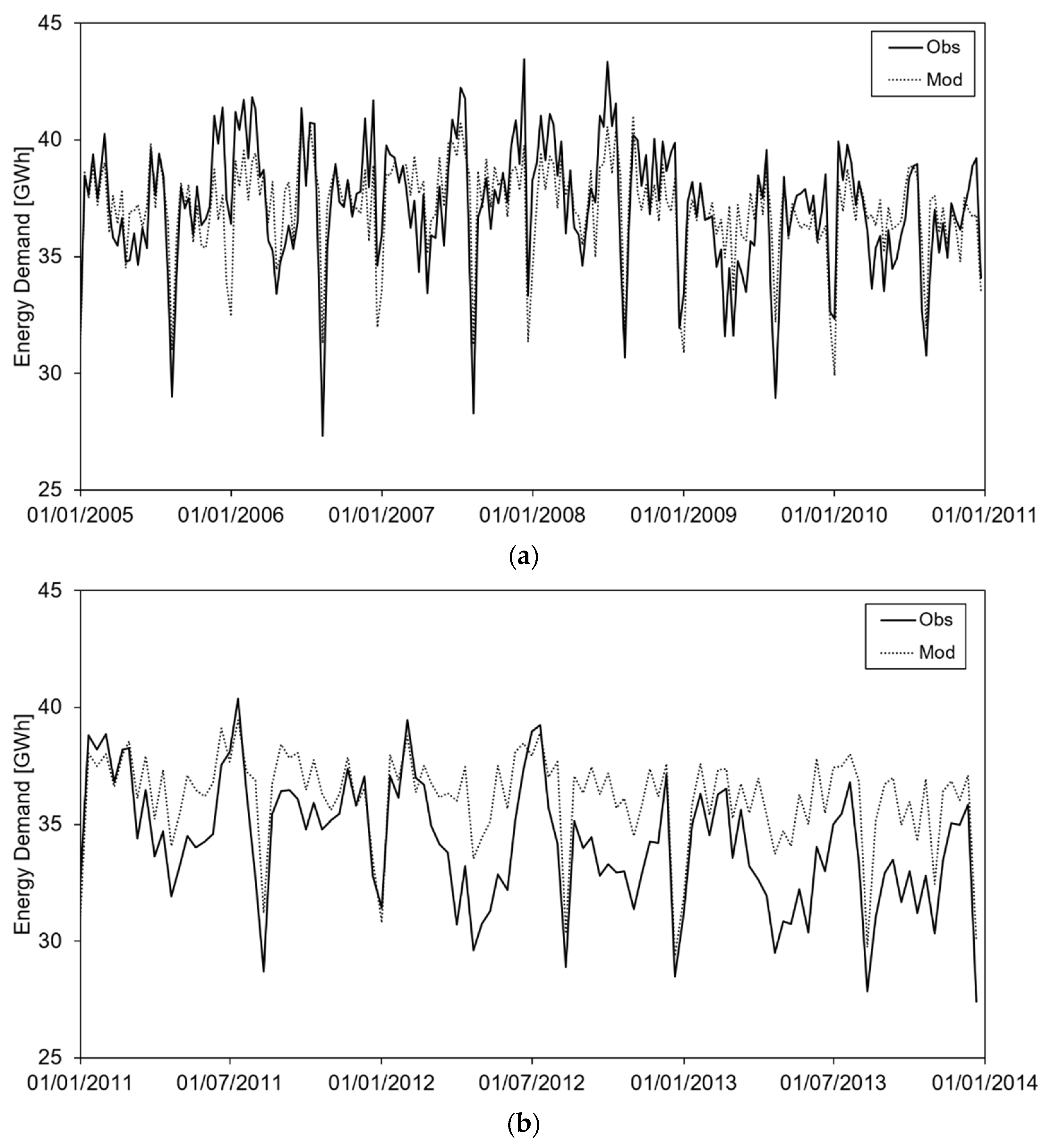
Figure 1a reports the mean energy demand during the calibration period, as per weekly mean values (the daily values are not reported, as they are difficult to interpret visually). Clearly from Figure 1a and Table 1, the model of energy demand fits acceptably the observation in the calibration phase, even capturing well enough the peak timing, albeit with some underestimation.
Validation was pursued against data during 2011–2013, also reported in Table 1. Figure 1b shows the weekly average values of energy demand in the validation period. We obtained scores of R2 = 0.583, and RMSE = 2.816 GWh, and Table 2 shows the estimated parameters for calibration of the energy demand model.
Table 2 shows the estimated parameters for calibration of the electricity price model, with scores R2 = 0.499, and RMSE = 25.04 €/MWh. Here, linear regression was pursued to simultaneously assess all parameters.
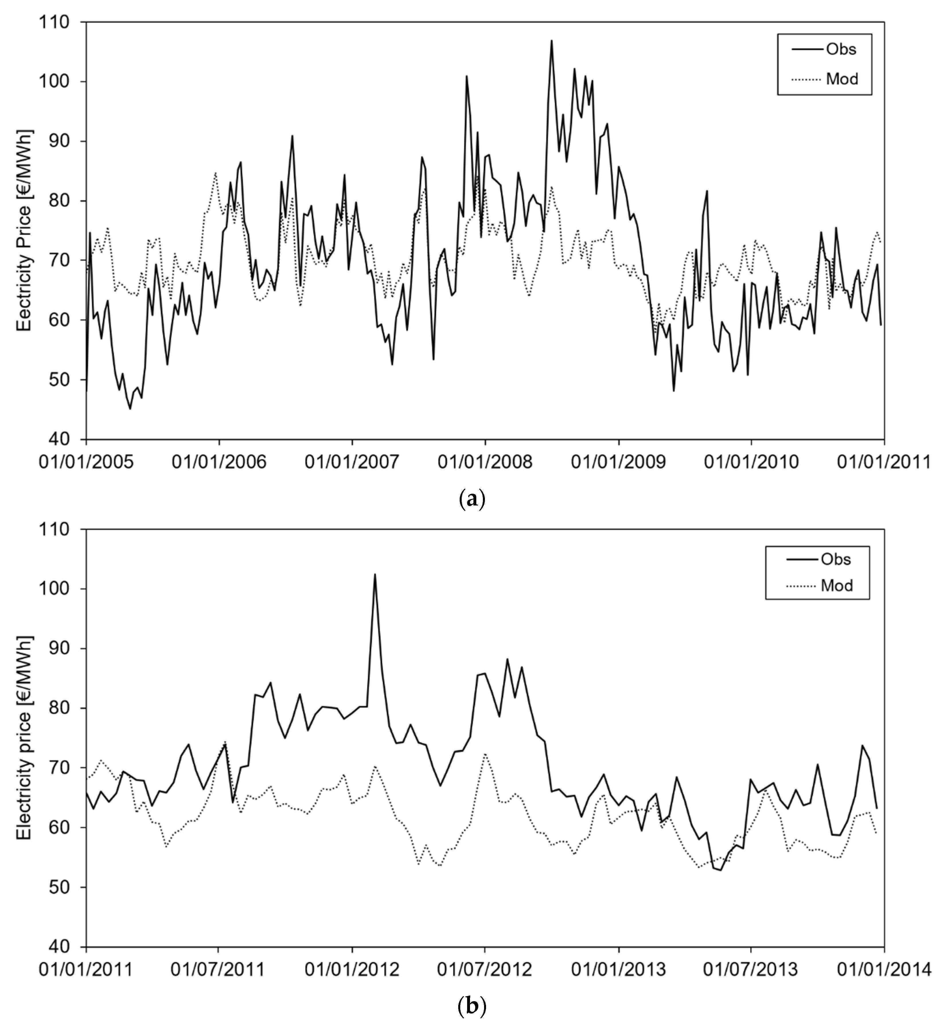
Figure 2a reports the (weekly mean) electricity price, modelled and observed, for the calibration period (again 2005–2010). In comparison with the energy demand model, the electricity price model has lower goodness of fit indices. This likely results from inelasticity of the system, requiring for simulation the insertion of a tool accounting for system volatility (i.e., chance, or random factors). Figure 2b reports model performance in the validation period. Here, the model scores are quite low: R2 = 0.063, and RMSE = 34.98 €/MWh.
In years 2011 and 2012 the price of oil exceeded the value of $100 per barrel, possibly affecting electricity price and the performance of our model. Oil price is, in most cases, the result of political decisions and, therefore, cannot be easily modelled (De Almeida and Silva, 2011 [27]).

5.2. Future Projections of Energy Demand and Price

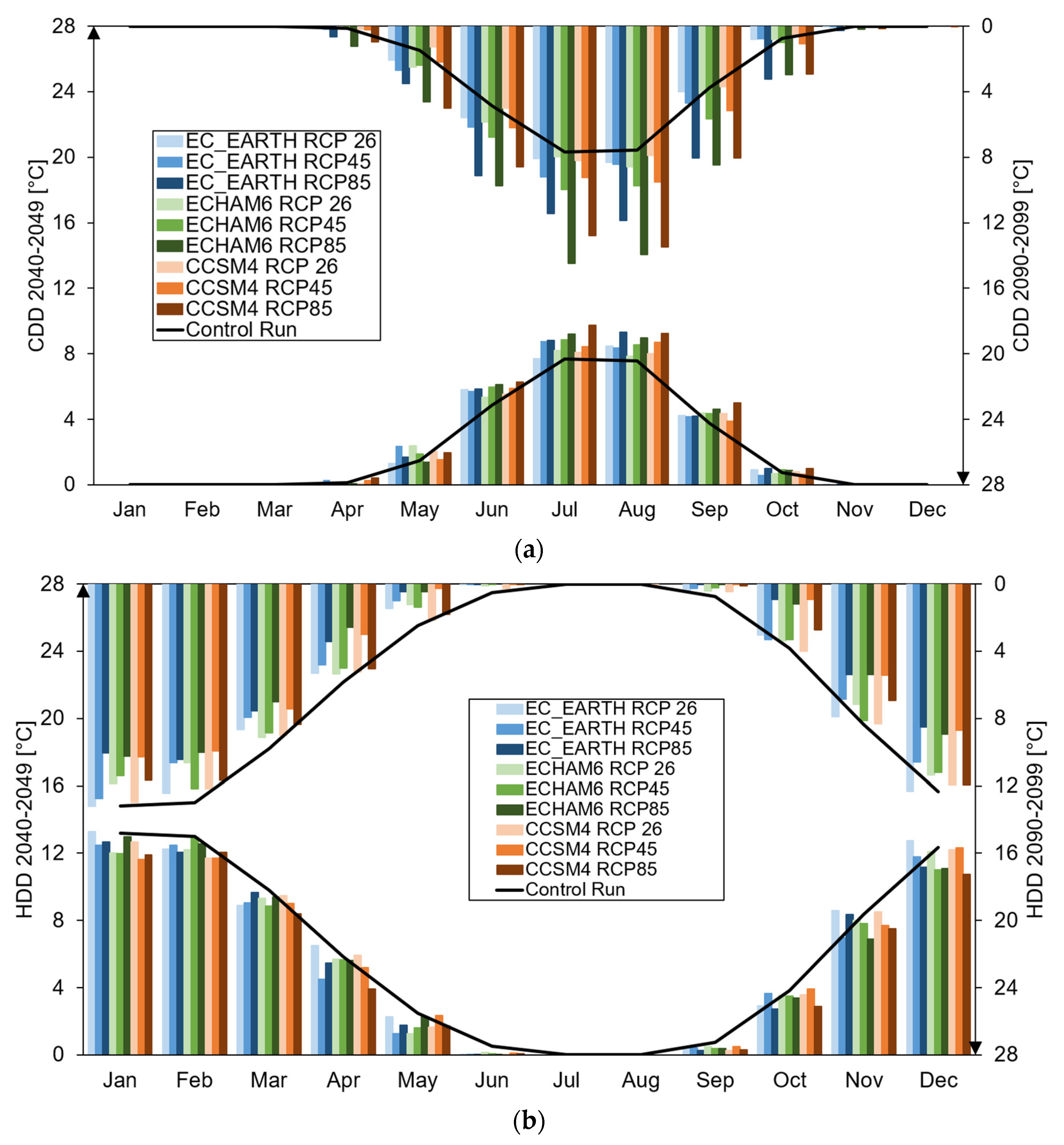
First, based upon the climate projections from our GCMs and RCPs, we studied the future values of HDD and CDD, reported in Figure 3.
In Figure 3a we display the average monthly CDD values during the half-century (2040–2049, hereon 2045), and during the end-of-century (2090–2099, hereon 2095), compared against the control run (CR) (2005–2013).
The two indices basically reflect the increase in the temperature as projected by the GCMs, in those periods when the temperature thresholds are exceeded. At the mid-century, a slight increase of CDD would occur, with largest changes in summer, June, July and August. The largest deviation from the control period reaches approx. +2 °C, given by CCSM4 under RCP8.5 in July. Outside of the summer period, however, no more than +1 °C is seen. At the end-of-century, different scenarios display large potential deviations, especially RCP8.5 scenarios, which exceed +3.5 °C between June and September, and with a maximum of +6.8 °C in July under ECHAM6, RCP8.5. The RCP4.5 scenarios never deviate by more than +2 °C, while RCP2.6 never exceeds +1 °C.
Figure 3b shows the average monthly HDD values at 2045, and at 2095 against CR. Considering the mid-century period, the change is less than −2 °C (i.e., there is less need of increasing temperatures for heating purposes), with peaks in April period for CCSM4, RCP8.5 with −1.9 °C. On the other hand, at 2095, CPR8.5 deviates between −2 ° C and −4 °C in fall and spring, with the other scenarios varying between −2 °C to 0 °C.
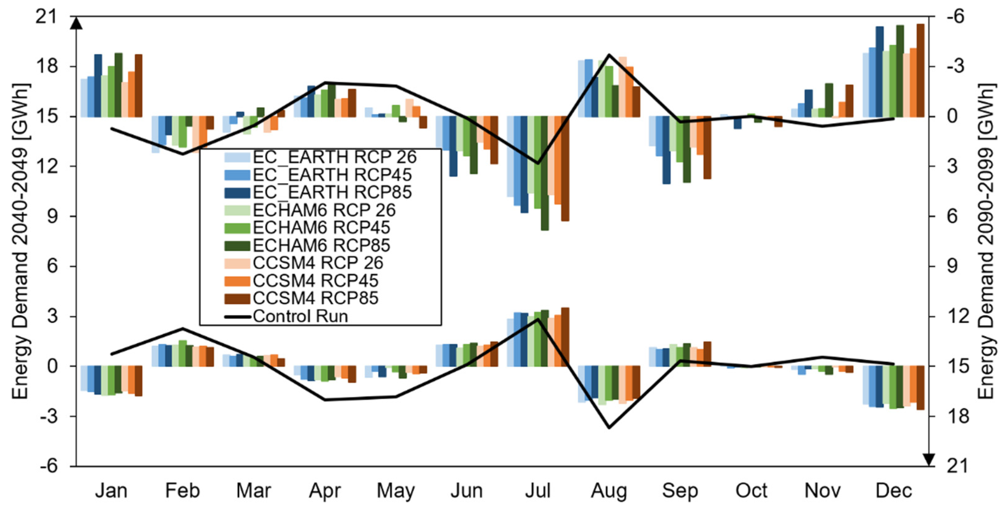
In Figure 4 we display the monthly variation in the demand for the two reference decades against CR. To offset the increase in energy demand forced by ever increasing GDP, we only report therein the variation of the climate-driven part.
Considering the monthly variations of energy demand, from the annual average value in mid-century compared to the control period, it can be seen that, as a result of the decrease in HDD values, a loss in energy demand occurs in the months of December and January, and this trend is more visible at the end of the century. Clearly, from Figure 4, we deduce that at 2045 and 2095, the largest increase in demand would be seen during spring to fall (June, July, and partly August when holidays largely decrease demand, September, and even October at 2095), as given by the larger need of energy for cooling. The largest increase is seen under RCP8.5 at 2095. Additionally, energy demand for heating decreases during December and January, especially at the end-of-century. At the yearly scale (not shown), little difference is seen in terms of energy demand.
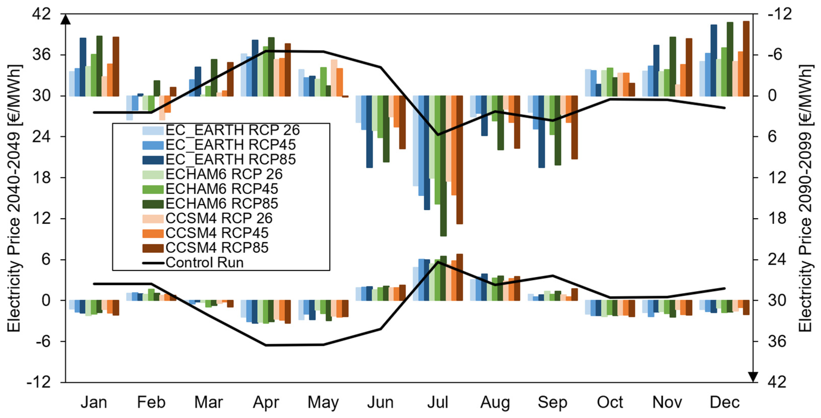
Figure 5 displays monthly averaged variations of the electricity price, again here offsetting the increase due to GDP.
The variation of energy demand reported above leads to a decreased price in winter and fall at 2045 and 2095 against CR. The spring period sees an increase at mid-century, with subsequent re-alignment at the historical price at 2095. At 2045, the energy price would increase during July and August, and even in September at 2095, again primarily under RCP8.5.

6. Discussion

6.1. Benchmark with Recent Literature

We could find some results in the available literature for benchmarking of our findings. In the Gridtech project reported above [28], the authors defined scenarios of future electric system’s behaviour until 2050, introducing a number of hypothesis concerning use of renewables. We compared our scenarios of annual load (TWh), and price until 2050 against the findings of the Gridtech project, to assess the capability of our simple model to represent future energy demand as set out using a more complex scheme.
In the EU project Highway2050 (2018) [19] the participants set out different scenarios (at 2050) for future schemes of the energy market, in terms of energy mix (solar, thermo, wind, nuclear, fossil, hydro) for production, also driving energy demand. Their five scenarios for energy demand could be used as a benchmark for our results.
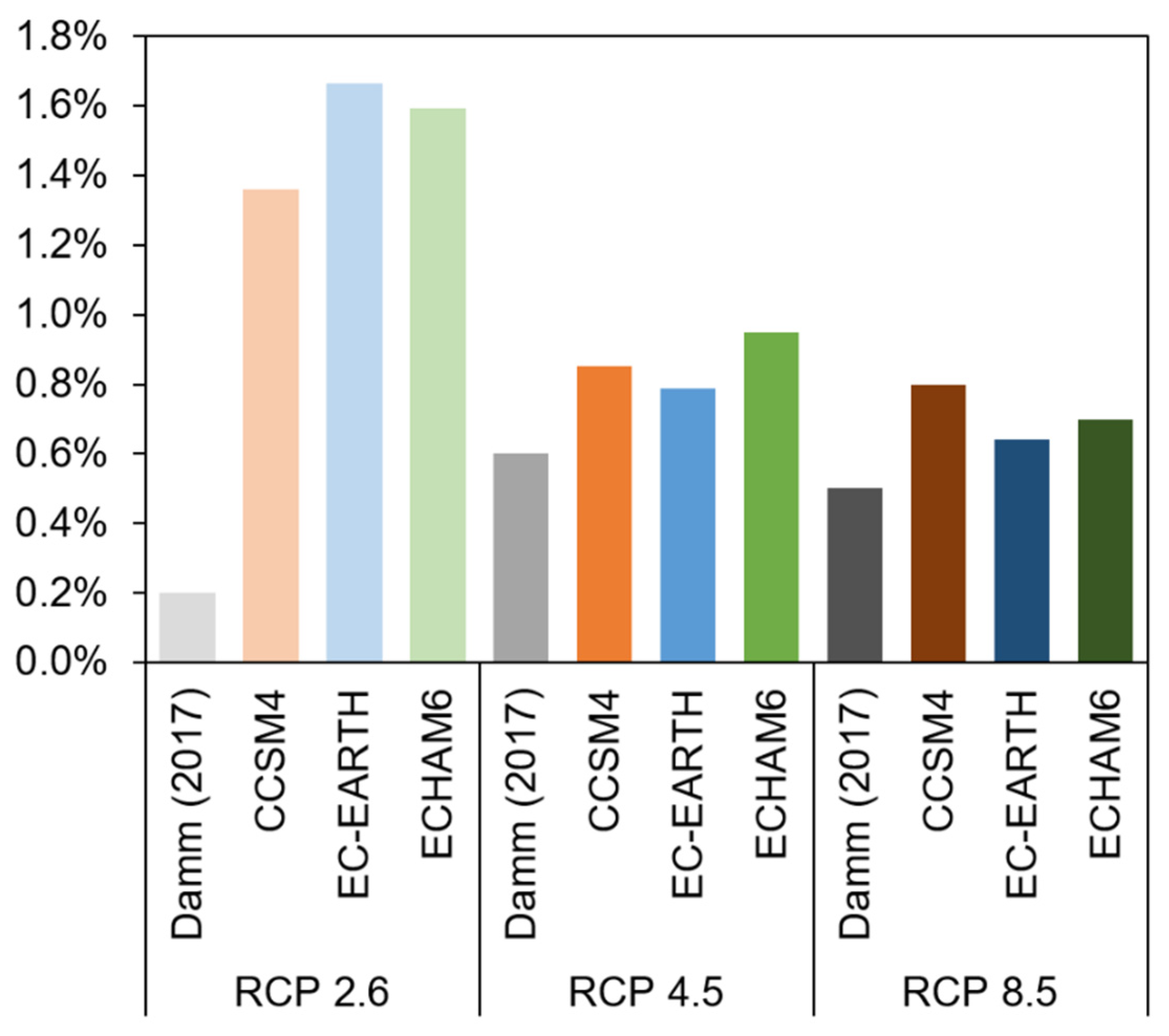
Damm et al. [29] built a temperature-driven model, to account for the impact on energy demand, given by an increase of temperature fixed at +2 °C within time windows of 30 years, centred on variable years, as depending on different RCPs (2071–2100 for RCP2.6, 2036–2065 for RCP4.5, 2006–2055 for RCP8.5). They used temperature data from five regional climate models (RCMs) from CMIP5, and provided averaged results for each RCP.
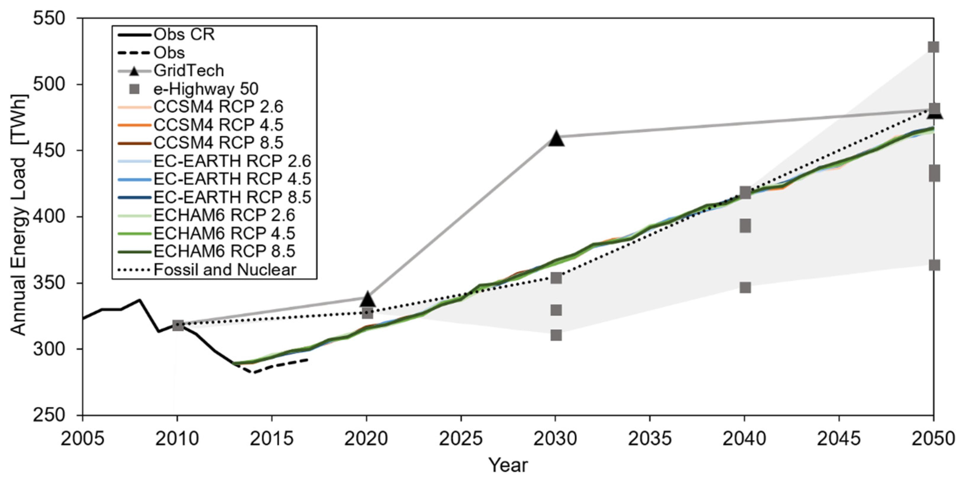
We could use these results to benchmark our climate-driven variation of demand under the same RCPs and periods. Figure 6 reports the annually observed load values in the CR period (2005–2013), plus the observed values during 2014–2017 (the latter years were not modelled in lack of meteorological data). Additionally, projected values until 2050 are reported for comparison, for the nine projected scenarios, somewhat overlapping, given the large contribution as given by the GDP term (that could not be extracted based on the available information from the two projects used for the benchmark).
Our model provides results that are somewhat consistent with those from the e-Highway2050 project until the half-century point (i.e., included within the boundaries of their five scenarios). The e-Highway2050 project and our model should have a largest correspondence in term of the scenario “Fossil and Nuclear”, highlighted in Figure 6. This scenario, as indicated by the name, considers an energy production system that is somewhat similar to the current one where, at the European level, large use of non-renewable sources and nuclear energy is pursued. Our model provides +3.2% at 2030 against the Fossil and Nuclear scenario, −0.5% in 2040, and −3.2% in 2050.
Conversely, the GridTech project displays annual loads comparable with our values near year 2020 (+6.9% against our model), with a subsequent large increase, much higher than our model (and e-Highway2050). Then, at the half-century point, GridTech converges (+3%). The Gridtech project considered different projections for the GDP until the half-century. Visibly, they assumed a larger increase than we did until 2040. However, it is not fully clear from their report how they projected GDP in the future. We used projections from the OEDC, which should be dependable enough for the present exercise.
A comparison of our results against Damm et al. [29] is given in Figure 7. We report therein the annual variation of the climate driven component of energy demand for our different scenarios, for the same periods as set out by the authors therein. Our model visibly diverges from theirs under RCP2.6, whereas it provides basically consistent changes under RCP4.5 and RCP8.5.
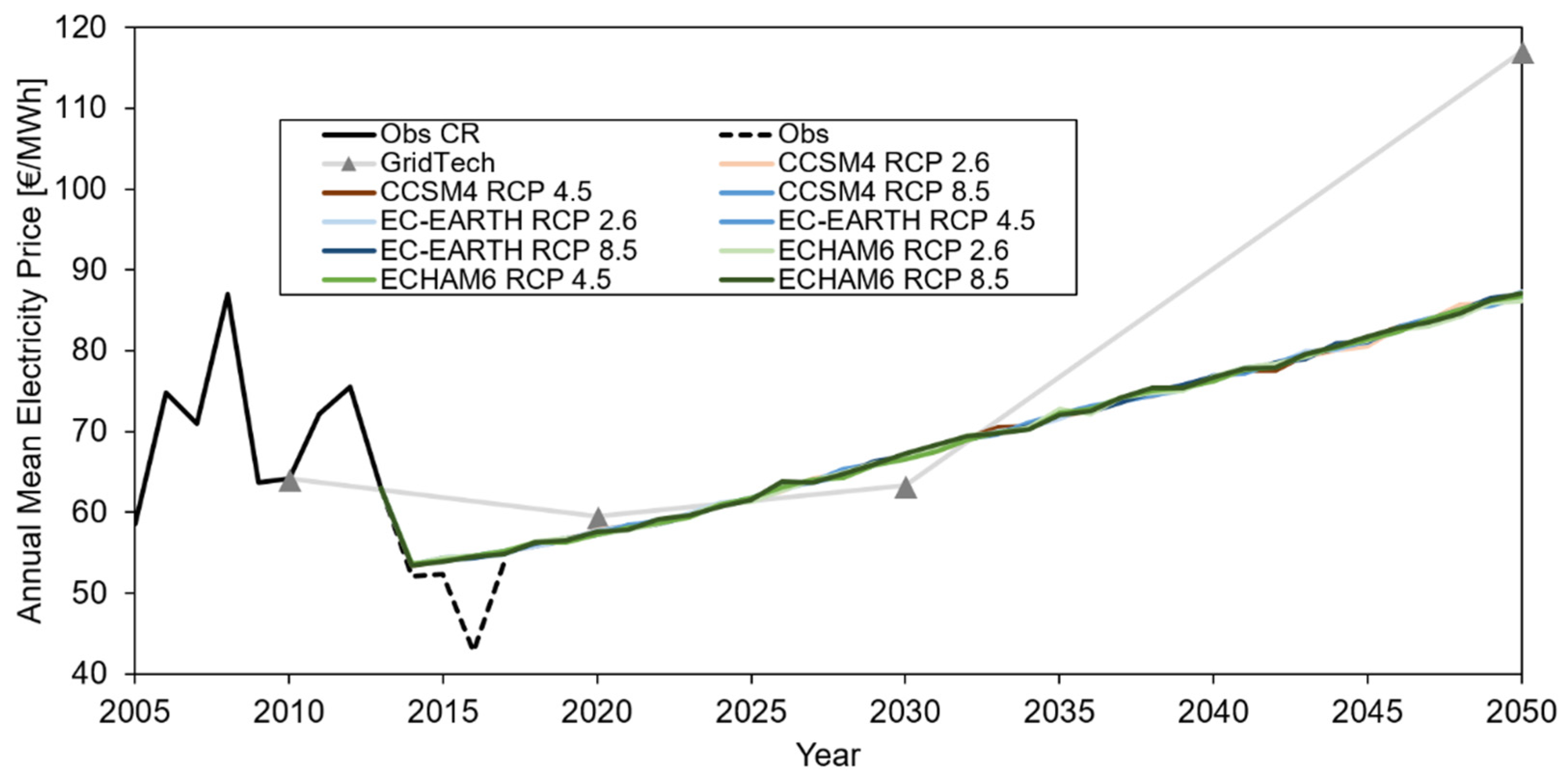
The electricity price model was benchmarked against the results of the GridTech project, the only one available for this purpose that we could find. Figure 8 shows the annually averaged energy price in the CR period (2005–2013), plus observed values during 2014–2017 (again not modelled due to a lack of meteorological data). Additionally, projected values until 2050 are reported for comparison, for the nine projected scenarios, again somewhat overlapping, given the large contribution as given by the GDP term.
Comparing with the GridTech project, our model provides similar values at 2020, and 2030 (+3.3% in 2020, and −5.9% in 2030, our model against GridTech). In 2050 our model delivers a much lower price instead (−25.7%). In our understanding, this results from the underlying assumption of GridTech, that no changes in the energy system would occur at 2050. Such assumption produces an increasing price, in response to the inability of the system to adapt to an increase in energy demand. Our model instead is able to react to an increase in demand, by increasing energy production (Equation (4)), and thus decreasing the final energy price consistently. In this sense, our model is slightly more consistent with the real-world behaviour of energy systems, being normally able to adjust the selling prices to increased demand over the long-term.

6.2. Hydropower Price and Production Assessment

The outputs of our methodology, namely present and future projected energy demand, and price, in response to climate, can be used as external drivers to force simulations of energy production from specific sectors for the purpose of testing the dependability and profitability of the sector themselves, under future climate changes.
The hydropower sector in Italy is a most critical one, as reported, and the proposed methodology can help develop credible projections of hydropower production in the future, as constrained by climate and hydrological conditions, demand and the market.
Indeed, expected climate change will affect, on the one hand, water availability and, on the other hand, energy demand and price [21] and, accordingly, one needs tools for proper hydropower regulation (i.e., reservoir management) under modified boundary conditions.
Among others, Ravazzani et al. [3] assessed the impacts of climate change on hydropower production of the largely regulated Toce river basin in the Italian Alps. They used simulations from two regional climate models to force Toce hydrology, and subsequently used a model of the hydropower system (SOdA, Simulatore ed Ottimizzatore di Aste idroelettriche, developed by the Company Enel Green Power-Energie Rinnovabili, of Italy), to define management rules under profit maximization constraints until 2050. They considered modified energy demand in response to temperature variations, but with a constant energy price in the future. Under such a hypothesis of constant energy prices, the changes of the hydrological regime expected during 2011–2050 would lead to significant changes in the reservoirs’ management policy, with anticipation of maximum storage, from August to July, and a drawdown of stored volume in August and September, to prepare for autumn inflows. At the half-century point, energy production would increase (+11%–+19%) in response to large precipitation increases until 2050 (+17%–+40%), with much uncertainty, however.
Gaudard et al. [4] studied the effect of modified hydropower production in Valais, Switzerland, under reduced streamflows in response to climate change. They showed that adequate management may mitigate losses. However, they would consider constant boundary conditions of price and demand. Gaudard et al. [30] further discussed potential changes of revenues of hydropower energy management throughout the century, highlighting large uncertainty in response to changes in prices.
Solaun et al. [31] analysed the effect climate change will have on the revenues and operations of hydroelectric power plants in a long-term frame. They found, in the absence of adaptive measures, that a decrease in the productivity is to be expected for the power plants they considered. However, they applied a methodological decision system that they define “ceteris paribus approach”, i.e., they considered many parameters constant in time, in particular, energy price.
Aili et al. ([32,33]) recently studied the hydropower system of the Mallero River, in the Northern Italian Alps. They used the hydrological model Poly-Hydro [1], fed with IPCC climate projections under three models and three RCPs, as here, and the SOdA production model (same as [3]), to project forward future streamflows, and subsequently evaluate future energy production. They foresaw a stream flow decrease at 2100 (from +1 to −25%, on average −7%), with the potential for increased flows during fall and winter, and a large decrease in summer, with subsequent decreased energy production at the half-century point (−2% similar for all scenarios), and end-of-century (−24%–+6%, −12% on average).
A preliminary investigation was pursued using our energy model here by Bombelli et al. [21,34]. They used Poly-Hydro to model and project forward hydrological fluxes in the complex Alta Valtellina valley hydropower system, based on IPCC climate projections under three models and three RCPs, as here. They included our energy price model within a hydropower management tool Poly-Power, able to mimic optimal hydropower management under given hydrological fluxes, and given demand/price conditions. They found that annual stream flows for hydropower production may decrease along the century (−21–+7%, on average −5% at the half-century; −17% to −2%, average −8%, at end-of-century). Energy production may be substantially constant under proper management (−9% to +15%, +3% on average) at the half-century, but at the end-of-century, under the warmest (and possibly most likely, see the Discussion in [21]) scenario RCP 8.5, a decrease of energy production would be consistently projected (−4% on average).
Stucchi et al. [35] coupled Poly-Hydro and Poly-Power to assess future energy production and revenues for the largely ice-fed Sabbione hydropower plant, at 2460 m asl in the Piemonte region of Italy. They projected largely modified future stream fluxes (−22% to −3%, −10% on average at the half-century, and −28% to −1%, average −13%, at the end-of-century), as due to reduced ice contribution, and uncertainly changing precipitation. Power production, driven by seasonal demand and water availability, would change (decrease) in the future (−27% to −8%, −15% on average at the half-century, and −32% to −5%, −16% on average at the end-of-century).
Accordingly, large uncertainty dwells into projections of scenarios of hydropower production throughout the 21st century, due to complex interaction between (i) the modified hydrological cycle in response to changing precipitation (with a large projected variability in positive/negative direction), temperature (ever increasing), and availability of ice melting in the glacierized areas (decreasing), (ii) energy demand (seasonally changing), and (iii) energy price (increasing on average, with large seasonal dependence), also under complex plants’ regulation.
The use of constant demand, and energy prices under future scenarios of water availability, may indeed reduce the credibility of future hydropower production scenarios.
Within such complex scenarios, the use of properly projected demand, and price conditions from our energy price models, may help in highlighting most realistic scenarios for reservoir management, and proper maximization until the end of the century.
The methodology proposed here is, therefore, likely to be useful, and will be exploited in the future to generate more dependable scenarios of hydropower production and, in general, of energy demand and price under expected climate change.

7. Conclusions

We introduced here a methodology to model the behaviour of energy demand and electricity price, and for projecting their trends under climate change, which we applied to the Italian electricity market. The method requires data of temperature, energy demand and electricity price in the region of interest, and can operate without a detailed knowledge of the internal system’s components. Its results are, however, comparable to other, more complex methods that take into account the main drivers of the energy system. The subsequent use of climate projections, e.g., from IPCC scenarios, as shown here, allows to build dependable projections under a what-if perspective.
Again, our projections reasonably match those from other more sophisticated methods. The method is general enough that it can be applied ideally to any energy system, provided proper data are available.
We developed the method with specific reference to application in the field of hydropower, most subject to climate change as reported [21,35], and we briefly reported examples of assessment of hydropower production under uncertain future climate change scenarios.
Present and prospective hydropower production depends upon an array of factors, including climate and hydrology, energy demand and price, and plants’ operation. Accordingly, proper assessment of modified energy demand/price, as displayed here, may improve the modelling chain for assessment of the hydropower potential, for management of present plants, and the design of future ones.
Notwithstanding the focus on hydropower here, our proposed approach can be virtually applied in several fields of energy production, whenever information of the present and future energy price, depending upon social and climate conditions, would be needed.
The method and results here, therefore, seem of great interest for policy-makers in the field of hydropower production (and energy, in general), for the study of future change in energy production demand, price and profitability.
Author Contributions

Conceptualization, G.M.B., A.B., D.B.; methodology, G.M.B.; software, G.M.B., A.S.; validation, G.M.B.; formal analysis, G.M.B.; investigation, G.M.B.; resources, A.B., D.B.; data curation, G.M.B.; writing-original draft preparation, G.M.B.; writing-review and editing, D.B.; visualization, G.M.B.; supervision, A.B., D.B.; project administration, D.B.

Funding

This research received no external funding.

Acknowledgments

The authors kindly acknowledge support to the presented research from Politecnico di Milano under the Project: Climate-Lab, an Interdepartmental Laboratory on Global Climate Change at Polimi.

Conflicts of Interest

The authors declare no conflict of interest.

References

  1. Akbari, H.; Soncini, A.; Dinpashoh, Y.; Fakheri-Fard, A.; Talatahari, S.; Bocchiola, D. Operation of two major reservoirs of Iran under IPCC scenarios during the 21ST Century. Hydrol. Process. 2018, 32, 3254–3271. [Google Scholar]
  2. D’Agata, C.; Soncini, A.; Bocchiola, D.; Maragno, D.; Smiraglia, C.; Diolaiuti, G. Recent area and volume loss of Alpine glaciers in the Adda River of Italy and their contribution to hydropower production. Cold Reg. Sci. Technol. 2018, 14, 172–184. [Google Scholar] [CrossRef]
  3. Ravazzani, G.; Valle, F.; Gaudard, L.; Mendlik, T.; Gobiet, A.; Mancini, M. Assessing Climate Impacts on Hydropower Production: The Case of the Toce River Basin. Climate 2016, 4, 16. [Google Scholar] [CrossRef]
  4. Gaudard, L.; Manfred, G.; Franco, R. Climate change impacts on hydropower management. Water Resour. Manag. 2013, 27, 5143–5156. [Google Scholar] [CrossRef]
  5. ACQWA Project. 2013. Available online: http://www.acqwa.ch/ (accessed on 15 October 2019).
  6. Bessec, M.; Fouquau, J. The non-linear link between electricity consumption and temperature in Europe: A threshold panel approach. Energy Econ. 2018, 30, 2705–2721. [Google Scholar] [CrossRef]
  7. TERNA. 2016. Available online: http://www.terna.it/ (accessed on 5 September 2019).
  8. Brunetti, M.; Maugeri, M.; Monti, F.; Nanni, T. Temperature and precipitation variability in Italy in the last two centuries from homogenized instrumental time series. Int. J. Climatol. 2006, 26, 345–381. [Google Scholar] [CrossRef]
  9. ISPRA. Valori Climatici Normali di Temperatura e Precipitazione in Italia nel 2017; Istituto Superiore per la Protezione e la Ricerca Ambientale ISPRA: Rome, Italy, 2018; p. 75, (In Italian). Available online: http http://www.isprambiente.gov.it/files2018/pubblicazioni/stato-ambiente/ (accessed on 15 October 2019).
  10. Weron, R. Electricity price forecasting: A review of the state-of-the-art with a look into the future. Int. J. Forecast. 2014, 30, 1030–1081. [Google Scholar] [CrossRef] [Green Version]
  11. Blanco-Novoa, Ó.; Fernández-Caramés, T.M.; Fraga-Lamas, P.; Castedo, L. An Electricity Price-Aware Open-Source Smart Socket for the Internet of Energy. Sensors 2017, 17, 643. [Google Scholar] [CrossRef]
  12. Guerci, E.; Rastegar, M.A.; Cincotti, S. Agent-based modelling and simulation of competitive wholesale electricity markets. In Handbook of Power Systems II. Energy Systems Book Series; Rebennack, S., Pardalos, P., Pereira, M., Iliadis, N., Eds.; Springer: Berlin/Heidelberg, Germany, 2011; pp. 241–286. [Google Scholar]
  13. Kanamura, T.; Ohashi, K. A Structural Model for Electricity Prices with Spikes-Measurement of Jump Risk and Optimal Policies for Hydropower Plant Operation. Energy Econ. 2007, 29, 1010–1032. [Google Scholar] [CrossRef]
  14. Keles, D.; Genoese, M.; Möst, D.; Fichtner, W. Comparison of extended mean-reversion and time series models for electricity spot price simulation considering negative prices. Energy Econ. 2012, 34, 1012–1032. [Google Scholar] [CrossRef]
  15. Swider, D.J.; Weber, C. Extended ARMA models for estimating price developments on day-ahead electricity markets. Electr. Power Syst. Res. 2007, 77, 583–593. [Google Scholar] [CrossRef]
  16. Gianfreda, A.; Grossi, L. Forecasting Italian electricity zonal prices with exogenous variables. Energy Econ. 2012, 34, 2228–2239. [Google Scholar] [CrossRef] [Green Version]
  17. Gareta, R.; Romeo, L.M.; Gil, A. Forecasting of electricity prices with neural networks. Energy Convers. Manag. 2006, 47, 1770–1778. [Google Scholar] [CrossRef]
  18. Siface, D.; Vespucci, M.; Gelmini, A. Development of the Stochastic Medium Term Market Simulation Model s-MTSIM. In Proceedings of the PMAPS 2012-12th International Conference on Probabilistic Methods Applied to Power Systems, Istanbul, Turkey, 10–14 June 2012. [Google Scholar]
  19. E-Highway2050 Project. 2018. Available online: http://www.e-highway2050.eu (accessed on 5 September 2019).
  20. Mima, S.; Criqui, P. The Costs of Climate Change for the European Energy System, an Assessment with the POLES Model. Environ. Model. Assess. 2015, 20, 303–319. [Google Scholar] [CrossRef] [Green Version]
  21. Bombelli, G.M.; Soncini, A.; Bianchi, A.; Bocchiola, D. Potentially modified hydropower production under climate change in the Italian Alps. Hydrol. Process. 2019, 33, 2355–2372. [Google Scholar] [CrossRef]
  22. Shourav, M.S.A.; Shahid, S.; Singh, B.; Mohsenipour, M.; Chung, E.S.; Wang, X.J. Potential Impact of Climate Change on Residential Energy Consumption in Dhaka City. Environ. Model. Assess. 2018, 23, 131–140. [Google Scholar] [CrossRef]
  23. Apadula, F.; Bassini, A.; Elli, A.; Scapin, S. Relationships between meteorological variables and monthly electricity demand. Appl. Energy 2012, 98, 346–356. [Google Scholar] [CrossRef]
  24. Isaac, M.; Van Vuuren, D. Modelling global residential sector energy use for heating and air conditioning in the context of climate change. Energy Policy 2009, 37, 507–521. [Google Scholar] [CrossRef]
  25. Scapin, S.; Apadula, F.; Brunetti, M.; Maugeri, M. High-resolution temperature fields to evaluate the response of Italian electricity demand to meteorological variables: An example of climate service for the energy sector. Theor. Appl. Climatol. 2015, 125, 729–742. [Google Scholar] [CrossRef]
  26. Groppelli, B.; Soncini, A.; Bocchiola, D.; Rosso, R. Evaluation of future hydrological cycle under climate change scenarios in a mesoscale Alpine watershed of Italy. Nat. Hazard. Earth Syst. 2011, 11, 1769–1785. [Google Scholar] [CrossRef] [Green Version]
  27. De Almeida, P.; Silva, P.D. Timing and future consequences of the peak of oil production. Futures 2011, 43, 1044–1055. [Google Scholar] [CrossRef]
  28. L’Abbate, A.; Calisti, R. Description of Four Scenarios for the Development of the European Electricity System up to 2050 (with Special Consideration of the Target Years 2020, 2030 and 2050) Incorporating New Innovative Technologies Fostering RES-Electricity and Storage Integration. GridTech Project, Deliverable D4.1 2015. Available online: http://www.gridtech.eu/ (accessed on 5 September 2019).
  29. Damm, A.; Köberl, J.; Prettenthaler, F.; Rogler, N.; Töglhofer, C. Impacts of +2 °C global warming on electricity demand in Europe. Clim. Serv. 2017, 7, 12–30. [Google Scholar] [CrossRef]
  30. Gaudard, L.; Gabbi, J.; Bauder, A.; Romerio, F. Long-term uncertainty of hydropower revenue due to climate change and electricity prices. Water Resour. Manag. 2016, 30, 1325–1343. [Google Scholar] [CrossRef]
  31. Solaun, K.; Cerdá, E. The Impact of Climate Change on the Generation of Hydroelectric Power—A Case Study in Southern Spain. Energies 2017, 10, 1343. [Google Scholar] [CrossRef]
  32. Aili, T.; Soncini, A.; Bianchi, A.; Diolaiuti, G.; Bocchiola, D. A method to study hydrology of high altitude catchments: The case study of the Mallero river, Italian Alps. Theor. Appl. Climatol. 2018. [Google Scholar] [CrossRef]
  33. Aili, T. Effetto del Cambiamenti Climatico Sulla Produzione Degli Impianti Idroelettrici a Serbatoio Della Valmalenco: Effect of Climate Change Upon Hydropower Production in the Reservoirs Plants of Valmalenco Valley. Master’s Thesis, Politecnico di Milano, Milan, Italy, 2017; p. 212. (In Italian). [Google Scholar]
  34. Bombelli, G.M. L’influenza del Cambiamento Climatico Sulla Produzione Idroelettrica dei Grandi Serbatoi Lombardi. Master’s Thesis, Politecnico di Milano, Milan, Italy, 2018. (In Italian). [Google Scholar]
  35. Stucchi, L.; Bombelli, G.M.; Bianchi, A.; Bocchiola, D. Hydropower potential of the Alpine cryosphere in the era of climate change: The case of a storage plant in Italy. Water 2019, 11, 1599. [Google Scholar] [CrossRef]
Figure 1. (a) Energy demand model calibration; on the x-axis the time period of calibration, on the y-axis the value of daily average energy demand observed and modelled. (b) Energy demand model validation; on the x-axis the time period of validation, on the y-axis the value of daily average energy demand observed and modelled.
Climate 07 00121 g001
Figure 2. (a) Price model calibration; on the x-axis the time period of calibration, on the y-axis the value of electricity price hourly observed and modelled. (b) Price model validation; on the x-axis the time period of calibration, on the y-axis the value of electricity price hourly observed and modelled.
Climate 07 00121 g002
Figure 3. (a) CDD monthly projections at mid-century period 2040–2049 (left y-axis) and end-of-century period 2090–2099 (right y-axis, values upside-down) against the control run period (2005–2013). (b) HDD monthly projections at the mid-century period 2040–2049 (left y-axis) and the end-of-century period 2090–2099 (right y-axis, values upside-down) against Control Run period (2005–2013).
Climate 07 00121 g003
Figure 4. Energy demand monthly projections, climate driven share, compared against the yearly mean, at the mid-century period 2040–2049 (left y-axis) and the end-of-century period 2090–2099 (right y-axis, values upside-down) against the control run period (2005–2013).
Climate 07 00121 g004
Figure 5. Electricity price monthly projections, climate driven share, compared with the yearly mean, in the mid-century period 2040–2049 (left y-axis) and end-of-century period 2090–2099 (right y-axis, values upside-down) against the control run period (2005–2013).
Climate 07 00121 g005
Figure 6. Annual load. Observed and projected values at 2050 for benchmarking against the results from GridTech and e-Highway 2050 projects.
Climate 07 00121 g006
Figure 7. Annual variation of the climate driven component of energy demand for our different scenarios. Benchmarking against Damm et al. [29], giving average values from 5 RCMs for each RCPs.
Climate 07 00121 g007
Figure 8. Electricity price. Observed and projected values to 2050 for benchmarking against the results from the GridTech project.
Climate 07 00121 g008
Table 1. Adaptation scores for calibration and validation of the Electricity Price Model and Energy Demand Model.
ModelCal/ValRMSER2R2log
Energy Demand ModelCalibration2.163GWh0.8670.873
Validation2.816GWh0.5830.623
Electricity Price ModelCalibration25.04€/MWh0.4990.593
Validation34.98€/MWh0.0630.173
Table 2. Model parameters.
Energy DemandElectricity Price-DailyElectricity Price-Hourly
ParameterValueParameterValueParameterValueParameterValue
α0.734Δ1.0 × 10⁻⁵γ1−0.175γ130.087
β0.041a02.536γ2−0.217γ140.067
γ0.059a100.037γ3−0.239γ150.076
φ0.501a11−0.001γ4−0.248γ160.081
σ0.010 η 1.210γ5−0.246γ170.093
δ1−0.350a−0.003γ6−0.221γ180.109
δ2−0.450b0.400γ7−0.147γ190.115
δ3−0.500σ0.401γ8−0.026γ200.119
δ4−0.200 γ90.078γ210.099
δ50.300 γ100.123γ220.055
γ110.132γ23−0.022
γ120.129γ24−0.104