Abstract
The long-term temporal trends and spatial distribution of Ozone (O3) over Egypt is presented using monthly data from both the Atmospheric Infrared Sounder (AIRS) and the model Modern-Era Retrospective analysis for Research and Applications (MERRA) datasets. The twelve-year monthly record (2005–2016) of the Total Ozone Column (TOC) has a spatial resolution of 1 × 1° from AIRS and 0.5 × 0.625° from the MERRA-2 dataset. The average monthly, seasonal and interannual time series are analyzed for their temporal trends, while the seasonal average spatial distributions are compared. It was found that MERRA-2 underestimated AIRS measurements. Both AIRS and MERRA-2 have their minimum monthly averages of TOC in February 2013. The maximum monthly average TOC from AIRS is 321.48 DU in July 2012, while that from MERRA-2 is 303.48 in April 2011.
1. Introduction
Ozone is a major greenhouse gas, thus, it plays an important role in both weather and climate, and its impact varies from global to regional scales [1,2]. While it represents only 0.0012% of the atmospheric composition [3], ozone acts as an absorber for the energetic particle from the solar ultraviolet radiation (UV), protecting the earth from harmful radiation [4,5], which has a harmful effect on human health particularly on the skin [6,7]. The observed increase in UV radiation at the earth’s surface has been due to the decrease of amount of ozone at the stratospheric atmospheric layer [8,9,10], which is caused by photochemical losses related to anthropogenic reasons [11,12,13,14].
Therefore, the spatial and temporal variation of O3 over global and regional domains has become an important research subject [14]. Global total column ozone concentration (which is referred to as ozone in the stratosphere) decreased a few percent between the 1970s and the start of this century [15]. In the stratosphere, ozone plays the role of a natural and beneficial screen in relation to the harmful effects of ultraviolet for the organic matter. In the troposphere, ozone is a secondary pollutant that is produced during the atmospheric photo-oxidation of volatile organic compounds under the presence of nitrogen oxides emitted, mainly, by anthropogenic activities, while surface ozone is considered to be the most damaging air pollutant in terms of adverse effects on human health, vegetation, crops and materials in Europe and may become worse in the future [16,17,18,19,20]. The total amount of ozone at any location on the globe is defined as the summation of all the ozone in the atmosphere directly above that location [21]. Evaluation of ozone profile and variability from different satellite data against in situ measurements (on board the NSF/NCAR Gulfstream-V aircraft during the Stratosphere-Troposphere Analyses of Regional Transport in 2008 (START08) experiment) from Atmospheric Infrared Sounder (AIRS), Infrared Atmospheric Sounding Interferometer (IASI), and the Ozone Monitoring Instrument (OMI) shows that the three satellite products have an acceptable capability to represent the variability of ozone in the upper troposphere and lower stratosphere. Statistical analyses revealed that the three satellite products captured 80% of the variability of ozone monitored in the aircraft data [22]. The comparison between the measured and reanalysis of Total Ozone Column (TOC) over Cairo city between 1979 and 2014 shows good agreement with (r = 0.91) the correlation coefficient [23]. The highest ozone measurements were recorded in the summer of 2007 over Cairo city [23]. The long-term variability of ozone from the main four ground urban observation stations in Cairo, Aswan, Matrouh and Hurgada shows that negative trend values in ozone are the dominant features during the period 1990–2014 at all stations [24]. Formation of Ozone over the greater Cairo was investigated based on two measurement campaigns. The first one was in 1990 and lasted for 3 weeks based on measurements from three different sites (Shoubra El-Kheima, Mokattam Hills and Helwan). The second one was in 1991 and lasted for 7 months from April to October based on one site at El-Kobba. It was found that ozone is produced over the industrial sites at north and center of Cairo and transported southward by the northerly winds [25]. Also, high average ozone levels were observed during the night in the spring and the summer [25]. The automatic station located 30 km south of Dekhla Oasis in Egypt in the Lybian desert (powered by a photovoltaic generator system to measure the vertical ozone flux) confirmed that high ozone fractions were recorded when northerly winds prevailed [26].
There is an interest in investigating the impact of air pollutants on agricultural crops, and this interest has focused on the long-term low-level effects of the main phytotoxic gases on crop production [27,28,29,30,31,32]. Periodic exposure to air pollutants may cause yield losses [27,33,34,35,36,37,38,39]. Apart from crop yield losses, changes in plant development and reduction in net growth can occur [40,41,42], as well as changes in crop quality [43,44,45,46]. Ozone is the main phytotoxic air pollutant in the Mediterranean area [47,48,49,50,51,52,53,54]. The high levels of O3 over Egypt can cause significant decrease in the growth and the local varieties of crop plants [45]. On testing and selecting multiple sensitive and environmentally successful Egyptian bioindicator plants for ozone (O3), four plant species (jute, clover, garden rocket and alfalfa) were found to be more sensitive to O3 than the universally used O3-bioindicator, tobacco Bel W3 [55].
The objective of the current work is to highlight the analysis of spatial-temporal of TOC over Egypt (23.7–36.2° N and 21.5–32.3° E), which could help understanding how Egypt contributes in this issue. In this study, TOC from the remote sensor AIRS and MERRA-2 datasets is used to generate the long-term trend and the spatial distribution over Egypt; a comparison between both sources of TOC is established. As far as the author is aware, research of this kind has not been conducted over Egypt before.
2. Methodology
In this study, TOC data from two different sources is introduced. Those sources are: AIRS and the model Modern-Era Retrospective analysis for Research and Applications version 2 (MERRA-2) dataset.
2.1. AIRS Sensor
AIRS was launched into orbit in 2002 aboard NASA’s Aqua satellite; its primary goal is to support weather and climate research [56]. An innovative atmospheric sounding group of visible, infrared, and microwave sensors constitute the multispectral range of AIRS. The Level-3 data from AIRS (Daytime/Ascending) is used with a 1 × 1° spatial resolution monthly gridded retrieval product (AIRX3STM) version (v006) [57].
AIRS has previously demonstrated its capacity to capture TOC. AIRS/Aqua level-3 daily gridded products (AIRX3STD) 1 × 1° spatial resolution (version 5) data could successfully detect O3 from large forest fires [58]. Benchmarking of AIRS (version 5)-retrieved ozone profiles with TOC has already been done by the World Ozone and Ultraviolet Radiation Data Center. The biases from the collected ozonesonde (O3SND) were less than 5% for both stratosphere and troposphere [22].
2.2. MERRA-2 Model Data
The MERRA-2 [59] dataset consists of worldwide meteorological variables hosted by NASA and generated by the Goddard Space Flight Center. This dataset is generated by the Goddard Earth Observing System Model, version 5 (GEOS-5). The spatial resolution is 0.625° in latitude and 0.5° in longitude (approx. 50 km). It replaces the original MERRA reanalysis [60]. Daily TOC and relative humidity (RH) from AIRS on NASA’s Aqua satellite are used to identify the presence of SI over Rocky Mountain National Park in observational data, and to validate MERRA-2 reanalysis of TOC, since AIRS data are not assimilated by MERRA-2. AIRS is equipped to measure both meteorological variables and chemical profiles [61,62,63].
The MERRA-2 dataset is monthly averaged [64]. Since 2004, MERRA-2 has assimilated satellite retrievals of TOC from the Ozone Monitoring Instrument [33,65] and stratospheric O3 profiles from the Microwave Limb Sounder [66,67,68]. TOC from the MERRA-2 dataset in the lower stratosphere has good representation and has proven the agreement with ozonesondes [69,70]. MERRA-2’s total ozone agrees with Total Ozone Mapping Spectrometer (TOMS) data (1980–1993) very well, with less than 2% bias and less than 6% difference in standard deviation, which is close to the assumed observation error of 5% [70]. There is a good representation of the variability of stratospheric ozone in MERRA-2. The difference in standard deviations between the reanalysis data and the independent limb satellite data range from 11% for SAGE II in the lower stratosphere to less than 5% at 4.3 hPa [70].
3. Results
The temporal trends of TOC, which include monthly average, seasonal and interannual time series, are introduced in Section 3.1. The spatial distribution seasonal maps are presented in Section 3.2. Both time series and spatial maps of TOC are in Dobson units (DU).
3.1. Temporal Trend
Tropospheric ozone ground observations show that ozone has increased globally during the 20th century. Ozone records over Europe show that ozone has doubled between the 1950s and 2000 [71]. Daily total ozone observations from TOMS over Dundee city in Scotland in the period (1979–1992) show a significant negative trend [72]. Aircrafts measured significant upper tropospheric trends in one or more seasons above multiple locations the North Atlantic Ocean, the north-eastern USA, the Middle East, Europe, northern India, southern Japan and China. From 1990 to 2010, surface ozone trends have varied according to the region. Western Europe showed increasing ozone in the 1990s followed by a decrease since 2000 [71]. In eastern US, surface ozone has decreased strongly in the summer, remained unchanged in the spring, and it has increased in the winter; in other locations such as the in western US, ozone has increased the most in the spring. Surface ozone in East Asia is increasing [71]. In general, MERRA-2 underestimates TOC compared to AIRS over Egypt. Monthly average of TOC—in DU—over 12 years (2005–2016) is introduced in Figure 1 for both AIRS and MERRA-2. From AIRS, average TOC was 294.5 ± 16.5 DU. The max TOC was 321.14 DU on 1 July 2012 (286.2 DU from MERRA-2), while the minimum was 253.89 DU in February 2013. On the other hand, from MERRA-2, the average TOC was 277.8 ± 11.934 DU. The max TOC was 303.478 DU in April 2011 (317.01 DU from AIRS), while the minimum was 248.655 DU in February 2013. The basic statistics are summarized in Table 1.
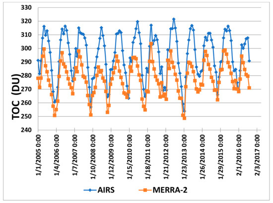
Figure 1.
Temporal evolution of monthly average total ozone column over Egypt for the period (2005–2016) from AIRS and MERRA-2.

Table 1.
Basic descriptive statistics for monthly average total ozone column over Egypt for the period (2005–2016) from AIRS and MERRA-2.
Figure 2 shows the probability density function (PDF) of TOC over Egypt of the 11-year dataset for both AIRS and MERRA-2, along with four tested distributions. Errors of fitting for the tested PDF using Kolmogorov–Smirnov goodness of fit are given in Table 2. The best fit between the given distribution and the hypothesized continuous distributions has the lowest error value. The best fit is ordered, and the order is shown in the parentheses. For AIRS, it is shown that that Weibull distribution has the best goodness of fit, with 0.08744 between the four tested distributions. Regarding the normal distribution case, the best goodness of fit, with 0.0473, was for the MERRA-2 data.
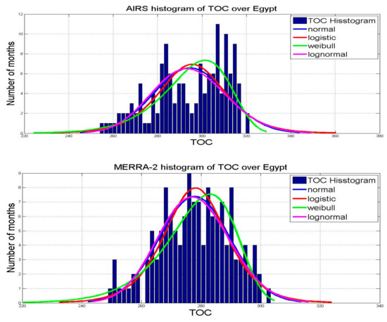
Figure 2.
TOC histogram over Egypt for 12 years from AIRS (upper) and MERRA-2 (lower).
Table 2.
Goodness of fit for both AIRS and MERRA-2 data over Egypt.
Interannual monthly regional average time series (2006–2016) of TOC—in DU—over Egypt from both AIRS and MERRA-2 are shown in Figure 3. For AIRS, it is shown that July had the highest TOC values, while December had the lowest. It is noticeable from both AIRS and MERRA-2 that February had negative slope between 2010 and 2013, with an increase starting from 2014. February 2013 had the lowest TOC concentration in the eleven-year period of shown data with no clear reason behind this bottom point until now. On the other hand, for the MERRA-2 dataset, it can be seen that October 2011 had the highest TOC values, while February 2013 had the lowest. The basic statistics (maximum, minimum, average, variance and standard deviation) for interannual monthly average TOC from both AIRS and MERRA-2 are summarized in Table 3 and Table 4. The corresponding year for max and min monthly average TOC is represented between the parentheses.
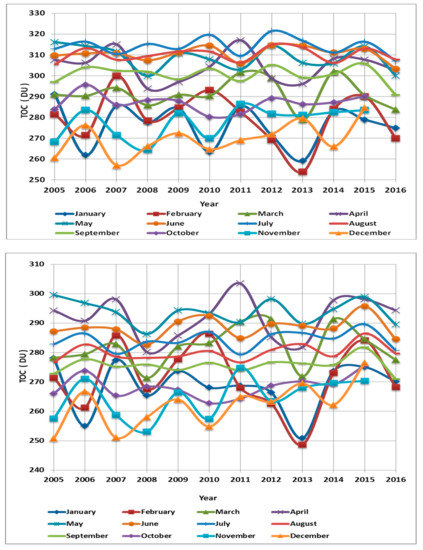
Figure 3.
Interannual monthly average time series of TOC in Dobson Units (DU) over Egypt for the period (2005–2016) from AIRS (upper) and MERRA-2 (lower).
Table 3.
Interannual monthly regional average statistics TOC for 12 years from AIRS. Numbers in parentheses represent the corresponding year.
Table 4.
Interannual monthly regional average statistics TOC for 12 years from MERRA-2. Numbers in parentheses represent the corresponding year.
Seasonal average time series for TOC—in DU—is highlighted in Figure 4. It is shown that TOC in the summer (JJA) has the highest values, followed by the spring, then the fall season. The winter (DJF) has the lowest TOC. The highest TOC concentration in the summer, especially June, is comparable with previous studies conducted over Cairo by Y. Aboel Fetouh in 2013 [23]. The statistics of the seasonal average time series for TOC are introduced in Table 5. The number between the parentheses corresponds to each maximum or minimum seasonal TOC over Egypt.
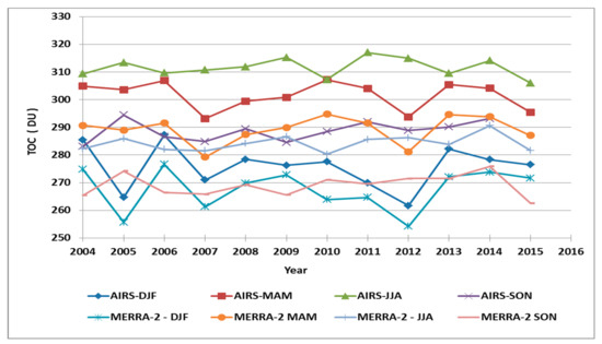
Figure 4.
Seasonal monthly average time series of TOC in Dobson Unit (DU) over Egypt (2005–2016) from AIRS and MERRA-2.
Table 5.
Seasonal average time series statistics of TOC for 12 years from both AIRS and MERRA-2. The numbers in the parentheses represent the corresponding year.
As shown in Table 5, both AIRS and MERRA-2 sensors recorded maximum and minimum TOC measurements in the same years, 2006 and 2012, which occurred in the DJF season; however, this behavior is not repeated in any of the remaining seasons (MAM, JJA or SON), as shown by the table, i.e., the two sensors’ maximum and minimum TOC measurements do not overlap in the same year again. AIRS provides the maximum TOC measurement for the DJF season with a value of 287.227 DU in year 2006, while the minimum was 261.67 DU in year 2012. On the other hand, MERRA-2 shows that the max. TOC in the DJF season was 276.644 DU and the minimum was 254.259 DU. Figure 5 shows the boxplots for the different seasons from both AIRS and MERRA-2. For AIRS, it is shown that the highest average season is JJA and the lowest is DJF, while for MERRA-2 the highest average season is MAM and the lowest is SON.
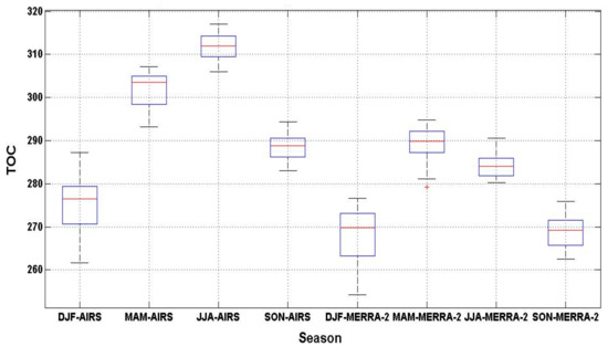
Figure 5.
Boxplot seasonal monthly average of TOC (2005–2016) from AIRS and MERRA-2.
The Mann-Kendall (MK) [73,74,75] test is a way to identify if a monotonic upward (increase) or downward (decrease) trend exists for a specific variable over time. This test is run on the seasonal monthly average TOC in Figure 4. The results of Mann-Kendall test for all seasonal monthly average TOCs for both AIRS and MIRRA-2 data found that there was no trend. Table 6 summarizes the analysis of the eight seasonal average time series from both AIRS and MERRA-2 under the Mann-Kendall test. There was no significant trend (p > 0.05) in the time series.
Table 6.
Summary of the results of Mann-Kendall test for the eight seasonal monthly average TOCs over Egypt (2005–2016).
3.2. Spatial Distribution
The spatial distribution of seasonal monthly averages of TOC over the 12-year study period for both AIRS and MERRA-2 is shown in Figure 6. The spatial maps show that MERRA-2 also underestimates TOC over Egypt. Once again, for AIRS, the winter map (DJF) reveals the lowest spatial distribution, while the summer map (JJA) reveals the highest spatial distribution, confirming the time series in Figure 3.
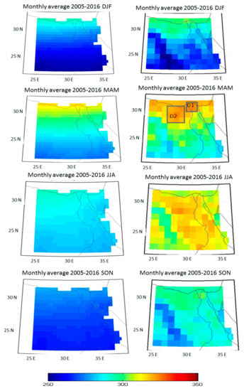
Figure 6.
Seasonal average of TOC in (DU) over Egypt for winter (DJF), spring (MAM), summer(JJA) and fall (SON), for the period (2005–2016). Two domains, D1 and D2, are shown for further analysis on MAM map for MERRA-2 (left panel) and AIRS (right panel).
The right panel from Figure 6 shows also that the north coast of Egypt has the highest TOC in the spring (higher than the summer), which is associated with the main and secondary Mediterranean cyclones [24], while the higher concentration in summer is due to trans-boundary transportation of ozone from Europe [23,76]. Those regions include the Nile Delta (D1) and the Qattara Depression and area (D2). Anthropogenic activities and emissions in urban and industrial areas have had an impact on ozone production and concentration [77]. The Nile Delta (D1) region has high levels of anthropogenic activities. Meanwhile, Qattara Depression is considered an active dust source and contains both clay and sand. In addition, several studies have suggested a link between ozone and fine particulate matter (PM) concentrations [76,77,78,79]. This may be the reason for high ozone in the D2 domain. On the other hand, the left panel from Figure 6 shows that MERRA-2 does not have the capability to capture the same variability of TOC over Egypt as AIRS does, although it has higher resolution.
4. Conclusions and Future Works
The AIRS and MERRA-2 datasets provide observations for the TOC that allow the tracking and monitoring of its concentration and its temporal and spatial variability over Egypt. Monthly and seasonal average time series show that summer months feature the highest TOC. Comparing the two sensors with regard to TOC measurement, it was found that the spatial maps from AIRS over Egypt can identify the location of high and low concentrations of ozone, while spatial maps from MERRA-2 underestimate TOC and do not have the capability to capture the same variability shown by AIRS. It was concluded that the MERRA-2 dataset also underestimates the temporal TOC over Egypt in comparison to the AIRS data set. The statistical quantities for the 12-year temporal trend over Egypt are summarized.
Future work shall include investigation of the construction of TOC from numerical models, such as numerical weather research and forecasting models coupled with chemistry (WRF-chem). The sensitivity of TOC to different chemical mechanisms should be investigated. In addition to a study on the correlation between TOC from AIRS and aerosol optical depth from (MODIS and numerical weather research and forecasting coupled with chemistry (WRF-chem) model) shall be established.
Conflicts of Interest
The author declares no conflict of interest.
References
- Kiehl, J.T.; Schneider, T.L.; Portmann, R.W.; Solomon, S. Climate forcing due to tropospheric and stratospheric ozone. J. Geophys. Res. 1999, 104, 31239–31254. [Google Scholar] [CrossRef]
- Rex, M.; von der Salawitch, R.J.P.; Gathen, N.R.; Harris, P.; Chipperfield, M.; Naujokat, B. Arctic ozone loss and climate change. Geophys. Res. Lett. 2004, 31, L04116. [Google Scholar] [CrossRef]
- Kerr, J.B.; McElroy, C.T. Total ozone measurements made with the Brewer ozone spectrophotometer during STOIC. J. Geophys. Res. 1989, 100, 9225–9230. [Google Scholar] [CrossRef]
- Varotsos, C.A.; Chronpoulos, G.J.; Katsiki, S.; Sakellariou, N.K. Further evidence of the role of air-pollution on solar ultraviolet-radiation reaching the ground. Int. J. Remote Sens. 1995, 16, 1883–1886. [Google Scholar] [CrossRef]
- Alexandris, D.; Varotsos, C.; Kondratyev, K.Y.; Chronopoulos, G. On the altitude dependence of solar effective UV. Phys. Chem. Earth Part C Sol. Terr. Planet. Sci. 1999, 24, 515–517. [Google Scholar] [CrossRef]
- World Health Organization (WHO). Protection Against Exposure to Ultraviolet Radiation; Technical Report WHO/EHG #17; WHO: Geneva, Switzerland, 1995. [Google Scholar]
- Kondratyev, K.Y.; Varotsos, C.A. Global total ozone dynamics—Impact on surface solar ultraviolet radiation variability and ecosystems. Environ. Sci. Pollut. Res. 1996, 3, 205. [Google Scholar] [CrossRef] [PubMed]
- Fioletov, V.E.; McArthur, L.; Kerr, J.E.; Wardle, D.I. Long-term variations of UV-Birradiance over Canada estimated from Brewer observations and derived from ozone and pyranometer measurements. J. Geophys. Res. 2001, 106, 2307–2309. [Google Scholar] [CrossRef]
- Frederick, J.E.; Manner, V.W.; Booth, C.R. Inter-annual variability in solar ultraviolet irradiance over decadal time scales at latitude 55 south. Photochem. Photobiol. 2001, 74, 771–779. [Google Scholar] [CrossRef]
- Molina, M.J.; Rowland, F.S. Stratospheric sink for chlorofluoromethanes: Chlorine atom-catalysed destruction of ozone. Nature 1974, 249, 810–812. [Google Scholar] [CrossRef]
- Farman, J.C.; Gardiner, B.G.; Shanklin, J.D. Large losses of total ozone in Antarctica reveal seasonal ClOx/NOx interaction. Nature 1985, 315, 207–210. [Google Scholar] [CrossRef]
- Stolarski, R.S.; Krueger, A.J.; Schoeberl, M.R.; McPeters, R.D.; Newman, P.A.; Alpert, J.C. Nimbus 7 satellite measurements of the springtime Antarctic ozone decrease. Nature 1986, 322, 808–811. [Google Scholar] [CrossRef]
- Harris, N.R.P.; Ancellet, J.; Bishop, L.; Hofmann, D.J.; Kerr, J.B.; McPeters, R.D.; Prendez, W.J.; Randel, J.; Staehelin, B.H.; Subbaraya, A. Trends in stratospheric and free tropospheric ozone. J. Geophys. Res. 1997, 102, 1571–1590. [Google Scholar] [CrossRef]
- World Meteorological Organization (WMO). Scientific Assessment of Ozone Depletion: Global Ozone Research and Monitoring Project; Technical Report 50; WMO: Geneva, Switzerland, 2006. [Google Scholar]
- World Meteorological Organization (WMO). Scientific Assessment of Ozone Depletion: Global Ozone Research and Monitoring Project; Report No. 52; WMO: Geneva, Switzerland, 2011. [Google Scholar]
- Ochoa-Hueso, R.; Munzi, S.; Alonso, R.; Arróniz-Crespo, M.; Avila, A.; Bermejo, V.; Bobbink, R.; Branquinho, C.; Concostrina-Zubiri, L.; Cruz, C. Ecological Impacts of Atmospheric Pollution and Interactions with Climate Change in Terrestrial Ecosystems of the Mediterranean Basin: Current Research and Future Directions. Environ. Pollut. 2017, 227, 194–206. [Google Scholar] [CrossRef] [PubMed]
- Paoletti, E.; de Marco, A.; Beddows, D.C.S.; Harrison, R.M.; Manning, W.J. Ozone levels in European and USA cities are increasing more than at rural sites, while peak values are decreasing. Environ. Pollut. 2014, 192, 295–299. [Google Scholar] [CrossRef] [PubMed]
- Proietti, C.; Anav, A.; de Marco, A.; Sicard, P.; Vitalea, M. A multi-sites analysis on the ozone effects on Gross Primary Production of European forests. Sci. Total Environ. 2016, 556, 1–11. [Google Scholar] [CrossRef] [PubMed]
- Sicard, P.; Alessandro, A.; Alessandra, D.; Elena, P. Projected global tropospheric ozone impacts on vegetation under different emission and climate scenarios. Atmos. Chem. Phys. Discuss. 2017, 1–34. [Google Scholar] [CrossRef]
- Lefohn, A.S.; Malley, C.S.; Smith, L.; Wells, B.; Hazucha, M.; Simon, H.; Naik, V.; Mills, G.; Schultz, M.G.; Paoletti, E.; et al. Tropospheric Ozone Assessment Report: Global ozone metrics for climate change, human health, and crop/ecosystem research. Elem. Sci. Anth. 2018, 6, 28. [Google Scholar] [CrossRef]
- David, W.F.; Michaela, I. Twenty Questions and Answers about the Ozone Layer. 2014. Available online: http://www.atmos.umd.edu/~rjs/class/spr2017/readings/WMO_Ozone_2010_QAs.pdf (accessed on 29 May 2018).
- Pittman, J.V.; Pan, L.L.; Wei, J.C.; Irion, F.W.; Liu, X.; Maddy, E.S.; Barnet, C.D.; Chance, K.; Gao, R.-S. Evaluation of AIRS, IASI, and OMI ozone profile retrievals in the extratropical tropopause region using in situ aircraft measurements. J. Geophys. Res. 2009, 114, D24109. [Google Scholar] [CrossRef]
- Fetouh, Y.A.; El Askary, H.; El Raey, M.; Allali, M.; Sprigg, W.A.; Kafatos, M. Annual Patterns of Atmospheric Pollutions and Episodes over Cairo Egypt. Adv. Meteorol. 2013, 2013, 984853. [Google Scholar] [CrossRef]
- Badawy, A.; Basset, H.A.; Eid, M. Spatial and Temporal Variations of Total Column Ozone over Egypt. J. Earth Atmos. Sci. 2017, 2, 1–16. [Google Scholar]
- Güsten, H.; Heinrich, G.; Weppner, J.; Abdel-Aal, M.M.; Abdel-Hay, F.A.; Ramadan, A.B.; Tawfik, F.S.; Ahmed, D.M.; Hassan, G.K.Y.; Cvitašd, T.; et al. Ozone formation in the greater Cairo area. Sci. Total Environ. 1994, 155, 285–295. [Google Scholar] [CrossRef]
- Güsten, H.; Heinrich, G.; Monnich, D.; Sprung, D.; Weppner, J.; BakrRamadan, A.; El-Din, M.R.M.E.; Ahmed, D.M.; Hassan, G.K.Y. On-line measurements of ozone surface fluxes: Part II; surface-level ozone fluxes onto the Sahara desert. Atmos. Environ. 1996, 30, 911–918. [Google Scholar] [CrossRef]
- Weigel, H.J.; Adaros, G.; Jäger, H.J. An open top chamber study with filtered and non-filtered air to evaluate effects of air pollutants on crops. Environ. Pollut. 1987, 47, 231–244. [Google Scholar] [CrossRef]
- De Temmerman, L.; Vandermeiren, K.; Guns, M. Effects of air filtration on spring wheat grown in open-top chambers at a rural site. I. Effect on growth, yield and dry matter portioning. Environ. Pollut. 1992, 77, 1–5. [Google Scholar] [CrossRef]
- Schenone, G.; Botteschi, G.; Fumagali, I.; Montinaro, F. Effects of ambient air pollution in opentop chambers on bean (Phaseolus vulgaris L.) I. Effects on growth and yield. New Phytol. 1992, 122, 689–697. [Google Scholar] [CrossRef]
- Schenone, G.; Fumagali, I.; Mignanego, L.; Montinaro, F.; Soldatini, G.F. Effects of ambient air pollution in open-top chambers on bean (Phaseolus vulgaris L.). II. Effects on photosynthesis and stomatal conductance. New Phytol. 1994, 126, 309–331. [Google Scholar] [CrossRef]
- Hassan, I.A. Physiological and biochemical response of potato (Solanum tuberosum L. Cv. Kara) to O3 and antioxidant chemicals: Possible roles of antioxidant enzymes. Ann. Appl. Biol. 2006, 146, 134–142. [Google Scholar] [CrossRef]
- Hassan, I.A. Interactive effects of O3 and CO2 on growth, physiology of potato (Solanum tuberosum L.). World J. Environ. Sustain. Dev. 2010, 7, 1–12. [Google Scholar]
- Heagle, A.S.; Philbeck, R.B.; Rogers, H.H.; Letchworth, M.B. Dispersing and monitoring O3 in open-top field chambers for plant-effects studies. Phytopathology 1979, 69, 15–20. [Google Scholar] [CrossRef]
- Pande, P.C.; Mansfield, T.A. Responses of spring barely to SO2 and NO2 pollution. Environ. Pollut. 1985, 38, 87–97. [Google Scholar] [CrossRef]
- Schenone, G.; Lorenzini, G. Effects of regional air pollution on crops in Italy. Agric. Ecosyst. Environ. 1992, 38, 55–66. [Google Scholar] [CrossRef]
- Ali, E.A. Damage to plants due to industrial pollution and their use as bioindicators in Egypt. Environ. Pollut. 1993, 81, 251–255. [Google Scholar] [CrossRef]
- Dizengremel, P.; Le Thiec, D.; Bagard, M.; Jolivet, Y. Ozone risk assessment for plants: Central role of metabolism-dependent changes in reducing power. Environ. Pollut. 2008, 156, 11–15. [Google Scholar] [CrossRef] [PubMed]
- Dizengremel, P.; Le Thiec, D.; Hasenfratz-Sauderm, M.P.; Vaultier, M.N.; Bagard, M.; Jolivet, Y. Metabolic-dependent changes in plant cell redox power after ozone exposure. Plant Biol. 2009, 11, 35–42. [Google Scholar] [CrossRef] [PubMed]
- Dizengremel, P.; Vaultier, M.N.; Le Thiec, D.; Cabane, M.; Bagard, M.; Gerant, D.; Joëlle, G.; Allah Dghim, A.; Richet, N.; Afif, D.; et al. Phosphoenolpyruvate is at the crossroads of leaf metabolic responses to ozone stress. New Phytol. 2012, 195, 512–517. [Google Scholar] [CrossRef] [PubMed]
- Gould, R.P.; Mansfield, T.A. Effects of SO2 and NO2 on growth and translocation in winter wheat. J. Exp. Bot. 1988, 39, 389–399. [Google Scholar] [CrossRef]
- Hassan, I.A. Interactive effects of salinity and ozone pollution on photosynthesis, stomatal conductance, growth, and assimilate partitioning of wheat (Triticum aestivum L.). Photosynthetica 2004, 42, 111–118. [Google Scholar] [CrossRef]
- Hatata, M.; Badr, R.; Ibrahim, M.; Hassan, I.A. Effects of O3 and CO2 on growth, yield and physiology of wheat (Triticum aestivum L.). Curr. World Environ. 2013, 8, 421–429. [Google Scholar]
- Peleijel, H.; Skärby, L.; Wallin, G.; Sellden, G. Effects of grain quality of spring wheat exposed to O3 in OTCs. In The European Communities on Open-Top Chambers, Results on Agricultural Crops 1987–1988; Air Pollution Rept.; Bonte, J., Mathy, P., Eds.; CEC: Brussels, Belgium, 1989; pp. 73–89. [Google Scholar]
- Fuhrer, J.; Lehnherr, B.; Tschannen, W.; Moeri, P.B.; Shariat-Madari, H. Effects of O3 on the grain composition of spring wheat grown in open-top field chambers. Environ. Pollut. 1990, 65, 181–192. [Google Scholar] [CrossRef]
- Vandermeiren, K.; De Temmerman, L.; Staquet, A.; Baeten, H. Effects of air filtration on spring wheat grown in open-top field chambers at a rural site. II. Effects on mineral portioning, sulphur and nitrogen metabolism and on grain quality. Environ. Pollut. 1992, 77, 7–14. [Google Scholar] [CrossRef]
- Hassan, I.A. Air pollution in Alexandria region, Egypt. II: Effect of regional air pollution on growth and yield of bean (Phaseolus vulgaris L. cv. Giza 6). In Proceedings of the 6th Egyptian Botanical Conference, Cairo, Egypt, 24–26 November 1998; Volume 3, pp. 469–479. [Google Scholar]
- Lorenzini, G.; Nali, C.; Panicucci, A. Surface ozone in Pisa (Italy): A six-year study. Atmos. Environ. 1994, 28, 3155–3164. [Google Scholar] [CrossRef]
- Hassan, I.A. Air pollution in Alexandria region, Egypt. I. An investigation of air quality. Int. J. Environ. Educ. Inf. 1999, 18, 67–78. [Google Scholar]
- Hassan, I.A.; Ashmore, M.R.; Bell, J.N.B. Effects of O3 on the stomatal behaviour of Egyptian verities of radish (Raphanus sativus L. cv. Baladey) and turnip (Brassica rapa L. cv. Sultani). New Phytol. 1994, 128, 243–249. [Google Scholar] [CrossRef]
- Hassan, I.A.; Ashmore, M.R.; Bell, J.N.B. Effect of ozone on radish and turnip under Egyptian field conditions. Environ. Pollut. 1995, 89, 107–114. [Google Scholar] [CrossRef]
- Hassan, I.A.; Basahi, J.M.; Ismail, I.; Habbebullah, T. Spatial distribution and temporal variation in ambient ozone and its associated NOx in the atmosphere of Jeddah City. Saudi Arab. Aerosol. Air Qual. 2013, 13, 1712–1722. [Google Scholar] [CrossRef]
- Velissariou, D.; Gimeno, B.S.; Badiani, M.; Fumagalli, I.; Davison, A.W. Records of O3 visible injury in the ECE Mediterranean region. In Critical Levels for Ozone in Europe: Testing and Finalizing the Concept; UN-ECE Workshop Report; Kärelampi, L., Skärby, L., Eds.; University of Kuopio: Kuopio, Finland, 1996; pp. 343–350. [Google Scholar]
- Gimeno, B.S.; Bermejo, V.; Reinert, R.A.; Zheng, Y.; Barnes, J.D. Adverse effects of ambient ozone on watermelon yield and physiology at a rural site in Eastern Spain. New Phytol. 1999, 144, 245–260. [Google Scholar] [CrossRef]
- Pellegrini, E.; Carucci, M.G.; Campanella, A.; Lorenzini, G.; Nali, C. Ozone stress in Melissa officinalis plants assessed by photosynthetic function. Environ. Exp. Bot. 2011, 73, 94–101. [Google Scholar] [CrossRef]
- Madkour, S.A.; Laurence, J.A. Egyptian plant species as new ozone indicators. Environ. Pollut. 2002, 120, 339–353. [Google Scholar] [CrossRef]
- AIRS/AMSU/HSB Version 6 Data Release User Guide, Jet Propulsion Laboratory; Version 1.2.1.; California Institute of Technology: Pasadena, CA, USA, 2005.
- AIRS Science Team/Joao TexeiraAIRS/Aqua L3 Monthly Standard Physical Retrieval (AIRS+AMSU) 1 Degree × 1 Degree V006; Goddard Earth Sciences Data and Information Services Center (GES DISC): Greenbelt, MD, USA, 2013. [CrossRef]
- Rajab, J.M.; MatJafri, M.Z.; Lim, H.S.; Abdullah, K. Daily distribution Map of Ozone (O3) from AIRS over Southeast Asia. Energy Res. J. 2010, 2, 158–164. [Google Scholar] [CrossRef]
- Bosilovich, M.; Akella, S.; Coy, L.; Cullather, R.; Draper, C.; Gelaro, R.; Kovach, R.; Liu, Q.; Molod, A.; Norris, P.; et al. MERRA-2: Initial Evaluation of the Climate; NASA/TM–2015–104606; National Aeronautics and Space Administration (NASA): Greenbelt, MD, USA, 2015; Volume 43, p. 139. [Google Scholar]
- Rienecker, M.M.; Suarez, M.J.; Gelaro, R.; Todling, R.; Bacmeister, J.; Liu, E.; Bosilovich, M.G.; Schubert, S.D.; Takacs, L.; Kim, G. MERRA—NASA’s Modern-Era Retrospective Analysis for Research and Applications. J. Clim. 2011, 24, 3624–3648. [Google Scholar] [CrossRef]
- Susskind, J.; Barnet, C.; Blaisdell, J.; Iredell, L.; Keita, F.; Kouvaris, L.; Molnar, G.; Chahine, M. Accuracy of geophysical parameters derived from Atmospheric Infrared Sounder/Advanced Microwave Sounding Unit as a function of fractional cloud cover. J. Geophys. Res. 2006, 111, D09S17. [Google Scholar] [CrossRef]
- Chahine, M.T.; Pagano, T.S.; Aumann, H.H.; Atlas, R.; Barnet, C.; Blaisdell, J.; Chen, L.; Divakarla, M.; Fetzer, E.J.; Zhou, L.; et al. AIRS: Improving weather forecasting and providing new data on greenhouse gases. Bull. Am. Meteorol. Soc. 2006, 87, 911–926. [Google Scholar] [CrossRef]
- Aumann, H.H.; Chahine, M.T.; Gautier, C.; Goldberg, M.D.; Kalnay, E.; McMillin, L.M.; Revercomb, H.; Rosenkranz, P.W.; Smith, W.L.; Susskind, J.; et al. AIRS/AMSU/HSB on the aqua mission: Design, science objectives, data products, and processing systems. IEEE Trans. Geosci. Remote Sens. 2003, 41, 253–264. [Google Scholar] [CrossRef]
- Bosilovich, M.G.; Lucchesi, R.; Suarez, M. MERRA-2: File Specification GMAO Office Note No. 9 (Version 1.1). 2016. Available online: http://gmao.gsfc.nasa.gov/pubs/docs/Bosilovich785.pdf (accessed on 20 June 2016).
- Levelt, P.F.; van den Oord, G.H.J.; Dobber, M.R.; Malkki, A.; Visser, H.; de Vries, J.; Stammes, P.; Lundell, J.O.V.; Saari, H. The Ozone Monitoring Instrument. IEEE Trans. Geosci. Remote Sens. 2006, 44, 1093–1101. [Google Scholar] [CrossRef]
- Waters, J.W.; Froidevaux, L.; Harwood, R.S.; Jarnot, R.F.; Pickett, H.M.; Read, W.G.; Siegel, P.H.; Cofield, R.E.; Filipiak, M.J.; Walch, M.J.; et al. The Earth Observing System Microwave Limb Sounder (EOS MLS) on the Aura satellite. IEEE Trans. Geosci. Remote Sens. 2006, 44, 1075–1092. [Google Scholar] [CrossRef]
- Gelaro, R.; McCarty, W.; Suarez, M.J.; Todling, R.; Molod, A.; Takacs, L.; Bosilovich, M.G.; Schubert, S.D.; Takacs, L.; Zhao, B.; et al. The Modern-Era Retrospective Analysis for Research and Applications, Version 2 (MERRA-2). J. Clim. 2017, 30, 5419–5454. [Google Scholar] [CrossRef]
- McCarty, W.; Coy, L.; Gelaro, R.; Huang, A.; Merkova, D.; Smith, E.; Meta, S.; Wargan, K. MERRA-2 Input Observations: Summary and Assessment; NASA/TM–2016–104606; NASA: Greenbelt, MD, USA, 2016; Volume 46, p. 64. [Google Scholar]
- Wargan, K.; Labow, G.; Frith, S.; Pawson, S.; Livesey, N.; Partyka, G. Evaluation of the ozone fields in NASA’s MERRA-2 reanalysis. J. Clim. 2017, 30, 2961–2988. [Google Scholar] [CrossRef] [PubMed]
- Wargan, K.; Pawson, S.; Olsen, M.A.; Witte, J.C.; Douglass, A.R.; Ziemke, J.R.; Strahan, S.E.; Nielsen, J.E. The global structure of uppertroposphere-lower stratosphere ozone in GEOS-5: A multiyear assimilation of EOS Aura data. J. Geophys. Res. Atmos. 2015, 120, 2013–2036. [Google Scholar] [CrossRef]
- Cooper, O.R.; Parrish, D.D.; Ziemke, J.; Balashov, N.V.; Cupeiro, M.; Galbally, I.E.; Gilge, S.; Horowitz, L.; Jensen, N.R.; Lamarque, J.-F.; et al. Global distribution and trends of tropospheric ozone: An observation-based review. Elem. Sci. Anth. 2014, 2, 29. [Google Scholar] [CrossRef]
- Cracknell, A.P.; Varotsos, C.A. Ozone depletion over Scotland as derived from Nimbus-7 TOMS measurements. Int. J. Remote Sens. 1994, 15, 2659–2668. [Google Scholar] [CrossRef]
- Gilbert, R.O. Statistical Methods for Environmental Pollution Monitoring; Wiley: Hoboken, NJ, USA, 1987. [Google Scholar]
- Mann, H.B. Non-parametric tests against trend. Econometrica 1945, 13, 163–171. [Google Scholar] [CrossRef]
- Kendall, M.G. Rank Correlation Methods, 4th ed.; Charles Griffin: London, UK, 1975. [Google Scholar]
- Duncan, B.N.; West, J.J.; Yoshida, Y.; Fiore, A.M.; Ziemke, J.R. The influence of European pollution on ozone in the Near East and northern Africa. Atmos. Chem. Phys. 2008, 8, 2267–2283. [Google Scholar] [CrossRef]
- Berntsen, T.K.; Isaksen, I.S.A.; Myhre, G.; Fuglestvedt, J.S.; Stordal, F.; Larsen, T.A.; Freckleton, R.S. Shine Effects of anthropogenic emissions on tropospheric ozone and its radiative forcing. J. Geophys. Res. 1997, 102, 28101–28126. [Google Scholar] [CrossRef]
- Schwartz, J. Air pollution and hospital admissions for respiratory disease. Epidemiology 1996, 7, 20–28. [Google Scholar] [CrossRef] [PubMed]
- Dockery, D.W.; Pope, C.A.; Xu, X.P.; Spengler, J.D.; Ware, J.H.; Fay, M.E.; Ferris, B.G.; Speizer, F. An association between air-pollution and mortality in 6 United States cities. N. Engl. J. Med. 1993, 329, 1753–1759. [Google Scholar] [CrossRef] [PubMed]
© 2018 by the author. Licensee MDPI, Basel, Switzerland. This article is an open access article distributed under the terms and conditions of the Creative Commons Attribution (CC BY) license (http://creativecommons.org/licenses/by/4.0/).