Abstract
The Madden Julian Oscillation (MJO) is the largest contributor to intraseasonal weather variations in the tropics. It is associated with a broad region of enhanced rainfall that moves slowly eastward over the Indian and western Pacific Oceans, which has global impacts on atmospheric circulations. A number of recent observational and modeling studies have suggested that the MJO is becoming stronger as the oceans warm. In this study, the author explores the sensitivity of the MJO to ocean warming in a recently developed Lagrangian Atmospheric Model (LAM), which has been shown to simulate robust and realistic MJOs in previous work. Numerical simulations suggest that ocean warming leads to more frequent and intense MJOs that propagate more rapidly and cover a larger region of the tropics. The strengthening of the MJO is attributed to enhanced surface fluxes of moisture coming from the warmer ocean waters. While the LAM simulations have a number of limitations owing to idealized physical parameterizations and the use of prescribed sea surface temperatures, they provide additional evidence that the MJO will strengthen if the oceans continue to warm, and they also shed light on the mechanism of this strengthening.
1. Introduction
The Madden Julian Oscillation (MJO) is a large-scale equatorial convective disturbance that moves slowly eastward over the warmest waters of the Indian and West Pacific Oceans [1,2]. It has a typical period of 45–50 days [3] and a propagation speed of about 5 m/s [4]. It has global impacts on weather and climate, affecting monsoons over multiple continents [5,6], the frequency and intensity of tropical cyclones [7,8], and the timing and duration of El Ninos [9,10].
There is growing evidence that the MJO is becoming more frequent and intense with time as the oceans warm. Slingo et al. [11] used zonally integrated equatorial zonal wind as a metric of MJO activity, and noted a substantial increase in the late 1970s, which seemed to be associated with a warming in the Indian Ocean. Jones and Carvalho [12] examined changes in the MJO starting in 1958, and found positive trends in lower- and upper-level zonal wind anomalies and the number of summer and winter MJO events, some of which were statistically significant at the 5% confidence level. Jones et al. [13] developed a stochastic model that predicts an increasing number of MJO events due to increasing sea surface temperatures (SSTs) under the A1B global warming scenario. Takahashi et al. [14] examined changes in the MJO in 12 coupled climate models, and found that 7 of 12 predicted intensification over time, with a tendency for El Nino-like SST warming in these models. Arnold et al. [15] analyzed the MJO in a coupled climate model that used embedded cloud resolving models to simulate atmospheric convection [16]. They found that MJO variance nearly doubled between a control run and run, with the number of events increasing by 20–30 percent. A steeper vertical gradient in moisture—a direct result of warming oceans—led to the MJO intensification. Carlson and Caballero [17] noted enhanced MJO-like activity in aquaplanet simulations with increasing concentrations, which led to equatorial superrotation. Song and Seo [18] compared MJO activity in 19th and 20th century coupled climate simulations, and they found a 33 percent increase in MJO amplitude between the centuries, which they attributed to increasing sea surface temperatures (SSTs) in the central and eastern Pacific. Adames et al. [19] noted that the MJO intensifies with increasing carbon dioxide concentrations in simulations conducted with an atmospheric general circulation model coupled to a mixed layer ocean model.
In this study the author uses a recently developed Lagrangian atmospheric model (LAM) to study how the MJO responds to increases in SSTs. Numerical simulations suggest that, with all other factors held fixed, a uniform ocean warming leads to more frequent and more intense MJOs that cover a larger region of the tropics. Model diagnostics suggest that the MJO strengthens in response to increases in surface fluxes of moisture that are ultimately a consequence of the non-linear nature of the Clausius–Clapeyron equation.
This paper is organized as follows. Section 2 describes the LAM, the experimental design, and the method used to construct composites of the MJO. Section 3 compares simulations of the MJO under the current climate to those under a climate with with warmer oceans. Section 4 discusses the results in light of related studies. Section 5 presents the conclusions.
2. Materials and Methods
The main source of data for this study is simulations of the global atmosphere conducted with a recently developed Lagrangian atmospheric model (LAM) [20,21,22,23]. This section describes the model, how the simulations were configured, and the methods used to analyze the data.
2.1. Lagrangian Atmospheric Model
The LAM simulates atmospheric motions by predicting the movements of individual parcels of air [20]. It uses prescribed SSTs, a simple land surface model, and idealized radiative and cloud microphysics schemes [22,23]. One unique feature of the model is its convective parameterization, which moves parcels vertically in response to convective instability [22,24]. Although the LAM is probably best described as a model of intermediate complexity [25], it does have variable surface elevations, and it generates rainfall patterns that are competitive with CMIP5 models [26] in terms of fidelity to observations [23]. Moreover, our previous work [21,22,23,24] established that the LAM simulates more realistic MJOs than those in a typical CMIP5 model [27], which is one reason why the author elected to use the LAM to study how the MJO will change as the oceans warm.
The version of the LAM used in this study has the following improvements to that used by Haertel et al. [23]. First, the radiation scheme is now applied on a regular (as opposed to Lagrangian) vertical grid, with low and high optical depth components tuned on this grid independently, and a simple representation of cloud radiative effects. Second, The land surface model now has spatially variable albedos. Third, the LAM now has a prognostic ice variable allowing for the explicit calculation of melting and freezing contributions to atmospheric heating. After these changes were implemented, model parameters were tuned to obtain a robust MJO (e.g., Figure 1). Since the new model’s basic state (e.g., zonal wind and precipitation patterns) is not substantially different from that presented in [23], it is not discussed it in this paper.
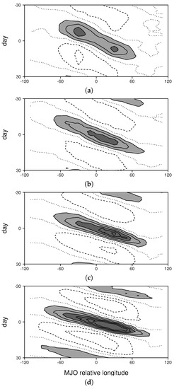
Figure 1.
Composite time/longitude series of rainfall for: (a) the observed MJO; (b) the control run; (c) the 3 K warming experiment; and (d) the 7 K warming experiment. The contour interval is 1 mm/day with values greater than 1 (3) mm/day shaded light (dark) gray.
2.2. Model Configuration and Experiments
The general approach in this paper is to compare simulations forced with recently observed SST patterns (for 1998–2009) to those in which the observed SSTs are increased by a uniform amount (dT). Each simulation is spun up for 90 days using the mean January 1998 SST as a basis for the SST forcing, and then run with observed SSTs for 1998–2009 increased by the increment dT. Land conditions are predicted using a simple, single-layer land surface model that calculates shortwave heating, longwave cooling, and moisture storage and evaporation [22,23]. The equivalent Eulerian model resolution of the LAM is about 3.75/1.875 degrees longitude/latitude, with 34 vertical levels. Model runs are conducted for dT = 0, 1, 3, 5, and 7 K. This paper focuses on the questions of how and why the MJO changes as the oceans warm. It is important to recognize that these simulations are a sensitivity test of how the LAM MJO changes with uniform ocean warming, and not a prediction of MJO changes under a global warming scenario. The latter is much more involved, requiring ocean coupling and carefully changing radiation to reflect anthropogenic influences. Therefore, the reader is cautioned that multiple processes are excluded that have the potential to affect MJO amplitude, such as ocean/atmosphere coupling, structural changes in SST patterns, and changes to atmospheric radiation unrelated to water vapor. Nevertheless, the LAM simulations exhibit the same kinds of changes to the MJO as do more realistic climate change experiments [15,18] and, owing to their more idealized nature, the LAM simulations are easier to interpret.
2.3. Composite MJOs
For each simulation, composite MJOs are constructed using the method of Haertel et al. [24]. Large-scale, eastward-propagating rainfall anomalies are tracked over the equatorial Indian and West Pacific Oceans, and their vertical and horizontal structures are constructed for initiating, mature, and dissipating stages of the MJO using rawinsonde data. All data are placed in the longitudinal frame of reference of the convective anomaly, so longitude 0 lies as the center of the region of heaviest rainfall (but latitude represents distance from the equator). This method of compositing MJOs is used for the following reasons: (1) the analysis is constructed in the frame of reference of the MJO’s convective anomaly, which is a key for understanding the relationship between convection and surface fluxes, and the sensitivity of the MJO to ocean warming in particular; (2) this is a compositing method that the author developed, so using it provides continuity with prior research; and (3) the resulting composite MJO, which is used to evaluate the modeled MJO, is based entirely on sounding data with no component coming from a model forecast. The observational composite MJO is based on 44 MJO events that occurred between 1996 and 2009, with sounding data coming from the Integrated Global Radiosonde Archive [28] and rainfall data from the Global Precipitation Climatology Project [29]. For more details on the method, the reader is referred to [24].
To estimate the impact of perturbations to surface fluxes on low-level humidity in the composite MJO, the author simulated surface moistening for a hypothetical collection of air parcels that were advected by the low-level flow. To keep calculations simple, the flow was averaged for the layer 700–1000 hPa, so that the parcels were essentially representing columns of air in the lower troposphere. Parcels were tracked for a five-day period, and cumulative changes in their humidity resulting from surface flux perturbations were computed. Changes in precipitable water that would result from low-level advection and surface flux perturbations alone were then calculated. This method isolated the impacts of two particular physical processes to assess their potential role in causing the MJO to change as the oceans warm.
3. Results
3.1. The Composite MJO in the Control Run
When the LAM is run using unaltered, observed SSTs as a forcing, it generates an MJO with a comparable amplitude, rate of propagation, and zonal extent to those observed in nature (Figure 1a,b). It also reproduces much of the observed vertical and horizontal structures of MJO zonal wind and moisture perturbations (Figure 2a,b, Figure 3a,b, and Figure 4a,b). Since the the LAM’s success at simulating the MJO has been discussed in several previous studies [21,22,23,24], these results are not elaborated on here, but instead are presented so that they may be compared to the ocean warming experiments discussed below.

Figure 2.
Composite vertical structure of zonal wind for the mature stage of the MJO for: (a) the observed MJO; (b) the control run; (c) the 3 K warming experiment; and (d) the 7 K warming experiment. The contour interval is 0.5 m/s, and values greater (less) than 0.5 (−0.5) m/s are shaded dark (light) gray.
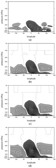
Figure 3.
Composite vertical structure of specific humidity for the mature stage of the MJO for: (a) the observed MJO; (b) the control run; (c) the 3 K warming experiment; and (d) the 7 K warming experiment. The contour interval is 0.1 g/kg, and values greater (less) than 0.1 (−0.1) g/kg are shaded dark (light) gray.
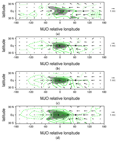
Figure 4.
Composite horizontal structure of 850 hPa wind perturbations (vectors) and precipitable water perturbations (green contours, 1 mm/day contour interval) for the mature stage of the MJO for: (a) observations; (b) the control run; (c) the 3 K warming experiment; and (d) the 7 K warming experiment. The contour interval is 1 mm, the zero contour is dotted, and negative contours are dashed. Regions with precipitation perturbations greater than 1 (3) mm/day are shaded light (dark) gray.
3.2. Changes to the MJO Resulting from Ocean Warming
When SSTs are increased, the MJO becomes more frequent, more intense, and it propagates more rapidly (Figure 1b–d). For example, with 3 K of ocean warming there are 70 MJO events during the 12-year period, compared with 40 for the control simulation, reflecting a 75 percent increase in frequency of occurrence (not shown). The rate of propagation increases from 6.4 m/s for the control run (Figure 1b) to 8.1 m/s for the 3 K ocean warming experiment (Figure 1c), to 10.3 m/s for the 7 K ocean warming run (Figure 1d). The peak amplitude of the composite precipitation signal in the rainfall time series increases from 3.9 mm/day for the control run (Figure 1b), to 5.4 mm/day for the 3 K warming experiment (Figure 1c), to 7.6 mm/day for the 7 K warming experiment simulation (Figure 1d).
Inspecting vertical and horizontal structure plots for winds and moisture (Figure 2, Figure 3 and Figure 4) reveals an amplitude increase and a slight deepening and widening of circulations. Low- to mid-level moisture perturbations, as well as precipitable water perturbations, almost double in amplitude between the control run and the 7 K warming experiment (Figure 3b,d and Figure 4b,d). Changes in the amplitude of wind perturbations are less significant (Figure 2 and Figure 4). Structural changes are quite weak for moderate ocean warming. For example, the pattern correlations between composite MJO perturbations for the control run and those for the 3 K ocean warming experiment are 0.97 and 0.98 for zonal wind (Figure 2b,c) and moisture (Figure 3b,c), respectively. With extreme ocean warming, the peak in the westerlies rises higher in the atmosphere, making it more like that in the observed MJO (Figure 2a,d). In addition to 3 K and 7 K ocean warming experiments (with results shown in Figure 1, Figure 2, Figure 3 and Figure 4), we also performed ocean warming experiments for dT = 1, 5 and 7 K. Figure 5 shows how the frequency of occurrence, amplitude, and rate of propagation of the MJO depend on the amplitude of ocean warming. In each case, there is an approximately linear relationship between the increase in ocean warming and the MJO characteristic. Frequency of occurrence (Figure 5a) deviates more from a linear relationship than the other variables (Figure 5b,c), but, considering the stochastic nature of the MJO [11], these small variations are interpreted as noise. These results suggest that the change of the MJO in response to ocean warming is for the most part systematic, and not only a consequence of random variations.
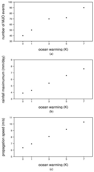
Figure 5.
Dependence of MJO characteristics on the amount of ocean warming in LAM simulations: (a) frequency of occurrence; (b) maximum rain rate in rainfall time series; and (c) propagation speed in rainfall time series.
3.3. Proposed Mechanism of MJO Amplification
Fully understanding why the MJO strengthens in response to increases in SSTs requires a knowledge of the instability mechanism of the MJO. Unfortunately, there is no scientific consensus on how this mechanism works, with different studies emphasizing different physical processes, including surface fluxes [30,31,32,33], frictionally-induced low-level convergence [34,35], and radiation [36], to name a few. While thoroughly testing the potential mechanisms of the LAM MJO is beyond the scope of this paper, the following analysis sheds light on why it intensifies in response to ocean warming.
One of the key components of the MJO’s mechanism in the LAM is the interaction of its wind perturbations with the basic state flow. Figure 6, Figure 7, Figure 8, Figure 9, Figure 10, Figure 11 and Figure 12 illustrate this point for the mature stage of the MJO. During the time when the MJO is most active in the LAM (November through May), the basic state low-level flow in in the tropics is predominately easterly, with relatively weak meridional wind components that generally converge towards the equator (Figure 6a). However, extending from the central Indian Ocean into the western Pacific, there is a narrow band of weak westerly flow centered near the equator (shaded dark gray region in Figure 6a). The MJO typically forms near the western edge of this westerly flow (note the green “I” indicating the start of initiating stage in Figure 6a), it reaches its maximum intensity near the middle of this band of westerlies (see concentric contours of rainfall for the mature stage of the MJO in green in Figure 6a), and it dissipates just to the east of these westerlies (see the green “D” for the location where the dissipating stage ends in Figure 6a). This westerly wind feature is also present in ocean warming experiments, with a similar relationship to MJO formation, maturation, and dissipation locations, although the dissipation location does shift slightly eastward as the oceans warm (Figure 6b,c). Zhang and Dong [37] noted that the observed MJO also preferentially occurs in regions with surface westerlies.
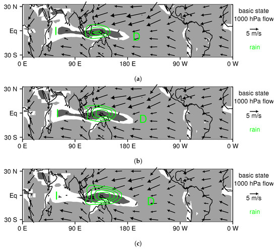
Figure 6.
Basic state 1000 hPa flow for the active season of the MJO: (a) the control simulation; (b) the 3 K warming experiment; and (c) the 7 K warming run. Regions where westerly (easterly) wind components exceed 1 m/s in amplitude are shaded dark (light) gray. Perturbation rainfall is contoured in green for 3, 5, 7, and 9 mm/day for the time when the composite MJO is in the middle of its track (i.e., at the mature stage). The letter “I” indicates the starting longitude of the initiating stage, and the letter “D” indicates the finishing longitude of the dissipating stage for the mean MJO track (i.e., the mean MJO track spans longitudes between I and D).
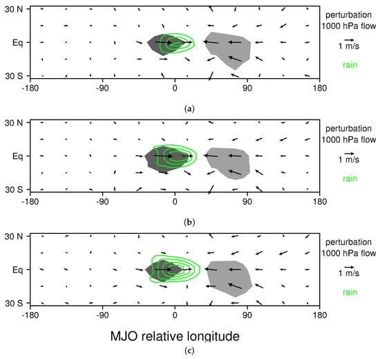
Figure 7.
MJO perturbation 1000 hPa flow in MJO relative coordinates for the mature stage of the MJO: (a) the control simulation; (b) the 3 K warming experiment; and (c) the 7 K warming run. Regions where westerly (easterly) wind components exceed 1 m/s in amplitude are shaded dark (light) gray. Perturbation rainfall is contoured in green for 3, 5, 7, and 9 mm/day.
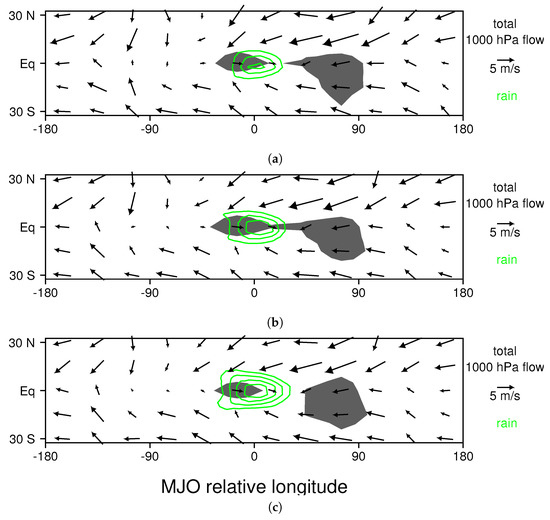
Figure 8.
Total 1000 hPa flow in MJO relative coordinates for the mature stage of the MJO: (a) the control simulation; (b) the 3 K warming experiment; and (c) the 7 K warming run. Regions in which the MJO wind perturbation causes the speed of the flow to increase by more than 1 m/s are shaded dark gray. Perturbation rainfall is contoured in green for 3, 5, 7, and 9 mm/day.
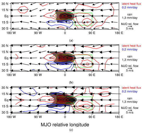
Figure 9.
Change in evaporation due to MJO wind perturbations (0.2 mm/day contour interval, with red (blue) contours denoting positive (negative) values): (a) control simulation; (b) 3 K warming experiment; and (c) 7 K warming run. Regions where perturbation rainfall exceeds 1 (3) mm/day are shaded light (dark) gray. Vectors indicate the mean low-level flow (700–1000 hPa) relative to the motion of the MJO’s precipitation center (i.e., they show how a low-level parcel would move in the MJO’s frame of reference). The average surface evaporation for the region outlined with a dotted green line, as well as it change due to ocean warming, is quantified in Figure 12a.
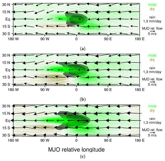
Figure 10.
Moisture change in near-surface parcels advected by MJO relative low-level flow for seven days, with green (brown) indicating moistening (drying), and the size of the box illustrating the amplitude of the change: (a) control simulation; (b) 3 K warming experiment; and (c) 7 K warming run.
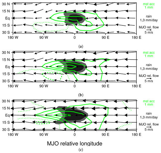
Figure 11.
Accumulated change in precipitable water resulting from surface flux perturbations and low-level advection: (a) control simulation; (b) 3 K warming experiment; and (c) 7 K warming run. The contour interval is 1 mm/day.
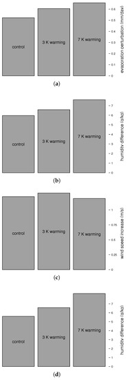
Figure 12.
Sensitivity of: (a) evaporation; (b) specific humidity difference between water surface and atmosphere; and (c) wind speed to ocean warming. For each panel, average values are shown for the region outlined with a dotted green line in Figure 9. Panel (d) shows the specific humidity difference that would occur if the lower atmospheric relative humidity and air–sea temperature difference were held constant across the simulations (i.e., how the specific humidity difference changes owing to the nonlinear nature of the Clausius–Clapeyron equation).
The composite MJO’s low-level wind perturbations include westerly flow within and just to the west of the precipitation region, and a broad region of easterlies to the east of the precipitation region (Figure 7a). This basic wind pattern, as well as its location relative to the precipitation region, is similar in the 3 K and 7 K ocean warming experiments (Figure 7b,c). The total flow, which is the sum of the basic state flow and the MJO wind perturbation, is shown in Figure 8a for the mature stage of the MJO (i.e. when it is in the middle of its track). Note that, to construct this figure, the basic state flow shown in Figure 6a was remapped to MJO-relative coordinates. For the most part, in regions where MJO wind perturbations have a significant zonal component (shaded in Figure 6b), the basic state flow has a zonal component of the same sign (Figure 6a), so that MJO wind perturbations increase the wind speed both to the east and to the west of the precipitation center (see shaded regions in Figure 8a where wind speeds are increased by more than 1 m/s). Once again, the pattern of regions with a wind speed increase are similar in the 3 K and 7 K ocean warming experiments (Figure 8b,c).
To understand the implications of these low-level wind changes, it helps to quantify their impact on moisture. Figure 9a shows how MJO wind perturbations change surface evaporation for the mature stage of the composite MJO in the control run. Red (blue) contours show regions where fluxes are enhanced (reduced) owing to an increase (decrease) in surface wind speed. There is a broad region with enhanced evaporation extending from 60 degrees west of the precipitation region to nearly 180 degrees east of the convective center, with maximum amplitudes on the order of 1 mm/day. Near the convective center and to its west enhanced evaporation is confined to a narrow band of latitudes near the equator, but to the east of the MJO enhanced evaporation spans from 30 S to 30 N. Naturally, the maxima in evaporation increases occur in the two regions where the wind speed changes are the greatest (compare Figure 8a and Figure 9a). Changes to latent heat fluxes resulting from MJO wind perturbations are for the most part positive, suggesting that surface fluxes are an important part of the instability mechanism of the MJO in the LAM. Once again, the overall pattern of surface moistening is similar in the 3 K and 7 K ocean warming experiments (Figure 9b,c), but evaporation perturbations have higher amplitudes for warmer oceans.
As discussed by Haertel et al. [23], fully understanding moistening in the MJO requires a knowledge of moisture transport in addition to local surface fluxes, because air parcels can travel long distances in just a few days to reach the convecting region of the MJO. By carefully analyzing flow pathways in two MJO events, they showed that air parcels increase in moisture and moist static energy over a period of 3–7 days prior to reaching the region of heaviest rainfall. While fully tracking air parcels (as was done in [23]) is an arduous task, and one that is difficult to complete for the many cases that go into the MJO composites used for this study, it is easy to estimate some of the immediate effects of transport by low-level winds for the composite MJO. In particular, a simple numerical experiment shows how perturbations to surface fluxes act in combination with the low-level flow to provide moisture for the MJO’s enhanced rainfall. We consider a collection of near-surface air parcels, which are initially regularly spaced on a 3 × 3 degree grid, and we then compute how the low-level wind field of the composite MJO advects them over a five-day period. For this exercise, we use the MJO-relative flow (i.e., we subtract out the MJO’s zonal propagation speed), so velocity vectors indicate how a parcel will move within the MJO’s frame of reference. For simplicity, we also make the problem two-dimensional by using the 700–1000 hPa average velocity to advect parcels (displayed as vectors in Figure 9a). In other words, we are essentially treating the parcels as columns of air. Figure 10a shows their final positions at the end of the five-day period, and it also indicates their cumulative moisture change owing to the surface flux perturbation shown in Figure 9a. Parcels shown in green (brown) have moistened (dried), with the size of the box indicating the amplitude of the moistening/drying. Figure 10a reveals that not only do surface flux perturbations enhance moisture in the vicinity of the MJO’s precipitation region, but this affect is also amplified by low-level convergence, with a dense concentration of moist parcels extending from just west of the precipitation region to southeast of the precipitation region. Once again, the patterns of moistening is similar in the ocean warming experiments (Figure 10b,c), but there is a greater degree of moistening with warmer oceans.
To further quantify the impact of low-level moistening and advection in our simple model, we calculate the change in the precipitable water that results from the enhanced surface fluxes and low-level advection, which is shown in Figure 11a. In and around the precipitation region of the MJO, there is a broad region with precipitable water increases of 1–3 mm/day. Interestingly, both the general shape of the moist anomaly and its amplitude are similar to those in the composite LAM MJO (see green contours in Figure 4b). Moreover, in our simple model, this moistening is assumed to accumulate in the lower troposphere, which is where the positive moisture anomalies are the strongest, especially to the east of the MJO’s convective center (Figure 3b). Where the pattern of moistening shown in Figure 11a is not consistent with that in composite MJO (Figure 4b), there are expected differences owing to processes the simple model neglects. For example, the model neglects the drying associated with rainfall, which could explain the tongue of moisture protruding westward of the precipitation region (Figure 11a) that is not present in composite MJO (Figure 4b). Another factor to consider is that the averaging (i.e., smoothing) used to construct the total wind field can reduce the rate of transport into the convective region. In a more rigorous analysis of moisture transport in an intense MJO event, Haertel et al. [23] noted that parcels can actually flow from west-to-east through the convecting region, although that probably does not happen in every MJO case. Another limitation of the simple model used here is that it only includes lower-tropospheric processes, which explains why the moisture anomaly extends farther eastward (Figure 11a) than it does in the composite LAM MJO in which there is a dry middle troposphere that offsets low-level moistening in terms of the precipitable water budget (Figure 3b and Figure 4b). In the ocean warming experiments, the pattern of precipitable water increases is similar to that in the control run, but both the amplitude and spatial extent of the moisture increases are greater (Figure 11b,c),
Having identified a primary moistening mechanism in the composite LAM MJO, we now turn our attention to how and why this moistening changes as the ocean warms. In the LAM, the surface flux of moisture from the ocean is proportional to both the surface wind speed and the humidity difference between the air in contact with the ocean and the air in the lower troposphere. Consequently, changes in evaporation result from a change in this humidity difference and/or a change in surface wind speed. Figure 12 shows amplitudes of evaporation, the humidity difference, and the surface wind speed for the key surface moistening region of the MJO, which is an L-shaped area outlined in dotted green in each panel of Figure 9. Evaporation increases steadily with ocean warming (Figure 12a), as does the humidity difference (Figure 12b), but there is no consistent trend in the surface wind speed (Figure 12c). We conclude that the increase in surface evaporation with warming oceans is primarily due to an increase in the humidity difference. Figure 12d shows how the specific humidity difference would change if the the air–sea temperature difference and the lower-atmospheric humidity were the same in each simulation, which is the change attributable to the non-linear nature of the Clausius–Clapeyron equation. The actual humidity difference (Figure 12c) change is slightly weaker owing to the fact that the air–sea temperature difference decreases slightly for warmer oceans.
4. Discussion
The key results presented in this paper—that ocean warming leads to a stronger MJO that is more frequent and which traverses a larger region of the tropics— are consistent with the results of the observational and modeling studies discussed above [11,12,13,14,15,17,19]. Moreover, the proposed mechanism of MJO intensification with warming oceans, enhanced surface fluxes owing to the non-linear nature of the Clausius–Clapeyron equation, is closely related to the steeper vertical gradient in moisture noted in several earlier climate warming experiments with an intensifying MJO [15,17,38]. The vertical and horizontal structure of the MJO in the LAM is also consistent with observations, both for the mature stage (e.g., Figure 2a,b, Figure 3a,b, and Figure 4a,b), and for the other stages [23]. Consequently, there is good reason to believe the LAM MJO has a similar mechanism to the MJO in nature, and this mechanism will contribute to the strengthening of the MJO in the future provided that the oceans continue to warm.
However, several limitations to the results presented here should be mentioned. In particular, the model lacks several feedbacks that would likely reduce the amount of MJO intensification if included, especially for the cases with strong prescribed ocean warming. First, owing to the experimental set-up with prescribed SSTs, there is no feedback to cool the ocean when surface evaporation is enhanced. Second, twin cyclones often form within strong MJOs, which can weaken the eastward propagating component of the MJO [23], and this process in not well resolved by the LAM experiments. Third, the LAM experiments artificially constrain the structure of SST patterns to remain the same, and this would likely change in a realistic ocean warming scenario. The interpretation that MJO intensification results from changes to surface fluxes also has limitations as well. In particular, surface flux enhancement only occurs to the east of the MJO’s convective center when the MJO’s perturbation easterlies line up with basic state easterlies, which happens during much of the mature and dissipating stages of the MJO, but not during the initiation stage when the MJO is over the western Indian Ocean. Other processes, such as radiation [36], circumnavigating Kelvin waves [24], zonal wind perturbations interacting with basic state moisture gradients, and/or extratropical forcing [39] likely help to intensify the MJO in the western Indian Ocean, and possibly anchor its initiation there even when surface westerlies weaken in the extreme warming scenario (Figure 6c). Finally, the LAM’s radiation scheme is quite idealized, with the infrared optical depth largely determined by the atmospheric precipitable water [22,23,24], and only a crude representation of cloud radiative effects. In particular, it does not capture changes to optical depth resulting from carbon dioxide increases, which could lead to an inaccurate balance between ocean and land heating when it is applied in ocean warming scenarios, and which might also affect the intensity of the MJO.
The author’s conceptual interpretation of the MJO’s intensification mechanism has similarities to a combination of the original wind induced surface heat exchange theories of Emanuel [30] and Neelin and Held [31] and the more recent models of Sobel and Maloney [32,33]. Those theories assumed that the MJO’s perturbation winds either enhanced surface fluxes in regions with basic state easterlies or westerlies. The actual basic state winds in the environment of the MJO (both in the LAM and in nature) includes both easterlies and westerlies, with a structure that depends on both latitude and longitude (Figure 6 [37]), and the way the MJO perturbations interact with the basic state differs by region (Figure 7 and Figure 8). Moreover, as illustrated in Figure 9, Figure 10 and Figure 11 and by the parcel tracking analysis of [23], transport of moisture by low-level winds is also important, leading to convective heating occurring at locations far removed from surface moistening, unlike most moisture mode theories of the MJO assume. The author’s conceptual model of MJO moistening has several differences from the recent model of Adames and Kim [40], which has no zonal variation in basic state winds, does not include advection of moisture perturbations by perturbation winds, and which relies more heavily on cloud radiative effects than surface fluxes to destabilize the MJO. In fact, even when cloud radiative interactions are turned off in the LAM, a robust MJO is present with nearly identical structure in a composite sense, although it does become slightly weaker and less frequent (not shown). In addition, the author’s understanding of the MJO is not consistent with the idea that frictional convergence is essential to the MJO’s mechanism [34,35]. The MJO’s perturbation wind field is dominated by zonal convergence, with little if any consistent signal of an increase in meridional convergence in the precipitation region (Figure 7), which would be necessary to explain the MJO’s rainfall perturbation from a frictional convergence mechanism.
The surface moistening analysis has provided a plausible explanation for why the LAM MJO produces heavier rainfall with warmer oceans; however, two other changes in the MJO present in warmer ocean experiments are not explained (e.g., Figure 1b,c): (1) the MJO’s path spans a larger region of the tropics; and (2) the propagation speed of the MJO increases. Considering that the presence of the narrow, equatorial band of basic state westerlies is what allows MJO perturbation westerlies to enhance surface fluxes of moisture (Figure 6, Figure 7, Figure 8 and Figure 9), it is tempting to suggest that the MJO propagates farther eastward in ocean warming experiments because the basic state surface westerly winds extends farther eastward (Figure 6). However, it is also possible that the causality works the other way, and that the basic state westerlies extend farther eastward in the ocean warming experiments because the MJO is stronger and propagates farther eastward. Similarly, quantitatively explaining the increase in phase speed is not straightforward, and will likely require considering not only changes to surface evaporation, but also changes to the basic state moisture field and their interaction with MJO wind perturbations [24,38,41].
5. Conclusions
In this study, the author explores how the Madden Julian Oscillation (MJO) responds to ocean warming using a Lagrangian Atmospheric Model (LAM). A series of 12-year simulations are carried out with the LAM, each forced with an observed SST pattern increased by a constant amount dT, where dT = 0, 1, 3, 5, 7 K. For each simulation, MJOs are identified by tracking large-scale eastward-propagating precipitation anomalies in time-filtered equatorial rainfall data, and a composite MJO is created.
As the oceans warm, the MJO becomes more frequent and intense, it propagates more rapidly, and its path covers a larger portion of the Indian and Pacific Oceans. An analysis of how MJO wind perturbations combine with basic state winds reveals that surface flux enhancement by MJO wind perturbations is a key component of the LAM MJO. The moistening from surface fluxes increases as the ocean warms, largely because of the non-linear nature of the Clausius–Clapyron equation, which is suggested as a mechanism of MJO intensification.
Acknowledgments
This research was supported by NSF grant AGS-1561066
Conflicts of Interest
The author declares no conflict of interest.
References
- Madden, R.A.; Julian, P.R. Detection of a 40–50 day oscillation in the zonal wind in the tropical Pacific. J. Atmos. Sci. 1971, 28, 702–708. [Google Scholar] [CrossRef]
- Madden, R.A.; Julian, P.R. Description of global-scale circulation cells in the tropics with a 40–50 day period. J. Atmos. Sci. 1972, 29, 1109–1123. [Google Scholar] [CrossRef]
- Madden, R.A.; Julian, P.R. Observations of the 40–50-day tropical oscillation—A review. Mon. Weather Rev. 1994, 122, 814–837. [Google Scholar] [CrossRef]
- Kiladis, G.N.; Straub, K.H.; Haertel, P.T. Zonal and vertical structure of the Madden–Julian oscillation. J. Atmos. Sci. 2005, 62, 2790–2809. [Google Scholar] [CrossRef]
- Wu, M.L.C.; Schubert, S.; Huang, N.E. The development of the South Asian summer monsoon and the intraseasonal oscillation. J. Clim. 1999, 12, 2054–2075. [Google Scholar] [CrossRef]
- Lorenz, D.J.; Hartmann, D.L. The effect of the MJO on the North American monsoon. J. Clim. 2006, 19, 333–343. [Google Scholar] [CrossRef]
- Liebmann, B.; Hendon, H.H.; Glick, J.D. The relationship between tropical cyclones of the western Pacific and Indian Oceans and the Madden-Julian oscillation. J. Meteorol. Soc. Jpn. Ser. II 1994, 72, 401–412. [Google Scholar] [CrossRef]
- Maloney, E.D.; Hartmann, D.L. Modulation of eastern North Pacific hurricanes by the Madden–Julian oscillation. J. Clim. 2000, 13, 1451–1460. [Google Scholar] [CrossRef]
- Fedorov, A.V.; Hu, S.; Lengaigne, M.; Guilyardi, E. The impact of westerly wind bursts and ocean initial state on the development, and diversity of El Niño events. Clim. Dyn. 2015, 44, 1381–1401. [Google Scholar] [CrossRef]
- Puy, M.; Vialard, J.; Lengaigne, M.; Guilyardi, E. Modulation of equatorial Pacific westerly/easterly wind events by the Madden–Julian oscillation and convectively-coupled Rossby waves. Clim. Dyn. 2016, 46, 2155–2178. [Google Scholar] [CrossRef]
- Slingo, J.; Rowell, D.; Sperber, K.; Nortley, F. On the predictability of the interannual behaviour of the Madden-Julian Oscillation and its relationship with El Niño. Q. J. R. Meteorol. Soc. 1999, 125, 583–609. [Google Scholar] [CrossRef]
- Jones, C.; Carvalho, L.M. Changes in the activity of the Madden–Julian oscillation during 1958–2004. J. Clim. 2006, 19, 6353–6370. [Google Scholar] [CrossRef]
- Jones, C.; Carvalho, L.M. Stochastic simulations of the Madden–Julian oscillation activity. Clim. Dyn. 2011, 36, 229–246. [Google Scholar] [CrossRef]
- Takahashi, C.; Sato, N.; Seiki, A.; Yoneyama, K.; Shirooka, R. Projected future change of MJO and its extratropical teleconnection in east Asia during the northern winter simulated in IPCC AR4 models. SOLA 2011, 7, 201–204. [Google Scholar] [CrossRef]
- Arnold, N.P.; Branson, M.; Kuang, Z.; Randall, D.A.; Tziperman, E. MJO intensification with warming in the superparameterized CESM. J. Clim. 2015, 28, 2706–2724. [Google Scholar] [CrossRef]
- Grabowski, W.W. Coupling cloud processes with the large-scale dynamics using the cloud-resolving convection parameterization (CRCP). J. Atmos. Sci. 2001, 58, 978–997. [Google Scholar] [CrossRef]
- Carlson, H.; Caballero, R. Enhanced MJO and transition to superrotation in warm climates. J. Adv. Model. Earth Syst. 2016, 8, 304–318. [Google Scholar] [CrossRef]
- Song, E.J.; Seo, K.H. Past-and present-day Madden-Julian Oscillation in CNRM-CM5. Geophys. Res. Lett. 2016, 43, 4042–4048. [Google Scholar] [CrossRef]
- Adames, A.F.; Kim, D.; Sobel, A.H.; Del Genio, A.; Wu, J. Changes in the structure and propagation of the MJO with increasing CO2. J. Adv. Model. Earth Syst. 2017, 9, 1251–1268. [Google Scholar] [CrossRef] [PubMed]
- Haertel, P.T.; Straub, K.H. Simulating convectively coupled Kelvin waves using Lagrangian overturning for a convective parametrization. Q. J. R. Meteorol. Soc. 2010, 136, 1598–1613. [Google Scholar] [CrossRef]
- Haertel, P. A Lagrangian method for simulating geophysical fluids. In Lagrangian Modeling of the Atmosphere; American Geophysical Union: Washington, DC, USA, 2012; pp. 85–98. [Google Scholar]
- Haertel, P.; Straub, K.; Fedorov, A. Lagrangian overturning and the Madden–Julian Oscillation. Q. J. R. Meteorol. Soc. 2014, 140, 1344–1361. [Google Scholar] [CrossRef]
- Haertel, P.; Boos, W.R.; Straub, K. Origins of Moist Air in Global Lagrangian Simulations of the Madden–Julian Oscillation. Atmosphere 2017, 8, 158. [Google Scholar] [CrossRef]
- Haertel, P.; Straub, K.; Budsock, A. Transforming circumnavigating Kelvin waves that initiate and dissipate the Madden–Julian Oscillation. Q. J. R. Meteorol. Soc. 2015, 141, 1586–1602. [Google Scholar] [CrossRef]
- Claussen, M.; Mysak, L.; Weaver, A.; Crucifix, M.; Fichefet, T.; Loutre, M.F.; Weber, S.; Alcamo, J.; Alexeev, V.; Berger, A.; et al. Earth system models of intermediate complexity: closing the gap in the spectrum of climate system models. Clim. Dyn. 2002, 18, 579–586. [Google Scholar]
- Taylor, K.E.; Stouffer, R.J.; Meehl, G.A. An overview of CMIP5 and the experiment design. Bull. Am. Meteorol. Soc. 2012, 93, 485–498. [Google Scholar] [CrossRef]
- Hung, M.P.; Lin, J.L.; Wang, W.; Kim, D.; Shinoda, T.; Weaver, S.J. MJO and convectively coupled equatorial waves simulated by CMIP5 climate models. J. Clim. 2013, 26, 6185–6214. [Google Scholar] [CrossRef]
- Durre, I.; Vose, R.S.; Wuertz, D.B. Overview of the integrated global radiosonde archive. J. Clim. 2006, 19, 53–68. [Google Scholar] [CrossRef]
- Huffman, G.J.; Adler, R.F.; Arkin, P.; Chang, A.; Ferraro, R.; Gruber, A.; Janowiak, J.; McNab, A.; Rudolf, B.; Schneider, U. The global precipitation climatology project (GPCP) combined precipitation dataset. Bull. Am. Meteorol. Soc. 1997, 78, 5–20. [Google Scholar] [CrossRef]
- Emanuel, K.A. An air-sea interaction model of intraseasonal oscillations in the tropics. J. Atmos. Sci. 1987, 44, 2324–2340. [Google Scholar] [CrossRef]
- Neelin, J.D.; Held, I.M. Modeling tropical convergence based on the moist static energy budget. Mon. Weather Rev. 1987, 115, 3–12. [Google Scholar] [CrossRef]
- Sobel, A.; Maloney, E. An idealized semi-empirical framework for modeling the Madden–Julian oscillation. J. Atmos. Sci. 2012, 69, 1691–1705. [Google Scholar] [CrossRef]
- Sobel, A.; Maloney, E. Moisture modes and the eastward propagation of the MJO. J. Atmos. Sci. 2013, 70, 187–192. [Google Scholar] [CrossRef]
- Wang, B.; Rui, H. Dynamics of the coupled moist Kelvin–Rossby wave on an equatorial β-plane. J. Atmos. Sci. 1990, 47, 397–413. [Google Scholar] [CrossRef]
- Maloney, E.D.; Hartmann, D.L. Frictional moisture convergence in a composite life cycle of the Madden–Julian oscillation. J. Clim. 1998, 11, 2387–2403. [Google Scholar] [CrossRef]
- Raymond, D.J. A new model of the Madden–Julian oscillation. J. Atmos. Sci. 2001, 58, 2807–2819. [Google Scholar] [CrossRef]
- Zhang, C.; Dong, M. Seasonality in the Madden–Julian oscillation. J. Clim. 2004, 17, 3169–3180. [Google Scholar] [CrossRef]
- Adames, Á.F.; Kim, D.; Sobel, A.H.; Del Genio, A.; Wu, J. Characterization of moist processes associated with changes in the propagation of the MJO with increasing CO2. J. Adv. Model. Earth Syst. 2017, 9, 2946–2967. [Google Scholar] [CrossRef] [PubMed]
- Straus, D.M.; Lindzen, R.S. Planetary-scale baroclinic instability and the MJO. J. Atmos. Sci. 2000, 57, 3609–3626. [Google Scholar] [CrossRef]
- Adames, Á.F.; Kim, D. The MJO as a dispersive, convectively coupled moisture wave: Theory and observations. J. Atmos. Sci. 2016, 73, 913–941. [Google Scholar] [CrossRef]
- Pritchard, M.S.; Bretherton, C.S. Causal evidence that rotational moisture advection is critical to the superparameterized Madden–Julian oscillation. J. Atmos. Sci. 2014, 71, 800–815. [Google Scholar] [CrossRef]
© 2018 by the author. Licensee MDPI, Basel, Switzerland. This article is an open access article distributed under the terms and conditions of the Creative Commons Attribution (CC BY) license (http://creativecommons.org/licenses/by/4.0/).