Cluster Analysis of Monthly Precipitation over the Western Maritime Continent under Climate Change

Abstract

Changes in climate because of global warming during the 20th and 21st centuries have a direct impact on the hydrological cycle as driven by precipitation. However, studying precipitation over the Western Maritime Continent (WMC) is a great challenge, as the WMC has a complex topography and weather system. Understanding changes in precipitation patterns and their groupings is an important aspect of planning mitigation measures to minimize flood and drought risk as well as of understanding the redistribution of precipitation arising from climate change. This paper employs Ward’s hierarchical clustering on regional climate model (RCM)-simulated monthly precipitation gridded data over 42 approximately evenly distributed grid stations from the years 2030 to 2060. The aim was to investigate spatial and temporal groupings over the four major landmasses in the WMC and to compare these with historical precipitation groupings. The results showed that the four large-scale islands of Java, Sumatra, Peninsular Malaysia and Borneo would experience a significant spatial redistribution of precipitation over the years 2030 to 2060, as compared to historical patterns from 1980 to 2005. The spatial groups were also compared for two future forcing scenarios, representative concentration pathways (RCPs) 4.5 and 8.5, and different groupings over the Borneo region were observed.

1. Introduction

Climate change during the 20th and 21st centuries because of global warming has directly influenced precipitation all over the world. Most reported studies [1,2,3,4] focus on the changes in intensity and frequency of precipitation because of climate change, while there is significantly less research on the effect of climate change on the redistribution of precipitation. The redistribution of precipitation within regions and seasons is an important aspect of climate change, as it poses a high risk to agriculture [5], water security [6], as well as an increased chance of floods and droughts [7,8]. Also, site selection for the construction of hydrological and hydraulic structures such as drains, dams and reservoirs is dependent on precipitation distribution within a region [9,10]. The redistribution of precipitation in the future can make these structures less useful and sometimes even redundant [11,12].

The alterations and variability in future precipitation are traditionally studied using outputs from global climate models (GCMs) [13,14,15,16]. However, GCMs have a low resolution, typically 1.5° to 2.5°, and in order to mitigate impacts of future precipitation, their output needs to be able to focus on the regional or local scale [14,17]. Regional- or local-scale data can be achieved using dynamical downscaling, in which regional climate models (RCMs) are implemented to downscale GCM data to a higher grid resolution.

The weather research and forecasting (WRF) model is one such RCM and is used here to study future precipitation groups and patterns for the Western Maritime Continent (WMC). WMC precipitation is highly influenced by prominent convection in the region [18,19,20], as well as its complex topography. Also, since the WMC is a homogeneous air mass and has evenly distributed pressure and sea-surface temperatures, the weather and climate in this region are heavily dependent on local and mesoscale factors [21]. The WMC encompasses four large-scale islands: Java, Sumatra, Peninsular Malaysia and Borneo, and also has a multitude of smaller islands, many of which are mountainous [21,22]. Grouping precipitation patterns can provide a concise and structural summary of climate in the region. Thus, the objective of this work is to identify spatial and temporal patterns of monthly precipitation over the WMC using Ward’s clustering algorithm [23,24].

Statistical methods are effective for spatiotemporal characterization in meteorology and help to identify precipitation groupings. Several studies to characterize spatiotemporal data, such as principal component analysis to model diurnal rainfall over the Maritime Continent [25], empirical orthogonal functions to characterize the spatial variability of monthly rainfall over India [26], and k-nearest-neighbor to simulate daily precipitation [27] have been implemented. However, most of these clustering methods require the number of clusters or components to be inputted. Specifying an incorrect number of clusters can result in substantial errors in the analysis [28,29]. To overcome this, the present study implements hierarchical clustering, using Ward’s cluster analysis (CA) method, which does not require pre-specification of the number of input clusters [30,31]. Thus, CA contributes to the identification of unusual patterns or groups and links within the data [32]. CA is recognized as an effective tool for identifying homogeneous groupings of stations with respect to their climatology. Furthermore, Blashfield [33] showed that Ward’s CA method generated the most accurate results among four hierarchical clustering methods tested.

Previous studies primarily grouped the climatology of the major islands within the WMC based on their geographical location. For example, Peninsular Malaysia was divided into four regions, i.e., Northern, Central, Eastern and Southern [34,35]. The Northern region was reported to receive the highest precipitation from September to October, the Central from October to November, the Eastern from November to December, and the Southern from December to January. More precisely, the Indonesian Bureau of Meteorology, Climatology, and Geophysics (BMKG) [36] classified Indonesia into 293 areas with different precipitation characteristics to reflect the complexity and heterogeneity of precipitation distribution [37]. However, these groupings were based on the historical observed and modelled data, and thus may not hold in future, under alterations in the hydrological cycle resulting from climate change effects.

The goal of this work is to apply Ward’s hierarchical clustering on monthly precipitation data obtained from WRF modeling over the WMC. The WRF model was driven using the Coupled Model Intercomparison Project Phase 5 (CMIP5) GCM data and bias-corrected with the observed Climate Hazards Group InfraRed Precipitation with Station (CHIRPS) dataset. The methodology was applied for 42 distributed stations (locations) as shown in Figure 1. The objectives behind clustering the precipitation data were: (i) to discover spatial grouping of precipitation distribution within the WMC under the present and future climate; and (ii) to uncover the monthly and seasonal precipitation cycle for each cluster. The author believes this is the first such study using CA over the WMC.

2. Study Area and Datasets

2.1. Study Area

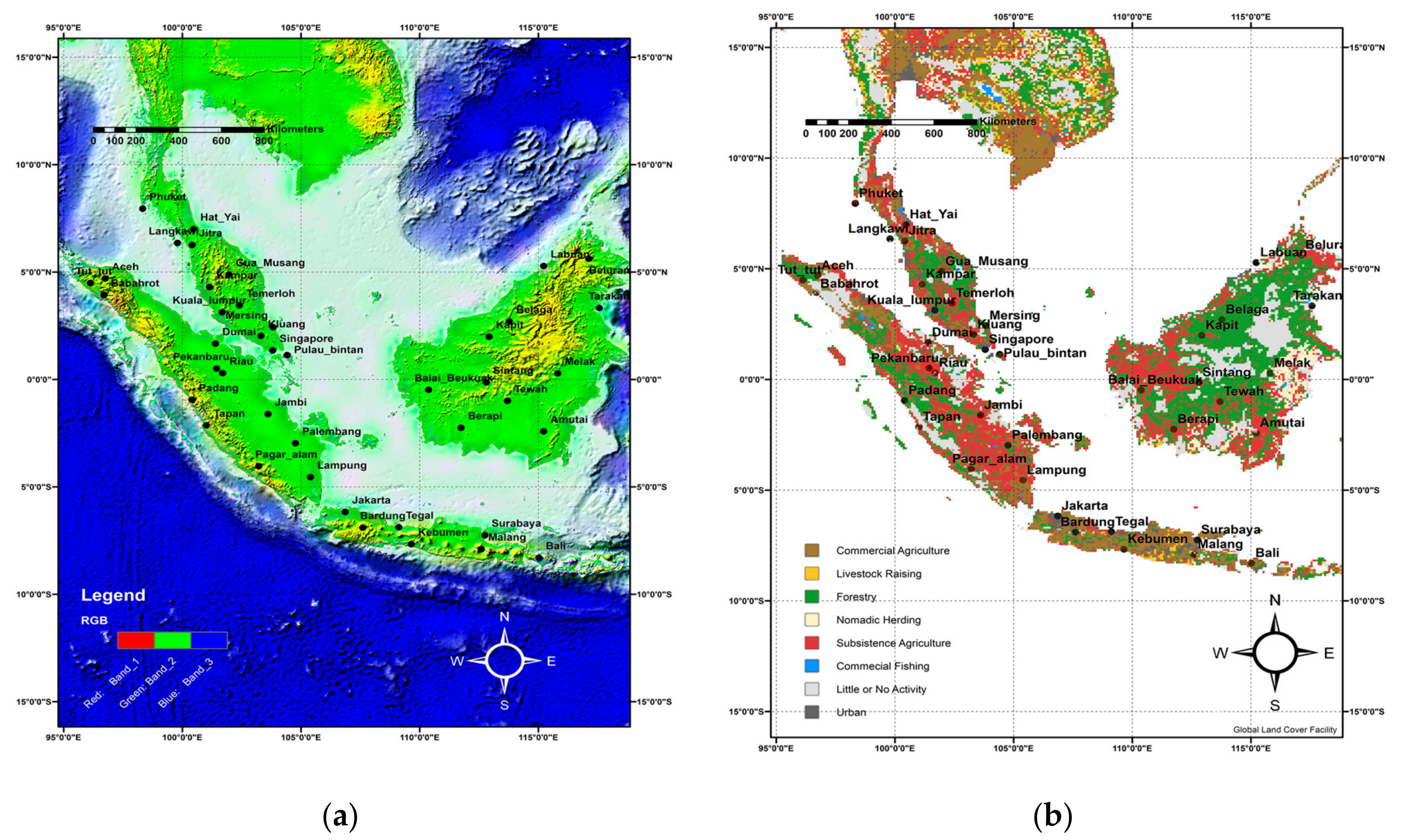
The WMC is the western part (900 E to 1200 E and 100 S to 100 N) of the Maritime region as defined by Ramage [21,38]. Figure 2a,b show the complex topography and mixed land-use patterns, respectively, of the WMC. A total of 42 distributed “stations” (the locations are listed in

Table 1. Stations, coordinates (latitude and longitude), altitude and land use of the locations used in this study. Time range of the monthly data is from January 1981 to December 2016.

Number	Location	Latitude (°)	Longitude (°)	Altitude (m)	Land Use	Mean Annual Precipitation (mm/day)
Java
1	Jakarta	−6.17	106.87	9	Urban	4.87
2	Bardung	−6.9	107.61	704	Urban	5.61
3	Surabaya	−7.25	112.75	9	Urban	4.66
4	Bali	−8.3	115.03	1491	Com Agr	7.38
5	Malang	−7.9	112.6	458	Urban	6.25
6	Tegal	−6.879	109.12	9	Sub Agr	5.5
7	Kebumen	−7.6681	109.65	57	Com Agr	10.13
Sumatra
8	Riau	0.2933	101.7	6	Sub Agr	7.71
9	Jambi	−1.6101	103.613	45	Sub Agr	5.9
10	Lampung	−4.55	105.4	32	Com Agr	7.45
11	Pagar alam	−4.04	103.22	794	Sub Agr	7.54
12	Padang	−0.947	100.41	59	Forestry	10.05
13	Tapan	−2.14	101.025	18	Sub Agr	10.66
14	Pekanbaru	0.507	101.447	10	Sub Agr	7.36
15	Aceh	4.6951	96.749	1061	Forest	4.94
16	Dumai	1.666	101.4	14	LA/NA	6.63
17	Palembang	−2.97	104.77	2	Forest	7.09
18	Babahrot	3.93	96.7	67	Com Agr	7.7
19	Tut tut	4.49	96.13	104	Forest	9.69
Independent Islands
20	Singapore	1.3521	103.81	58	Urban	6.33
21	Pulau Bintan	1.136	104.42	27	Urban	7.28
Malaysia
22	Kuala lumpur	3.13	101.68	59	Urban	7.26
23	Kluang	2.03	103.318	23	Forest	6.37
24	Mersing	2.43	103.83	9	Forest	6.84
25	Temerloh	3.448	102.41	59	Sub Agr	5.79
26	Kampar	4.3	101.15	23	Forest	9.41
27	Gua Musang	4.88	101.96	87	Forest	8.84
28	Jitra	6.264	100.42	7	Com Agr	6.45
29	Langkawi	6.35	99.8	49	Sub Agr	6.85
30	Phuket	7.95	98.33	326	Sub Agr	6.71
31	Hat Yai	7	100.47	11	Sub Agr	5.57
Borneo
32	Labuan	5.28	115.23	27	Urban	8.78
33	Kapit	1.99	112.93	39	Forest	11.05
34	Amutai	−2.4166	115.23	16	Sub Agr	7.22
35	Melak	0.286	115.82	8	Forest	8.92
36	Belaga	2.7	113.78	48	Forest	10.36
37	Beluran	5.62	117.13	97	LA/NA	10.88
38	Tarakan	3.327	117.57	25	LA/NA	10.46
39	Sintang	−0.137	112.81	579	LA/NA	9.87
40	Balai Beukuak	−0.48	110.38	203	Forest	8.99
41	Berapi	−2.25	111.75	70	Sub Agr	8.48
42	Tewah	−1	113.7	65	Forest	9.56

) were selected for the cluster analysis. Note that “stations” here actually refers to overall grid precipitation, although the grids are high resolution, being 25 km for CHIRPS and WRF–CMIP5. The stations were strategically chosen within the four major islands in the WMC, specifically from Sumatra (12), Java (7), Malaysia (10), Borneo (12) and the Independent Islands (2). Table 1 categorizes the islands from where the grid locations are selected along with their coordinates, altitude, mean annual precipitation, and land use, characterized into eight categories (i.e., commercial agriculture (Com Agr), livestock-raising, forest, nomadic herding, subsistence agriculture (Sub Agr), commercial fishing, little or no activity (LA/NA and urban).

2.2. Dataset Used

2.2.1. Coupled Model Intercomparison Project Phase 5 (CMIP5) and Weather Research and Forecasting (WRF)

The boundary and initial conditions needed for WRF runs were provided by CMIP5 Community Earth System Model (CESM) bias-corrected data (ds316.1 dataset). This dataset was built in accordance with the Intergovernmental Panel on Climate Change (IPCC) [39,40], by bias correcting the outputs from Version 1 of CESM, by Research Data Archive (RDA), using European Centre for Medium-Range Weather Forecasts (ECMWF) Interim Reanalysis (ERA-Interim) from 1981 to 2005. Here, CESM is a coupled GCM that has four different model components simulating atmosphere, ocean, sea-ice and land surface, corresponding to different representative concentration pathways (RCPs).

The CMIP5 ds316.1 dataset was downscaled using WRF to 25 km grid resolution for the years 1980–2005 (historical) and 2030–2060 (future) under RCP 4.5 and RCP 8.5. This was the most computationally intensive part of the work, where more than 88 years (26 historical years and 31 years each for RCP 4.5 and RCP 8.5) of WRF runs were done using the parameterization scheme described in Section 3.

2.2.2. Climate Hazards Group InfraRed Precipitation with Station (CHIRPS) Dataset

CHIRPS is a long-period dataset that employs a “smart” interpolation technique on infrared cold-cloud distribution to estimate precipitation [41]. CHIRPS is built on 5 km climatology that includes daily, as well as monthly, precipitation from the year 1981 to the present. CHIRPS data is used as the observed dataset, for bias. Furthermore, CHIRPS also has a long time range (January 1981–December 2016). The spatial resolution of the WRF monthly precipitation data was 25 km. Hence, the CHIRPS 5 km data was bi-linearly averaged to 25 km to match the WRF resolution.

3. Methodology

3.1. Parametrization of WRF

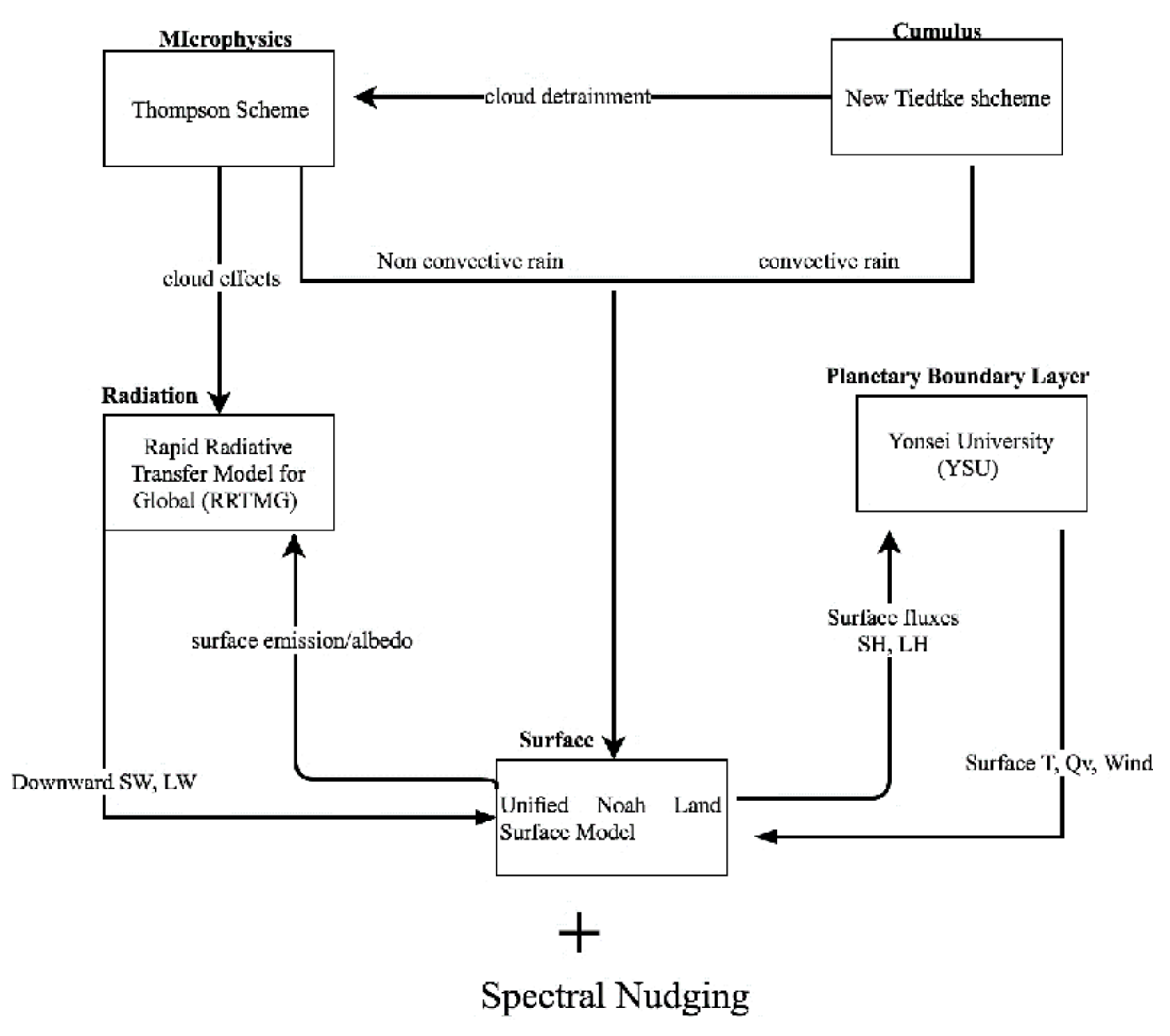
The WRF physics parametrizations implemented in this study are shown in Figure 3 along with their interactions within the model. The WRF parametrization was performed using a Thomson microphysics scheme [42]. Shortwave (SW) and longwave (LW) radiation modeling was parametrized using the Rapid Radiative Transfer Model for Global (RRTMG) [43]. The Yonsei University (YSU) model [44] was the planetary boundary layer scheme used, and the land-surface model was parametrized using the Noah land-surface model [45]. The new Tidtke scheme was the cumulus scheme used in this study to resolve precipitation resulting from convection [46]. The biases within the WRF model for long climate runs were minimized by activating spectral nudging for long waves.

3.2. Performance of WRF in Modeling Precipitation over Study Domain

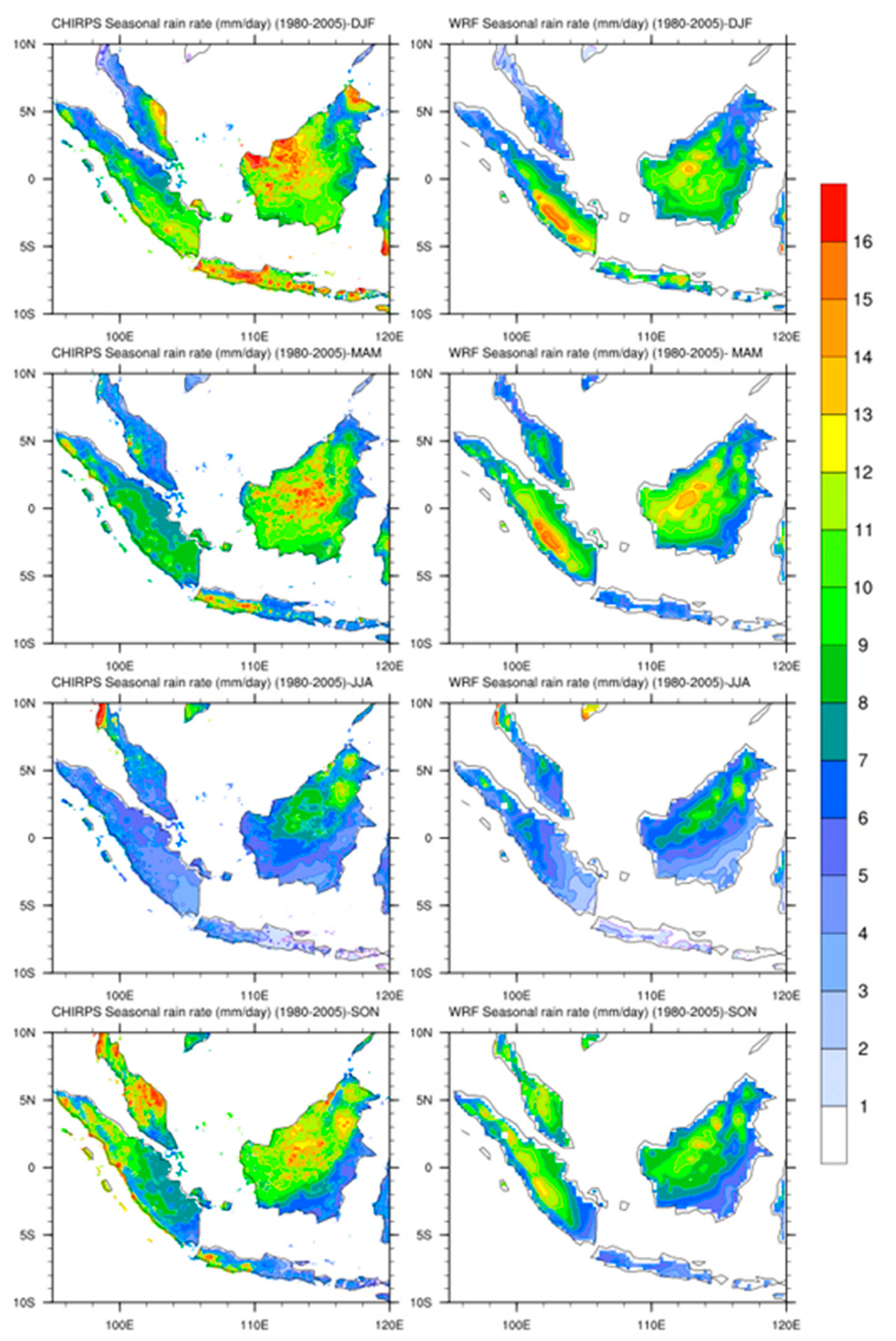
The above parametrization scheme enabled the WRF model to capture precipitation accurately in all seasons. As noted above, the WRF model (25 km grid output) was checked using a comparison with CHIRPS data (5 km grid) (see Figure 4). A smaller magnitude of precipitation in many areas was expected, as the 25-km grid could not have captured sub-grid processes. However, it was observed that the simulated precipitation from the WRF parametrization captured details that could have been only resolved by higher resolution data. For example, excess precipitation resulting from the Borneo vortex was, unexpectedly, quite accurately captured by the WRF parametrization scheme.

It was observed that the WRF–CMIP5 simulated precipitation was very close to CHIRPS for all seasons and regions, even on the elevated terrain of Sumatra and Java, which are typically over-exaggerated by RCMs. The WRF model bias percentage in seasonal precipitation, i.e., $\frac{\left(model - observed\right)}{observed} \times 100$ where observed data were from the CHIRPS data (bi-linearly averaged to 25 km) is plotted in Figure 5a,b. The overall bias plot (see Figure 5a) shows that the WRF-modelled data had a low bias compared to CHIRPS. However, some of the regions in the eastern Malaysian peninsula (for the months DJF and MAM) and western Sumatra (for SON) showed a higher bias percentage in the range of 45% during the dry periods. This bias with respect to the maximum value in the region is plotted in Figure 5b, which shows a much lower bias percentage, confirming that the higher percentage observed in Figure 5a was the result of low precipitation.

3.3. Bias Correction of the WRF Dataset

As the comparison for WRF–CMIP5 was made with historical data, it was important to normalize the model biases for future data extracted from WRF. The bias correction of the 25 km–scale monthly WRF–CMIP5 model was done using gamma quantile mapping (GQM) [47]. The GQM bias-correction method is based on the initial assumption that both observed and simulated intensity distributions are well approximated by the gamma distribution:

$$pdf\left(x\right)= \frac{e^{\left(\frac{-x}{\theta }\right)}{x}^{k-1}}{\Gamma \left(k\right){\theta }^k}.$$

(1)

Here, x is the normalized monthly precipitation, k and θ are the form and scaling parameters, respectively, and Γ(k) = (k − 1)! Considering precipitation having k > 1 and following the distribution shown in Equation 1 is a general practice in hydrology [48,49,50,51]. However, when precipitation has k = 1 (i.e., exponential distribution) or k < 1 (dry months), the GQM cannot be applied. The dry months are added to the parameters by providing a threshold value for dry months [47].

The GQM method is an efficient bias-correction method as it considers both mean and extreme precipitation while bias-correcting the precipitation [47,52,53]. It is observed that GQM filters out the extreme values that are results of errors while keeping the extreme values that are likely to be genuine. This makes GQM preferable over the conventional quantile mapping and scaling methods that do not distinguish between the extreme values resulting from noise or extreme climate conditions [54]. However, the accuracy of the GQM model is highly dependent on the period over which the data is trained, i.e., the larger the training period, the greater precision. In this study, the monthly historical data extracted from WRF was bias corrected with historical 25 km CHIRPS data using the GQM method for a period of 26 years (1980–2005). The bias-correction factor achieved from the historical datasets is mapped to the WRF–CMIP5 future dataset. Therefore, hereafter WRF–CMIP5 stands for the bias-corrected WRF–CMIP5 dataset.

3.4. Cluster Analysis (Ward’s Method)

The method proposed by [24], “Ward’s Hierarchical Clustering” or the “method of minimum variance,” was used in this study. The method was used to group locations and their monthly precipitation distributions based on their similarity. Ward’s method looks at cluster analysis as a variance problem, and computes Euclidean distances to evaluate dissimilarity between the clusters. Equation (2) gives the formula for calculating Euclidian distance as:

$$d_e={\left[{\sum }_{j=1}^n{\left(P_{a,j} - P_{b,j}\right)}^2\right]}^{0.5}.$$

(2)

where P_a,j and P_b,j are the quantitative variable j (monthly precipitation in this study) from stations a and b, respectively. Ward’s algorithm, when implemented on a dataset, establishes groups by minimizing the dissimilarity or the total sum of squares (TSS):

$$\mathrm{TSS} = {\sum }_{j=1}^n{\left(P_{a,j} - P_{b,j}\right)}^2.$$

(3)

The final clusters have minimum TSS within each cluster. Ward’s algorithm calculates several clusters at a level when intergroup similarity is maximized while intragroup similarity is minimized.

Ward’s method, when implemented for precipitation, uses the coefficient of variation (CV) and the mean value for the monthly precipitation. The values for CV and mean were organized in two configuration matrices pnp. Each matrix pnp had mean (or CV) in its rows (n) and the station (p) in the columns. These configuration matrices were used to identify clusters of similar stations. Furthermore, precipitation within these clusters was analyzed to discover the monthly (i.e., temporal) patterns or seasonality within the spatial cluster. For the second step, the mean (or CV) were arranged in rows for matrix pnp, and months were set up in columns (p). The Ward’s clustering method used in this paper was implemented directly using the “stats” package [55] in R programming language.

4. Results

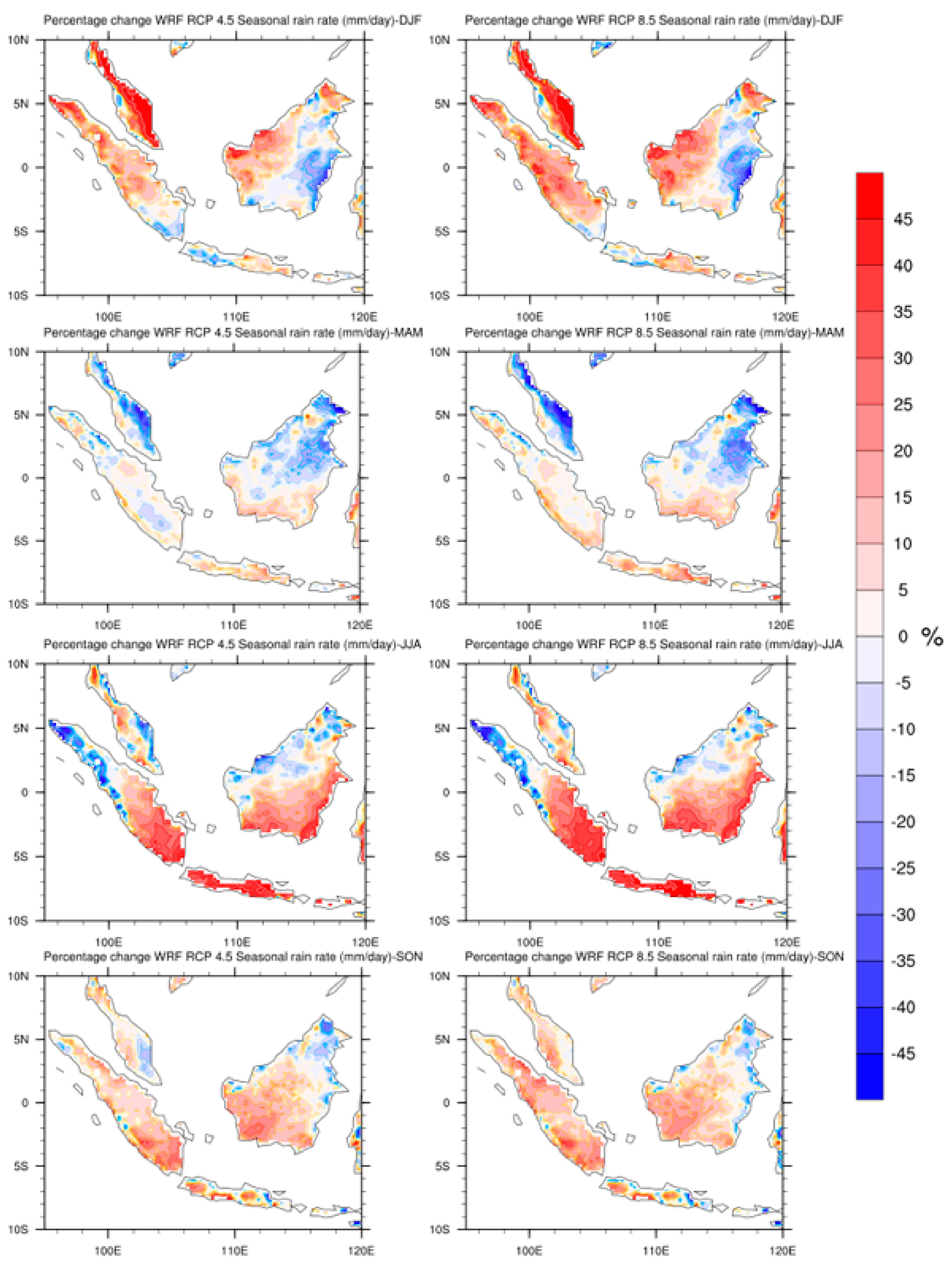
The future seasonal precipitation rate from WRF–CMIP5 was yearly averaged over the period 2030–2060, while the historical period was 1980–2005. As seen in Figure 6, a significant change in precipitation rate was observed for the future scenarios as compared to the historical period for all seasons. In Figure 6, both future and historical modeled precipitation are bias-corrected using the same bias correction developed for the historical-modeled output, based on the observed CHIRPS data. The bias correction removed the uncertainty resulting from the model; retaining, however, the uncertainty resulting from climate change forcing (RCP 4.5 and RCP 8.5 in this study). Thus, the change in future precipitation is presented in a consistent way. The maximum changes in mean seasonal precipitation rate ~45% were observed for Peninsular Malaysia and Java for the DJF season, as well as southern Sumatra for the season JJA. Seasons MAM and SON showed minimum changes. Interestingly, many regions in the WMC may also experience a decline in mean precipitation rate in future scenarios; for example, south-east Borneo in DJF and MAM, as well as western Sumatra and Malay Peninsular in MAM. However, as most of the reported studies, e.g., Lehmann [56] indicated that global warming is already increasing the odds of extreme precipitation events, it is of much more relevance to study the changes in precipitation, which is the focus in the next sections.

4.1. Spatial Grouping of Historical WRF Data

For a fair comparison between the historical and future climate groupings, only three spatial groups (SGs) close to height 300 (distance between clusters) were compared in this study. This is because three SGs were formed corresponding to height 300 for all the datasets, and thus a fair comparison was achieved.

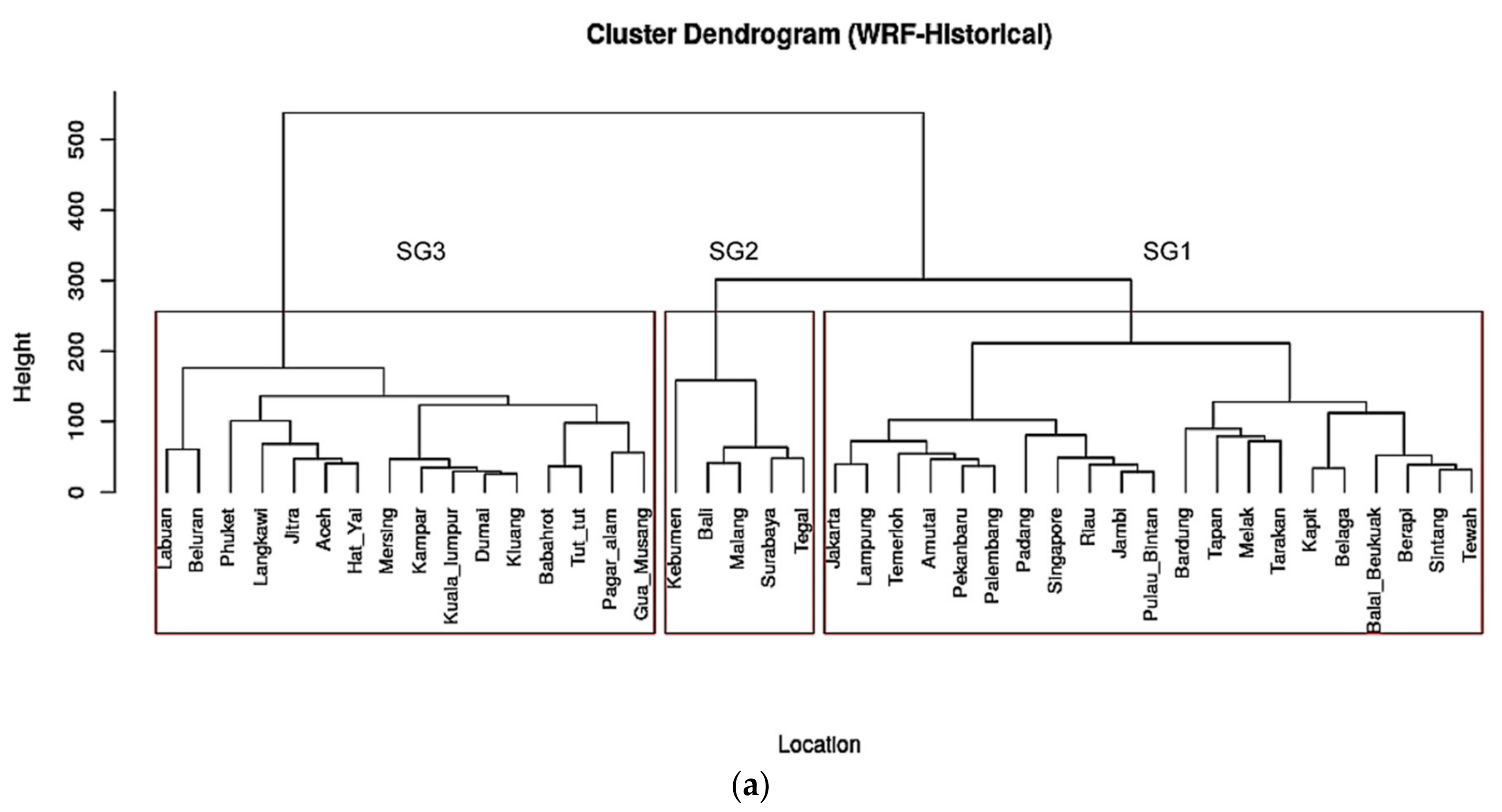
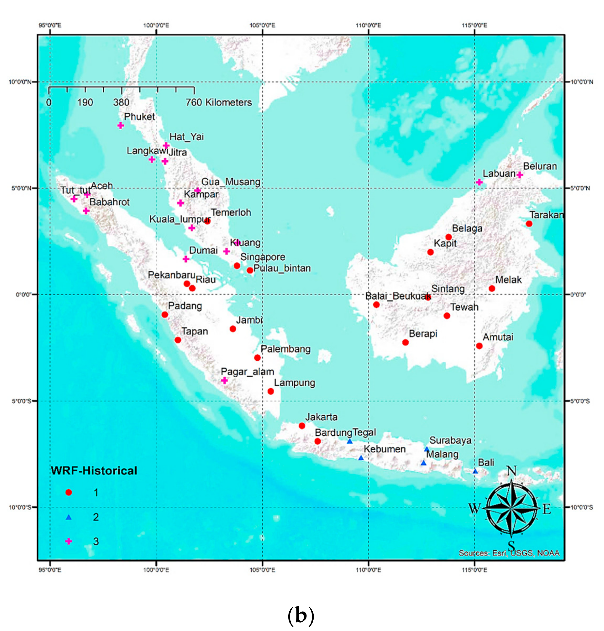
As seen in Figure 7a, three SGs, i.e., SG1, SG2, SG3 were formed from the WRF historical data. SG1 consisted of the highest number (21) of stations, while SG2 had the smallest (5), while SG3 included 16. The distribution of the clusters on a spatial map is shown in Figure 7b. It is observed that the most populated cluster SG1 encompasses most of the grid stations over Borneo. Also, Borneo having the largest tropical rainforest receives more precipitation compared to all other regions in the WMC. Apart from Borneo, SG1 also captured grid stations with similar land-use patterns over Sumatra and Malaysia that were near the Borneo landmass. It was observed that most of the stations within SG1 had similar land-use patterns (see Figure 2b), i.e., rain-forest except for two grids over Java, i.e., Jakarta and Bardung, which have an urban land-use pattern. The possible similarity of these locations with other members of SG1 is the high intensity of precipitation received by this region throughout the year, as they lie on the windward side of mountains (see Figure 2a and Figure 7b).

SG2 consists of five grid locations that lie over the Java landmass (Figure 7). All these lie near the western coast of Java and have an urban land-use pattern. These locations received moderate to heavy precipitation, depending on the season.

Finally, SG3, the second most populated cluster, mostly included grid locations north of the Equator. Most of these stations are in Peninsular Malaysia while the other locations are over Sumatra (see Figure 8). Almost all the locations in SG2 have proximity to the sea. Unlike SG1 and SG2, SG3 experiences maximum precipitation for the SON season.

4.2. Spatial Grouping for RCP 4.5 WRF–CMIP5 Data (2030–2060)

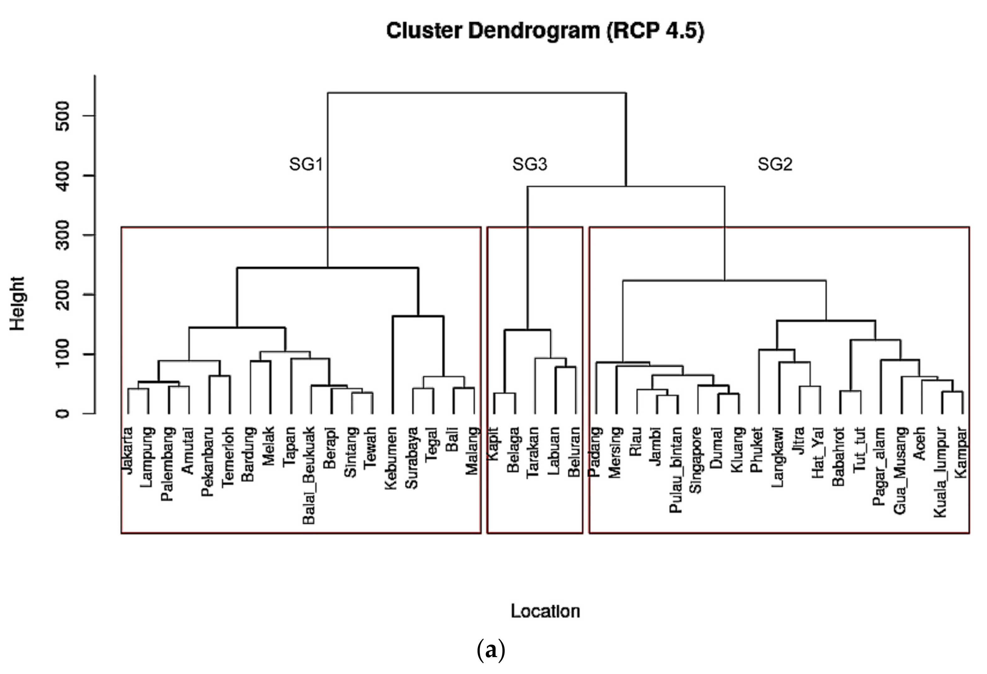
SGs corresponding WRF–CMI5 (RCP 4.5) were observed to be different compared to the historical SGs (see Figure 7 and Figure 8). There were three clusters (see Figure 8a) SG1, SG2, SG3. SG2 was the most populated member with 19 members. However, SG1 had 18 members. SG3 was the least populated member with 5 members.

SG1 for WRF–CMIP5 (RCP 4.5) was similar to SG1 of CHIRPS-25km (historical) regarding the stations captured by this group (see Figure 7 and Figure 8). However, SG1 for WRF–CMIP5 (RCP 4.5) gained more grid locations over Java, bringing the entire island under a single group, whereas within SG1 of WRF (historical) both SG1 and SG2 both share location grids in Java. Furthermore, SG1 for WRF–CMIP5 (RCP 4.5) lost some of its members in Borneo in comparison to SG1 of WRF (historical) that captured all the grid locations over Borneo. The grid locations over Borneo that were occupied by SG1 for the historical time period were now held by SG3 for RCP 4.5, i.e., a new pattern that emerged over the eastern part of Borneo.

SG2 for WRF–CMIP5 (RCP 4.5) was similar to SG3 of the WRF (historical) cluster, as most of the clusters within them were similar to each other. However, it was seen that SG2 of WRF–CMIP5 (RCP 4.5) gained more stations over Sumatra compared to its counterpart SG3 from WRF (historical).

Lastly, SG3, the least populated group, was constrained to the area of eastern Borneo. This group was recognized as a newly formed group in the future over Borneo. The stations within this group mostly included the grid locations that lie near steep terrain and mountains or sea (see Figure 2a).

4.3. Spatial Grouping for RCP 8.5 WRF–CMIP5 Data (2030–2060)

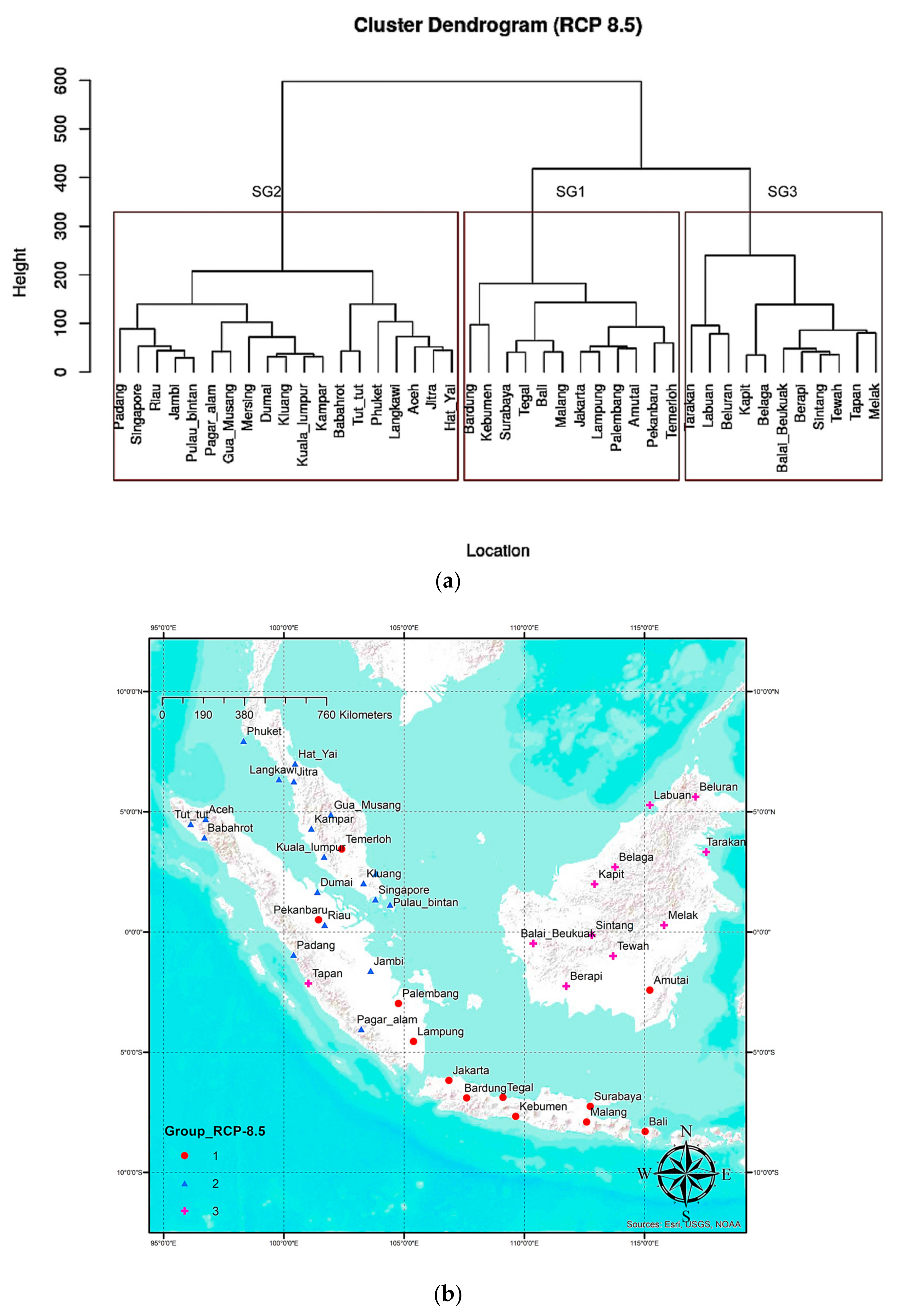
The SGs for WRF–CMIP5 (RCP 8.5) were observed to be very similar to SGs for WRF–CMIP5 (RCP 4.5) for Java, Sumatra, and the Malay Peninsula in terms of the locations occupied by SG1 and SG2 for both the RCPs. However, a significant difference was seen over Borneo (see Figure 8 and Figure 9). While a new pattern for SG3 emerged over eastern Borneo for RCP 4.5, SG3 for RCP 8.5 now almost eliminated the presence of the SG1 group over Borneo, leaving only the Amutai location.

SGs corresponding to WRF–CMI5 (RCP 8.5) were also observed to be different compared to WRF (historical) SGs (see Figure 7 and Figure 9). SG2 was the most populated with 20 stations. SG1 and SG3 both had 11 stations within them.

SG1 for WRF–CMIP5 (RCP 8.5) was similar to SG1 of WRF (historical). However, SG1 for WRF–CMIP5 (RCP 8.5) gained some stations over Java in comparison with SG1 of WRF (historical), making Java more homogeneous and mostly covered by SG1. Furthermore, SG1 for WRF–CMIP5 (RCP 8.5) lost all stations over Borneo except for one, in comparison to SG1 of WRF (historical) that encompassed all the grid stations over Borneo.

SG2 for WRF–CMIP5 (RCP 8.5) over Sumatra was similar to SG3 of the CHIRPS-25km cluster, however SG2 of WRF–CMIP5 (RCP 8.5) gained more stations.

4.4. Temporal Groupings of Historical WRF Data

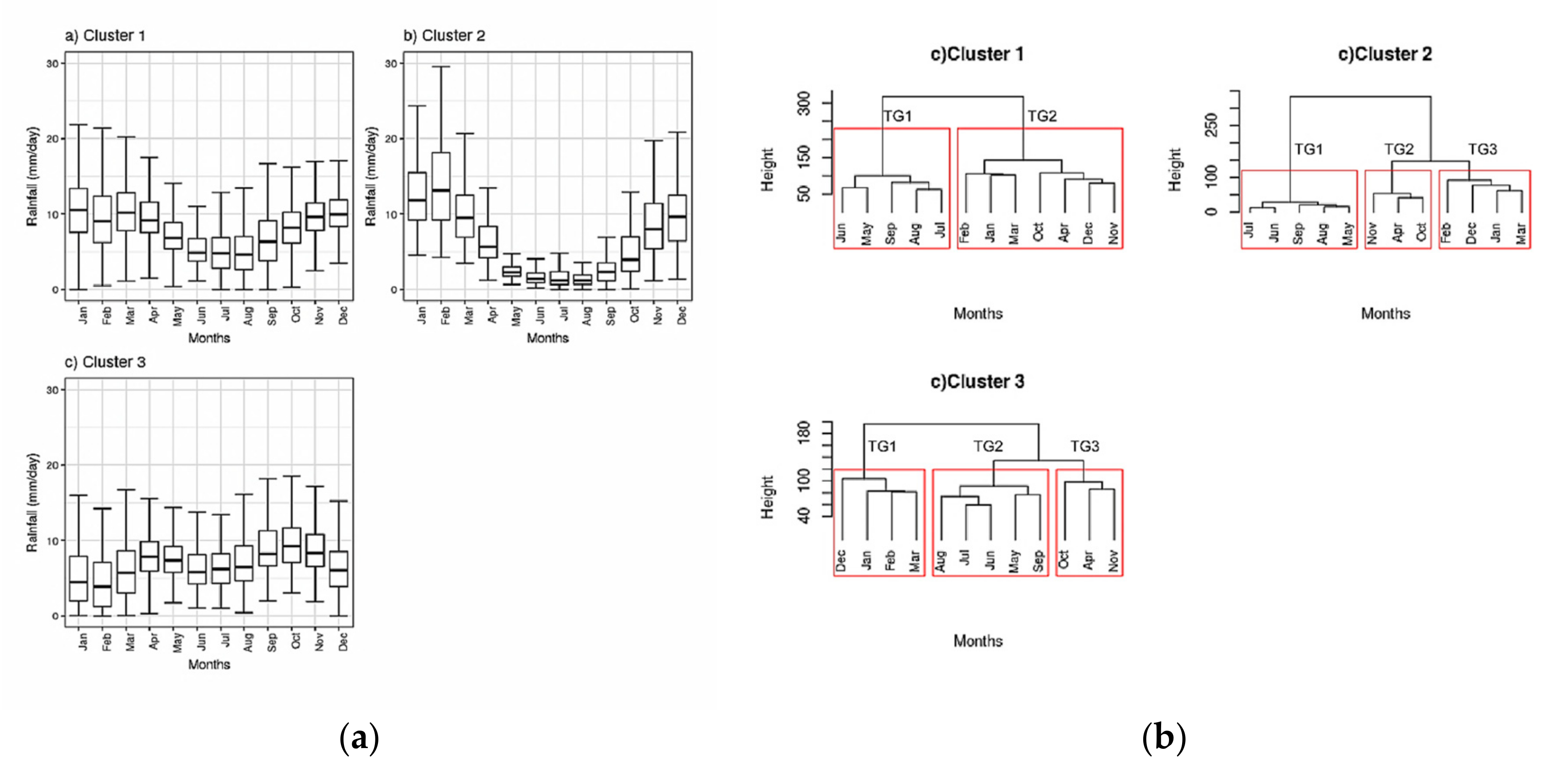
Once the SGs had been discovered, Ward’s CA was next applied to the monthly precipitation data for each SG to find temporal groups (TGs) or seasonality within each SG. Box plots were used to represent the monthly precipitation intensity (mm/h) as seen in Figure 10a. TGs corresponding to each SG are shown in Figure 10b.

4.4.1. Temporal Groups (TGs) for SG1

Two seasons, TG1 and TG2, were predicted for SG1 by Ward’s clustering method (as seen in Figure 10b). TG1 was a dry season, as all the months were observed to have a median precipitation of less than 10 mm/day (see Figure 10a). TG2, on the other hand, was the wet season with a median precipitation of 10 mm/day or more for all the months within TG2.

4.4.2. TGs for SG2

Three temporal clusters were formed within SG2. TG1 depicted a dry season with precipitation intensity of less than 8 mm/day for each month. TG2 was composed of two months, April and November, that were transition months between wet to dry and dry to wet seasons, respectively. Lastly, TG3 depicted the rainy season with precipitation intensities of greater than 8 mm/day over the months within this group.

4.4.3. TGs for SG3

Three TGs were classified for SG3. TG1 was the six months predicted to have a precipitation interquartile range (IQR) of below 10 mm/day. Two of the wettest months for SG1 and SG2, i.e., January and December, were observed to have the lowest median in SG3. Also, the variability in January and December precipitation was found to be largest in SG3 by comparison with other months.

4.5. Temporal Grouping for RCP 4.5 WRF–CMIP5 Data (2030–2060)

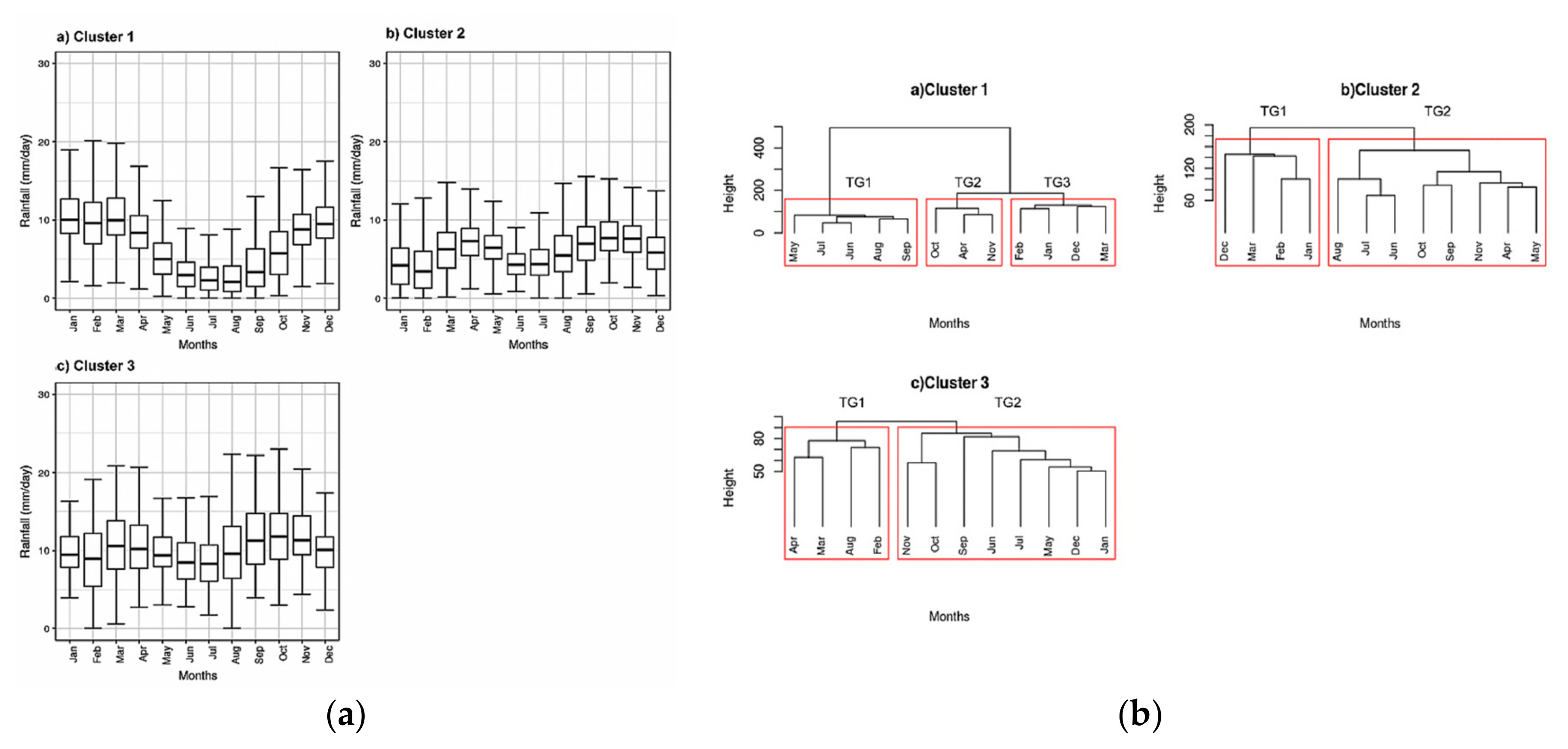
The TGs corresponding to RCP 4.5 WRF–CMIP5 data for all SGs are shown in Figure 11.

4.5.1. TGs for SG1

Three TGs were discovered for SG1. TG1 (as seen in Figure 11) corresponded to the dry season (May–September). TG2 appeared to be discontinuous transition periods between wet and dry months, i.e., March and April, with April as the transition month, and October–November as a transition period from the dry to the rainy season. Finally, TG3 corresponds to the rainy season (DJF) with median precipitation close to 10 mm/day.

4.5.2. TGs for SG2

Two distinct TGs were found for SG2. This SG was comparatively dry with a median below 10 mm/day observed for most of the months (Figure 11b). The classification was based, comparatively, on wet and dry seasons. As seen in Figure 11b, TG1 encompassed the months from December to March while other months were part of TG2.

4.5.3. TGs for SG3

The precipitation for the TGs corresponding to SG3 was uniform and steady (see Figure 11). The two clusters formed for SG2 had very similar characteristics to each other as seen from the box plots; the median and IQR of all the months are approximately consistent. The minimum value for the TG1 cluster was lower compared to the TG2 cluster. Also, all the members of the TG1 cluster had higher variability with a median equal or less to 10 mm/day.

4.6. Temporal Grouping for RCP 8.5 WRF–CMIP5 Data (2030–2060)

The TGs corresponding to RCP 8.5 WRF–CMIP5 data for SGs are shown in Figure 12.

4.6.1. TGs for SG1

As observed from SGs for RCP 4.5 and RCP 8.5 (see Figure 8 and Figure 9), members in SG1 for RCP 4.5 WRF–CMIP5 were similar to SG1 for RCP 8.5 WRF–CMIP5. Then, as expected, three TGs were formed for SG1 (RCP 8.5) as for SG1 (RCP 4.5). Interestingly, as seen in Figure 12a, the monthly precipitation intensity median for SG1 (RCP 8.5) was close to the median for months with SG1 (RCP 4.5).

4.6.2. TGs for SG2

A significant change in the median monthly precipitation and TGs were observed for SG2, corresponding to RCP 4.5 (see Figure 11) and RCP 8.5 (see Figure 12). SG2 for RCP 8.5 was discovered to have four TGs, whereas only two were formed within SG2 for RCP 4.5. TG1 here was created from two of the driest months for SG2, while TG2 appeared to be the transition intervals. TG3 was composed of months that were dry but had smaller IQR (variability) compared to TG1 dry months. Finally, TG4 was a grouping of the wettest months within SG2.

4.6.3. TGs for SG3

SG3 was the most dominant cluster over Borneo, as it grouped most of the locations over the Borneo area. The most significant difference between SGs for RCP 8.5 and SGs RCP 4.5 was because more locations within Borneo were captured by SG3 of RCP 8.5 than by SG3 of RCP 4.5. Although the monthly box plots for SG3 (RCP4.5) and SG3 (RCP 8.5) are similar, the TGs formed were very different. SG3 (RCP 8.5) has three TGs while SG3 (RCP 4.5) had two TGs. TG1 in RCP 8.5 encompassed wet months with a median close to 10 mm/day and large IQR. TG2 had a comparatively lesser IQR compared to TG1, and was composed of wet months. TG3 was the dry season for SG3.

5. Re-Clustering of Precipitation under Representative Concentration Pathway (RCP) Scenarios

Table 2. The distribution of SGs over four landmasses for Historical and future time period (RCP 4.5 and RC.

	Number of SGs (with Minimum than Two Locations in a SG)
Landmass	Historical	RCP 4.5	RCP 8.5
Sumatra	2	2	2
Java	2	1	1
Borneo	1	2	1
Malaysian Peninsula	2	1	1

gives the distribution of SGs over the four major land masses, showing a clear trend in the redistribution of SGs observed in this study. Individual landmasses over the WMC would tend to have a more homogeneous precipitation distribution in the future. Apart from Sumatra, all the landmasses would mostly have a single SG under RCP 8.5. Although Sumatra was consistent with the number of SGs within its spatial boundary, changes in characteristics, i.e., TGs and intensity of monthly precipitation, were observed. Thus, a change in internal as well as overall structure of SGs for monthly precipitation is noted.

Table 3. Distribution of locations among the clusters over the five different landmasses in WMC for monthly precipitation.

Island Landmass	SG1			SG2			SG3			Total Stations per Landmass
	HIS	RCP 4.5	RCP 8.5	HIS	RCP 4.5	RCP 8.5	HIS	RCP 4.5	RCP 8.5
Sumatra	7	4	3	0	8	8	5	0	1	12
Java	2	7	7	5	0	0	0	0	0	7
Malaysia	1	1	1	0	8	8	8	0	0	9
Borneo	9	6	1	0	0	0	2	5	10	11
Ind. Island	2	0	0	0	2	2	0	0	0	2

further shows the distribution of locations among the SGs for each landmass covering historical and future conditions. Borneo, of all the landmasses, experiences the most significant changes when going from RCP 4.5 to RCP 8.5. The distribution of SGs denoted as (SG1, SG2, SG3) over Borneo under historical is (9, 0, 2) which changes to (1, 10, 0) under RCP 8.5. Also, the Borneo stations have almost equal weights between SG1 and SG3 for RCP 4.5 that later amalgamate to SG3 under RCP 8.5. Thus, Borneo becomes highly homogeneous under RCP 8.5 in terms of spatial distribution of monthly precipitation and along with seasonality, i.e., following the TGs of SG3. Similarly, the Malaysian Peninsula has a smaller redistribution, going from (1, 0, 8) under historical to (1, 8, 0) under both RCP 4.5 and RCP 8.5. Lastly, Java also sees a redistribution trend where the SGs change from (2, 5, 0) historical to (7, 0, 0) under RCP 4.5 and RCP 8.5.

6. Conclusions and Recommendations

This paper analyzes the change in the spatial and seasonal patterns of precipitation under climate change. Ward’s clustering method was used to study the redistribution of precipitation at 42 locations over the WMC using WRF–CMIP5 (25 km) output for the years 2030 to 2060. As this was a comparative study, only three SGs were considered that had a height (between cluster distance) of ~300. It was observed that SGs formed for WRF–CMIP5 (RCP 4.5 and RCP 8.5) were very different from historical groupings. The difference between SGs would signify changes in precipitation over the next 25 years. While comparing the SGs for RCP 4.5 and RCP 8.5, it was observed that of all the landmasses, Borneo would see the most significant redistribution of precipitation, being re-clustered to one spatial group along with its temporal groups (i.e., seasonality). Similar but smaller changes in monthly precipitation patterns were also seen for the landmasses of Malaysia and Java.

Future studies can focus on applying clustering analysis on variables such as temperature, wind and relative humidity in order to understand the variables affecting the distribution and redistribution of precipitation over the WMC. Research can also focus on daily and hourly data in order to examine the distribution of daily climatology as well as the diurnal precipitation cycle. Lastly, the redistribution of precipitation should be studied in more detail by using an ensemble of RCMs that examines model uncertainty and has a resolution higher than 25 km.

References

1. Mailhot, A.; Duchesne, S.; Caya, D.; Talbot, G. Assessment of future change in intensity-duration-frequency (IDF) curves for Southern Quebec using the Canadian Regional Climate Model (CRCM). J. Hydrol. 2007, 347, 197–210. [Google Scholar] [CrossRef]
2. Mirhosseini, G.; Srivastava, P.; Stefanova, L. The impact of climate change on rainfall Intensity-Duration-Frequency (IDF) curves in Alabama. Reg. Environ. Chang. 2013, 13, 25–33. [Google Scholar] [CrossRef]
3. Liew, S.C.; Raghavan, S.V.; Liong, S.Y. How to construct future IDF curves, under changing climate, for sites with scarce rainfall records? Hydrol. Process. 2014, 28, 3276–3287. [Google Scholar] [CrossRef]
4. Shrestha, A.; Babel, M.S.; Weesakul, S.; Vojinovic, Z. Developing Intensity–Duration–Frequency (IDF) Curves under Climate Change Uncertainty: The Case of Bangkok, Thailand. Water 2017, 9, 145. [Google Scholar] [CrossRef]
5. Olayide, O.E.; Tetteh, I.K.; Popoola, L. Differential impacts of rainfall and irrigation on agricultural production in Nigeria: Any lessons for climate-smart agriculture? Agric. Water Manag. 2016, 178, 30–36. [Google Scholar] [CrossRef]
6. Misra, A.K. Climate change and challenges of water and food security. Int. J. Sustain. Built Environ. 2014, 3, 153–165. [Google Scholar] [CrossRef]
7. Zhang, Q.; Gemmer, M.; Chen, J. Climate changes and flood/drought risk in the Yangtze Delta, China, during the past millennium. Quat. Int. 2008, 176, 62–69. [Google Scholar] [CrossRef]
8. Wilhite, D.A.; Sivakumar, M.V.; Pulwarty, R. Managing drought risk in a changing climate: The role of national drought policy. Weather Clim. Extremes 2014, 3, 4–13. [Google Scholar] [CrossRef]
9. Berga, L.; Buil, J.; Bofill, E.; De Cea, J.; Perez, J.G.; Mañueco, G.; Polimon, J.; Soriano, A.; Yagüe, J. Dams and Reservoirs, Societies and Environment in the 21st Century, Two Volume Set: Proceedings of the International Symposium on Dams in the Societies of the 21st Century, 22nd International Congress on Large Dams (ICOLD), Barcelona, Spain, 18 June 2006; CRC Press: Boca Raton, FL, USA, 2006. [Google Scholar]
10. Ledec, G.; Quintero, J.D. Good Dams and Bad Dams: Environmental Criteria for Site Selection of Hydroelectric Projects; Latin America and Caribbean Region Sustainable Development Working Paper Series; World Bank: Washington, DC, USA, 2003. [Google Scholar]
11. Han, B.-P.; Liu, Z. Tropical and Sub-Tropical Reservoir Limnology in China: Theory and Practice; Springer Science & Business Media: Berlin, Germany, 2011; Volume 91. [Google Scholar]
12. Bates, B. Climate Change and Water: IPCC Technical Paper VI; World Health Organization: Geneva, Switzerland, 2009. [Google Scholar]
13. Donat, M.G.; Lowry, A.L.; Alexander, L.V.; O’Gorman, P.A.; Maher, N. More extreme precipitation in the world’s dry and wet regions. Nat. Clim. Chang. 2016, 6, 508–513. [Google Scholar] [CrossRef]
14. Schoof, J.T.; Robeson, S.M. Projecting changes in regional temperature and precipitation extremes in the United States. Weather Clim. Extremes 2016, 11, 28–40. [Google Scholar] [CrossRef]
15. Rotstayn, L.D.; Ryan, B.F.; Penner, J.E. Precipitation changes in a GCM resulting from the indirect effects of anthropogenic aerosols. Geophys. Res. Lett. 2000, 27, 3045–3048. [Google Scholar] [CrossRef]
16. Sharma, D.; Gupta, A.D.; Babel, M. Spatial disaggregation of bias-corrected GCM precipitation for improved hydrologic simulation: Ping River Basin, Thailand. Hydrol. Earth Syst. Sci. Discuss. 2007, 11, 1373–1390. [Google Scholar] [CrossRef]
17. Turco, M.; Llasat, M.C.; Herrera, S.; Gutiérrez, J.M. Bias correction and downscaling of future RCM precipitation projections using a MOS-Analog technique. J. Geophys. Res.Atmos. 2017, 122, 2631–2648. [Google Scholar] [CrossRef]
18. Trenberth, K.E. Changes in precipitation with climate change. Clim. Res. 2011, 47, 123–138. [Google Scholar] [CrossRef]
19. Intergovernmental Panel on Climate Change. Climate Change 2014–Impacts, Adaptation and Vulnerability: Regional Aspects; Cambridge University Press: Cambridge, UK, 2014. [Google Scholar]
20. Chang, C.-P. East Asian Monsoon; World Scientific: Singapore, 2004; Volume 2. [Google Scholar]
21. Neale, R.; Slingo, J. The maritime continent and its role in the global climate: A GCM study. J. Clim. 2003, 16, 834–848. [Google Scholar] [CrossRef]
22. Qian, J.-H. Why precipitation is mostly concentrated over islands in the Maritime Continent. J. Atmos. Sci. 2008, 65, 1428–1441. [Google Scholar] [CrossRef]
23. Murtagh, F.; Legendre, P. Ward’s hierarchical agglomerative clustering method: Which algorithms implement Ward’s criterion? J. Classif. 2014, 31, 274–295. [Google Scholar] [CrossRef]
24. Ward, J.H., Jr. Hierarchical grouping to optimize an objective function. J. Am. Stat. Assoc. 1963, 58, 236–244. [Google Scholar] [CrossRef]
25. Teo, C.-K.; Koh, T.-Y.; Chun-Fung Lo, J.; Bhatt, B.C. Principal component analysis of observed and modeled diurnal rainfall in the Maritime Continent. J. Clim. 2011, 24, 4662–4675. [Google Scholar] [CrossRef]
26. Rao, A.; Hsieh, C. Empirical orthogonal function analysis of rainfall and runoff series. Water Resour. Manag. 1991, 4, 235–250. [Google Scholar] [CrossRef]
27. Rajagopalan, B.; Lall, U. A k-nearest-neighbor simulator for daily precipitation and other weather variables. Water Resour. Res. 1999, 35, 3089–3101. [Google Scholar] [CrossRef]
28. Ben-Hur, A.; Guyon, I. Detecting stable clusters using principal component analysis. Funct. Genom.: Methods Protoc. 2003, 159–182. [Google Scholar]
29. Steinbach, M.; Karypis, G.; Kumar, V. A Comparison of Document Clustering Techniques. In Proceedings of the KDD Workshop on Text Mining, Boston, MA, USA, 20–23 August 2000; pp. 525–526. [Google Scholar]
30. Johnson, S.C. Hierarchical clustering schemes. Psychometrika 1967, 32, 241–254. [Google Scholar] [CrossRef] [PubMed]
31. Zhao, Y.; Karypis, G. Evaluation of hierarchical clustering algorithms for document datasets. In Proceedings of the eleventh international conference on Information and knowledge management, McLean, VA, USA, 4–9 November 2002; pp. 515–524. [Google Scholar]
32. Taguchi, Y.; Iwadate, M.; Umeyama, H. Principal component analysis-based unsupervised feature extraction applied to in silico drug discovery for posttraumatic stress disorder-mediated heart disease. BMC Bioinform. 2015, 16, 139. [Google Scholar] [CrossRef] [PubMed]
33. Blashfield, R.K. Mixture model tests of cluster analysis: Accuracy of four agglomerative hierarchical methods. Psychol. Bull. 1976, 83, 377. [Google Scholar] [CrossRef]
34. Varikoden, H.; Samah, A.; Babu, C. Spatial and temporal characteristics of rain intensity in the peninsular Malaysia using TRMM rain rate. J. Hydrol. 2010, 387, 312–319. [Google Scholar] [CrossRef]
35. Suhaila, J.; Jemain, A.A.; Hamdan, M.F.; Zin, W.Z. Comparing rainfall patterns between regions in Peninsular Malaysia via a functional data analysis technique. J. Hydrol. 2011, 411, 197–206. [Google Scholar] [CrossRef]
36. Manton, M.; Della-Marta, P.; Haylock, M.; Hennessy, K.; Nicholls, N.; Chambers, L.; Collins, D.; Daw, G.; Finet, A.; Gunawan, D. Trends in extreme daily rainfall and temperature in Southeast Asia and the South Pacific: 1961–1998. Int. J. Climatol. 2001, 21, 269–284. [Google Scholar] [CrossRef]
37. BMKG, Badan Meteorologi, Klimatologi, dan Geofisika. 2017. Available online: http://www.bmkg.go.id/ (accessed on 24 August 2017).
38. Ramage, C.S. Role of a Tropical “Maritime Continent” in the Atmospheric Circulation. Mon. Weather Rev. 1968, 96, 365–370. [Google Scholar] [CrossRef]
39. Intergovernmental Panel on Climate Change (IPCC). Climate Change 2013: The Physical Science Basis. Contribution of Working Group I to the Fifth Assessment Report of the Intergovernmental Panel on Climate Change; Stocker, T.F., Qin, D., Plattner, G.-K., Tignor, M., Allen, S.K., Boschung, J., Nauels, A., Xia, Y., Bex, V., Midgley, P.M., Eds.; Cambridge University Press: Cambridge, UK; New York, NY, USA, 2013; p. 1535. [Google Scholar]
40. Intergovernmental Panel on Climate Change (IPCC). Summary for Policymakers. In Climate Change 2013: The Physical Science Basis. Contribution of Working Group I to the Fifth Assessment Report of the Intergovernmental Panel on Climate Change; Stocker, T.F., Qin, D., Plattner, G.-K., Tignor, M., Allen, S.K., Boschung, J., Nauels, A., Xia, Y., Bex, V., Midgley, P.M., Eds.; Cambridge University Press: Cambridge, UK; New York, NY, USA, 2013; pp. 1–30. [Google Scholar]
41. Funk, C.; Peterson, P.; Landsfeld, M.; Pedreros, D.; Verdin, J.; Shukla, S.; Husak, G.; Rowland, J.; Harrison, L.; Hoell, A. The climate hazards infrared precipitation with stations—A new environmental record for monitoring extremes. Sci. Data 2015, 2. [Google Scholar] [CrossRef] [PubMed]
42. Thompson, G.; Field, P.R.; Rasmussen, R.M.; Hall, W.D. Explicit forecasts of winter precipitation using an improved bulk microphysics scheme. Part II: Implementation of a new snow parameterization. Mon. Weather Rev. 2008, 136, 5095–5115. [Google Scholar] [CrossRef]
43. Iacono, M.J.; Delamere, J.S.; Mlawer, E.J.; Shephard, M.W.; Clough, S.A.; Collins, W.D. Radiative forcing by long-lived greenhouse gases: Calculations with the AER radiative transfer models. J. Geophys. Res. Atmos. 2008, 113. [Google Scholar] [CrossRef]
44. Hong, S.-Y.; Noh, Y.; Dudhia, J. A new vertical diffusion package with an explicit treatment of entrainment processes. Mont. Weather Rev. 2006, 134, 2318–2341. [Google Scholar] [CrossRef]
45. Tewari, M.; Chen, F.; Wang, W.; Dudhia, J.; LeMone, M.; Mitchell, K.; Ek, M.; Gayno, G.; Wegiel, J.; Cuenca, R. Implementation and Verification of the Unified NOAH Land Surface Model in the WRF Model. In Proceedings of the 20th Conference on Weather Analysis and Forecasting/16th Conference on Numerical Weather Prediction, Seattle, WA, USA, 11 January 2004. [Google Scholar]
46. Zhang, C.; Wang, Y.; Hamilton, K. Improved representation of boundary layer clouds over the southeast Pacific in ARW-WRF using a modified Tiedtke cumulus parameterization scheme. Mon. Weather Rev. 2011, 139, 3489–3513. [Google Scholar] [CrossRef]
47. Piani, C.; Haerter, J.; Coppola, E. Statistical bias correction for daily precipitation in regional climate models over Europe. Theor. Appl. Climatol. 2010, 99, 187–192. [Google Scholar] [CrossRef]
48. Wilks, D.S. Statistical Methods in the Atmospheric Sciences; Academic Press: Cambridge, MA, USA, 2011; Volume 100. [Google Scholar]
49. Katz, R. Extreme value theory for precipitation: Sensitivity analysis for climate change. Adv. Water Resour. 1999, 23, 133–139. [Google Scholar] [CrossRef]
50. Husak, G.J.; Michaelsen, J.; Funk, C. Use of the gamma distribution to represent monthly rainfall in Africa for drought monitoring applications. Int. J. Climatol. 2007, 27, 935–944. [Google Scholar] [CrossRef]
51. Al-Suhili, R.H.; Khanbilvardi, R. Frequency analysis of the monthly rainfall data at Sulaimania Region, Iraq. Am. J. Eng. Res. 2014, 3, 212–222. [Google Scholar]
52. Wilcke, R.A.I.; Mendlik, T.; Gobiet, A. Multi-variable error correction of regional climate models. Clim. Chang. 2013, 120, 871–887. [Google Scholar] [CrossRef]
53. Amengual, A.; Homa, V.; Romero, R.; Alonso, S.; Ramis, C. A statistical adjustment of regional climate model outputs to local scales: Application to Platja de Palma, Spain. J. Clim. 2012, 25, 939–957. [Google Scholar] [CrossRef]
54. Gutjahr, O.; Heinemann, G. Comparing precipitation bias correction methods for high-resolution regional climate simulations using COSMO-CLM. Theor. Appl. Climatol. 2013, 114, 511–529. [Google Scholar] [CrossRef]
55. The R Stats Package. 2017. Available online: https://stat.ethz.ch/R-manual/R-devel/library/stats/html/00Index.html (accessed on 24 August 2017).
56. Lehmann, J.; Coumou, D.; Frieler, K. Increased record-breaking precipitation events under global warming. Clim. Chang. 2015, 132, 501–515. [Google Scholar] [CrossRef]
Figure 1. A flowchart showing the clustering framework used in this study.
Climate 05 00084 g001
Figure 2. Spatial map showing 42 locations and (a) topography, and (b) land-use patterns of the study region.
Climate 05 00084 g002
Figure 3. WRF physics parameterization used for running the Coupled Model Intercomparison Project Phase 5 (CMIP5) model.
Climate 05 00084 g003
Figure 4. Comparison plots for the seasonal precipitation rate (mm/day) between 5 km CHIRPS (left) and 25 km WRF (right) for the baseline period (1980–2005).
Climate 05 00084 g004
Figure 5. Percentage bias in precipitation rate (left) and the corresponding bias over the maximum spatial rain rate (right) plots of the seasonal precipitation rate (mm/day) between weather research and forecasting (WRF) historical (1980–2005) and CHIRPS (bi-linearly averaged to 25 km) as observed data.
Climate 05 00084 g005
Figure 6. Percentage precipitation changes (future modeled precipitation—historical modeled precipitation)/(historical modeled precipitation) for WRF model RCP 4.5 (left) and RCP 8.5 (right) for the years 2030–2060.
Climate 05 00084 g006
Figure 7. Cluster analysis groups (SG1–SG3) for WRF- historical (25 km) data for the 41 stations: (a) dendrograms based on their spatial similarity; and (b) spatial representation of the clusters on a map.
Climate 05 00084 g007aClimate 05 00084 g007b
Figure 8. Cluster analysis groups (SG1–SG3) for RCP 4.5: (a) dendrograms based on their spatial similarity; and (b) SG representation on a map.
Climate 05 00084 g008aClimate 05 00084 g008b
Figure 9. Cluster analysis groups (SG1–SG3) for RCP 8.5: (a) dendrograms based on their spatial similarity; and (b) spatial representation of the clusters on a map.
Climate 05 00084 g009
Figure 10. (a) The box plots and (b) dendrograms of TGs for the three different SGs discovered in the historical WRF data.
Climate 05 00084 g010
Figure 11. (a) The box plots and (b) dendrograms of TGs for the three SGs discovered in the WRF–CMIP5 (RCP 4.5).
Climate 05 00084 g011
Figure 12. (a) The box plots and (b) dendrograms of TGs for the three different SGs discovered in the WRF–CMIP5 (RCP 8.5).
Climate 05 00084 g012