Impacts of Solar Radiation Modification on Extreme Climate Indices in the Philippines

Abstract

The rising global temperature and changing climate patterns have increased the frequency and intensity of extreme heat events, droughts, and heavy precipitation, significantly affecting agriculture, water resources, and ecosystems. Solar radiation management (SRM) has been proposed as a geoengineering strategy to mitigate these effects by reducing incoming solar radiation. This study evaluated future trends and variability in rainfall and temperature extremes in the Philippines under GeoMIP (G6Solar and G6Sulfur) and ScenarioMIP (SSP2-4.5 and SSP5-8.5) projections. Using five General Circulation Models (GCMs) and a suite of 10 climate indices recommended by the Expert Team on Climate Change Detection and Indices (ETCCDI), changes in extreme precipitation and temperature across different climate zones in the Philippines were assessed. Climate projections for the future (2041–2070) scenario were analyzed using bias correction, downscaling, and spatial interpolation techniques. Trend analysis was evaluated using the Mann–Kendall test and Sen’s slope estimator, while variability was assessed through statistical methods. The results show widespread warming and increased extreme precipitation, but these trends vary significantly across regions. Non-uniform responses emerge across scenarios, with some northern regions experiencing decreases in specific precipitation indices despite the broader warming trend under SRM and non-SRM conditions. These findings provide critical insights into the potential impacts of SRM on future climate extremes in the Philippines and guidance on climate policy recommendations for decision-makers and stakeholders.

1. Introduction

The need to examine the impacts of climate change has become increasingly important due to rising global temperatures and altered climatic patterns [1]. Extreme heat events have notably increased in scale, intensity, frequency, and duration, coinciding with rising average global temperatures, suggesting that simultaneous heatwaves and droughts have likely become more frequent globally over the past century due to human activities [2]. Studies suggest significant increases in waterlogging, salinity, carbon uptake, soil erosion, food insecurity, and rainfall, which contribute to declines in agricultural productivity and crop yields [3,4,5,6]. In response to the need to mitigate these effects, there has been growing interest in the potential applications of geoengineering, in which atmospheric processes are intentionally manipulated [7]. Efforts in limiting global warming to 1.5 °C above pre-industrial levels have intensified since the Paris Agreement in 2015. Still, current mitigation strategies remain insufficient, prompting consideration of solar radiation management (SRM) as a possible supplementary approach [8,9].

SRM can potentially cool the Earth’s surface by decreasing the amount of incoming solar radiation absorbed or reflected [10]. This climate intervention technology aims to reduce the impacts of climate change by managing solar radiation levels, and further affects temperature and precipitation. Early climate modeling studies have evolved from idealized global solar dimming scenarios to more policy-relevant experiments involving stratospheric aerosol injection (SAI) to highlight complex regional climate responses [11,12]. These localized impacts are significant, especially for areas with heightened risks of temperature extremes, precipitation variability, and hydrological changes, such as countries in the Global South [13]. In the Philippines, there is a limited understanding of how SRM, particularly SAI and solar dimming, affects local climate variables such as temperature, precipitation, and extreme weather events [6,12].

Despite advances in global climate modeling, knowledge gaps persist regarding the heterogeneity of SRM effects at country-level scales, including potential trade-offs like altered monsoon patterns or drought exacerbation [14,15,16]. Several studies have assessed the efficacy and risks of SRM, albeit with varied results: some studies emphasize its potential to moderate warming and climate hazards, while others caution about unintended ecological and societal consequences [17,18]. Multi-model intercomparison projects enhance the understanding of uncertainties and model sensitivities, fostering improved experimental design and evaluation frameworks [19,20,21]. However, many studies still rely on idealized or uniform solar reduction scenarios that may not fully capture the complexity of real-world deployment strategies or regional heterogeneity [12,22]. The lack of standardized protocols for scenario selection and performance assessment impedes comparability and decision-making relevance [11,14,19].

Given the uncertainties and potential for unintended consequences, multiple studies suggest that SRM should be integrated cautiously as a complementary strategy alongside aggressive greenhouse gas mitigation and adaptation measures rather than as a standalone solution. This integrated approach aligns with the sustainable development goals and climate justice considerations [23,24]. Still, some studies use short simulation periods or limited spatial domains, which limits the understanding of long-term and broader transboundary impacts [25]. Additionally, only few studies thoroughly assess SRM impacts on extreme weather events and their ecological or societal consequences [13].

To address these gaps, this study evaluates the trends and variability in rainfall and temperature extremes in the Philippines under GeoMIP (G6Solar and G6Sulfur) and ScenarioMIP (SSP2-4.5 and SSP5-8.5) scenarios. The study determined future changes in extreme rainfall and temperature using indices relevant to the Expert Team on Climate Change Detection and Indices (ETCCDI) to provide a fundamental analysis of the effects of SRM on extreme climate in the Philippines. The study also analyzed spatio-temporal changes (past versus future) in extreme index trends across the Philippines.

2. Materials and Methods

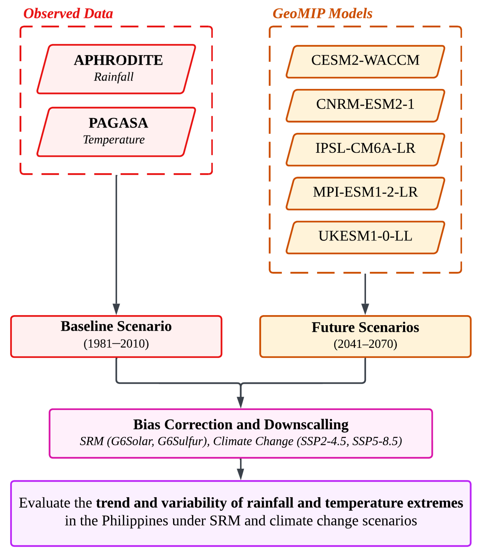
Evaluating changes in rainfall and temperature extremes in the Philippines under different scenarios involves collection of observed, reanalysis, and CMIP6 data for rainfall and temperature prior to bias correction and downscaling, as detailed in Figure 1. Observed rainfall and temperature data were obtained from APHRODITE (Asian Precipitation—Highly Resolved Observational Data Integration Towards Evaluation of Water Resources) and PAGASA (Philippine Atmospheric, Geophysical and Astronomical Services Administration), respectively, while future scenarios were obtained from the first complete ensemble of the 5 Global Climate Models (GCMs) under Coupled Model Intercomparison Project Phase 6 (CMIP6). Climate projections were simulated using GeoMIP and ScenarioMIP for future scenarios (2041–2070). To refine these projections, a 3-step bias correction [26] and additive linear scaling were adopted and applied to rainfall and temperature data, respectively. Nearest-neighbor interpolation was applied to re-grid the climate data to preserve the original statistical distribution of the post-processed data. This method retains the precise magnitude of extreme weather events and discrete physical boundaries by assigning the exact value of the closest station point to the surrounding grid cells [27,28], ensuring that the final spatial visualization directly reflects the original outputs of the localized bias correction algorithms rather than artificial spatial gradients and interpolated numerical artifacts [29]. To evaluate climate index trends, the Mann–Kendall test and Sen’s slope (SS) were used for behavior and magnitude, respectively.

2.1. Study Area

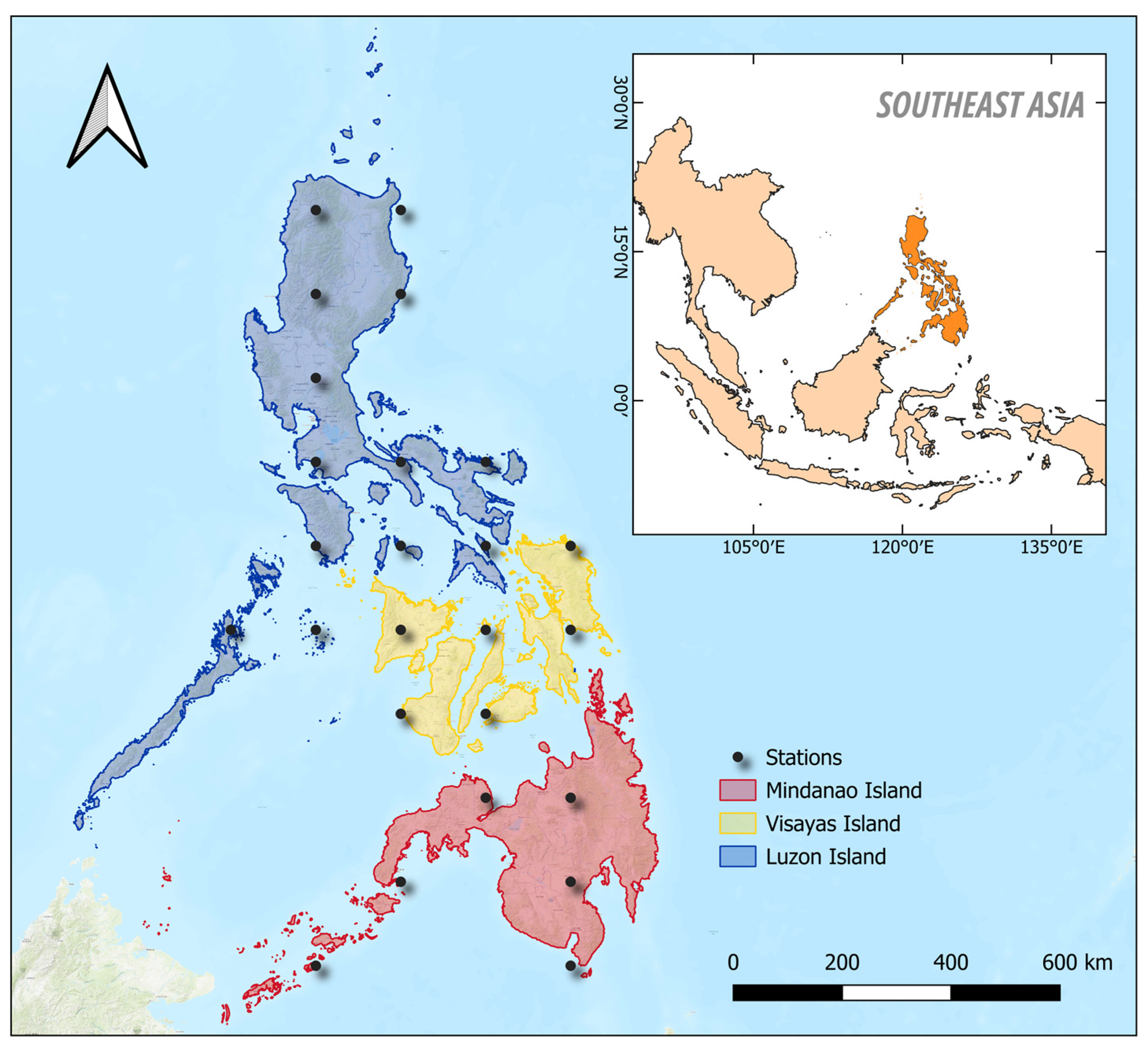
The Philippines is located in Southeast Asia between 4°23′ N and 21°25′ N latitude and 112° E and 127° E longitude (Figure 2) [30,31,32]. The Philippines’ climate is classified as tropical maritime, characterized by generally high temperatures and heavy rainfall with two pronounced seasons: the rainy season (from June to November) and the dry season (from December to May). The country also experiences varied rainfall patterns, as influenced by its location in Southeast Asia. Rainfall distribution on the west coast is influenced by the seasonal monsoon, creating distinct seasonal variations, while areas on the eastern seaboard lack a prominent dry season and experience year-round rainfall due to the northeast monsoon and frequent tropical cyclones. Inland and transitional sub-national regions experience less pronounced seasonal variation, as they are less influenced by monsoons but still experience seasonal shifts in rainfall. However, evenly distributed rainfall throughout the year is observed in equatorial-maritime zones and lowland areas, resulting in consistent moisture availability and making these regions suitable for year-round agriculture.

Geographically, the Philippines is grouped into 3 main island clusters: Luzon includes the northern portion, Visayas includes the central islands, and Mindanao includes the sub-national regions in the south. Politically, the country is further subdivided into 18 sub-national regions and 82 provinces. The data points were based on the 25 grid centroids of APHRODITE established at a 1.40-degree resolution located within or near a landmass in the Philippines.

2.2. Datasets

Climate projections from five GCMs (CESM2-WACCM6, CNRM-ESM2-1, IPSL-CM6A-LR, MPI-ESM1-2-LR, and UKESM1-0-LL) of the Coupled Model Intercomparison Project Phase 6 (CMIP6), archived in the World Climate Research Programme (WCRP), were used for simulations of past and future climate change, and SRM scenarios were obtained from selected experiments of the Geoengineering Model Intercomparison Project (GeoMIP) and Scenario Model Intercomparison Project (ScenarioMIP) for scenarios under SRM and climate change, respectively.

This study considered 1981–2010 as the baseline period and 2041–2070 as the future scenario period. A 30-year reference period was adopted to identify climate conditions in accordance with WMO guidelines for Climatological Standard Normals (CLINOs) [33,34]. Daily gridded datasets for observed precipitation and temperature data were acquired from the Data Integration and Analysis System (DIAS) platform [35]. To perform bias correction to future projections of precipitation and temperature in the selected GCMs, the APHRODITE and PAGASA datasets were obtained. Different bias correction methods were applied to each meteorological parameter, as shown in

Table 1. Temperature and precipitation parameters and the corresponding bias correction methods used.

Variable	Parameter	Baseline Dataset	Bias Correction Method
pr	Precipitation	APHRODITE	3-step
tasmax	Maximum Temperature	PAGASA	Linear
tasmin	Minimum Temperature	PAGASA	Linear

.

APHRODITE is a long-term gridded dataset with data available from 1951 onwards at a 0.5° × 0.5° or 0.25° × 0.25° resolution based on a dense network of rain gauges placed across Asia, including the Himalayas, South and Southeast Asia, and mountainous areas in the Middle East [36]. Studies suggest that use of APHRODITE to measure extreme precipitation underestimates magnitude and overestimates the total number of events [37,38,39]. However, Jaspe-Santander and Tabañag [40] found that APHRODITE could serve as an alternative to observational data and could be suitable for hydrological modeling. It was also found that the APHRODITE dataset, downscaled to a higher resolution of at least 12.5 km, simulated monthly rainfall that was closest to the observation data [41]. A study by Peralta et al. [42] further supports use of APHRODITE (v1101) as it produces fewer statistical errors than other gridded datasets considered (i.e., APHRODITE v1101, CHIRPSv2, TRMM 3B42v7, and PERSIAN-CDR) more suitable for climatological analysis of long-term trends due to its better temporal range.

The PAGASA data obtained for the study include daily observations from 58 synoptic stations distributed across the country. Since these synoptic stations are not well distributed across the study areas, the temperature data were interpolated using Inverse Distance Weighting (IDW) from selected station coordinates. Spatial interpolation was performed using a standard power parameter of 2 to represent quadratic spatial decay, thereby preserving localized station gradients [43]. This configuration balances localized detail with regional trends, preventing spatial discontinuities while avoiding excessive smoothing due to lower weights [44]. Daily temperature and rainfall data were bias-corrected and downscaled before interpolation to obtain re-gridded station data for the future scenario (2041–2070). Only the first complete ensemble for each GCM and experiment was selected for climatological normal analysis to ensure consistency (see

Table 2. Precipitation and temperature data ensemble.

Parameter	GCM	Historical	Climate Change Scenarios		SRM Scenarios
			SSP2-4.5	SSP5-8.5	G6Solar	G6Sulfur
Precipitation (pr)	CESM2-WACCM6	r1i1p1f1	r1i1p1f1	r1i1p1f1	r1i1p1f1	r2i1p1f2 b
	CNRM-ESM2-1	r1i1p1f2	r1i1p1f2	r1i1p1f2	r1i1p1f2	r1i1p1f2
	IPSL-CM6A-LR	r1i1p1f1	r1i1p1f1	r1i1p1f1	r1i1p1f1	r1i1p1f1
	MPI-ESM1-2-LR	r1i1p1f1	r1i1p1f1	r1i1p1f1	r2i1p1f1 a	r2i1p1f1 a
	UKESM1-0-LL	r1i1p1f2	r1i1p1f2	r1i1p1f2	r1i1p1f2	r1i1p1f2
Temperature (tasmin, tasmax)	CESM2-WACCM6	BWHIST c	r2i1p1f1 d	r3i1p1f1 e	r1i1p1f1	r2i1p1f2
	CNRM-ESM2-1	r1i1p1f2	r1i1p1f2	r1i1p1f2	r1i1p1f2	r1i1p1f2
	IPSL-CM6A-LR	r1i1p1f1	r1i1p1f1	r1i1p1f1	r1i1p1f1	r1i1p1f1
	MPI-ESM1-2-LR	r1i1p1f1	r1i1p1f1	r1i1p1f1	r2i1p1f1	r2i1p1f1
	UKESM1-0-LL	r1i1p1f2	r1i1p1f2	r1i1p1f2	r1i1p1f2	r1i1p1f2

^a r1i1p1f1 output only runs until 2099; ^b r1i1p1f1 output has 3 missing days in 2060–2070 NetCDF file; ^c ARISE BWHIST was used due to unavailability of tasmin/tasmax historical data in ESGF node; ^d no r1i1p1f1 output in ESGF node; ^e r1i1p1f1 runs from 2100 to 2200 and no r2i1p1f1 output in ESGF node.

). The same ensembles were obtained for precipitation (pr), minimum temperature (tasmin), and maximum temperature (tasmax) across most GCMs.

While CESM2 provides robust historical simulations overall, due to model configuration errors, only a tiny subset of correct daily tasmin and tasmax variables was available within the Earth System Grid Federation (ESGF) nodes for the historical run [45]. To address this constraint, the study used the continuous ARISE-SAI historical ensemble stream (BWHIST) to conduct baseline historical experiments with the CESM2-WACCM6 model. The use of this ensemble also ensures that the localized baseline temperature extremes provide a robust, forced climate signal with a 10-member ensemble pathway [46]. The presence of data node gaps required replacing realization r3i1p1f1 with the SSP5-8.5 projection and r2i1p1f1 with the SSP2-4.5 timeline. All chosen realization members for the study share identical grid resolutions, fundamental core atmospheric chemistry modules, and physics parameterizations. The transition from the f1 forcing configuration to the f2 forcing index within the G6Sulfur experiment reflects a structural requirement within the GeoMIP6 protocols to implement explicit stratospheric aerosol injection fields in CESM2-WACCM6 accurately [47].

To ensure coherence in GCMs date format, Gregorian calendar was employed to all GCMs to account for leap years and months with 31 days. Linear interpolation was facilitated to ensure data gaps or missing values for the future dataset. Data stations’ locations irregularities were addressed by interpolating using IDW at 0.05-degree resolution.

To map coarse-resolution GeoMIP grid data directly to localized station coordinates, nearest-neighbor extraction was applied. Alternative continuous blending mechanisms, such as bilinear interpolation, fail to accommodate the highly fragmented archipelagic geography of the Philippines [48]. Coarse GCM grid cells routinely bisect contrasting marine environments and steep mountainous terrain. Thus, spatial smoothing introduces severe spatial representativeness errors. Nearest-neighbor extraction effectively eliminates oceanic data irregularity at coastal stations, retaining the discrete, unaveraged extreme thresholds necessary for rigorous localized impact modeling [36,37].

2.3. Bias Correction and Downscaling

Different statistical downscaling techniques were used to transform the coarse-resolution temperature and precipitation data into a fine-resolution dataset accounting for their natural behavior. Temperature acts as a continuous, spatially smooth, and normally distributed variable, heavily influenced by local topography and elevation lapse rates. GCMs tend to simplify these microclimates for coarser resolutions, which overlook complex mountain and valley features [49,50,51]. To manage this, the delta downscaling method was used to account the for the difference between the GCM simulated and historical temperature values. Precipitation, on the other hand, is a highly skewed, zero-inflated, and intermittent variable, characterized by many dry days and occasional, non-linear storm events. GCMs are also known to underestimate rainfall, leading to the ‘drizzle effect,’ where models produce too many low-intensity rainy days and miss heavy, localized storms [26,52,53]. Since a simple delta method is insufficient to correct these distribution issues, a comprehensive 3-step bias correction was applied for precipitation.

The 3-step bias correction improves estimates of local precipitation from the selected GCMs. Daily precipitation records extracted from the APHRODITE dataset were used as an observational baseline reference for bias correction. Instead of utilizing a single probability distribution, which often miscalculates complex rain regimes, this method partitions the daily precipitation range into three distinct physical tiers [26]. This method aims to reduce inherent biases in the simulated precipitation data from selected GCMs. This method uses rank-order statistics to address the high frequency of low-intensity rainfall days that correspond to zero rainfall at the observed station. A two-parameter gamma distribution corrects poor seasonal simulation. The method also applies the generalized Pareto distribution to correct underestimation or overestimation of extreme rainfall.

Additive linear scaling was applied to bias-correct the temperature data of selected GCMs by calculating the absolute difference between the average of the observed data and the average of the historical climate model simulations as model correction factor [36,37]. (Equations (1) and (2)).

$$d={\overline{Y}}_{past}-{\overline{Y}}_{past observed}$$

(1)

$${\widehat{Y}}_{future}={\overline{Y}}_{future}-d$$

(2)

where d is the estimated model drift; ${\overline{Y}}_{past}$ is the average of the historical simulations of models; ${\overline{Y}}_{past observed}$ is the average of the observed data; and ${\widehat{Y}}_{future}$ represents the bias-corrected future scenarios for G6Solar, G6Sulfur, SSP2-4.5, and SSP5-8.5.

2.4. ETCCDI Climate Indices

To describe the effects of SRM on the characteristics of climate events, 10 climate indices defined by the ETCCDI were selected as detailed in

Table 3. Extreme climate indices as defined by the ETCCDI.

Index	Indicator	Definition	Unit
Rx1day	Wettest day	Monthly maximum 1-day precipitation	mm
Rx5day	Wettest 5-day period	Monthly maximum consecutive 5-day precipitation	mm
R10mm	Days with ≥10 mm rain	Annual count of days when precipitation is ≥10 mm	days
R20mm	Days with ≥20 mm rain	Annual count of days when precipitation is ≥20 mm	days
CDDs	Consecutive dry days	Maximum number of consecutive days with precipitation <1 mm	days
CWDs	Consecutive wet days	Maximum number of consecutive days with precipitation ≥1 mm	days
PRCPTOT	Total precipitation	Annual total precipitation in wet days	mm
TXx	Warmest day	Monthly maximum value of daily Tmax	°C
TXn	Coldest day	Monthly minimum value of daily Tmax	°C
DTR	Diurnal temperature range	Daily temperature range, mean difference between daily Tmax and Tmin	°C

.

Selection was based on which index represented the dynamic tropical maritime climate of the Philippine archipelago, driven by monsoon systems and characterized by frequent year-round typhoons, heavy rainfall, and high vulnerability to the El Niño–Southern Oscillation (ENSO) [54,55]. Precipitation intensity indices (Rx1day and Rx5day) measure the short-term and multi-day cumulative rainfall risk for the country, given its high exposure to typhoons and the Southwest Monsoon. Precipitation threshold indices (R10mm and R20mm) describe the frequency of precipitation days used to quantify water availability and monitor heavy rainfall alerts. Meanwhile, duration indices (CDDs and CWDs) assess sustained dry and wet periods, providing critical insights into potential drought risk and prolonged flooding. The total volume index (PRCPTOT) determines the overall annual rainfall accumulation received for each area.

For temperature, the study focused on the absolute extremes (TXx and TXn), which measure the upper and lower bounds of daytime temperatures. These indices quantify the peak daytime thermal forcing alongside daytime cooling anomalies. The DTR was included to monitor subtle shifts in daily thermal amplitude within a high-humidity, tropical maritime regime. These three temperature indices were considered as the country’s tropical environmental is predominantly governed by daytime peak heat stress, daily atmospheric moisture dynamics, and has low seasonal temperature variance [56,57].

To evaluate projected changes in climate indices under future climate scenarios relative to historical baseline conditions, we computed standardized anomalies using a fixed-baseline approach. All analyses were conducted on a 1 km resolution raster to capture localized spatial patterns and microclimatic shifts. For each climate model, 30-year climatological means were constructed for the historical reference period and all future climate scenarios.

The multi-model ensemble (MME) grid cell values were calculated as a simple arithmetic mean to synthesize projections across individual models among all selected climate models using Equation (3).

$${\overline{X}}_{scenario}={\displaystyle \frac{1}{M}}{\displaystyle \sum _{m=1}^M}{x}_{m,scenario}$$

(3)

where $x_{m,\mathit{scenario}}$ represents the 30-year mean value for the individual model $m$, and ${\overline{X}}_{\mathit{scenario}}$ denotes the resulting MME mean grid for a specific climate scenario (yielding ${\mu }_{past}$ for historical baseline conditions and $X_{future}$ for future climate scenarios).

The standardized anomaly for each future climate scenario was calculated using Equation (4)

$$Z={\displaystyle \frac{{\overline{X}}_{future}-{\mu }_{past}}{{\sigma }_{past}}}$$

(4)

where ${\overline{X}}_{future}$ is the multi-model ensemble 30-year mean for each scenario, ${\mu }_{past}$ is the 30-year baseline mean, and ${\sigma }_{past}$ is the spatial standard deviation across the historical baseline.

3. Results

The study compared future projections (2041–2070) of extreme climate indices under selected SRM scenarios and shared socioeconomic pathways against baseline observations (1981–2010). Sen’s slope was used to estimate the 30-year trend for each scenario and the Mann–Kendall test to assess its significance. Changes in climate extremes for each scenario are computed as standardized anomalies using a fixed-baseline approach. The positive anomaly suggests that the future value was higher than the historical average.

3.1. Variability in Extreme Precipitation Indices

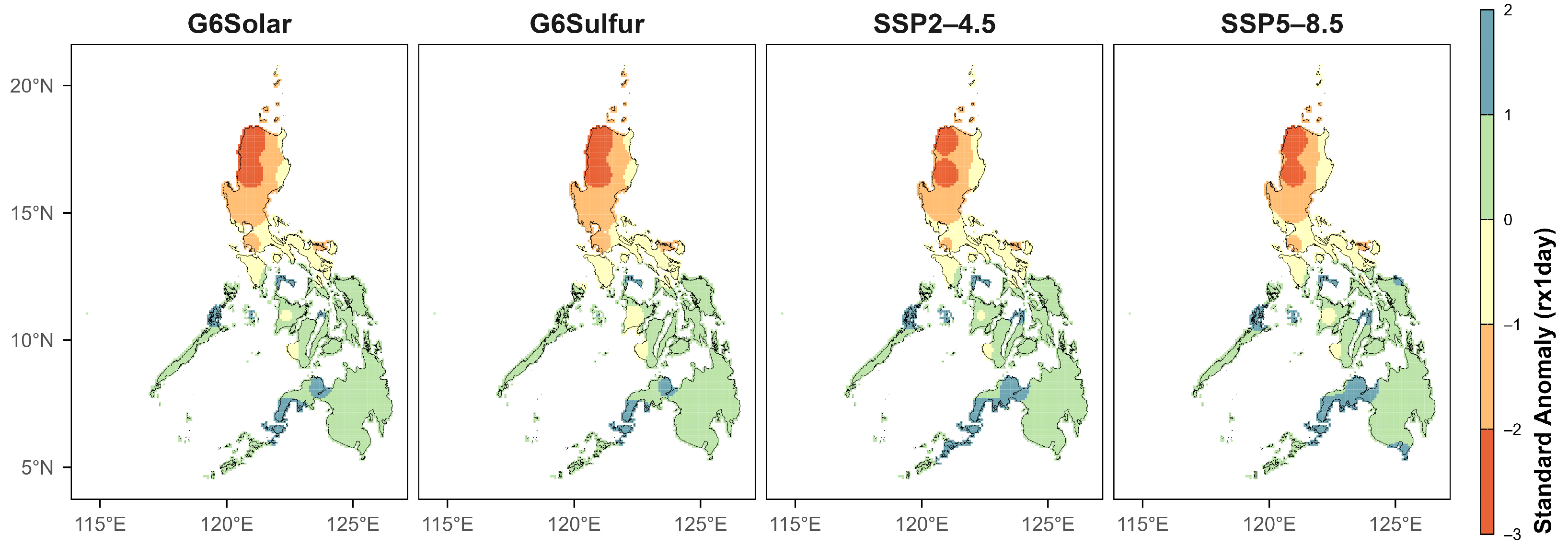
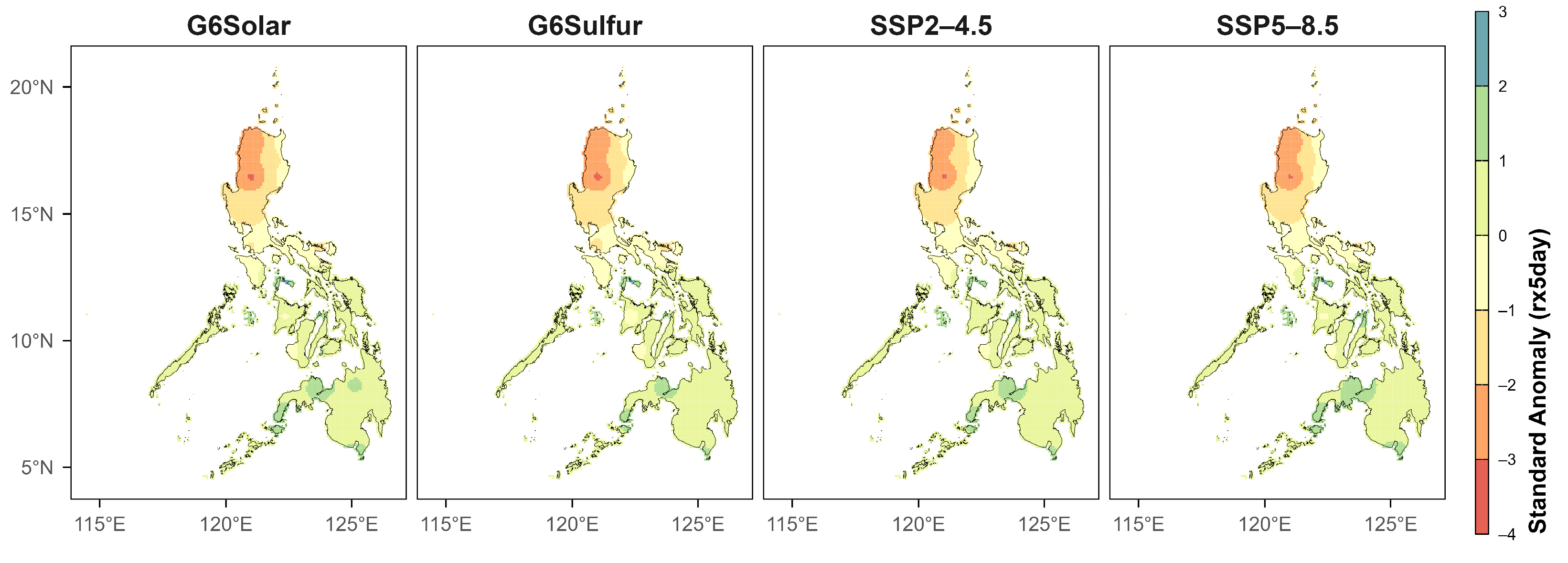
The multi-model ensemble average change in monthly extreme 1-day (RX1day) and 5-day precipitation (RX5day) exhibits a distinct geographical variance under different scenarios, as shown in Figure 3 and Figure 4. There is an evident north–south dipole pattern in RX1day as increasing patterns are expected in the southern portions of the country, while the northern portions are expected to behave otherwise. The spatial extent of this rainfall reduction in the north is larger under the geoengineering scenarios (G6Solar and G6Sulfur) than under the standard climate change scenarios. SSP2-4.5 and SSP5-8.5 project a more expansive increase in extreme rainfall across the southwestern regions, with positive standardized differences reaching a maximum of approximately 2. The changes in RX5day also show differences between the northern and southern portions of the country. All scenarios show a greater decrease in extreme rainfall in the northern region with the anomaly reaching a maximum value of 4. While this phenomenon is observed across all scenarios, a larger area of potentially drier-than-usual conditions is present under both G6Solar and G6Sulfur than under SSP2-4.5 and SSP5-8.5.

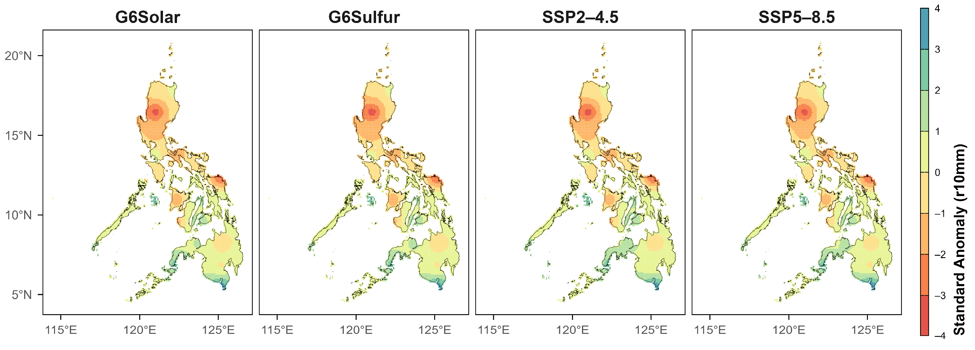
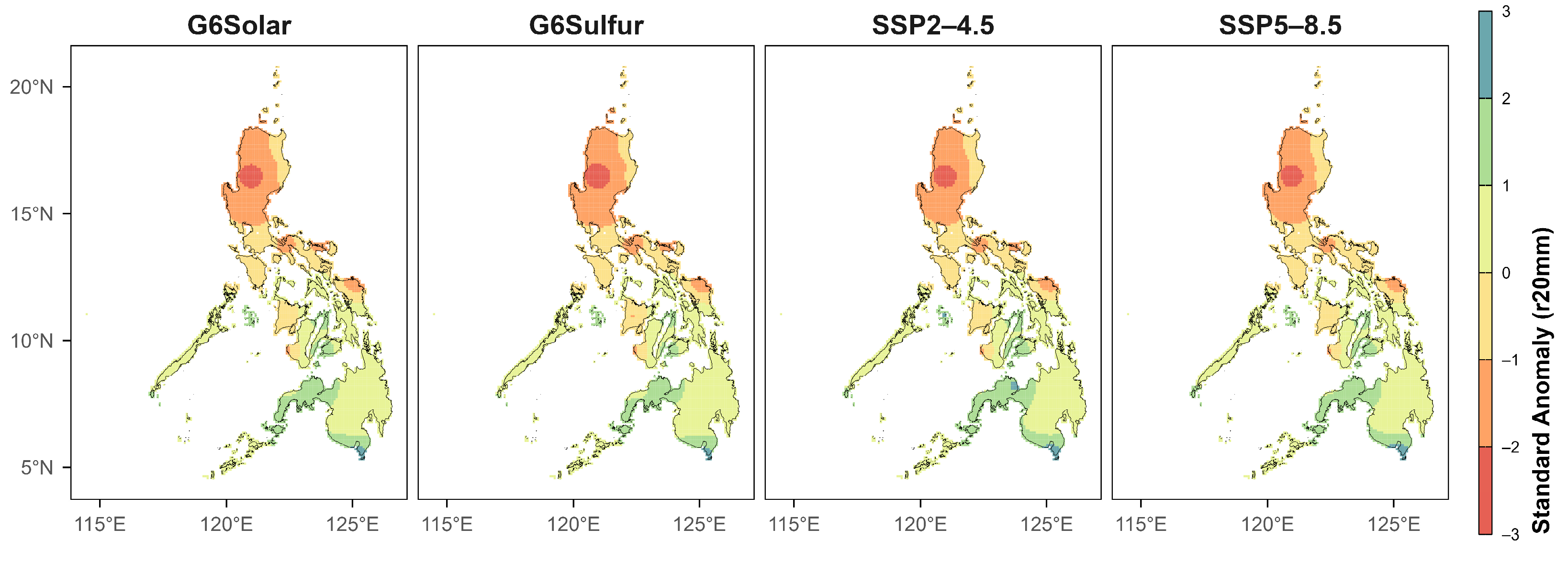
Figure 5 and Figure 6 illustrate the ensemble mean number of days with heavy (R10mm) and very heavy (R20mm) precipitation over the 30 years. Changes in both indices vary spatially across the country but with minimal differences between scenarios. Most regions show a decrease in both R10mm and R20mm suggesting drier conditions across portions of Luzon and the Visayas due to fewer days with at least 10 mm of rainfall. Parts of Mindanao and central portions of the country are projected to see increases in these indices. In terms of anomaly magnitude, future projections of R10mm exhibit larger negative anomalies than R20mm, indicating that the number of days with at least 10 mm of precipitation will decrease more drastically than the number of days with at least 20 mm.

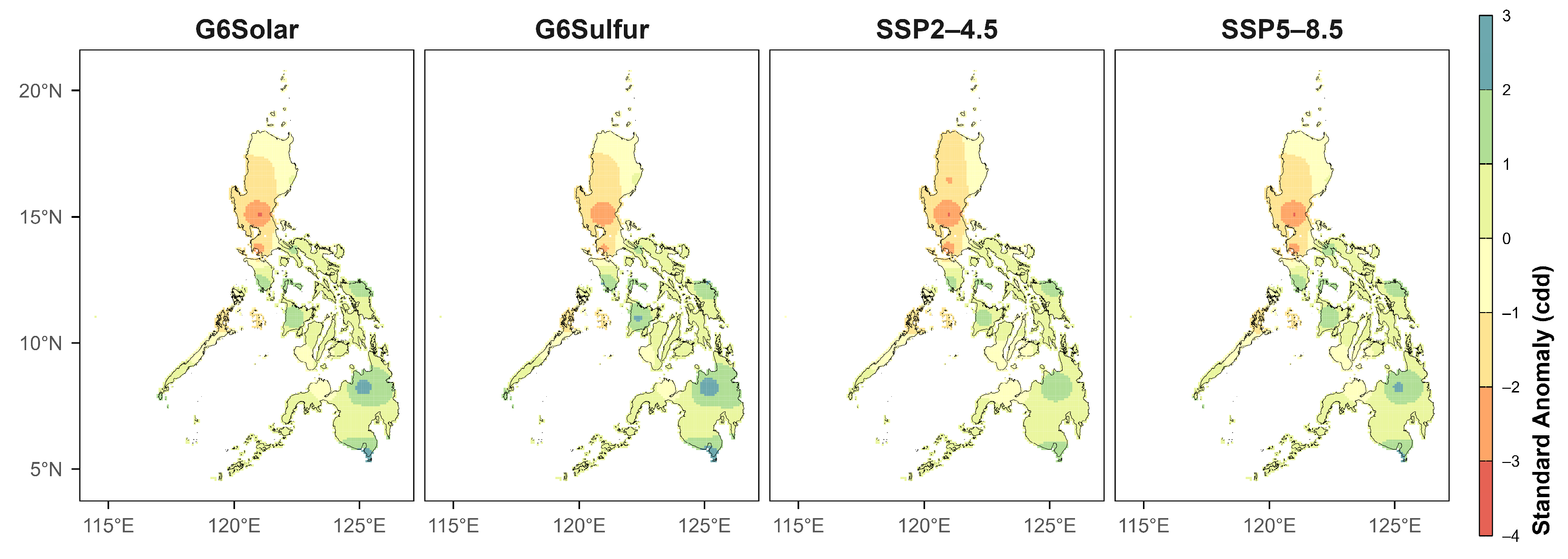
The results on consecutive dry days (CDDs)(Figure 7) show spatial and scenario-dependent variations across the Philippines. Across all scenarios, most regions exhibit increases in the number of consecutive dry days except in northern portions of Luzon. Anomalies of at least +2 in CDDs are observed under G6Solar, G6Sulfur, and SSP5-8.5 in the southern portions of the country. Both G6Solar and G6Sulfur project a wider spatial extent of elevated CDDs than SSP5-8.5, although G6Solar also shows relatively larger areas with lower or even negative anomalies.

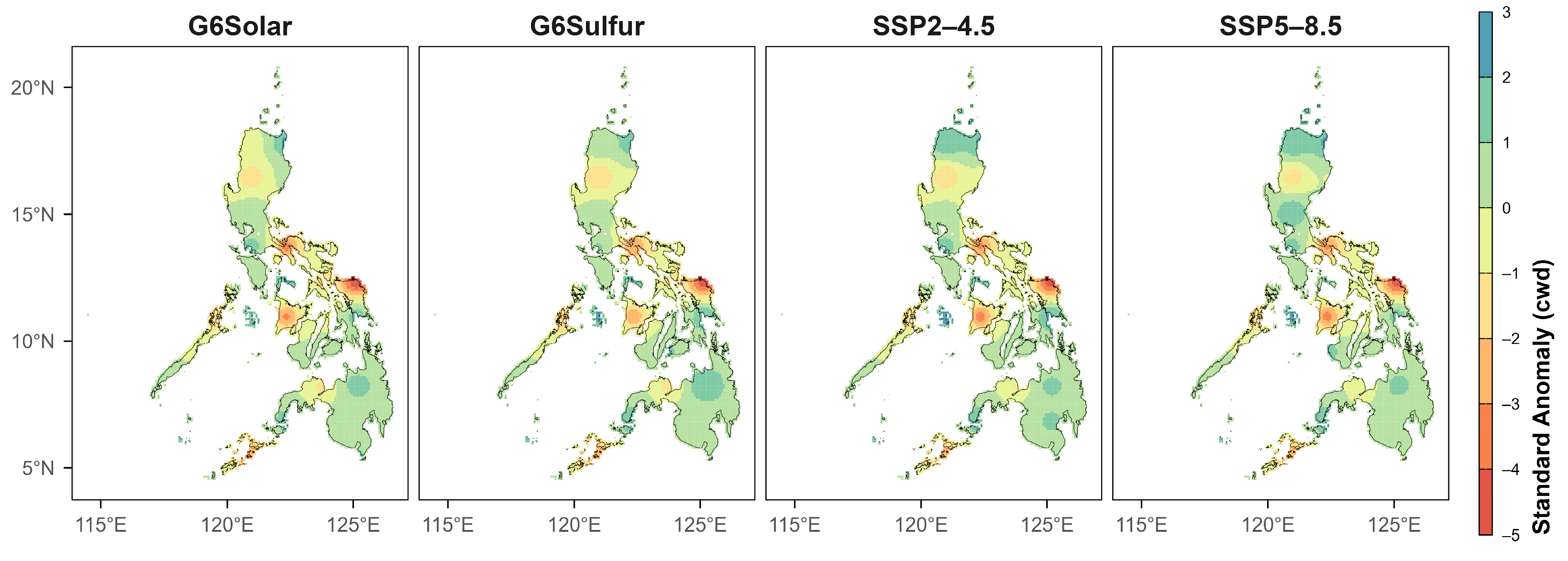
Figure 8 illustrates changes in the consecutive wet days (CWDs) per scenario across the Philippines. The results show that the anomalies in CWDs are spatially distributed and vary by scenario. Across all scenarios, increases in CWDs are likely to occur around Visayas and central portions of Luzon, suggesting longer wet spells. Negative anomalies, with some reaching −5, are evident across all scenarios, with G6Solar showing the widest spatial extent. The areas likely to experience an increase in CWDs are larger under both SSP2-4.5 and SSP5-8.5.

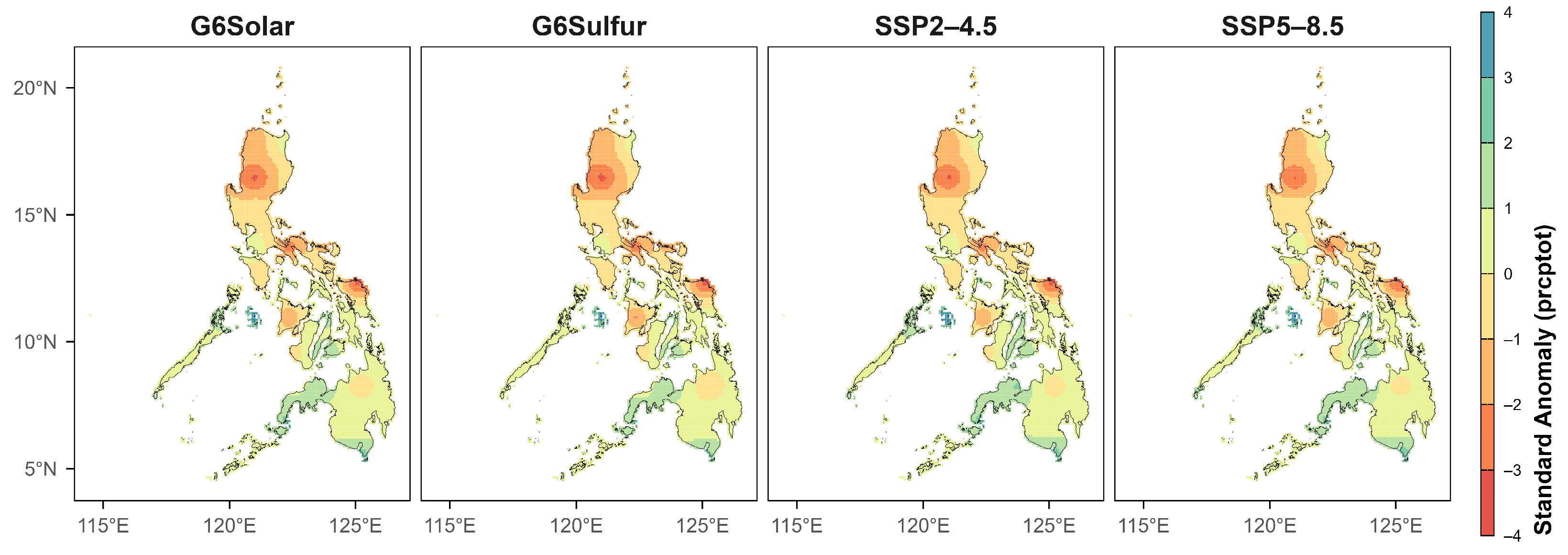
The total annual precipitation (PRCPTOT) in Figure 9 shows differences between the northern and southern portions of the study area in future projections. Generally, areas in the northern portion of the country exhibit decreasing PRCPTOT, with anomalies of at least 0 or below. Southern regions are likely to experience more PRCPTOT than indicated in baseline data. Among the scenarios, G6Sulfur shows a larger area with higher anomaly values, especially in the eastern and central portions of the country. This suggests that drier conditions are expected in regions around the Visayas and Luzon Island.

3.2. Variability in Extreme Temperature Indices

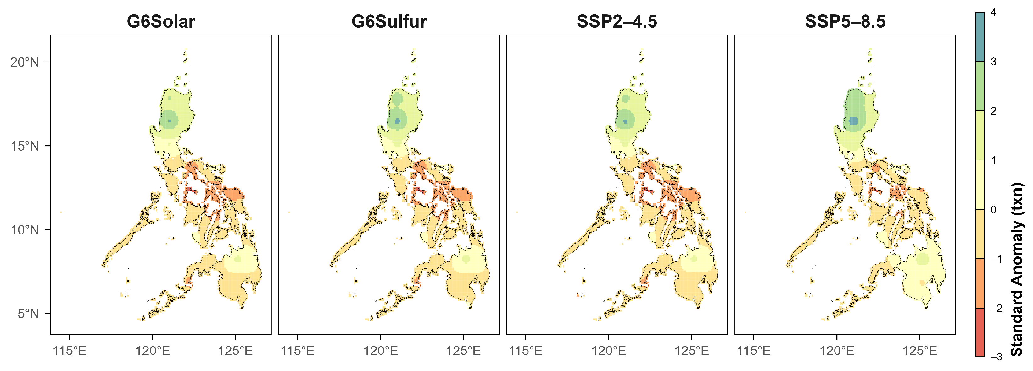
The multi-model ensemble average of the annual minimum daily maximum temperature (TXn) shows a distinct spatial divergence between the northern and southern portions of the Philippines (Figure 10). Future projections across all scenarios suggest that the northern parts of Luzon and Mindanao will likely experience increases in TXn, with the northern regions showing larger positive anomalies. Decreases in TXn are prominently observed in the Visayas and other parts of Mindanao, where negative anomalies dominate. Among the scenarios, G6Solar projects the widest spatial extent of strong decreases in anomalies, with values reaching at least −3 across large portions of the country. While SSP5-8.5 indicates that most regions will undergo a more gradual decline, with anomalies ranging from −2 to +4, it also shows broader areas characterized by increasing trends.

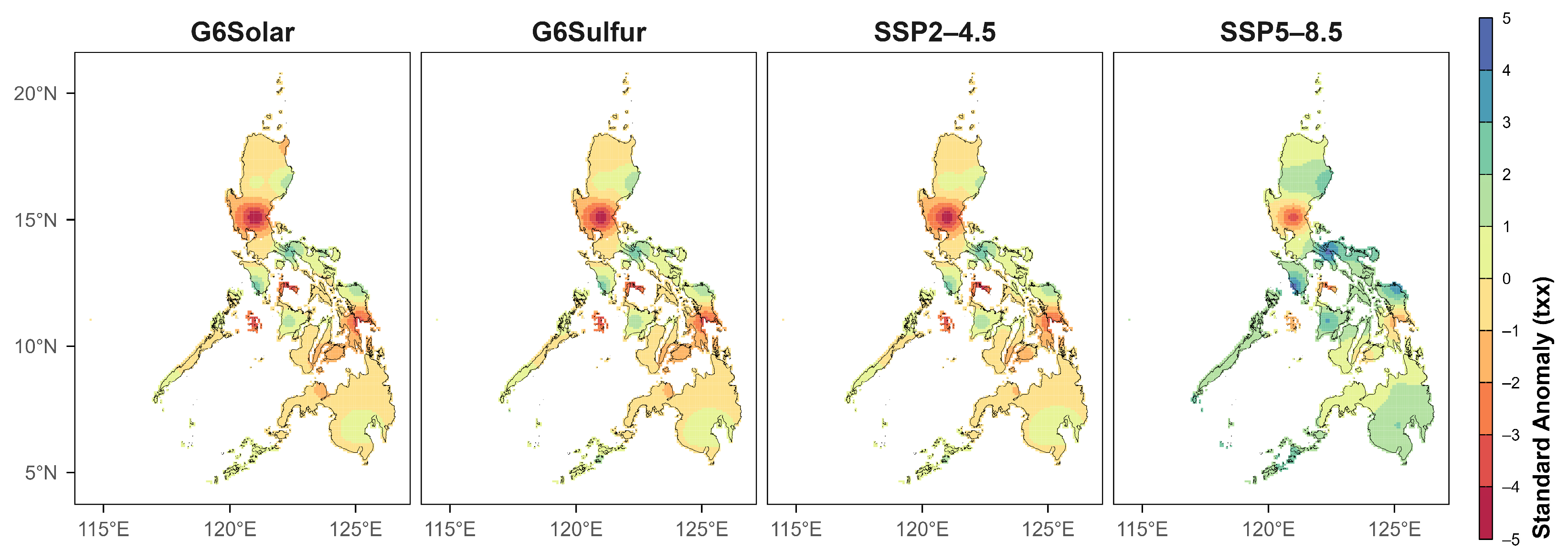
Results for the annual maximum value of daily maximum temperature (TXx), (Figure 11) vary spatially across the Philippines with notable variability in magnitude across scenarios. In all cases, a strong decrease in TXx is evident in the central regions of Luzon. Among the scenarios, G6Solar projects the broadest spatial extent of negative anomalies and the smallest area with increasing TXx, suggesting a more consistent cooling effect. SSP5-8.5 indicates that most regions are likely to experience future increases in TXx, highlighting widespread intensification of extreme heat under high-emission conditions.

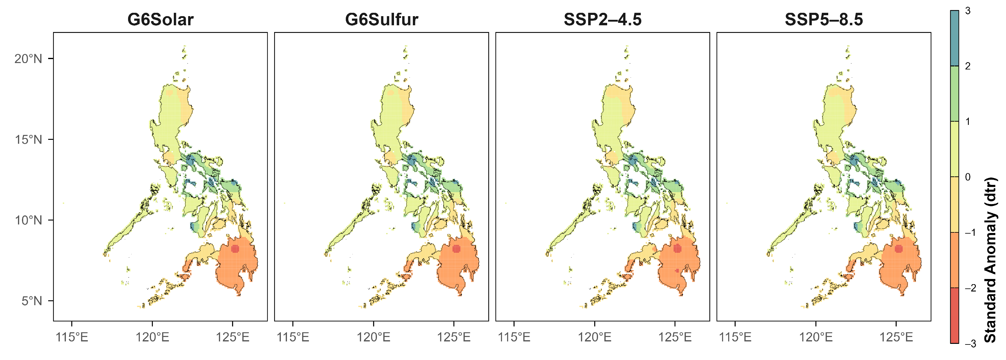
The change in diurnal temperature range (DTR) has only slight variations across different scenarios (Figure 12). Consistent across all scenarios, areas around the Visayas Islands and the southern portions of Luzon Island are observed to have a higher DTR. For G6Solar and G6Sulfur, larger areas with increasing DTR are observed in the northwestern portions of the country. Slightly more areas with decreasing DTR are observed on the island of Mindanao under SSP2-4.5.

3.3. Temporal Analysis of Climate Extremes

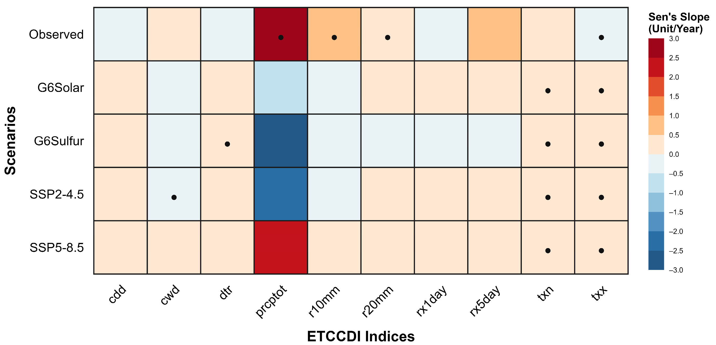
The trends in climate indices and their level of significance under different scenarios were determined using Sen’s slope and the Mann–Kendall test, as shown in Figure 13. For CDDs, the observed record indicates a weak decreasing trend, yet future scenarios project a reversal toward increasing slopes. CWDs show a historically increasing trend that persists under SSP5-8.5, but both G6Solar and G6Sulfur suggest declines, with SSP2-4.5 showing a statistically significant downward trend. For PRCPTOT, R10mm, and R20mm, the slopes generally show a significant upward trend in historical observations and continue to increase under SSP5-8.5, albeit at a lower rate. Future projections of PRCPTOT and R10mm under G6Solar, G6Sulfur, and SSP2-4.5 show a shift toward a decreasing slope, though this is observed only for R20mm under G6Sulfur. Given the historical downward trend in RX1day and the upward trend in RX5day, it was expected to show a decreasing trend under G6Sulfur but an increasing trend under G6Solar, SSP2-4.5, and SSP5-8.5.

The slope of TXn consistently shows a positive trend that becomes statistically significant across all scenarios in future scenarios. TXx shows a significant decreasing trend that shifts toward statistically significant positive slopes in future projections. For DTR, the significantly decreasing slope in the historical observations shifts to a positive slope across all future scenarios but remains significant only under G6Sulfur.

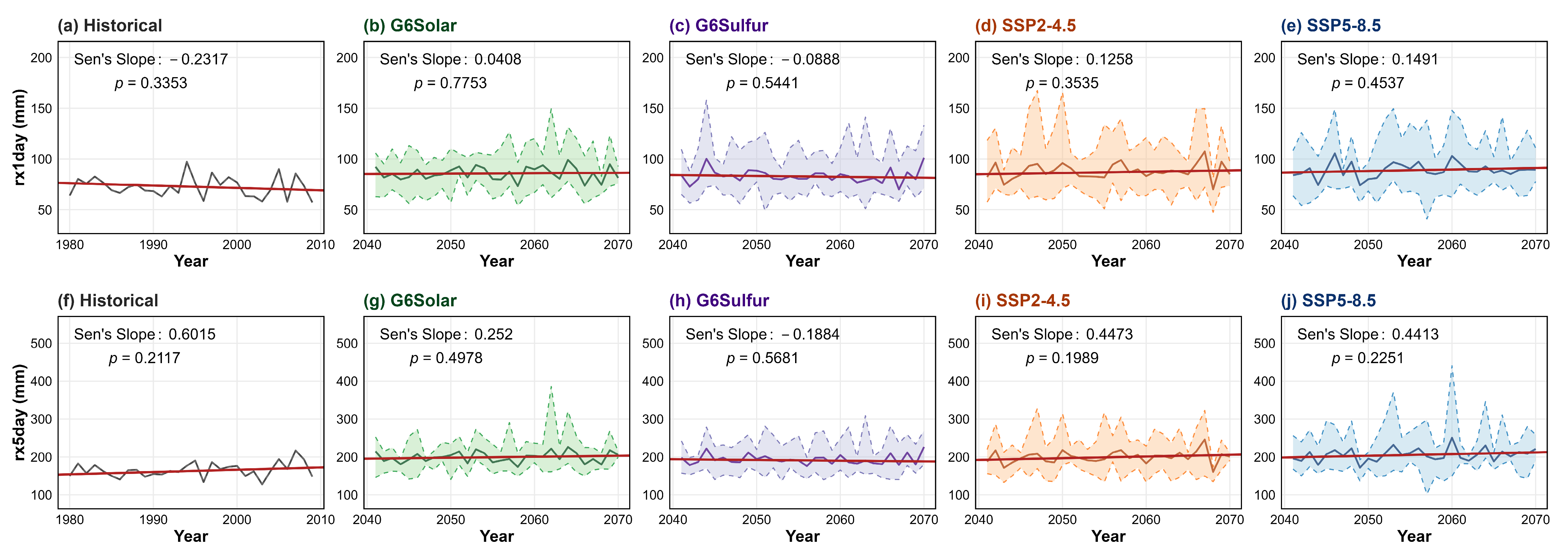
The 30-year future projections for RX1day and RX5day show variability relative to historical observations and differ across scenarios. Figure 14 shows that RX1day has historically declined, but most scenarios show an overall upward trend. SSP5-8.5 shows a stronger average increasing trend of 0.1491 mm per year compared to both G6Solar and SSP2-4.5, which show 0.0408 and 0.1258 mm per year, respectively. Among the scenarios, only G6Sulfur shows a decreasing trend, with an average rate of 0.0888 mm per year. Meanwhile, historical and future trends in RX5day mostly show increases, except for under G6Sulfur.

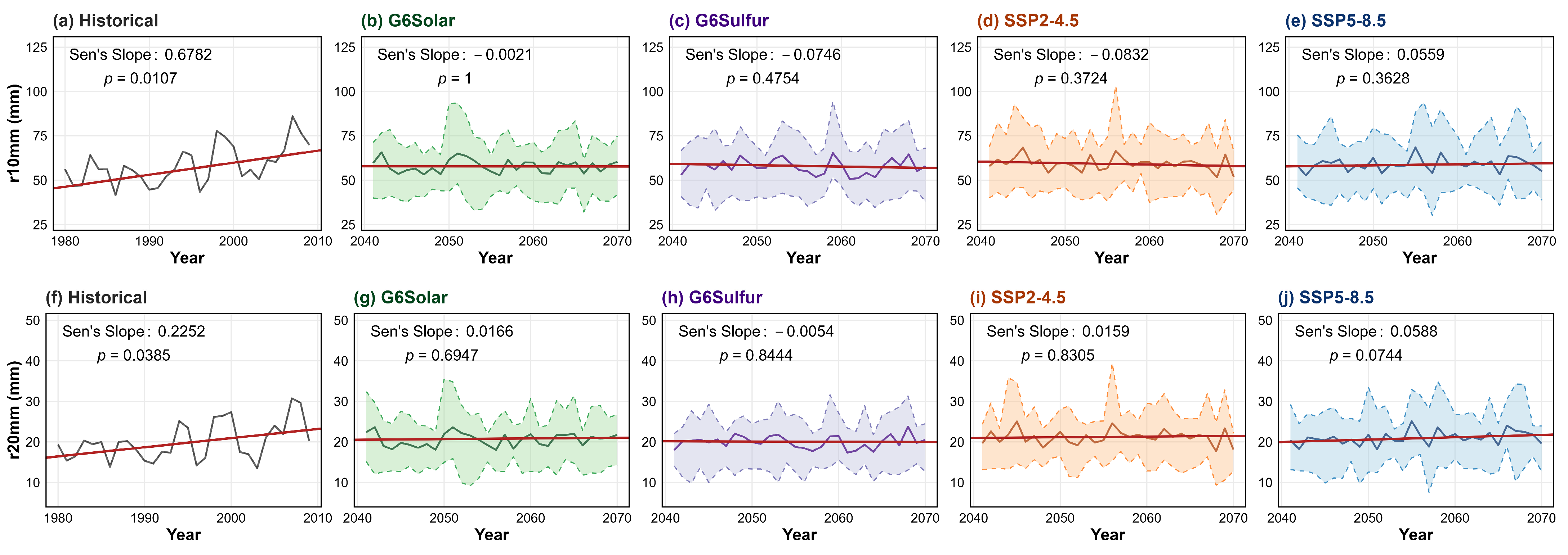
The historical and future trends in R10mm and R20mm (Figure 15) indicate that the steep and statistically significant increases observed in the historical record (0.6782 and 0.2252 days per year, respectively) are projected to attenuate in magnitude under future scenarios. For R10mm, negative slopes ranging from −0.0021 to −0.0832 days per year are evident under G6Solar, G6Sulfur, and SSP2-4.5, while a weak positive slope of 0.0559 days per year is projected under SSP5-8.5. For R20mm, a negative slope (−0.0054 days per year) is only observed under G6Sulfur, whereas positive slopes ranging from 0.0159 to 0.0588 days per year are projected under G6Solar, SSP2-4.5, and SSP5-8.5.

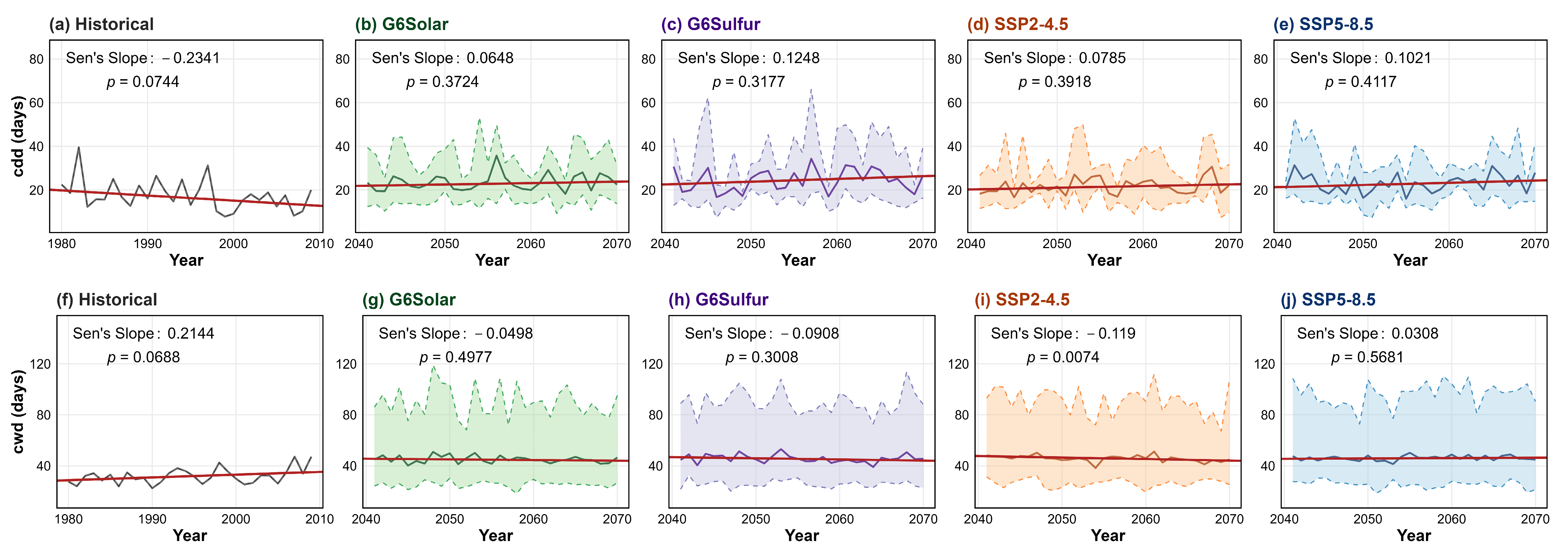
Figure 16 shows the historical and projected slopes of CDDs and CWDs across scenarios, respectively, highlighting the contrasting tendencies between dry and wet spell durations. The historical trend in CDDs shows a decreasing slope, but all future scenarios project positive slopes, indicating longer dry spells. For CWDs, the observed data show a slightly positive slope, but future scenarios indicate negative slopes in most scenarios. Negative slopes are observed under G6Solar, G6Sulfur, and SSP2-4.5, whereas SSP5-8.5 projects a weak positive slope, suggesting that prolonged wet spells may decrease under most pathways, except for in the high-emission scenario.

Figure 17 shows the difference in the historical and future trends in PRCPTOT. Historically, PRCPTOT shows a statistically significant positive slope of 16.66, indicating a strong increasing trend in precipitation. For the future scenarios, G6Solar, G6Sulfur, and SSP2-4.5 all show negative slopes, suggesting slight decreases in precipitation, though none are statistically significant. SSP5-8.5 projects a positive slope, pointing toward an increasing trend in precipitation, but this increase is not statistically significant.

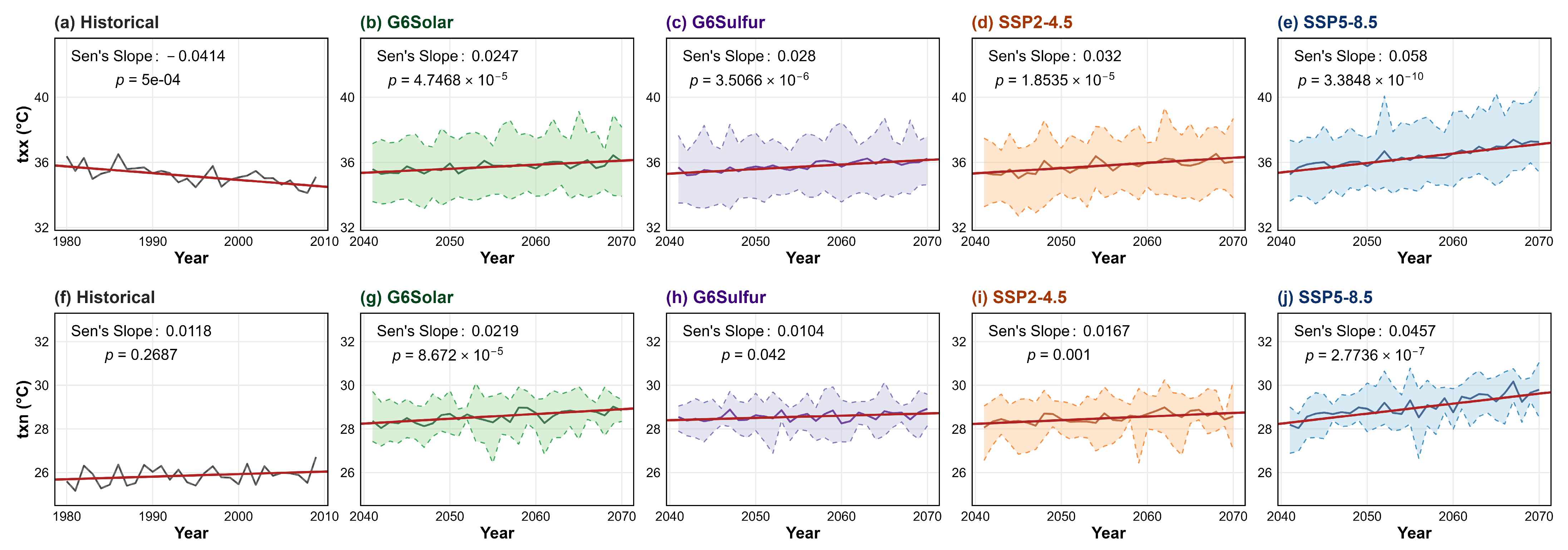
Figure 18 shows the historical and projected slopes of TXx and TXn, highlighting changes in slope behavior and steepness. TXx has historically shown a statistically significant downward trend. All future scenarios project statistically significant positive slopes. In both past and future scenarios, the TXn trend shows a positive slope. The increasing trend in TXn is not statistically significant. Future projections, however, exhibit significantly positive slopes. For both indices, steep and statistically significant increasing slopes are evident under the SSP5-8.5 scenario, whereas more moderate yet still significant increases are observed under the scenarios incorporating SRM interventions.

The historical record exhibits a weak negative slope, while all future scenarios project positive slopes. Among these, G6Solar, SSP2-4.5, and SSP5-8.5 show modest but non-significant warming, while G6Sulfur demonstrates a statistically significant increase. However, in future projections, DTR trends appear to be nearly flat, with values clustering around 7 °C and slopes being close to zero (0.0012 to 0.0022). These extremely low values, as shown in Figure 19, might be due to errors in the selected models, which removed natural year-to-year variability, resulting in artificially uniform projections.

3.4. Ensemble Sensitivity and Trend Robustness Analysis

To further evaluate the unrealistic physical data trends observed in the projections of CESM2-WACCM6, a Leave-One-Out (LOO) sensitivity analysis was performed to isolate its effects on the multi-model consensus.

Table 4. Sensitivity analysis of multi-model mean temperature trends to the exclusion of the CESM2-WACCM6 model.

Parameter	Scenario	With CESM2-WACCM6		Without CESM2-WACCM6		ΔSS
		SS	p-Value	SS	p-Value
TXn	G6Solar	0.0219	8.6720 × 10−5	0.0213	4.0000 × 10−4	0.0006
	G6Sulfur	0.0104	4.2000 × 10−2	0.0100	2.9500 × 10−2	0.0004
	SSP2-4.5	0.0167	1.0000 × 10−3	0.0138	1.5300 × 10−2	0.0029
	SSP5-8.5	0.0457	2.7736 × 10−7	0.0462	4.8749 × 10−4	−0.0005
TXx	G6Solar	0.0247	4.7468 × 10−5	0.0238	8.0000 × 10−4	0.0009
	G6Sulfur	0.0280	3.5066 × 10−6	0.0250	7.4728 × 10−5	0.003
	SSP2-4.5	0.0320	1.8535 × 10−5	0.0332	6.4315 × 10−5	−0.0012
	SSP5-8.5	0.0580	3.3848 × 10−10	0.0569	3.1569 × 10−9	0.0011
DTR	G6Solar	0.0017	0.0688	0.0021	0.0688	−0.0004
	G6Sulfur	0.0022	0.0457	0.0028	0.0457	−0.0006
	SSP2-4.5	0.0012	0.0744	0.0016	0.0804	−0.0004
	SSP5-8.5	0.0022	0.0688	0.0028	0.0688	−0.0006

contrasts the Sen’s slope and Mann–Kendall p-values of the five-model ensemble against those of the revised multi-model ensemble omitting CESM2-WACCM6.

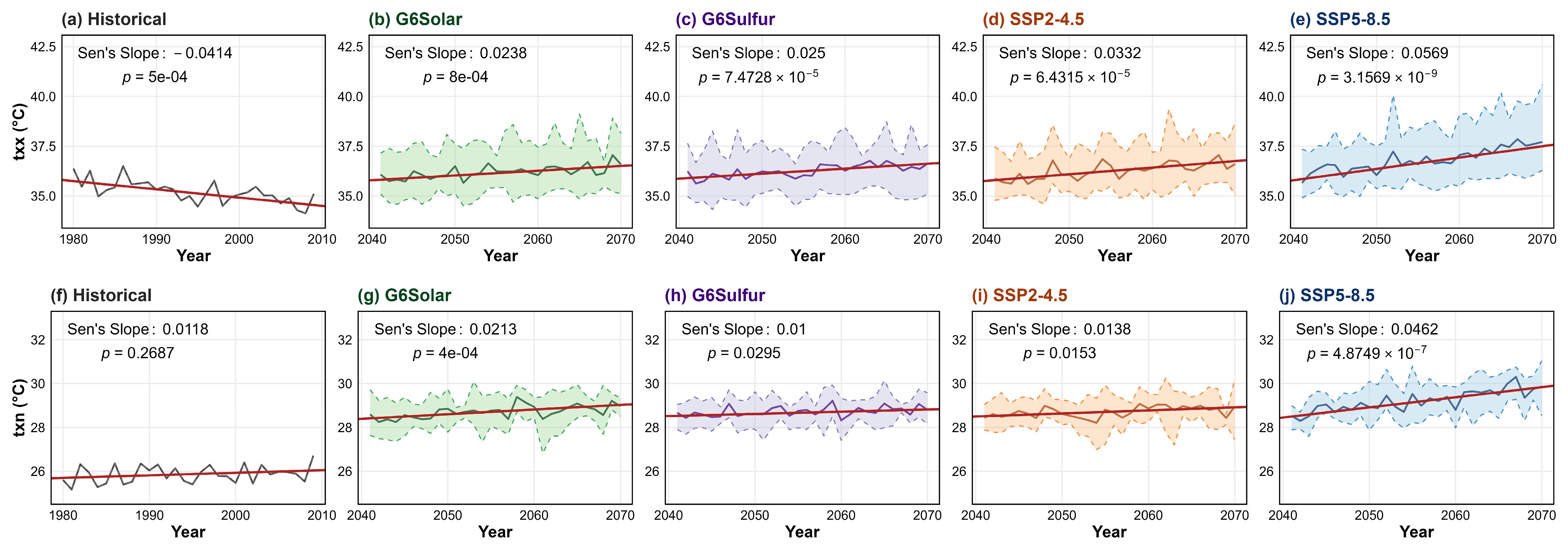
Table 4 summarizes the results of the sensitivity analysis in MME with and without the CESM2-WACCM6 model. The Mann–Kendall and Sen’s slope analysis reveals that both TXn and TXx exhibit statistically significant increasing trends across all scenarios. For TXn, the Sen’s slope values range from approximately 0.010 to 0.046, with p-values well below the 0.05 threshold, indicating robust upward trends in cold-side temperature extremes. The comparison between simulations performed with and without CESM2-WACCM6 shows only marginal differences in the magnitude of the slope (ΔSS between −0.0005 and +0.0029), suggesting that the inclusion of WACCM6 exerts a negligible influence on the long-term trend behavior of TXn. Similarly, TXx displays consistently positive and statistically significant slopes across all scenarios, with Sen’s slope values spanning 0.024–0.058 and p-values typically below 10⁻⁴. These results confirm a strong intensification of warm-side temperature extremes. As with TXn, the ΔSS values for TXx remain very small (−0.0012 to +0.0030), indicating that the presence or absence of CESM2-WACCM6 does not materially alter the detected trends. In contrast, DTR does not exhibit statistically significant trends in any scenario. Although the Sen’s slope values are slightly positive (0.0012–0.0028), the associated p-values (0.0457–0.0804) exceed the significance threshold, implying that the observed changes are not statistically robust. The ΔSS values are uniformly small and negative (−0.0004 to −0.0006), further supporting the conclusion that the diurnal temperature range remains statistically stable regardless of the inclusion of WACCM6. Overall, the results demonstrate that temperature extremes (TXn and TXx) intensify significantly under all examined scenarios (see Figure 20), whereas DTR shows no statistically significant long-term trend (see Figure 21). The minimal ΔSS values across all variables indicate that the incorporation of CESM2-WACCM6 has only a minor effect on the estimated trend magnitudes.

4. Discussion

The variability in future projections of precipitation indices in terms of rainfall intensity (RX1day and RX5day) and frequency (R10mm and R20mm) from historical observations is less distinct between SRM and non-SRM scenarios. In both scenarios, changes are geographically evident asnorthern portions of the country are projected to have decrease in rainfall intensity and frequency. On the other hand, the southern regions are likely to experience an increase. These geographical variability is also projected in terms of total annual rainfall volume (PRCPTOT) with the north becoming drier and the south receiving more rain than usual. Under SRM scenarios, extreme weather anomalies occur across the central and eastern parts of the country. There are also localized shifts in extreme wet and dry durations across the Philippines. All scenarios project longer dry spells in the south and shorter wet spells in the Visayas and central Luzon but the exact locations of these changes differ significantly.

Although SRM suppresses temperature extremes in the global scale, it deviates from the historical precipitation patterns over the Philippines. Similar to the trends of standard climate change scenarios, it creates a clear north–south hydroclimatic contrast that reduces dryness in northern Luzon and increases rainfall in southern Mindanao with more alignment to future trend projections of moderate-emission scenario than high-emission scenario.. Since SRM selectively reduces surface shortwave radiation while longwave GHG forcing persists, it weakens evaporation and suppresses the global hydrological cycle [12,16,23]. Regionally, SRM reduces the land–sea thermal contrast [58], stabilizes the troposphere [59], and disrupts both ITCZ migration and monsoon dynamics [60,61]. Rather than restoring the hydrological baseline, SRM acts as a novel driver, redistributing regional water availability and exacerbating drought risk in the north and flood risk in the south.

Under extreme temperature indices, SRM pathways successfully mitigate extreme heat, although regional temperature ranges vary. The annual minimum of daily maximum temperature (TXn) shows warming concentrated in northern Luzon and Mindanao and cooling trends prevailing in the Visayas and southern regions. While the annual maximum of daily maximum temperature (TXx) consistently shows strong decreases in central Luzon, differences in scenarios are evident. The SRM scenario induces widespread cooling, while climate change scenarios point to intensified heat extremes. The changes in the diurnal temperature range (DTR) show localized increases in the Visayas and southern Luzon, as well as scenario-specific variations in the northwestern and southern regions.

SRM pathways exert strong thermodynamic control over temperature extremes in the Philippines. Widespread cooling in maximum temperatures reflects direct shortwave scattering by stratospheric aerosols. The spatial variations in minimum temperatures and localized increases in the DTR reflect ongoing longwave GHG forcing, which suppresses night-time radiative cooling. This aligns with the GeoMIP and GLENS studies in Southeast Asia [11,12,17], which show that SRM successfully caps extreme heat but alters tropical precipitation patterns via monsoon and land–sea dynamics. SRM is not a uniform thermostat but an intervention trading thermal stress for hydrological redistribution in island archipelagos.

Temporal analysis of trends in dry and wet spell indicators (CDDs and CWDs) shows contrasting behaviors across scenarios. At the same time, precipitation-related indices (PRCPTOT, R10mm, and R20mm) exhibit significant historical increases that weaken under the SRM scenario. Extreme precipitation indices (RX1day and RX5day) also diverge, reflecting scenario-specific responses. Temperature-related indices consistently show positive slopes, with TXn and TXx transitioning to statistically significant increases and the DTR shifting from a historical decline to positive trends in future projections. Studies focusing on the Southeast Asian region support the notion that, while geoengineering weakens the severe spikes in total and extreme rainfall seen in historical trends, it simultaneously alters dry and wet spell durations and causes extreme temperatures to continue rising under future projections [12,17].

However, future projections show physically unrealistic and invariant trends in CESM2-WACCM6’s DTR index., The error causes future projection panels to lose natural year-to-year fluctuations. The resulting near-zero slopes (0.0012–0.0022) are not indicative of climate responses to solar geoengineering or greenhouse gas forcing; rather, they reflect data errors, rendering these projections unsuitable for physical interpretation. Several studies also suggest that, while CESM2 reliably projects near-term climate trends up to 2050, its long-term projections up to 2100 significantly overestimate global warming due to a structural flaw in its cloud microphysics; this makes the model overly sensitive to carbon dioxide [62,63]. This high climate sensitivity of CESM2-WACCM6 leads to unrealistically extreme future temperatures that contradict both historical observations and prehistoric climate records [64,65], underscoring the need for explicit consideration of this limitation in future multi-model, localized assessments of temperature extremes.

5. Conclusions

The study explores the impacts of solar radiation management in alleviating the effects of climate change on extreme weather events in the Philippines. Future trends indicate that SRM mitigates extreme heat and induces widespread cooling relative to intensifying heat extremes in standard climate change scenarios, it does not restore historical weather patterns. Instead, SRM alters regional climates and worsens the uneven distribution of rainfall. Both SRM and non-SRM scenarios show a localized geographical variation across the country with trends much closer to the moderate emission scenario than the high emission scenario. Northern regions are generally projected to become drier, with decreases in rainfall intensity, frequency, total annual volume, and wet spell duration. Southern regions will generally receive more rain with increased intensity and frequency. SRM introduces its own extreme weather anomalies across the central and eastern parts of the country, alongside localized shifts in wet and dry durations, such as longer dry spells in the south.

The impacts of SRM on daily maximum temperature include reducing the observed trend in historical data. While SRM causes pronounced decreases in the annual maximum in central Luzon and brings cooling trends to the Visayas and Mindanao, warming trends in the annual minimum remain concentrated in northern Luzon and Mindanao. Temperature-related projections from CESM2-WACCM6 should be interpreted with caution given the model’s documented high climate sensitivity. Therefore, this specific model cannot be reliably used to analyze future temperature responses to greenhouse gas forcing or solar geoengineering.

These countrywide impacts of SRM on future precipitation and temperature will affect how adjustments can be made to temper the impacts of global warming, even as rainfall amounts and intensity increase in some areas. With the impacts varying geographically and at localized scales, adjustments need to be made at the local level. Corresponding policies need to be put in place to safeguard various stakeholders who might be affected by the potential implementation of SRM.

References

1. Naz, R.; Shah, M.; Ullah, A.; Alam, I.; Khan, Y. An Assessment of Effects of Climate Change on Human Lives in Context of Local Response to Agricultural Production in District Buner. Sarhad J. Agric. 2020, 36, 110–119. [Google Scholar] [CrossRef] [Scilit]
2. IPCC. 2023 Summary for Policymakers. In Climate Change 2023: Synthesis Report. Contribution of Working Groups I, II and III to the Sixth Assessment Report of the Intergovernmental Panel on Climate Change; Core Writing Team, Lee, H., Romero, J., Eds.; IPCC: Geneva, Switzerland, 2023. [Google Scholar]
3. Nguyen-Sy, T.; Cheng, W.; Tawaraya, K.; Sugawara, K.; Kobayashi, K. Impacts of Climatic and Varietal Changes on Phenology and Yield Components in Rice Production in Shonai Region of Yamagata Prefecture, Northeast Japan for 36 Years. Plant Prod. Sci. 2019, 22, 382–394. [Google Scholar] [CrossRef] [Scilit]
4. Magazzino, C.; Mutascu, M.; Sarkodie, S.A.; Adedoyin, F.F.; Owusu, P.A. Heterogeneous Effects of Temperature and Emissions on Economic Productivity across Climate Regimes. Sci. Total Environ. 2021, 775, 145893. [Google Scholar] [CrossRef] [Scilit]
5. Sovacool, B.K.; Baum, C.M.; Low, S. Determining Our Climate Policy Future: Expert Opinions about Negative Emissions and Solar Radiation Management Pathways. Mitig. Adapt. Strateg. Glob. Chang. 2022, 27, 58. [Google Scholar] [CrossRef] [Scilit] [PubMed]
6. Tan, M.L.; Juneng, L.; Kuswanto, H.; Do, H.X.; Zhang, F. Impacts of Solar Radiation Management on Hydro-Climatic Extremes in Southeast Asia. Water 2023, 15, 1089. [Google Scholar] [CrossRef] [Scilit]
7. Effiong, U.; Neitzel, R.L. Assessing the Direct Occupational and Public Health Impacts of Solar Radiation Management with Stratospheric Aerosols. Environ. Health 2016, 15, 7. [Google Scholar] [CrossRef] [Scilit] [PubMed]
8. MacMartin, D.G.; Ricke, K.L.; Keith, D.W. Solar Geoengineering as Part of an Overall Strategy for Meeting the 1.5°C Paris Target. Philos. Trans. A Math. Phys. Eng. Sci. 2018, 376, 20160454. [Google Scholar] [CrossRef] [Scilit] [PubMed]
9. Sugiyama, M.; Asayama, S.; Kosugi, T.; Ishii, A.; Watanabe, S. Public Attitude toward Solar Radiation Modification: Results of a Two-Scenario Online Survey on Perception in Four Asia–Pacific Countries. Sustain. Sci. 2025, 20, 423–438. [Google Scholar] [CrossRef] [Scilit]
10. Kravitz, B.; Robock, A.; Tilmes, S.; Boucher, O.; English, J.M.; Irvine, P.J.; Jones, A.; Lawrence, M.G.; MacCracken, M.; Muri, H.; et al. The Geoengineering Model Intercomparison Project Phase 6 (GeoMIP6): Simulation Design and Preliminary Results. Geosci. Model Dev. 2015, 8, 3379–3392. [Google Scholar] [CrossRef] [Scilit]
11. Jones, A.; Haywood, J.M.; Jones, A.C.; Tilmes, S.; Kravitz, B.; Robock, A. North Atlantic Oscillation Response in GeoMIP Experiments G6solar and G6sulfur: Why Detailed Modelling Is Needed for Understanding Regional Implications of Solar Radiation Management. Atmos. Chem. Phys. 2021, 21, 1287–1304. [Google Scholar] [CrossRef] [Scilit]
12. Narenpitak, P.; Kongkulsiri, S.; Tomkratoke, S.; Sirisup, S. Regional Impacts of Solar Radiation Modification on Surface Temperature and Precipitation in Mainland Southeast Asia and the Adjacent Oceans. Sci. Rep. 2024, 14, 22713. [Google Scholar] [CrossRef] [Scilit] [PubMed]
13. Tye, M.R.; Dagon, K.; Molina, M.J.; Richter, J.H.; Visioni, D.; Kravitz, B.; Tebaldi, C.; Tilmes, S. Indices of Extremes: Geographic Patterns of Change in Extremes and Associated Vegetation Impacts under Climate Intervention. EGUsphere 2022, 13, 1233–1257. [Google Scholar] [CrossRef] [Scilit]
14. Irvine, P.J.; Keith, D.W. Halving Warming with Stratospheric Aerosol Geoengineering Moderates Policy-Relevant Climate Hazards. Environ. Res. Lett. 2020, 15, 44011. [Google Scholar] [CrossRef] [Scilit]
15. de Perez, E.; Fuentes, I.; Jack, C.; Kruczkiewicz, A.; Pinto, I.; Stephens, E. Different Types of Drought under Climate Change or Geoengineering: Systematic Review of Societal Implications. Front. Clim. 2022, 4, 959519. [Google Scholar] [CrossRef] [Scilit]
16. Ricke, K.; Wan, J.S.; Saenger, M.; Lutsko, N.J. Hydrological Consequences of Solar Geoengineering. Annu. Rev. Earth Planet. Sci. 2023, 51, 447–470. [Google Scholar] [CrossRef] [Scilit]
17. Tang, A.; Kemp, L. A Fate Worse than Warming? Stratospheric Aerosol Injection and Global Catastrophic Risk. Front. Clim. 2021, 3, 720312. [Google Scholar] [CrossRef] [Scilit]
18. Tracy, S.M.; Moch, J.M.; Eastham, S.D.; Buonocore, J.J. Stratospheric Aerosol Injection May Impact Global Systems and Human Health Outcomes. Elem. Sci. Anth. 2022, 10, 47. [Google Scholar] [CrossRef] [Scilit]
19. Wheeler, L.; Zeitler, T.; Brunell, S.; Lien, J.; Shand, L.; Wagman, B.; Martinez, C.; Potter, K. Performance Assessment for Climate Intervention (PACI): Preliminary Application to a Stratospheric Aerosol Injection Scenario. Front. Environ. Sci. 2023, 11, 1205515. [Google Scholar] [CrossRef] [Scilit]
20. Tilmes, S.; Rosenlof, K.H.; Visioni, D.; Bednarz, E.M.; Felgenhauer, T.; Smith, W.; Lennard, C.; Diamond, M.S.; Henry, M.; Harrison, C.S.; et al. Research Criteria towards an Interdisciplinary Stratospheric Aerosol Intervention Assessment. Oxf. Open Clim. Change 2024, 4, kgae010. [Google Scholar] [CrossRef] [Scilit]
21. Visioni, D.; Robock, A.; Haywood, J.; Henry, M.; Tilmes, S.; MacMartin, D.G.; Kravitz, B.; Doherty, S.J.; Moore, J.; Lennard, C.; et al. G6-1.5 K-SAI: A New Geoengineering Model Intercomparison Project (GeoMIP) Experiment Integrating Recent Advances in Solar Radiation Modification Studies. Geosci. Model Dev. 2024, 17, 2583–2596. [Google Scholar] [CrossRef] [Scilit]
22. Lockley, A.; Xu, Y.; Tilmes, S.; Sugiyama, M.; Rothman, D.; Hindes, A. 18 Politically Relevant Solar Geoengineering Scenarios. Socio-Environ. Syst. Model. 2022, 4, 18127. [Google Scholar] [CrossRef] [Scilit]
23. Honegger, M.; Michaelowa, A.; Pan, J. Potential Implications of Solar Radiation Modification for Achievement of the Sustainable Development Goals. Mitig. Adapt. Strateg. Glob. Chang. 2021, 26, 21. [Google Scholar] [CrossRef] [Scilit]
24. Enevoldsen, P.; Baum, C.M.; Low, S.; Sovacool, B.K. Examining the Synergies and Tradeoffs of Net-Zero Climate Protection with the Sustainable Development Goals. Sci. Prog. 2022, 105, 00368504221138443. [Google Scholar] [CrossRef] [Scilit] [PubMed]
25. Dipu, S.; Quaas, J.; Quaas, M.; Rickels, W.; Mülmenstädt, J.; Boucher, O. Substantial Climate Response Outside the Target Area in an Idealized Experiment of Regional Radiation Management. Climate 2021, 9, 66. [Google Scholar] [CrossRef] [Scilit]
26. Nyunt, C.T.; Koike, T.; Yamamoto, A. Statistical Bias Correction for Climate Change Impact on the Basin Scale Precipitation in Sri Lanka, Philippines, Japan and Tunisia. Hydrol. Earth Syst. Sci. Discuss. 2016, 2016, 1–32. [Google Scholar] [CrossRef] [Scilit]
27. Shope, C.L.; Maharjan, G.R. Modeling Spatiotemporal Precipitation: Effects of Density, Interpolation, and Land Use Distribution. Adv. Meteorol. 2015, 2015, 174196. [Google Scholar] [CrossRef] [Scilit]
28. Han, Z.; He, Y.; Liu, G.; Perrie, W. Application of Dincae to Reconstruct the Gaps in Chlorophyll-a Satellite Observations in the South China Sea and West Philippine Sea. Remote Sens. 2020, 12, 480. [Google Scholar] [CrossRef] [Scilit]
29. Hisham, M.B.; Yaakob, S.N.; Raof, R.A.; Nazren, A.B.; Wafi, N.M. An Analysis of Performance for Commonly Used Interpolation Method. Adv. Sci. Lett. 2017, 23, 5147–5150. [Google Scholar] [CrossRef] [Scilit]
30. National Mapping and Resource Information Authority (NAMRIA). Official Update on the Philippine Island Count: From 7107 to 7641 Islands; National Mapping and Resource Information Authority (NAMRIA): Taguig City, Philippines, 2019. [Google Scholar]
31. Philippine Statistics Authority. Technical Notes on Water Accounts of the Philippines: Flow Accounts; Philippine Statistics Authority: Quezon City, Philippines, 2024. [Google Scholar]
32. Climate Change Commission. Philippines’ First Biennial Transparency Report (BTR) to the United Nations Framework Convention on Climate Change (UNFCCC) Under the Paris Agreement; Climate Change Commission: Manila, Philippines, 2025. [Google Scholar]
33. Rigal, A.; Azaïs, J.-M.; Ribes, A. Estimating Daily Climatological Normals in a Changing Climate. Clim. Dyn. 2019, 53, 275–286. [Google Scholar] [CrossRef] [Scilit]
34. Hulme, M. Climates Multiple: Three Baselines, Two Tolerances, One Normal. Acad. Lett. 2021. [Google Scholar] [CrossRef] [Scilit]
35. Ikoma, E.; Kitsuregawa, M. DIAS—Earth Environment Data Integration and Analysis System. Commun. ACM 2023, 66, 85–86. [Google Scholar] [CrossRef] [Scilit]
36. Yatagai, A.; Maeda, M.; Khadgarai, S.; Masuda, M.; Xie, P. End of the Day (EOD) Judgment for Daily Rain-Gauge Data. Atmosphere 2020, 11, 772. [Google Scholar] [CrossRef] [Scilit]
37. Sunilkumar, K.; Yatagai, A.; Masuda, M. Preliminary Evaluation of GPM-IMERG Rainfall Estimates over Three Distinct Climate Zones with APHRODITE. Earth Space Sci. 2019, 6, 1321–1335. [Google Scholar] [CrossRef] [Scilit]
38. Lai, S.; Xie, Z.; Bueh, C.; Gong, Y. Fidelity of the APHRODITE Dataset in Representing Extreme Precipitation over Central Asia. Adv. Atmos. Sci. 2020, 37, 1405–1416. [Google Scholar] [CrossRef] [Scilit]
39. Islam, M.A.; Ahmed, A.; Munir, M.M.; Khandakar, Z.Z. Verification of APHRODITE Precipitation Data Set in Bangladesh. J. Eng. Sci. 2021, 12, 51–56. [Google Scholar] [CrossRef] [Scilit]
40. Jaspe-Santander, C.J.S.; Tabañag, I.D.F. Statistical Performance of Gridded Rainfall Datasets Over Ungauged Jalaur River Basin, Philippines. Nat. Environ. Pollut. Technol. 2024, 23, 1035–1045. [Google Scholar] [CrossRef] [Scilit]
41. Dado, J.M.B.; Takahashi, H.G. Potential Impact of Sea Surface Temperature on Rainfall over the Western Philippines. Prog. Earth Planet. Sci. 2017, 4, 23. [Google Scholar] [CrossRef] [Scilit]
42. Peralta, J.C.A.C.; Narisma, G.T.T.; Cruz, F.A.T. Validation of High-Resolution Gridded Rainfall Datasets for Climate Applications in the Philippines. J. Hydrometeorol. 2020, 21, 1571–1587. [Google Scholar] [CrossRef] [Scilit]
43. Pulatov, A.; Khamidov, A.; Akhmatov, D.; Pulatov, B.; Vasenev, V. Soil Salinity Mapping by Different Interpolation Methods in Mirzaabad District, Syrdarya Province. IOP Conf. Ser. Mater. Sci. Eng. 2020, 883, 12089. [Google Scholar] [CrossRef] [Scilit]
44. Kayıkçı, E.T.; Kazancı, S.Z. Comparison of Regression-Based and Combined Versions of Inverse Distance Weighted Methods for Spatial Interpolation of Daily Mean Temperature Data. Arab. J. Geosci. 2016, 9, 690. [Google Scholar] [CrossRef] [Scilit]
45. Danabasoglu, G.; Lamarque, J.-F.; Bacmeister, J.; Bailey, D.; Duvivier, A.; Edwards, J.; Emmons, L.; Fasullo, J.; Garcia, R.; Gettelman, A.; et al. The Community Earth System Model Version 2 (CESM2). J. Adv. Model. Earth Syst. 2020, 12, e2019MS001916. [Google Scholar] [CrossRef] [Scilit]
46. Gettelman, A.; Mills, M.J.; Kinnison, D.E.; Garcia, R.R.; Smith, A.K.; Marsh, D.R.; Tilmes, S.; Vitt, F.; Bardeen, C.G.; McInerny, J.; et al. The Whole Atmosphere Community Climate Model Version 6 (WACCM6). J. Geophys. Res. Atmos. 2019, 124, 12380–12403. [Google Scholar] [CrossRef] [Scilit]
47. Lee, W.R.; Visioni, D.; Wagman, B.M.; Wentland, C.R.; Kravitz, B.; Watanabe, S.; Sekiya, T.; Jones, A.; Haywood, J.; Henry, M.; et al. G6-1.5 K-SAI and G6sulfur: Changes in Impacts and Uncertainty Depending on Stratospheric Aerosol Injection Strategy in the Geoengineering Model Intercomparison Project. EGUsphere 2025, 2025, 1–33. [Google Scholar] [CrossRef] [Scilit]
48. Asner, G.P.; Vaughn, N.R.; Martin, R.E.; Foo, S.A.; Heckler, J.; Neilson, B.J.; Gove, J.M. Mapped Coral Mortality and Refugia in an Archipelago-Scale Marine Heat Wave. Proc. Natl. Acad. Sci. USA 2022, 119, e2123331119. [Google Scholar] [CrossRef] [Scilit] [PubMed]
49. Oshima, N.; Kato, H.; Kadokura, S. An Application of Statistical Downscaling to Estimate Surface Air Temperature in Japan. J. Geophys. Res. Atmos. 2002, 107, ACL 14-1–ACL 14-10. [Google Scholar] [CrossRef] [Scilit]
50. Su, B.; Huang, J.; Gemmer, M.; Jian, D.; Tao, H.; Jiang, T.; Zhao, C. Statistical Downscaling of CMIP5 Multi-Model Ensemble for Projected Changes of Climate in the Indus River Basin. Atmos. Res. 2016, 178, 138–149. [Google Scholar] [CrossRef] [Scilit]
51. Manzanas, R.; Gutiérrez, J.M.; Bhend, J.; Hemri, S.; Doblas-Reyes, F.J.; Penabad, E.; Brookshaw, A. Statistical Adjustment, Calibration and Downscaling of Seasonal Forecasts: A Case-Study for Southeast Asia. Clim. Dyn. 2020, 54, 2869–2882. [Google Scholar] [CrossRef] [Scilit]
52. Chu, J.-L.; Yu, P.-S. A Study of the Impact of Climate Change on Local Precipitation Using Statistical Downscaling. J. Geophys. Res. Atmos. 2010, 115, D10105. [Google Scholar] [CrossRef] [Scilit]
53. Yhang, Y.-B.; Sohn, S.-J.; Jung, I.-W. Application of Dynamical and Statistical Downscaling to East Asian Summer Precipitation for Finely Resolved Datasets. Adv. Meteorol. 2017, 2017, 2956373. [Google Scholar] [CrossRef] [Scilit]
54. Tangang, F.; Supari, S.; Chung, J.X.; Cruz, F.; Salimun, E.; Ngai, S.T.; Juneng, L.; Santisirisomboon, J.; Santisirisomboon, J.; Ngo-Duc, T.; et al. Future Changes in Annual Precipitation Extremes over South-east Asia under Global Warming of 2 °C. 2018. Available online: https://epic.awi.de/id/eprint/47887/1/01-ARCP2015-04CMY-TANGANG.pdf (accessed on 4 August 2026).
55. Zhu, S.; Ge, F.; Fan, Y.; Zhang, L.; Sielmann, F.; Fraedrich, K.; Zhi, X. Conspicuous Temperature Extremes over Southeast Asia: Seasonal Variations under 1.5 C and 2 C Global Warming. Clim. Change 2020, 160, 343–360. [Google Scholar] [CrossRef] [Scilit]
56. Cheong, W.K.; Timbal, B.; Golding, N.; Sirabaha, S.; Kwan, K.F.; Cinco, T.A.; Archevarahuprok, B.; Vo, V.H.; Gunawan, D.; Han, S. Observed and Modelled Temperature and Precipitation Extremes over Southeast Asia from 1972 to 2010. Int. J. Climatol. 2018, 38, 3013–3027. [Google Scholar] [CrossRef] [Scilit]
57. Fan, Y.; Li, J.; Zhu, S.; Li, H.; Zhou, B. Trends and Variabilities of Precipitation and Temperature Extremes over Southeast Asia during 1981–2017. Meteorol. Atmos. Phys. 2022, 134, 78. [Google Scholar] [CrossRef] [Scilit]
58. Ji, D.; Fang, S.; Curry, C.L.; Kashimura, H.; Watanabe, S.; Cole, J.N.S.; Lenton, A.; Muri, H.; Kravitz, B.; Moore, J.C. Extreme Temperature and Precipitation Response to Solar Dimming and Stratospheric Aerosol Geoengineering. Atmos. Chem. Phys. 2018, 18, 10133–10156. [Google Scholar] [CrossRef] [Scilit]
59. Visioni, D.; Pitari, G.; Aquila, V. Sulfate Geoengineering: A Review of the Factors Controlling the Needed Injection of Sulfur Dioxide. Atmos. Chem. Phys. 2017, 17, 3879–3889. [Google Scholar] [CrossRef] [Scilit]
60. Lee, W.R.; MacMartin, D.G.; Visioni, D.; Kravitz, B.; Chen, Y.; Moore, J.C.; Leguy, G.; Lawrence, D.M.; Bailey, D.A. High-Latitude Stratospheric Aerosol Injection to Preserve the Arctic. Earth’s Future 2023, 11, e2022EF003052. [Google Scholar] [CrossRef] [Scilit]
61. Xavier, A.; Bala, G.; Kallihosur, T. Energetic Constraints on Tropical Precipitation Changes under Stratospheric Aerosol Geoengineering: A Topical Review. Environ. Res. Lett. 2026, 21, 103004. [Google Scholar] [CrossRef] [Scilit]
62. Meehl, G.; Arblaster, J.; Bates, S.; Richter, J.; Tebaldi, C.; Gettelman, A.; Medeiros, B.; Bacmeister, J.; DeRepentigny, P.; Rosenbloom, N.; et al. Characteristics of Future Warmer Base States in CESM2. Earth Space Sci. 2020, 7, e2020EA001296. [Google Scholar] [CrossRef] [Scilit]
63. de Jong, J.; Pflüger, D.; Lingbeek, S.; Wieners, C.E.; Baatsen, M.L.J.; Wijngaard, R.R. A Computationally Efficient Method to Model Similar and Alternate Stratospheric Aerosol Injection Experiments Using Prescribed Aerosols in a Lower-Complexity Version of the Same Model: A Case Study Using CESM(CAM) and CESM(WACCM). Geosci. Model Dev. 2025, 18, 8679–8702. [Google Scholar] [CrossRef] [Scilit]
64. Davis, N.A.; Callaghan, P.; Simpson, I.R.; Tilmes, S. Specified Dynamics Scheme Impacts on Wave-Mean Flow Dynamics, Convection, and Tracer Transport in CESM2 (WACCM6). Atmos. Chem. Phys. 2022, 22, 197–214. [Google Scholar] [CrossRef] [Scilit]
65. Davis, N.A.; Visioni, D.; Garcia, R.R.; Kinnison, D.E.; Marsh, D.R.; Mills, M.; Richter, J.H.; Tilmes, S.; Bardeen, C.G.; Gettelman, A.; et al. Climate, Variability, and Climate Sensitivity of “Middle Atmosphere” Chemistry Configurations of the Community Earth System Model Version 2, Whole Atmosphere Community Climate Model Version 6 (CESM2(WACCM6)). J. Adv. Model. Earth Syst. 2023, 15, e2022MS003579. [Google Scholar] [CrossRef] [Scilit]
Figure 1. Methodological framework of this study.
Climate 14 00173 g001
Figure 2. Map of the study area with the geographical location of the Philippines relative to the Southeast Asian region, the spatial distribution of the grid centroids considered, and the administrative boundary of the country’s main island groups.
Climate 14 00173 g002
Figure 3. Spatial distribution of the 30-year average anomaly from historical projections of RX1day under different scenarios.
Climate 14 00173 g003
Figure 4. Spatial distribution of the 30-year average anomaly from historical projections of RX5day under different scenarios.
Climate 14 00173 g004
Figure 5. Spatial distribution of the 30-year average anomaly from historical projections of R10mm under different scenarios.
Climate 14 00173 g005
Figure 6. Spatial distribution of the 30-year average anomaly from historical projections of R20mm under different scenarios.
Climate 14 00173 g006
Figure 7. Spatial distribution of the 30-year average anomaly from historical projections of CDDs under different scenarios.
Climate 14 00173 g007
Figure 8. Spatial distribution of the 30-year average anomaly from historical projections of CWDs under different scenarios.
Climate 14 00173 g008
Figure 9. Spatial distribution of the 30-year average anomaly from historical projections of PRCPTOT under different scenarios.
Climate 14 00173 g009
Figure 10. Spatial distribution of the 30-year average anomaly from historical projections of TXn under different scenarios.
Climate 14 00173 g010
Figure 11. Spatial distribution of the 30-year average anomaly from historical projections of TXx under different scenarios.
Climate 14 00173 g011
Figure 12. Spatial distribution of the 30-year average anomaly from historical projections of DTR under different scenarios.
Climate 14 00173 g012
Figure 13. Heatmap of extreme climate indices trends under different scenarios for historical and future periods. The dots in the cells represent the statistical significance of the slope (p-value ≤ 0.05).
Climate 14 00173 g013
Figure 14. Time-series trend in RX1day (ae) and RX5day (fj) over 30 years under different scenarios. The solid red lines indicate the linear trend determined by the Sen’s Slope. Shaded areas represent the range between maximum and minimum values across different models.
Climate 14 00173 g014
Figure 15. Time-series trend in R10mm (ae) and R20mm (fj) over 30 years under different scenarios. The solid red lines indicate the linear trend determined by the Sen’s Slope. Shaded areas represent the range between maximum and minimum values across different models.
Climate 14 00173 g015
Figure 16. Time-series trend in CDDs (ae) and CWDs (fj) over 30 years under different scenarios. The solid red lines indicate the linear trend determined by the Sen’s Slope. Shaded areas represent the range between maximum and minimum values across different models.
Climate 14 00173 g016
Figure 17. Time-series trend in PRCPTOT (ae) over 30 years under different scenarios. The solid red lines indicate the linear trend determined by the Sen’s Slope. Shaded areas represent the range between maximum and minimum values across different models.
Climate 14 00173 g017
Figure 18. Time-series trend in TXx (ae) and TXn (fj) over 30 years under different scenarios. The solid red lines indicate the linear trend determined by the Sen’s Slope. Shaded areas represent the range between maximum and minimum values across different models.
Climate 14 00173 g018
Figure 19. Time-series trend in DTR (ae) over 30 years under different scenarios. The solid red lines indicate the linear trend determined by the Sen’s Slope. Shaded areas represent the range between maximum and minimum values across different models.
Climate 14 00173 g019
Figure 20. Time-series trend in TXx (ae) and TXn (fj) over 30 years without CESM2-WACCM6 projections under different scenarios.
Climate 14 00173 g020
Figure 21. Time-series trend in DTR (ae) over 30 years without CESM2-WACCM6 projections under different scenarios.
Climate 14 00173 g021