Long-Term Variations in Extreme Rainfall in Japan for Predicting the Future Trend of Rain Attenuation in Radio Communication Systems

Abstract

Rain attenuation of radio waves with frequencies above 10 GHz causes a serious problem in wireless communications. For wireless systems design, highly accurate methods for estimating the magnitude of attenuation have long been studied. ITU-R recommends a calculation method for rain attenuation using R_0.01, the 1 min rainfall rate that is exceeded for 0.01% of an average year. Accordingly, an R_0.01 database suitable for this calculation has been constructed. In recent years, global warming has emerged as an important climatological issue. If the predicted rise in temperatures associated with global warming induces a significant effect on rainfall characteristics, the existing R_0.01 database will need to be revised. However, there is currently no information for quantitatively evaluating the likely long-term change in R_0.01. In our previous study, the long-term trend in annual maximum values for 1-day, 1 h, and 10 min rainfall in Japan was estimated from a large amount of meteorological data and a 95% confidence interval approach was used to identify an increasing trend of more than 10% over approximately 100 years. In this paper, we investigate the long-term trend in greater detail using non-linear approximations for three types of rainfall and adopt the Akaike Information Criterion to determine the optimal order of the non-linear approximation. The future trend of R_0.01 is then estimated based on the long-term change in annual maximum 1 h rainfall, exploiting the strong correlation between long-term average annual maximum 1 h rainfall and R_0.01.

1. Introduction

Rain attenuation of radio waves with frequencies above 10 GHz causes serious problems in wireless communications. For radio link design, methods for estimating the magnitude of rain attenuation with a high degree of accuracy have been studied over a number of years. The International Telecommunication Union—Radiocommunications (ITU-R) study group has been especially active in this regard. For Earth-space links [1] and for terrestrial links [2], the calculation scheme for rain attenuation uses the 1 min rainfall rate, R_0.01; the rainfall rate exceeded for 0.01% of an average year with an integration time of 1 min.

For worldwide use of the calculation scheme, an R_0.01 database is now available from ITU-R [3]. Furthermore, detailed site-specific data are available on a region-by-region basis. In Japan, R_0.01 data for 1150 locations are registered in the radio regulation guidelines issued by the Ministry of Internal Affairs and Communications [4]. Details regarding how each of the values is obtained are summarized in [5], which uses various types of rainfall data collected through the Automated Meteorological Data Acquisition System, AMeDAS—a system that has been in regular operation since 1976.

In recent years, however, it has been widely reported that atmospheric temperatures are increasing as a long-term trend due to global warming and the urban heat island effect [6,7,8]. Many researchers in the field of meteorology have been investigating the effects of global warming on various rainfall phenomena as they relate to changes in the amount of water vapor in the atmosphere and ocean weather patterns such as the El Niño phenomenon [9,10,11,12]. However, because rainfall is a highly region-dependent phenomenon and varies greatly from year to year [13,14,15,16,17], no clear conclusions have yet been reached regarding future predictions for long-term changes in rainfall. If the effects of global warming are reflected in rainfall characteristics, the values in the R_0.01 database will, at some point, need to be revised. However, at this stage, the general long-term dependency of precipitation is unknown, making it difficult to predict the future trend of the R_0.01 values.

In Japan, a wide range of precipitation data have been collected over an extended period. If the relationship between R_0.01 values and annual maximum rainfall as measured by the 1-day, 1 h, and 10 min rainfall data available from the Japan Meteorological Agency’s (JMA’s) website [18] can be clarified, it should be possible to accurately predict future R_0.01 trends by examining the long-term trends of such rainfall metrics. For this purpose, our previous paper [19] focused on 1-day, 1 h, and 10 min rainfall at 47 locations in Japan, mainly around prefectural capitals, and sought to estimate the long-term trends in annual maximum rainfall over a period of approximately 100 years using linear regression and a confidence interval approach. We found that, even on a scale of roughly 100 years, identifying the long-term trend in the statistics for each of the locations was not possible due to the large year-to-year variations in the data. However, by normalizing the data using the average maximum rainfall value for each location, we were able to identify an upward trend of more than 10% for an approximately 100-year analysis period.

In this paper, to analyze the trend in greater detail, we produce a couple of regression curves using two types of non-linear approximations, applying the Akaike Information Criterion (AIC) to determine the optimal type of modeling. Based on the observed strong correlation between average maximum annual 1 h rainfall and R_0.01, we are able to link the results of our analysis to future estimates of R_0.01.

2. Rainfall Data

The JMA publishes weather data observed at approximately 1300 sites throughout Japan and posts the collected data on its website [18]. The amount of available data is massive. Indeed, even if we were to set the location and period, extracting the relevant data presents a major challenge. However, if our focus is limited to extreme values, such as the maximum value for each observation station over a given period, the effort required to obtain the corresponding values is substantially reduced. Accordingly, we chose to use data showing the annual maximum rainfall values for 1-day, 1 h, and 10 min precipitation at selected observation sites.

Table 1. Rainfall data used for analysis. Observation sites and the average of annual maximum rainfall values (in millimeters). For the discussion in Section 6, the R_0.01 values, in millimeters per hour, from [4] are also given.

No.	Site	Region	1-day_1	1-day_2	1-h	10-min	R0.01
1	Sapporo	A	73.65	72.55	23.01	8.93	32.9
2	Aomori	A	70.81	70.12	23.93	9.84	38.9
3-1	Morioka	A	77.79	-	27.40	12.33	43.5
3-2	Miyako	A	-	124.29	-	-	46.3
4	Akita	A	83.13	85.12	33.31	14.10	49.3
5-1	Ishinomaki	A	82.39	83.80	-	-	36.9
5-2	Sendai	A	-	-	32.89	11.80	46.5
6	Yamagata	A	72.80	74.37	28.77	12.08	43.0
7	Fukushima	A	84.61	84.38	29.22	12.76	44.1
8	Mito	B	107.68	105.87	38.06	15.15	58.0
9	Utsunomiya	B	111.36	108.91	47.39	18.93	69.4
10	Maebashi	B	97.75	96.87	45.41	17.63	67.5
11	Kumagaya	B	113.89	113.43	43.33	18.32	63.4
12-1	Katsuura	B	144.50	-	51.43	17.15	70.0
12-2	Choshi	B	-	118.34	-	-	61.0
13	Tokyo	B	125.66	122.89	42.61	15.95	60.3
14	Yokohama	B	130.57	129.26	40.60	15.20	63.8
15	Niigata	B	78.80	77.85	30.88	12.56	50.6
16	Fushiki	B	91.65	91.39	36.39	14.83	55.8
17	Kanazawa	B	99.88	99.35	37.40	14.09	57.3
18	Fukui	B	92.37	93.94	35.67	13.67	53.2
19	Kofu	B	99.32	100.39	31.43	13.09	44.5
20	Nagano	B	60.97	60.43	26.63	12.71	39.5
21	Gifu	B	117.48	117.85	43.35	17.44	63.0
22-1	Hamamatsu	B	142.32	143.72	-	-	69.9
22-2	Shizuoka	B	-	-	53.31	17.35	72.5
23	Nagoya	B	109.81	111.37	42.31	16.26	63.1
24	Tsu	C	137.65	136.77	43.31	15.60	61.1
25	Hikone	C	94.38	98.88	34.77	15.17	55.0
26	Kyoto	C	112.24	108.60	43.08	16.57	61.9
27	Osaka	C	93.91	93.21	35.71	14.59	56.7
28	Kobe	C	104.35	102.78	36.83	15.16	52.2
29	Wakayama	C	118.76	117.60	40.34	15.17	62.4
30	Sakai	C	113.39	110.10	35.25	13.82	52.6
31	Hamada	C	112.45	108.54	39.82	14.83	56.3
32	Okayama	C	82.76	80.22	32.58	13.84	49.9
33	Hiroshima	C	112.96	109.72	37.45	14.56	57.3
34	Shimonoseki	C	124.13	121.27	41.82	15.65	62.8
35	Tokushima	C	153.35	154.84	49.06	17.12	68.3
36	Tadotsu	C	84.59	85.67	29.19	12.42	48.0
37	Matsuyama	C	98.59	96.87	32.06	13.17	53.6
38	Kochi	C	198.13	195.51	60.89	18.93	85.7
39	Fukuoka	C	130.07	124.69	43.00	16.21	66.4
40	Saga	C	148.36	142.08	49.50	17.81	73.8
41	Nagasaki	C	150.73	145.7	53.13	17.44	78.5
42	Kumamoto	C	164.47	154.96	51.61	17.66	75.4
43	Oita	C	154.05	150.87	41.55	14.07	63.3
44	Miyazaki	C	187.80	186.13	52.53	17.92	76.5
45	Kagoshima	C	158.01	154.90	50.92	17.95	79.3
46	Nara	C	-	-	-	15.02	58.3
47	Naha	D	-	-	-	19.75	86.2
(total: site/year)			(45/100)	(45/130)	(45/80)	(47/70)

shows the average value of annual maximum rainfall. Figure 1 also shows the site map and with the maximum value of annual maximum 1 h rainfall, colored on a prefecture-by-prefecture basis. Because details of the data are explained in [19], only a brief overview is provided here. The data can be summarized as follows:

(i)

One-day rainfall (1-day_1): 45 locations in Japan; 100 years, from 1924 to 2023 (4500 data points). The data were mainly used in [19].

(ii)

One-day rainfall (1-day_2): 45 locations in Japan; 130 years, from 1894 to 2023 (5850 data points). The data are mainly used in this paper. Note that, for locations 8, 10, 11, 14, 18, 19, and 28, the start date is up to three years later than 1894; these missing data portions are filled with the average value over the observation period. (We have confirmed that the error caused by this manipulation is negligibly small.)

(iii)

One-hour rainfall: 45 locations across Japan; 80 years, from 1944 to 2023 (3600 data points).

(iv)

Ten-minute rainfall: 47 locations across Japan; 70 years, from 1954 to 2023 (3290 data points).

Note that although precipitation in the database includes snowfall, the precipitation events that give the maximum precipitation amount at the locations listed in Table 1 are 100% rainfall. Thus, in this paper, precipitation is identified as rainfall. As shown in the table, the rainfall amount depends greatly on the geographical region. The four major JMA forecast classifications are given as A to D in the table:

• Region A: North Japan (Hokkaido/Tohoku) (Sites 1–7 in Table 1).
• Region B: East Japan (Kanto, Chubu, and Hokuriku) (Sites 8–23).
• Region C: West Japan (Kinki, Chugoku, Shikoku, and Kyushu) (Sites 24–46).
• Region D: Okinawa and the Amami Islands (Site 47).

As described in [19], to investigate the long-term trend of rainfall extremes in Japan, the annual maximum rainfall at the various locations is normalized by dividing it by the average value given in the table. We call them normalized rainfall data, and they are used in the analysis. The reason for this normalization is that even if there are regional differences in rainfall, the year-to-year variation in the normalized rainfall has little regional dependence, as shown in Figure 2. The standard deviation of the variation for 1-day rainfall is approximately 0.4 ± 0.1 throughout Japan.

Table 1 also lists the value of R_0.01, which is the 0.01% value of the cumulative distribution of 1 min rainfall rate having a unit in millimeters per hour used in [4]. The rain attenuation estimation method using R_0.01 required for link design of wireless communication will be explained in Section 5.

3. Modeling Approach

3.1. Maximum Likelihood Estimation of Parameter Values for a Selected Model

Suppose there is an observed value y_i for variable x_i in the i-th trial. We want to clarify the relationship between variable x and the observed value y from this finite number of sampled values, n. In our case, x corresponds to the year and y corresponds to the annual maximum rainfall.

Now, let us assume the following function f as a model. Since we are just assuming that this will happen, it does not represent the true characteristics.

$$y=f\left(x|\mathit{\theta }\right)$$

(1)

The vector notation θ in the formula is the parameters of the model and has the dimension of the number of parameters. The result of each trial i among n trials has the error ε due to other factors and is expressed as follows:

$$y_i={\overline{y}}_i+{\epsilon }_i\left({\overline{y}}_i\equiv f\left(x_i|\mathit{\theta }\right)\right)$$

(2)

Here, we assume that the error ε is normally distributed with mean 0 and variance σ². After determining the functional form f, the objective of modeling is to find the value $\widehat{\mathit{\theta }}$ of parameter θ that minimizes variance σ². If the minimum value of variance at this time is ${\widehat{\sigma }}^2$, then $\widehat{\mathit{\theta }}$ and ${\widehat{\sigma }}^2$ can be found using the log-likelihood function. The log-likelihood function l for the normal distribution is as follows:

$$l(\mathit{\theta },{\sigma }^2)=-{\displaystyle \frac{n}{2}}\log \left(2\pi {\sigma }^2\right)-{\displaystyle \frac{1}{2{\sigma }^2}}{\displaystyle \sum _{i=1}^n{\left(y_i-{\overline{y}}_i\right)}^2}$$

The maximum log-likelihood parameter values $\widehat{\mathit{\theta }}$ and ${\widehat{\sigma }}^2$ can be obtained by solving the following simultaneous equations:

$${\displaystyle \frac{\partial l\left(\mathit{\theta },{\sigma }^2\right)}{\partial \mathit{\theta }}}=\mathbf{0}\Rightarrow {\displaystyle \frac{\partial }{\partial \mathit{\theta }}}{\displaystyle \sum _{i=1}^n{\left(y_i-{\overline{y}}_i(\mathit{\theta })\right)}^2}=\mathbf{0}\Rightarrow \widehat{\mathit{\theta }}$$

$${\displaystyle \frac{\partial l\left(\widehat{\mathit{\theta }},{\sigma }^2\right)}{\partial {\sigma }^2}}=0 \Rightarrow {\widehat{\sigma }}^2={\displaystyle \frac{1}{n}}{\displaystyle \sum _{i=1}^n{\left(y_i-{\overline{y}}_i(\widehat{\mathit{\theta }})\right)}^2}$$

In this case, the maximum log-likelihood value of l is given by the following:

$$l(\widehat{\mathit{\theta }},{\widehat{\sigma }}^2)=-{\displaystyle \frac{n}{2}}\log \left(2\pi {\widehat{\sigma }}^2\right)-{\displaystyle \frac{n}{2}}$$

(3)

3.2. How to Choose a Model Function

So, what kind of function form should we choose as a model for this purpose? Representative approximation models include the following. In this paper, we will adopt approximations (1), (2), and (3).

(1)

Linear approximation

A maximum likelihood approximation with a straight line in the target range is the first-step approach to find a rough trend of change in variations. To determine whether the trend is significant, we need to look at the confidence intervals obtained from interval estimation. For example, when the 95% confidence interval contains both an increasing and decreasing trends, even if the regression line indicates an increasing trend, the trend cannot be asserted. Our previous paper [19] evaluated the long-term trend of annual maximum rainfall in Japan using the linear approximation.

(2)

Polynomial approximation

The polynomial approximation model is given by the following function having K + 1 parameters:

$$y=a_0+a_{1}x+a_2{x}^2+\cdots +a_K{x}^K$$

(4)

It is suitable for observing trends that have bumps and dips within the range of x. K = 1 is the linear approximation mentioned above. Increasing the order K will result in a model that is closer to the sampled values y, i.e., has a higher likelihood, but this is not necessarily good, as will be discussed in AIC. Also, there is a tendency for changes to be emphasized at both ends of the range of x, making it dangerous to extrapolate outside the interval as is.

(3)

Bent-line approximation

Here, bent-line approximation is an approximation that divides the range of x into multiple parts and connects the intervals with straight lines. It is suitable for approximating phenomena where the trend changes gradually at around specific points within the range of x. In the analysis in Section 4.2, single-bent-line approximation is applied. In this case, the approximation can be given by the following four-parameter equation:

$$y=\left\{\begin{array}{ll}ax+b& (x<c)\\ ac+b+d(x-c)& (x\ge c)\end{array}\right.$$

(5)

When setting a = 0, it becomes a three-parameter model that represents the phenomenon of changing from a steady state to an increasing (or decreasing) trend at around x = c.

(4)

Other approximations

A logarithmic approximation is often used for phenomena where y has a tendency to saturate as the variable x increases, and an exponential approximation is often used for phenomena where the increase or decrease gradually becomes more intense. However, it is not suitable for expressing the trend of change in rainfall. There is a rational function approximation that uses polynomials in both the numerator and denominator to reduce the emphasis of changes at the ends of the polynomial approximation. This approximation requires a large number of parameters, which makes it difficult to apply to our analysis for the purpose of simple modeling.

3.3. Guideline for Selecting a Better Model: AIC

When the mechanism by which an event occurs is known and the true functional form is known, the parameters of the model can be determined by maximum likelihood estimation. However, when the functional form and its order are unknown, a criterion is required for how to select an appropriate model. For example, even if a polynomial approximation is selected, how do we decide the order? If we only want to increase the likelihood, we can increase the order. In that case, although an excessive order will have a good approximation for the sampled values, the error will increase for independent sampled values of the same size. Therefore, there is an optimal order that cannot be determined by the likelihood alone. If there is not much difference in the likelihood, we want to choose a simple model with a small number of parameters. In such cases, we need a selection criterion.

For this purpose, the Akaike Information Criterion (AIC) is a promising candidate [20]. The evaluation formula can be expressed as follows:

$$\begin{array}{c}AIC=-2\times \left(\mathrm{maximum} \text{log-likelihood}:l(\widehat{\mathit{\theta }},{\widehat{\sigma }}^2)\right)\\ +2\times \left(\mathrm{the}\mathrm{number}\mathrm{of}\mathrm{parameters}:N_p\right)\end{array}$$

(6)

and the smaller the AIC value, the better the model to be selected. Note that the number of parameters, N_p, is a parameter that determines the probability distribution of the error ε in Equation (2), so for example, in the case of a polynomial approximation, N_p is K + 2, which is the number of parameters K + 1 in the model and the variance σ². Substituting Equation (3) into l($\widehat{\mathit{\theta }}$,${\widehat{\sigma }}^2$) in Equation (6) and rewriting it, the AIC value is given as follows:

$$AIC=n\left(\log 2\pi +1\right)+n\log {\widehat{\sigma }}^2+2N_p$$

(7)

In the following Section 4.2 and Section 4.3, the AIC value in Equation (7) is adopted for better model selection.

4. Long-Term Variations in Annual Maximum Rainfall

4.1. Linear Approximation and Confidence Interval

This subsection summarizes the results previously reported in [19]. For the three types of rainfall, namely, 1-day, 1 h and 10 min rainfall, regression lines from the data for the analysis period (up to approximately 100 years) were obtained, and the long-term trends for each location were examined. Nearly all locations experienced a slight increase. However, the data showed large year-to-year variation, and the 95% confidence interval analysis did not statistically support the proposition that there was an increasing trend. As an example, the long-term trend of annual maximum 1 h rainfall in the case of Tokyo (site 13) is shown in Figure 3. Although the regression line (blue line) appears to indicate a slightly upward trend, the results of a 95% confidence interval analysis (represented by the area within the red lines) do not lend statistical support for such a trend. For the other locations and other rainfall types, the results were essentially the same. Because rainfall varies widely from year to year, even with 100 years of data, significant long-term trends cannot be statistically confirmed based on a 95% confidence interval evaluation when looking at individual locations.

In order to make clear the trend, the number of data points was increased using normalized rainfall, which means year-by-year rainfall divided by the averaged one given in Table 1. By doing so, the normalized rainfall can be treated commonly for all locations. A confidence interval analysis was then performed on the normalized data. Figure 4 shows the results for 1 h rainfall. In the figure, the regression line is in blue, and the upper and lower limits of the 95% confidence interval are in red. When viewed in the overall plot shown in Figure 4a, the trend is buried in the large variability of the data, and the differences are difficult to see. In Figure 4b, the scale of the vertical axis has been stretched, making the changes more clearly visible. In this case, the regression line indicates a 16% increase in normalized rainfall over 80 years. The upward trend of these rainfall values is supported statistically by the corresponding confidence interval analysis. Similar trends were identified for the other rainfall metrics.

Table 2. Rate of increase in the normalized maximum rainfall in Japan over the evaluation period.

	1-day	1-h	10-min
Number of sites	45	45	47
Period	1924–2023	1944–2023	1954–2023
(years)	(100)	(80)	(70)
Regression line	1.14	1.16	1.14
95% Confidence interval	1.09–1.20	1.10–1.21	1.10–1.19

gives a summary of the results reported in [19]. The values listed in Table 2 are the ratio of the value at the end of the period to the value at the beginning, and they indicate the increasing ratio over the subject period. For example, for the regression line in Figure 4b in the case of 1 h rainfall, the ratio is 1.16 (=1.07/0.925). For the interval estimation in terms of 95% confidence interval in this case, “the minimum increasing ratio” = “rainfall value at the end point of the lower limit curve of interval estimation”/“that at the start point of the upper limit curve” = 1.10 (=1.05/0.95), and “the maximum increasing ratio” = “rainfall value at the end point of the upper limit curve of interval estimation”/“that at the start point of the lower limit curve” = 1.21 (=1.095/0.905). From the table, we can conclude that there has been an increase of at least 10% over the approximately 100-year observation period.

Figure 4 shows the results for the whole of Japan, but in [19], a similar evaluation to Figure 4b was conducted for climate zones A (7 sites), B (16), and C (22). As a result, although the confidence intervals are wider, because the number of sites per zone is smaller and the judgment is somewhat ambiguous, an increase of around 15% for every zone was commonly observed during the period. Since the regional dependence of long-term trend of normalized annual maximum rainfall in Japan was confirmed to be not significant, the analysis results for the whole of Japan will be shown in the following sections.

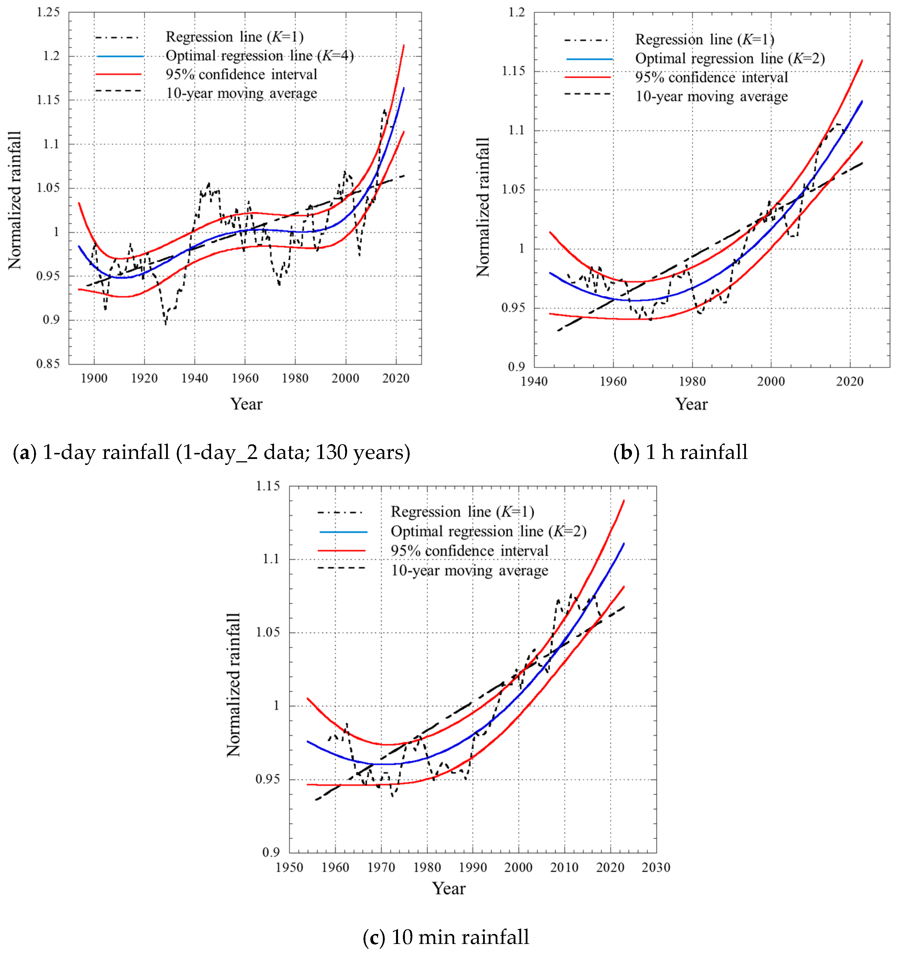
4.2. Polynomial Approximation

The polynomial approximation given by Equation (4) is applied. By adding one more parameter of σ² to K + 1 model parameters, the number of parameters N_p here is K + 2, and the AIC value can be calculated by Equation (7).

Table 3. Maximum log-likelihood and the AIC evaluation value of polynomial approximation. (The best K value is indicated in red).

Rainfall	K	${\widehat{\mathit{\sigma }}}^2$	$\mathit{l}({\hat{\mathit{\theta }}}^2)$	AIC	∆AIC
1-day	1	0.16089	−2956.79	5919.57	13.79
	2	0.16069	−2953.13	5914.26	8.472
	3	0.16059	−2951.24	5912.49	6.704
	4	0.16035	−2946.89	5905.78	0
	5	0.16033	−2946.60	5907.19	1.409
1-h	1	0.13068	−1445.22	2896.44	14.31
	2	0.13009	−1437.07	2882.13	0
	3	0.13009	−1437.02	2884.04	1.913
	4	0.13003	−1436.19	2884.37	2.241
	5	0.13002	−1436.10	2886.20	4.070
10-min	1	0.08708	−653.04	1312.07	13.57
	2	0.08667	−645.25	1298.51	0
	3	0.08662	−644.32	1298.65	0.137
	4	0.08660	−643.95	1299.90	1.392
	5	0.08657	−643.37	1300.73	2.222

shows the mean square residual (maximum likelihood estimate of variance ${\widehat{\sigma }}^2$), the log maximum likelihood (l($\widehat{\mathit{\theta }}$,${\widehat{\sigma }}^2$)), the AIC value (AIC), and the difference from the minimum value (AIC) for models K = 1 to 5. From the table, K = 4, 2, and 2 (shown in red) are the selected values that give the smallest AIC values for the 1-day, 1 h, and 10 min rainfalls, respectively. Thus, they are considered optimal among polynomial approximation models. Figure 5 shows the regression curves for the three rainfall types with the value of K selected according to the AIC, together with the linear regression line (K = 1). Lines showing 95% confidence intervals are also given in the figures. Since the calculation scheme of confidence interval in the case of non-linear regression lines is somewhat complicated, we used a Matlab software (R2022a) function “policonf”. For reference, the dotted line in the figure shows the 10-year moving average of the normalized rainfall values.

Although the optimal polynomial degree K is not the same for all three rainfall types, a common characteristic can be seen that a noticeable increasing trend begins around the year 1990. Looking at each optimal regression line after the year 1990, the trend shows more than a 10% increase up to now. The trend is also supported by the 95% confidence interval analysis as shown in the figure.

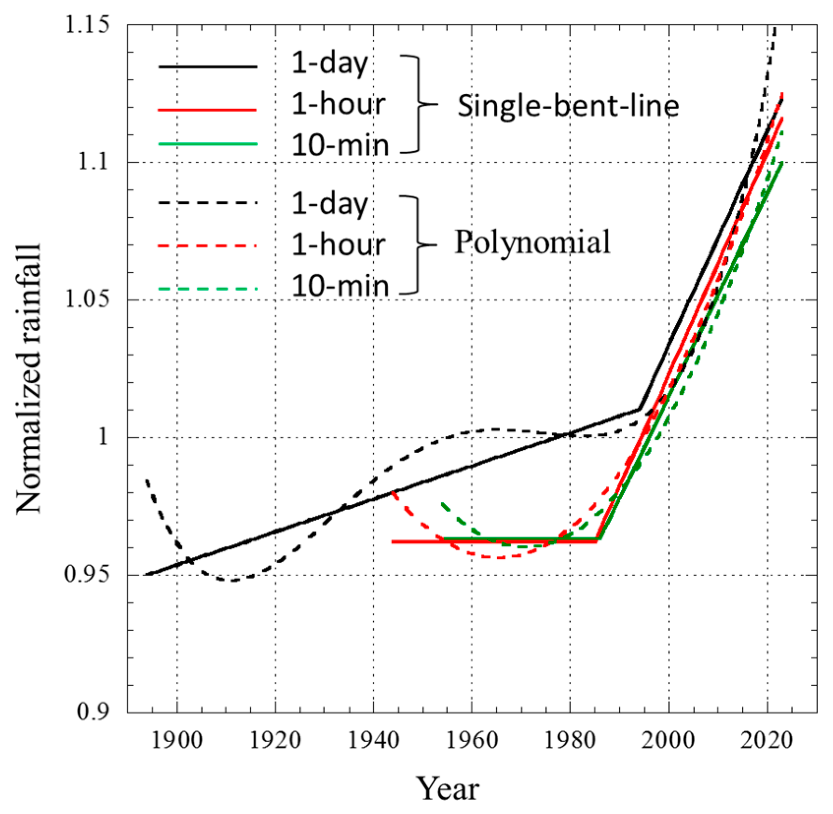
4.3. Single-Bent-Line Approximation

The polynomial approximation shown in the previous subsection for the annual maximum rainfall values made it appear that an increase had begun around 1990. Therefore, in order to clarify this turning point more clearly, we evaluate it using a single-bent-line approximation given in Equation (5). In addition to the model with four parameters (p = 4) of a, b, c, and d, the model with three parameters (p = 3) of b, c, and d after setting a = 0 is also evaluated. The steepest descent method was used to optimize the coefficients to obtain the maximum likelihood function. The evaluation formula for the AIC is used in (7) with N_p = p + 1.

Table 4. Evaluation of the long-term trends of three types of normalized maximum annual rainfalls using the AIC for single-bent-line approximations. (The best values are highlighted in red).

Rainfall	p	${\widehat{\mathit{\sigma }}}^2$	$\mathit{l}({\hat{\mathit{\theta }}}^2)$	AIC	∆AIC
1-day	3	0.16067	−2952.75	5913.50	7.72
	4	0.16052	−2949.95	5909.89	4.11
1-h	3	0.13003	−1436.13	2880.25	−1.88
	4	0.13002	−1436.05	2882.10	−0.03
10-min	3	0.08661	−644.10	1296.21	−2.30
	4	0.08659	−643.78	1297.56	−0.94

summarizes the evaluation results using AIC. The ΔAIC in the table shows the difference from the minimum AIC value (in red) for each rainfall in Table 3. From Table 4, although the single-bent-line approximation for 1-day rainfall (130 years) is less superior to the polynomial approximation with K = 4, for 1 h rainfall (80 years) and 10 min rainfall (70 years), the single-bent-line approximation with p = 3 is superior.

Figure 6 shows the long-term trend of rainfall based on the single-bent-line approximation with the best parameter values determined by the AIC. For reference, the results of the polynomial approximation are also given by dotted lines. It can be understood that the single-bent-line approximation is insufficient for the 1-day rainfall, which has a much longer period than the other two rainfall cases. In the 1-day rainfall case, it seems better to consider that there are multiple bending points during the period, as expected from the polynomial approximation with K = 4. For the 1 h rainfall and 10 min rainfall, the single-bent-line approximation has a better evaluation value than the polynomial approximation. As is clear from the figure, all three types of rainfall show a common trend of increase by about 10% over approximately 25 years since around 1990.

In summary, Figure 4 shows the linear approximation (regression line) of the polynomial approximation of Equation (4) with K = 1, i.e., y = a₀ + a₁x. If we select the optimal coefficients a₀ and a₁ that minimize the square error in the linear approximation, we obtain the straight line in Figure 4. From this, we can only say that there is a linear increase during the period. If we adopt a higher degree of K, we can see the variation during the period. The results obtained in this way are shown in Figure 5 (or the dotted line in Figure 6). When the AIC is used to determine which estimate is better, the results in Table 3 and Table 4 are obtained, and the polynomial approximation with K = 4 for the 1-day rainfall case, for example, is shown to be superior. The shape of the maximum likelihood estimation curve differs depending on the model selected, but the AIC determines which model is superior. In any case, the common feature is that rainfall intensity has increased by a little over 10% during the subject period.

4.4. Expected Future Trend of Extreme Rainfall

As shown in Figure 6, three types of the annual maximum rainfall have gradually increased by approximately 10% every 25 years since around 1990. There are several possible scenarios for predicting the future of this increasing trend, which can be expressed as follows.

(i)

A linear increase of about 10% every 25 years will continue for several decades. Taking the year 2000 as the base year (h_R = 1), it will be about h_R = 1.2 around 2050. Furthermore, it will be about h_R = 1.4 around 2100.

(ii)

The increasing trend will accelerate in the future.

(iii)

The increasing trend seen recently is part of a long steady state, and this increasing trend will eventually saturate.

From the trends in Figure 6, scenario (i) seems probable, but we cannot say for sure which scenario will actually occur until we see data further into the future. Also, we cannot say for sure whether this rainfall trend is limited to Japan or represents a global trend until we see data from around the world. Global warming, which is thought to be the cause of the rainfall increase, may change depending on future activities of humanity aiming for a sustainable society, and therefore the issue of rainfall is also highly uncertain depending on human activity. Regarding future climate change, it is important to continue collecting data as well as to investigate the causes and take countermeasures.

5. Consideration on Consistency with Other Measurement Results in Japan

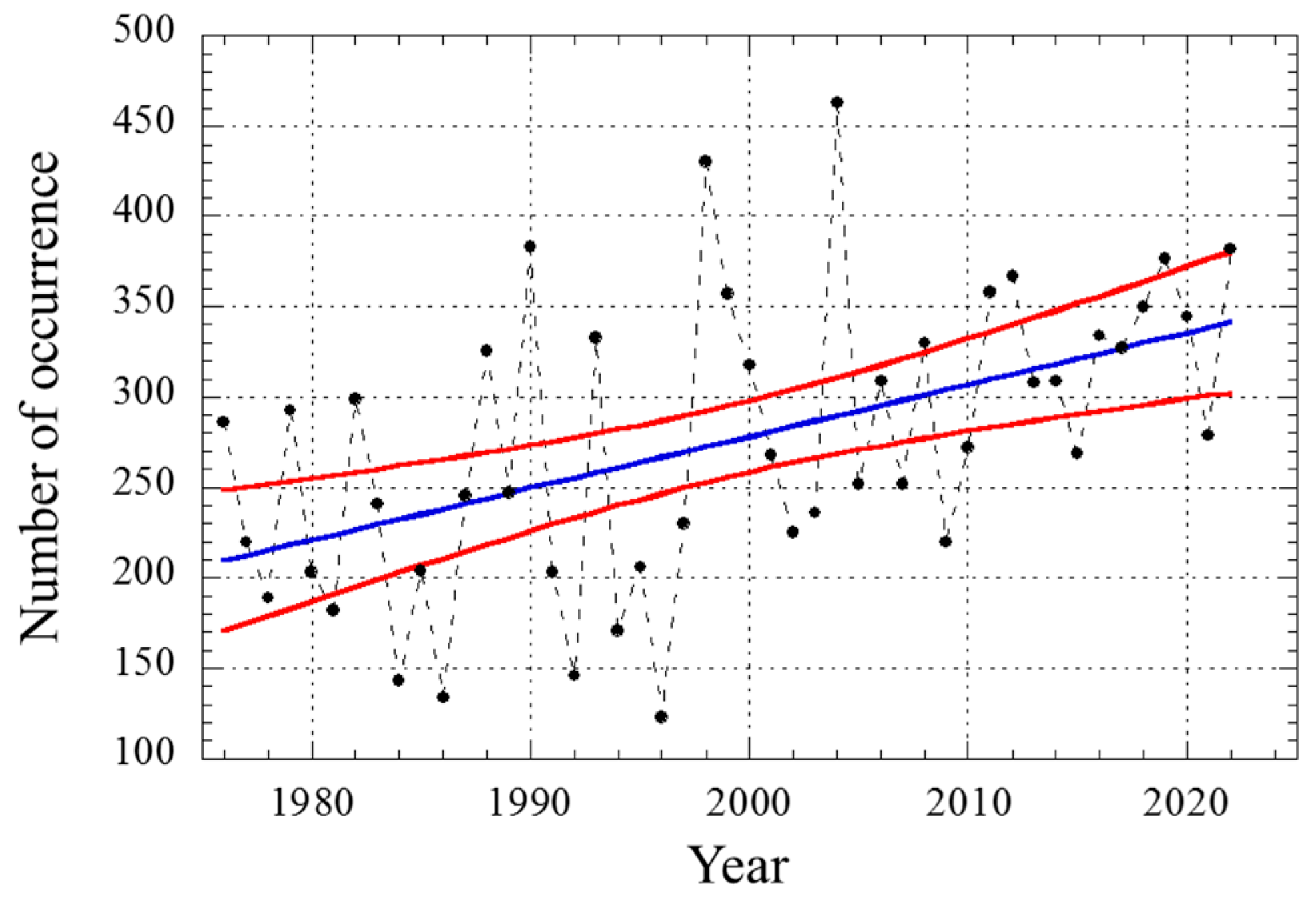
5.1. Increase in Heavy Rain Occurrence Frequency Evaluated by JMA

In the previous section, we analyzed the long-term trends of rainfall intensity, focusing on the annual maximum values of various rainfall types and found an increasing trend from around 1990. An analysis by the Japan Meteorological Agency (JMA) evaluated the number of event occurrences in which 1 h rainfall exceeded threshold values such as 50 mm, 80 mm, and 100 mm over the period from 1976 to 2022, using the AMeDAS data collected at approximately 1300 locations [21]. Figure 7 shows the results for the heavy rainfall case, in which rainfall exceeds a threshold of 50 mm per hour. The figure clearly indicates an increasing trend. According to the JMA report, the number of times that 1 h rainfall exceeded the 50 mm threshold during the most recent 10-year observation period (2013–2022) is 1.5 times the number of such cases in the first 10-year period (1976–1985) (328 times/226 times). For the 80 mm threshold, the ratio is 1.8 (25/14), and for the 100 mm threshold, the ratio is 2.0 (4.4/2.2). Based on these results, the JMA concluded that the occurrence of heavy rain events has gradually increased in recent years.

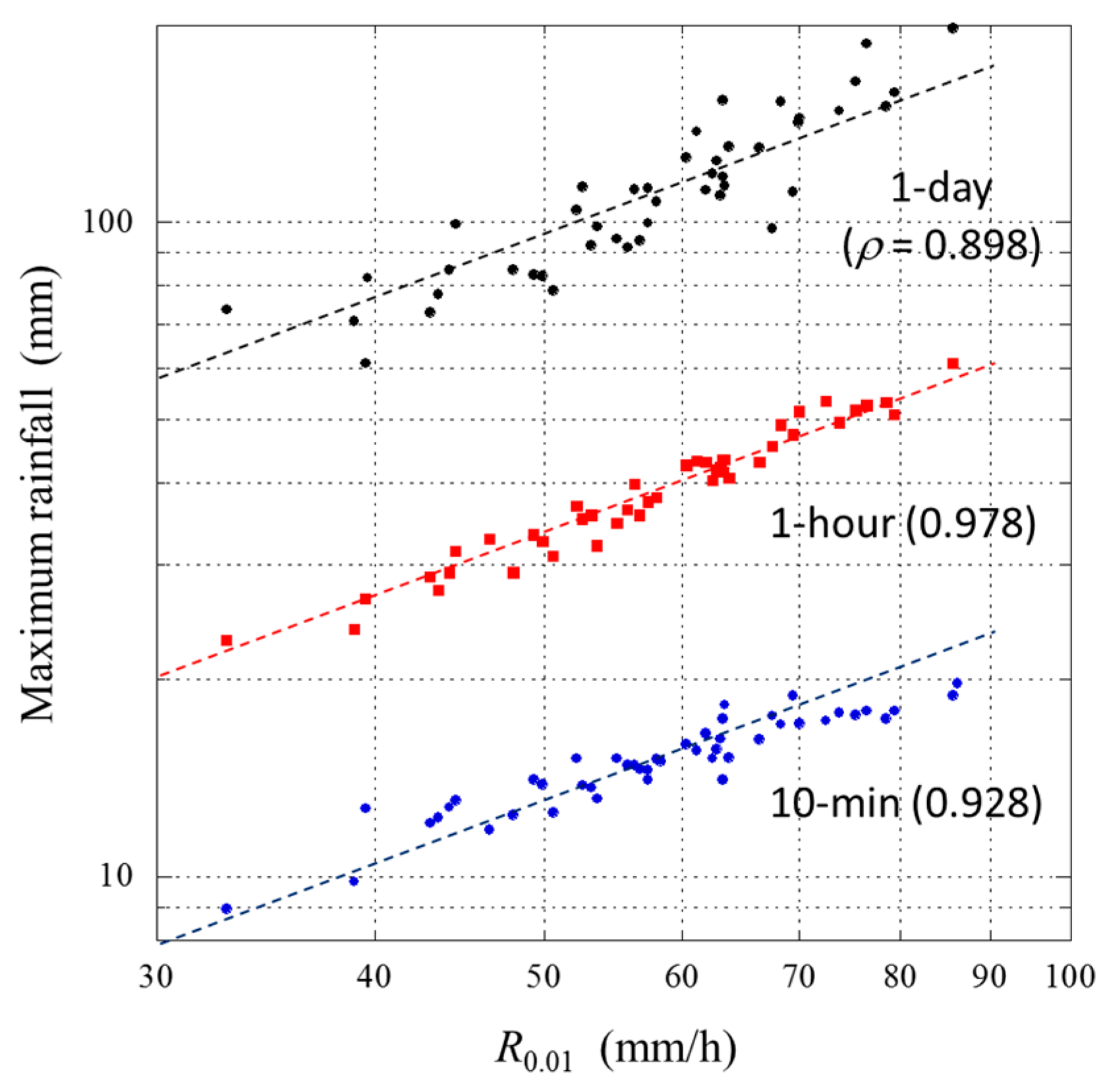
5.2. Heavy Rain Occurrence Increase Ratio vs. Rainfall Intensity Increase Ratio

In Section 4, we described the long-term changes in the annual maximum 1-day, 1 h, and 10 min rainfalls. Viewed from the perspective of a cumulative probability distribution of rainfall intensity averaged over a long period, the annual maximum values correspond to time percentages of 0.274% (=1/365) for 1-day rainfall, 0.0114% (=1/(365 × 24)) for 1 h rainfall, and 0.0019% (=1/(365 × 24 × 6)) for 10 min rainfall. Below, we focus on the probability distribution of 1 h rainfall to examine the compatibility of the JMA report with our results.

It has been found that the probability distribution of rainfall in Japan can be well approximated by Hosoya’s M distribution, shown below, for both 1 min rainfall rate and 1 h rainfall amount [22].

$$\mathrm{PDF:\hspace{1em}}f(R)={\displaystyle \frac{\alpha }{R}}\left({\displaystyle \frac{1}{R}}+\beta \right)e^{-\beta R}$$

(8a)

$$\mathrm{CDF:\hspace{1em}}F(R)={\displaystyle {\int }_R^{\infty }f(R)dR=}{\displaystyle \frac{\alpha }{R}}{e}^{-\beta R} (R\ge R_{\min }\mathrm{ where }F\left(R_{\min }\right)=1)$$

(8b)

where α and β are parameters that depend on the rainfall type and location. The distribution of rainfall intensity fits well to a gamma distribution for the lower cumulative probability part (i.e., heavy rain part) and to a log-normal distribution for the higher cumulative probability part (i.e., light rain part). As an example of the cumulative 1 h rainfall distribution, the case of Kumamoto (site number 42 in Table 1) which is located in top 10 percent of heavy-rain areas in Japan, is shown in Figure 8 by the dotted line for the 30 years from 1951 to 1980. The black solid line labeled F₀ in the figure, with α = 0.0888 ≡ α₀ and β = 0.07151 ≡ β₀, gives the distribution in (8b).

From the maximum likelihood estimation analysis shown in Figure 6, it can be seen that there has been an increase in more than 10% from the earlier period before the increasing trend began. Let the cumulative probability after the increase be F₁, with α₁ and β₁; then, the cumulative distribution of rainfall R, when assuming an increase by a constant ratio η_R, is given by the following equation:

$$F_1(R)=F_0\left({\displaystyle \frac{R}{{\eta }_R}}\right)={\displaystyle \frac{{\alpha }_1}{R}}{e}^{-{\beta }_{1}R},\hspace{1em}{\alpha }_1={\eta }_R{\alpha }_0,\hspace{1em}{\beta }_1={\displaystyle \frac{1}{{\eta }_R}}{\beta }_0$$

(9)

Call η_R the rainfall intensity increase ratio. The red line F₁ in Figure 8 shows the calculated CDF for 1 h rainfall multiplied by η_R = 1.1 for each rainfall value of F₀, shown as an example. The upward movement of the curve in this way is useful for understanding the increase in the intensity of rainfall seen at a specific point of cumulative time percentage of p₀. In this case, the average annual maximum 1 h rainfall corresponds to the value for approximately 0.011% of the time.

On the other hand, the F₁ curve can be seen as having moved to the right from the F₀ curve, and its occurrence increase ratio η_p depends on the cumulative time percentage p. The ratio η_p is the increase ratio of the time percentage when rainfall exceeds the threshold value R. Since the rainfall is measured every hour, the increase ratio η_p can be interpreted as the rate of increase in the number of occurrences of events where the 1 h rainfall exceeds the given threshold. From the JMA data shown in Figure 6, we can identify the value of η_p.

Consider the ratio η_p = F₁/F₀, the rate of increase in the number of occurrences, as a function of rainfall R. The ratio can be expressed as follows:

$${\eta }_p\left(\equiv {\displaystyle \frac{F_1(R)}{F_0(R)}}\right)={\eta }_R\exp \left\{-\left({\displaystyle \frac{1}{{\eta }_R}}-1\right){\beta }_{0}R\right\}$$

(10)

Figure 9 shows the occurrence increase ratio η_p (=F₁/F₀) as a function of 1 h rainfall, with the rainfall intensity increase ratio η_R as a parameter. The parameter values of α and β for the reference cumulative distribution F₀ are those from Kumamoto data in Figure 8. The figure also plots the results shown in the JMA report. In the JMA report, the increase in frequency of occurrence is given as the ratio of the average value of the last 10 years (2013–2022) to the first 10 years (1976–1985). Looking at the rainfall increase ratio η_R of 1 h rainfall in Figure 6 for the middle years of each period, 1980 and 2017, it is about 1.1, and the data from Kumamoto matches this very well. Although the JMA results use data from all of Japan without normalization, it seems reasonable to consider that the dominant contribution is mainly due to heavy rain areas such as Kumamoto.

As a matter of course, it cannot be directly compared to the data from Kumamoto alone. For the seven locations in the Kyushu region (Sites No. 39–45), which belong to a heavy-rain area in Japan, the cumulative distribution of 1 h rainfall over five years (1956–1960) was calculated, and the fitted parameter values of a = 0.0661 and b = 0.0716 were obtained. As shown in Equation (10), h_p in Figure 9 depends only on the parameter value of b, and this value is almost the same as in the Kumamoto case (b = 0.0715). As a result, the calculation results shown in Figure 9 are commonly valid in heavy-rain areas in Japan.

6. Impact on Rain Attenuation Estimation Models

As mentioned at the beginning of the introduction of this paper, in wireless communication using radio waves with frequencies above 10 GHz, attenuation due to rain causes a serious problem in link design. For this reason, a rain attenuation estimation method using rainfall intensity data for the relevant area has been developed. For Earth–space and terrestrial radio links, the calculation formula for rain attenuation recommended by the ITU-R [1,2] is as follows:

$$A_{0.01}=a{R}_{0.01}^b{L}_e$$

(11)

where A_0.01 is the rain attenuation in decibels, corresponding to a cumulative probability of 0.01% in an average year; L_e is the effective path length of the corresponding rain area; and a and b are the frequency-dependent coefficients given in [23]. Rain attenuation for p% of the time A_p can be calculated using A_0.01. R_0.01, in mm/h, is the rainfall rate that is exceeded during 0.01% of the cumulative time in an average year. The site-by-site rainfall rate data were obtained on a 1 min integration basis and is referred to as the 1 min rainfall rate. The development of Equation (11) by the ITU-R has a long history, beginning in the 1980s, where it was used to test the performance of calculation methods available to that point, as summarized in [24], and such improving effort has continued until now. Taking the shower-like heavy-rain frequently encountered in Asian tropical areas into account, the ITU-R provides a calculation scheme with sufficiently high accuracy and keeps the basic formula in (11) while extending it for global use [1].

Table 1 also shows the 1 min rainfall rate for 0.01% of the time, R_0.01, used in Japan [4]. The values were derived by using the cumulative time distribution (CDF) of various types of rainfall, with different integration times measured by the automated meteorological data acquisition system, AMeDAS, at 1300 sites throughout Japan. The AMeDAS has collected 1 h rainfall data since 1976, 10 min rainfall data since 1995, and 1 min rainfall data since 1996. The calculation of R_0.01 uses the data from 1977 to 2002, covering approximately 26 years. Priority is given to using rainfall types with shorter integration times, and a method for converting to R_0.01 from the various types of rainfall was developed [5,25]. At present, the obtained values are considered the most reliable estimates of R_0.01. As a result, the Japanese Ministry of Internal Affairs and Communications, MIC, recommends their use in designing radio systems in Japan [4].

The scatterplots in Figure 10 show the relationship between R_0.01 and the annual maximum 1-day (1-day_1 data), 1 h, and 10 min rainfall amounts listed in Table 1. From the figure, there appears to be a strong linear relationship in all three cases, with correlation coefficients of 0.898, 0.978, and 0.928 for the 1-day, 1 h, and 10 min rainfalls, respectively. The correlation for 1 h rainfall (0.978) is particularly high. In terms of integration time, the correlation of the 1 min rainfall rate R_0.01 with the 10 min rainfall rate is considered higher; however, the saturation effect observed in areas where R_0.01 > 70 mm reduces the correlation value. Accordingly, we can expect that the long-term trend of R_0.01 closely follows that of the average annual maximum 1 h rainfall.

The reason for seeing the saturation effect in the case of the 10-minute rainfall is due to the difference in the cumulative time percentage that is being focused on. The 1 min rainfall intensity of R_0.01 corresponds to 0.01% of time, namely, the worst 53 min in a year. On the other hand, the annual maximum value of 10 min rainfall corresponds to a time rate of 0.002%, namely, the worst 10 min in a year. In general, saturation phenomena tend to appear in areas with small time percentages; therefore, the annual maximum value of 10 min rainfall is likely to show a saturation effect compared with 1 h and 1-day rainfalls.

It would be desirable to investigate the long-term change characteristics of the measured R_0.01 data themselves, but there were not enough data to verify the trend, so we investigated the correlation with the average annual maximum rainfall value at each point. On the other hand, a good linear relationship between R_0.01 values measured in 48 locations in Japan derived from cumulative distribution characteristics during each period and the average annual maximum 1 h rainfall values there has been identified in [26].

Considering that the average value of the annual maximum 1 h rainfall at each location in Japan is proportional to R_0.01 with a very high correlation, it is expected that the rainfall increase coefficient η_R in the long-term change characteristics of the annual maximum 1 h rainfall discussed in Section 4.4 also represents the long-term change characteristics of R_0.01 in the near future.

It should be noted that, because the basic rainfall data were collected in Japan, the predicted value of η_R is also applicable only to Japan. The long-term variation characteristics of rainfall are expected to be highly region-dependent, and therefore long-term change prediction for the ITU-R database [3] will require a similar evaluation using long-term rainfall data on a global scale. Accordingly, future research efforts should include the following:

(1)

Rainfall increasing ratio h_R should be reviewed in 2050 or so using the 1 h rainfall data available for Japan at that time in order to determine whether the projected trend remains unchanged or not.

(2)

Future trend projections should be extended to a global scale. As described, rainfall characteristics differ depending on the regional climate. Consequently, annual change trends will also differ. As discussed in [19], it is difficult to draw a conclusion for a specific location even when rainfall data are collected at that location over a period as long as 100 years. Thus, grouping together multiple sites located in similar climate zones and looking for common trends from the large amount of rainfall data that result would seem to offer an effective analytical approach. In such a case, it would be realistic to identify the change trend from the characteristics of the annual maximum 1 h rainfall following the method mentioned in this paper.

(3)

As shown in Equation (11), in addition to R_0.01, to know the long-term change in the equivalent path length L_e is also important for estimating rain attenuation. Because evaluating the equivalent path length involves using the trend in the spatial spread of the rain area, the estimation is more difficult than in the case of predicting the change in R_0.01 from site-specific rainfall data. Accordingly, to develop a reliable rain attenuation prediction scheme in the future, research not only on R_0.01 but also on L_e will be essential.

7. Conclusions

This study used extreme rainfall data (annual maximum rainfall) in Japan to identify long-term trends in rainfall statistics. The goal was to determine whether R_0.01, a value used to estimate rain attenuation when designing wireless communication systems, is changing, possibly due to the effects of global warming. Noting that the R_0.01 values in Japan, which can be found in a publicly available database, are linearly related to long-term average annual maximum 1 h rainfall and that the two sets of values have an extremely high correlation, we investigated the long-term trends for three types of rainfall, including 1 h rainfall. Our findings can be summarized as follows:

(1)

Because rainfall varies widely from year to year, a noticeable long-term trend could not be confirmed using site-by-site data and a 95% confidence interval analysis, even with 100 years of data.

(2)

By dividing the annual maximum rainfall by the long-term average rainfall site-by-site and using these normalized values in the analysis, an increasing trend of more than 10% was identified [19].

(3)

By applying non-linear function approximations whose optimal order is determined based on the AIC, the increasing trend became more noticeable from the 1990s onward.

Regarding R_0.01, the 1 min rainfall rate used in rain attenuation prediction models:

(4)

A linear relationship was found between R_0.01 and the long-term average of the annual maximum rainfall values for the three types of rainfall (1-day, 1 h and 10 min). An especially high correlation (0.978) was observed for the 1 h rainfall case.

(5)

Considering the above, we can expect that the long-term variation of R_0.01 will follow the same trend as that of 1 h rainfall. If this is the case, then the R_0.01 database should be revised in the near future, taking the increasing ratio h_R into account.

The long-term changes in rainfall described in this paper are thought to include the effects of global warming; however, to clarify this point, a similar analysis on a global scale with diverse climate characteristics will be necessary. It should be further noted that the long-term changes in R_0.01 predicted by the formula developed in this study applied only to Japan. Predictions on a global scale have yet to be made, and it is hoped that the evaluation method featured here will be of significant value in facilitating such predictions.

Moreover, for establishing a revised calculation scheme for rain attenuation based on Equation (11) in the future, it becomes necessary to evaluate the trend of not only R_0.01 but also the effective path length. Since the effective path length depends on the horizontal spreading of the rain area and the rain height (height of the 0 °C layer), it seems more difficult than R_0.01, which is determined only by the point rainfall amount. This should also be raised as a future research topic.

In this paper, we used measured rainfall data published by the Japan Meteorological Agency to clarify the statistical characteristics of the long-term variations in rainfall in Japan. In addition to this kind of statistical approach, it is also important to make clear the physics of long-term changes in rainfall. To achieve this, academic research based on meteorological science is required. We look forward to the progress of research in this field.

References

1. ITU-R. Propagation Data and Prediction Methods Required for the Design of Earth-Space Telecommunication Systems; Document ITU-R, ITU-R Rec. P.618-14; ITU-R: Geneva, Switzerland, 2023. [Google Scholar]
2. ITU-R. Propagation Data and Prediction Methods Required for the Design of Terrestrial Line-of-Sight Systems; Document ITU-R, ITU-R Rec. P.530-18; ITU-R: Geneva, Switzerland, 2021. [Google Scholar]
3. ITU-R. Characteristics of Precipitation for Propagation Modelling; Document ITU-R, ITU-R Rec. P.837-7; ITU-R: Geneva, Switzerland, 2017. [Google Scholar]
4. MIC. Radio Regulation-Related Inspection Standard for Fixed Radio Station (In Japanese); The Ministry of Internal Affairs and Communications (MIC): Tokyo, Japan, 2011. [Google Scholar]
5. Ono, K.; Karasawa, Y. M-distribution-based rain attenuation distribution prediction method introducing safety factor. IEICE Trans. Commun. 2008, J91-B, 169–187. (In Japanese) [Google Scholar]
6. IPCC. Climatic Change 2013: The Physical Science Basis; IPCC: Geneva, Switzerland, 2013. [Google Scholar]
7. JMA. Global Warming Prediction Information (In Japanese); Japan Meteorological Agency: Tokyo, Japan, 2017; Volume 9, Available online: https://www.data.jma.go.jp/cpdinfo/GWP/Vol9/pdf/all.pdf (accessed on 4 July 2025).
8. JMA. Japan’s Climate Change 2020 (In Japanese); Japan Meteorological Agency: Tokyo, Japan, 2020; Available online: https://www.data.jma.go.jp/cpdinfo/ccj/index.html (accessed on 4 July 2025).
9. Trenberth, K.E. Changes in precipitation with climate change. Clim. Res. 2011, 47, 123–138. [Google Scholar] [CrossRef]
10. Adler, R.F.; Sapiano, M.R.P.; Huffman, G.J.; Wang, J.-J.; Gu, G.; Bolvin, D.; Chiu, L.; Schneider, U.; Becker, A.; Nelkin, E.; et al. The global precipitation climatology project (GPCP) monthly analysis (new version 2.3) and a review of 2017 global precipitation. Atmosphere 2018, 9, 138. [Google Scholar] [CrossRef] [PubMed]
11. Donat, M.G.; Lowry, A.L.; Alexander, L.V.; O’Gorman, P.A.; Maher, N. More extreme precipitation in the world’s dry and wet regions. Nat. Clim. Chang. 2016, 6, 508–513. [Google Scholar] [CrossRef]
12. Shiogama, H.; Imada, Y.; Mori, M.; Mizuta, R.; Stone, D.; Yoshida, K.; Arakawa, O.; Ikeda, M.; Takahashi, C.; Arai, M.; et al. Attributing historical changes in probabilities of record-breaking daily temperature and precipitations extreme events. SOLA 2016, 12, 225–231. [Google Scholar] [CrossRef]
13. Allan, R.P.; Soden, B.J.; O John, V.; Ingram, W.; Good, P. Current changes in tropical precipitation. Environ. Res. Lett. 2010, 5, 025205. [Google Scholar] [CrossRef]
14. Groisman, P.Y.; Knight, R.W.; Easterling, D.R.; Karl, T.R.; Hegerl, G.C.; Razuvaev, V.N. Trends in intense precipitation in the climate record. J. Clim. 2005, 18, 1326–1350. [Google Scholar] [CrossRef]
15. Lenderink, G.; Mok, H.Y.; Lee, T.C.; van Oldenborgh, G.J. Scaling and trends of hourly precipitation extremes in two different climate zones—Hong Kong and the Netherlands. Hydrol. Earth Syst. Sci. 2011, 15, 3033–3041. [Google Scholar] [CrossRef]
16. Zhou, Y.; Lau, W.K. The relationships between the trends of mean and extreme precipitation. Int. J. Clim. 2017, 37, 3883–3894. [Google Scholar] [CrossRef]
17. Demirdjian, L.; Zhou, Y.; Huffman, G.J. Statistical modeling of extreme precipitation with TRMM data. J. Appl. Meteorol. Clim. 2018, 57, 15–30. [Google Scholar] [CrossRef] [PubMed]
18. JMA. Past Weather Data Search (in Japanese). Japan Meteorological Agency Open Website. Available online: https://www.data.jma.go.jp/obd/stats/etrn/index.php (accessed on 4 July 2025).
19. Karasawa, Y. Long-term statistical properties of extreme rainfall data in Japan. IEEE Trans. Geosci. Remote Sens. 2024, 62, 4707912. [Google Scholar] [CrossRef]
20. Akaike, H. A new look at the statistical model identification. IEEE Trans. Autom. Control 1974, 19, 716–723. [Google Scholar] [CrossRef]
21. JMA. Past Changes in Heavy Rain and Extremely Hot Days (Extreme Phenomena), (In Japanese); Japan Meteorological Agency: Tokyo, Japan, 2025; Available online: https://www.data.jma.go.jp/cpdinfo/extreme/extreme_p.html (accessed on 4 July 2025).
22. Hosoya, Y. An estimation method for one-minute rain distributions at various locations in Japan. IEICE Trans. Commun. 1988, J71-B, 256–262. (In Japanese) [Google Scholar]
23. ITU-R. Specific Attenuation Model for Rain for Use in Prediction Methods; Document ITU-R, ITU-R Rec. P.838-3; ITU-R: Geneva, Switzerland, 2005. [Google Scholar]
24. Yamada, M.; Karasawa, Y.; Yasunaga, M.; Arbesser-Rastburg, B. An improved prediction method for rain attenuation in satellite communications operating at 10–20 GHz. Radio Sci. 1987, 22, 1053–1062. [Google Scholar] [CrossRef]
25. Ono, K.; Karasawa, Y. An accurate conversion method of different integration rate CDF using M-distribution applicable to all over Japan. IEICE Trans. Commun. 2007, J90-B, 266–279. (In Japanese) [Google Scholar]
26. Karasawa, Y.; Matsudo, T. One-minute rain rate distributions in Japan derived from AMeDAS one-hour rain rate data. IEEE Trans. Geosci. Remote Sens. 1991, 29, 890–898. [Google Scholar] [CrossRef]
Figure 1. Observation sites and the average of annual maximum 1 h rainfall. (In Table 1, values are not included for Nara (site 46) and Naha (site 47), because the observation period was short, but the map gives the average value for the observation period (1954–2023)).
Climate 13 00145 g001
Figure 2. Mean value of annual maximum 1-day rainfall (data: 1-day_1) and the standard deviation of normalized 1-day rainfall at various sites in Japan.
Climate 13 00145 g002
Figure 3. Long-term trend of annual maximum 1 h rainfall in Tokyo (Site 13). (The central blue line is the regression line; the upper and lower red curves are the 95% confidence interval boundaries).
Climate 13 00145 g003
Figure 4. Long-term trend of the normalized 1 h rainfall for all of Japan. (The central blue line is the regression line; the upper and lower red curves are the 95% confidence interval boundaries).
Climate 13 00145 g004
Figure 5. Polynomial approximation of year-to-year variation for three types of normalized rainfall. In each case, the polynomial was selected using the AIC.
Climate 13 00145 g005
Figure 6. Long-term change characteristics of three types of precipitation (dotted line: polynomial approximation, solid line: simple broken line approximation).
Climate 13 00145 g006
Figure 7. Number of annual occurrences of heavy rain with 1 h rainfall of more than 50 mm at approximately 1300 locations across Japan (numerical data are from [21]). (Blue line is the regression line; red lines are the 95% confidence interval boundaries).
Climate 13 00145 g007
Figure 8. CDF of measured 1 h rainfall in Kumamoto (site No. 42) for 30 years, from 1951 to 1980, and its approximation by (8b) noted by F0 with the expected CDF at present (F1). Note: From Table 1, the average value of the annual maximum 1 h rainfall in Kumamoto (site No. 42) is 51.61 mm. On the other hand, the 0.01% value, which corresponds roughly to the annual maximum 1 h rainfall, has a value of approximately 42 mm for F0. This discrepancy is due to the difference in the definition of the maximum 1 h rainfall. The 1 h rainfall used in the cumulative distribution in Figure 8 is measured every hour, such as at 1 a.m., 2 a.m., and so on, while the annual maximum 1 h rainfall reported by the JMA, which we used in our analysis, is the true maximum value for one hour starting at any time in the year. As a result, the annual maximum 1 h rainfall reported by the JMA is almost always larger than the annual maximum 1 h rainfall used in the CDF analysis, as is shown in Figure 8.
Climate 13 00145 g008
Figure 9. Increase ratio of events where 1 h rainfall exceeds threshold R for the CDF of F0 shown in Figure 8. The result from the AMeDAS observation reported by the JMA [21] is also plotted by dots as reference purposes.
Climate 13 00145 g009
Figure 10. Scatter plot showing the relationship between R0.01 and the average value of 1-day (1-day_1), 1 h, and 10 min rainfall given in Table 1. Each straight line represents the linear relation between the two.
Climate 13 00145 g010